Modeling Healthcare Data with a Novel Flexible Three-Parameter Distribution

Abstract
1. Introduction
2. Exponentiated STH-II Distribution
- When , the ESTH-II distribution reduces to the STH-II distribution with parameters and .
- Setting , the ESTH-II yields the ESTH-I model, representing a new model.
Asymptotic Behavior
- If then .
- If then .
- If then .
3. Statistical Properties
3.1. Quantiles and Random Samples’ Generation
| Algorithm 1 Quantile computation for ESTH-II |
| Input: Parameters , , ; quantile level |
|
3.2. Random Sample Generation
| Algorithm 2 Random number generation from |
| Input: Parameters , , ; sample size |
|
3.3. Effect of Model Parameters on Quartiles
- 1.
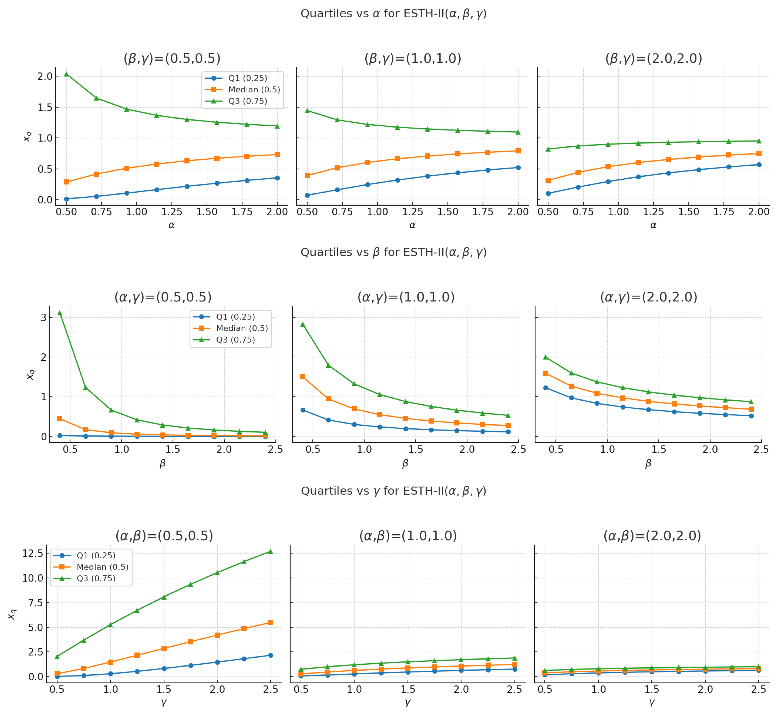
- Quartiles as a Function of : When and are held constant, increasing generally raises the lower quartile and the median. For small and , the upper quartile decreases as increases, indicating a tighter distribution with a reduced upper tail. This effect is strongest when both and are small. For larger values of and , the upper quartile remains nearly constant, and the three quartiles converge, yielding a more symmetric, compact distribution.
- 2.
- Quartiles as a Function of : As increases, all three quartiles decrease, regardless of the fixed values of and . The decline is steeper when and are small, and more gradual when they are large. As grows, the gap between quartiles narrows, reducing spread and skewness, and pushing the distribution toward symmetry.
- 3.
- Quartiles as a Function of : When and are small, increasing raises all quartiles, especially the upper one, indicating a heavier right tail and greater spread. For larger and , the influence of diminishes, and the distribution remains narrower and more symmetric.
3.4. Moments
- Term 1: For ,
- Term 2: For ,
3.5. Moment-Generating Function
3.6. Skewness and Kurtosis
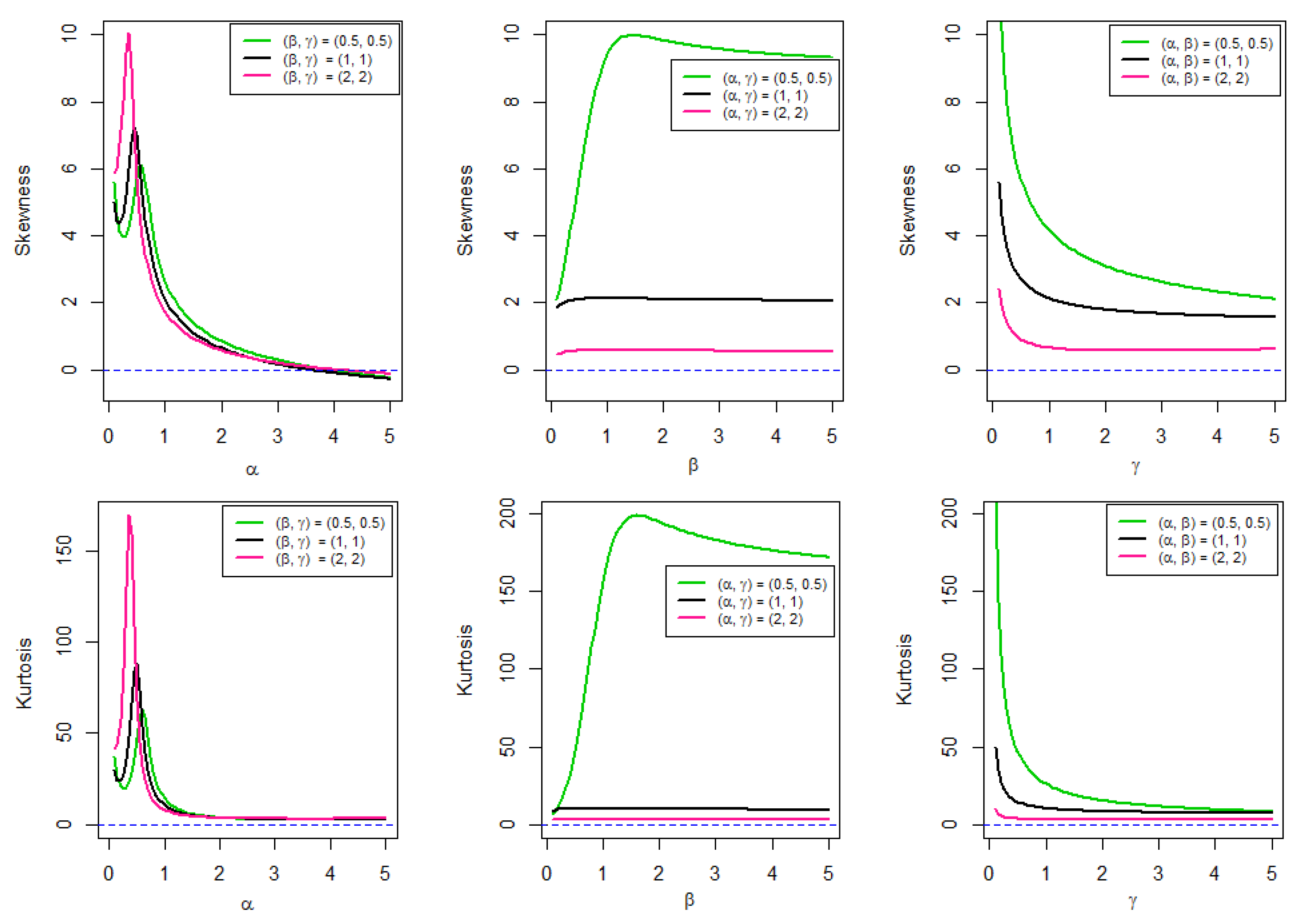
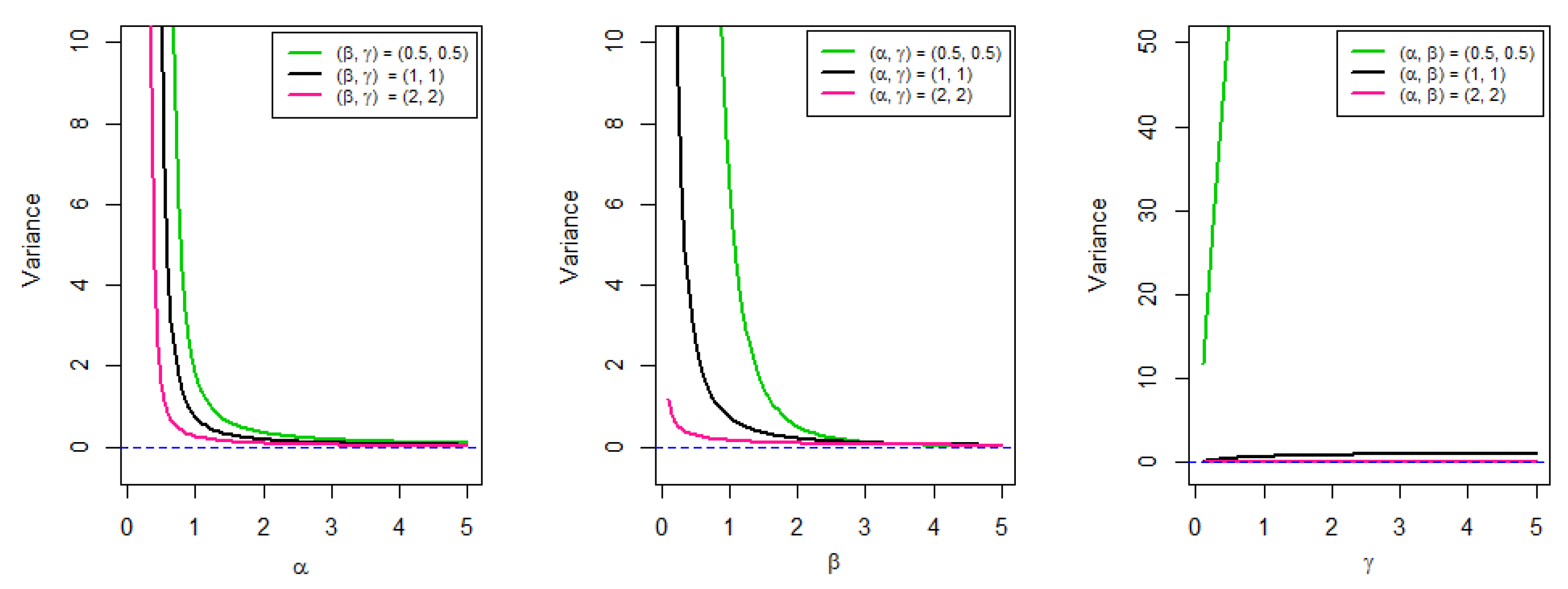
- Effect of : When and are held fixed, tends to elevate the central tendency of the ESTH-II distribution while simultaneously decreasing both skewness and kurtosis. This reflects a movement toward a more symmetric distribution with less influence from extreme values. The effect is particularly noticeable when and are small, whereas at higher values, the distribution curves begin to flatten. In essence, larger produces distributions that are more balanced, with lighter tails and reduced variability.
- Effect of : Holding and constant, variations in primarily affect the tail structure and concentration of the distribution. Increasing raises the mean and higher-order moments, shifting the mass toward larger values. The skewness and kurtosis are initially high for small , but stabilize as grows. Variance, however, decreases steadily with increasing . The sensitivity to is strongest when both and are small, while for larger values, the curves flatten and their influence diminishes.
- Effect of : With fixed, increasing produces systematic changes in the moments. For small , the distribution is highly skewed and heavy-tailed, especially when are small (e.g., 0.5). As increases, both the mean and variance rise steadily, while the skewness and kurtosis decrease, reflecting a move toward symmetry and lighter tails. This effect is more pronounced when are low, whereas for higher values (e.g., 2), the distribution stabilizes quickly and changes occur at a slower rate. Overall, acts as a scale and tail control factor, strongly influencing the distribution’s shape.
4. Parameter Estimation
4.1. Maximum Likelihood Estimation
Confidence Intervals
- 1.
- Calculate the standard errors ,
- 2.
- Determine the critical value from the standard normal distribution.
- 3.
- Construct the confidence intervals as follows:
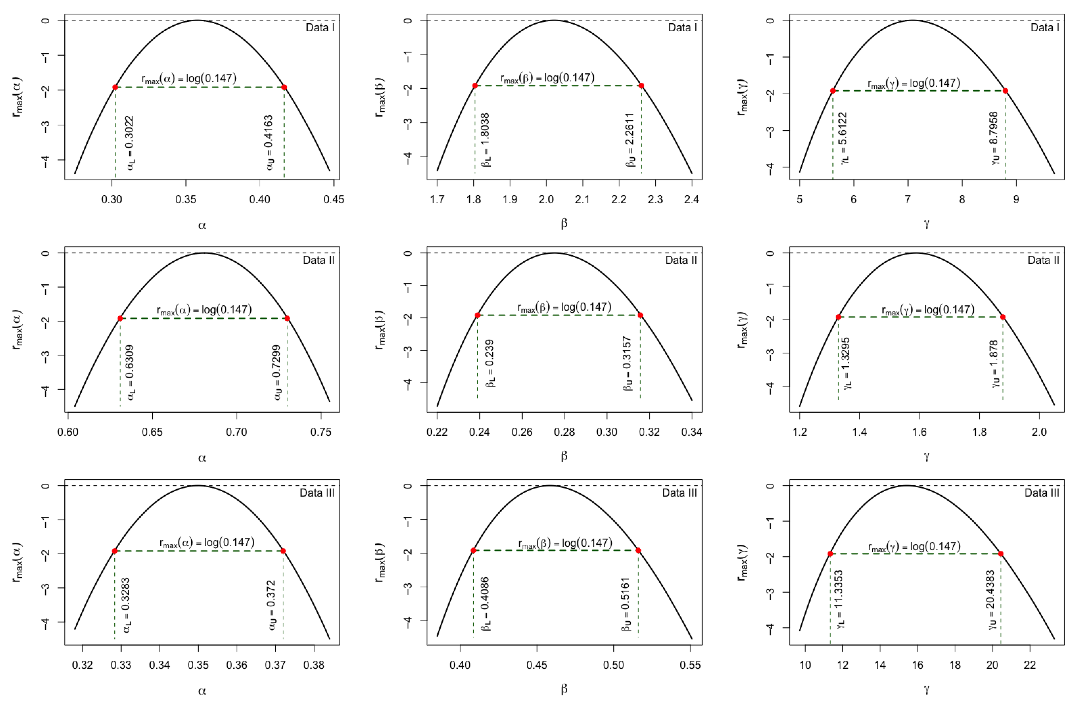
4.2. Likelihood Intervals
4.3. Bayesian Inference via Markov Chain Monte Carlo (MCMC)
- Model and priors.
- (i)
- Under the quadratic loss function (QLF), the Bayes estimator is the posterior mean, and the corresponding Bayes risk is the posterior variance.
- (ii)
- Under the absolute error loss function (ALF), the Bayes estimator is the posterior median, and the corresponding Bayes risk is the posterior expected absolute deviation from the posterior median.
- (iii)
- A credible interval for is obtained from the and quantiles of its marginal posterior distribution.
| Algorithm 3 Metropolis-within-Gibbs sampler for the ESTH-II posterior |
| Input: Data ; prior hyperparameters , , and ; iterations N; burn-in B; and proposal kernels , , |
| Output: Posterior draws |
|
5. Simulation Study
- (1)
- To examine the accuracy of maximum likelihood (MLE) and Bayesian estimators (under quadratic and absolute loss functions) in terms of average point estimates (APE) and mean squared error (MSE);
- (2)
- To evaluate the reliability of their interval estimates through coverage probabilities (CP);
- (3)
- To investigate how sample size influences the overall quality of parameter estimation.
5.1. Simulation Design and Algorithm
| Algorithm 4 Monte Carlo Simulation Procedure |
| Input: True parameter vectors ; sample sizes ; and number of replicates . |
| Output: Arrays of estimates , MSE values, and coverage indicators. |
|
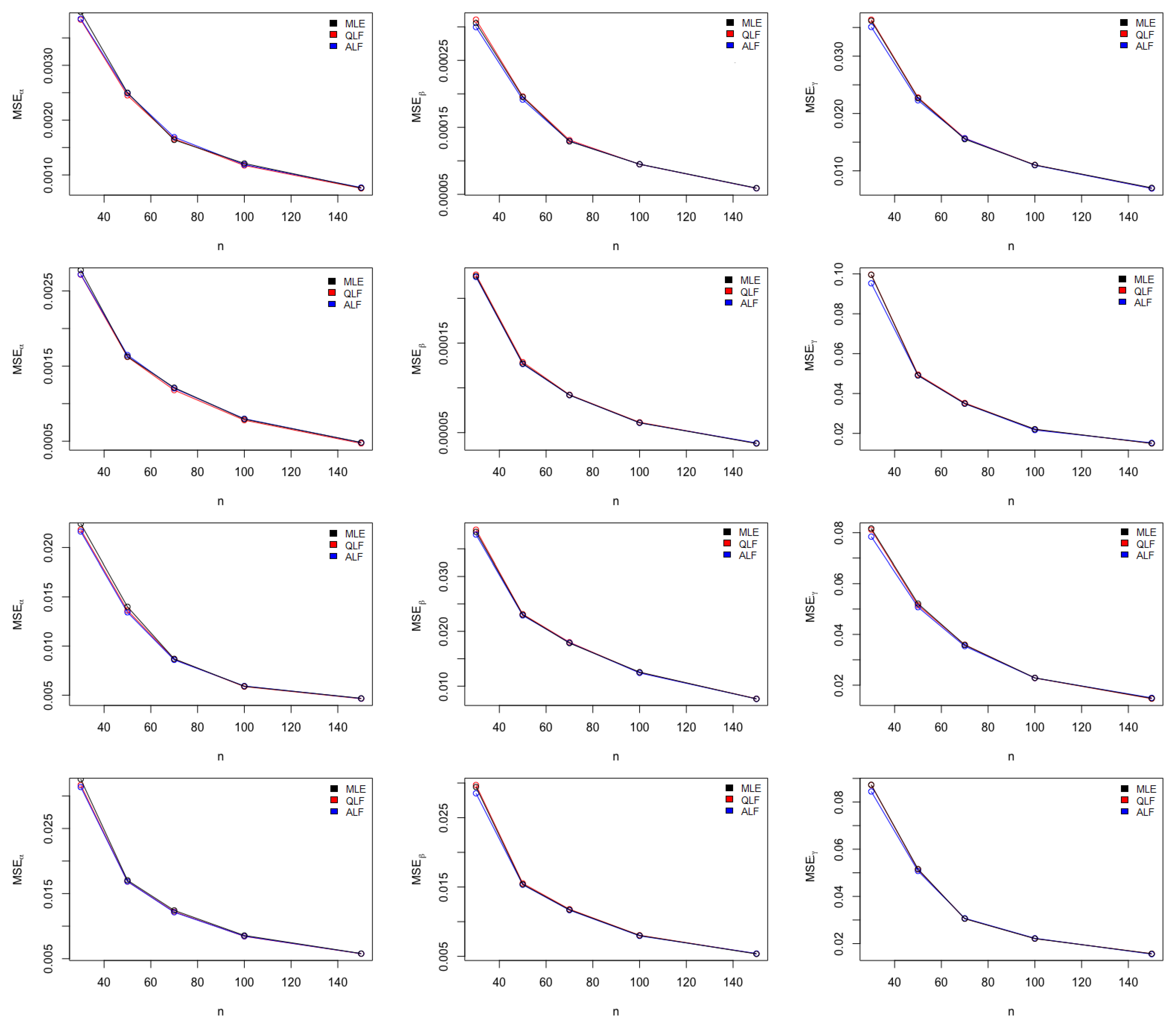
5.2. Simulation Results
5.3. Discussion of Simulation Results
6. Applications
6.1. Objectives
6.2. Data Description
- Data I: This dataset consists of mortality rates for 76 independent COVID-19 patients from the United Kingdom. Each observation corresponds to a single patient-level outcome, and no patient contributes more than one observation to the dataset. The data were collected during the period from April 15 to June 30, 2020; this time span specifies the data collection window only and does not imply temporal ordering, serial dependence, or repeated measurements. Consequently, the observations are treated as independent and identically distributed (i.i.d.), which is consistent with the analysis in Kilai et al. [13].
- Data II: This dataset contains remission times, measured in months, for 128 bladder cancer patients. Each observation represents the remission time of an individual patient and is therefore assumed to be independent. The data were analyzed under the i.i.d. framework in Arshad et al. [14] and were originally reported by Lee and Wang [15].
- Data III: The dataset reported by Efron [16] represents the survival times of patients diagnosed with head and neck cancer, and treated using radiotherapy (RT). Each survival time corresponds to a distinct patient, and the observations are conventionally modeled as independent lifetime data.
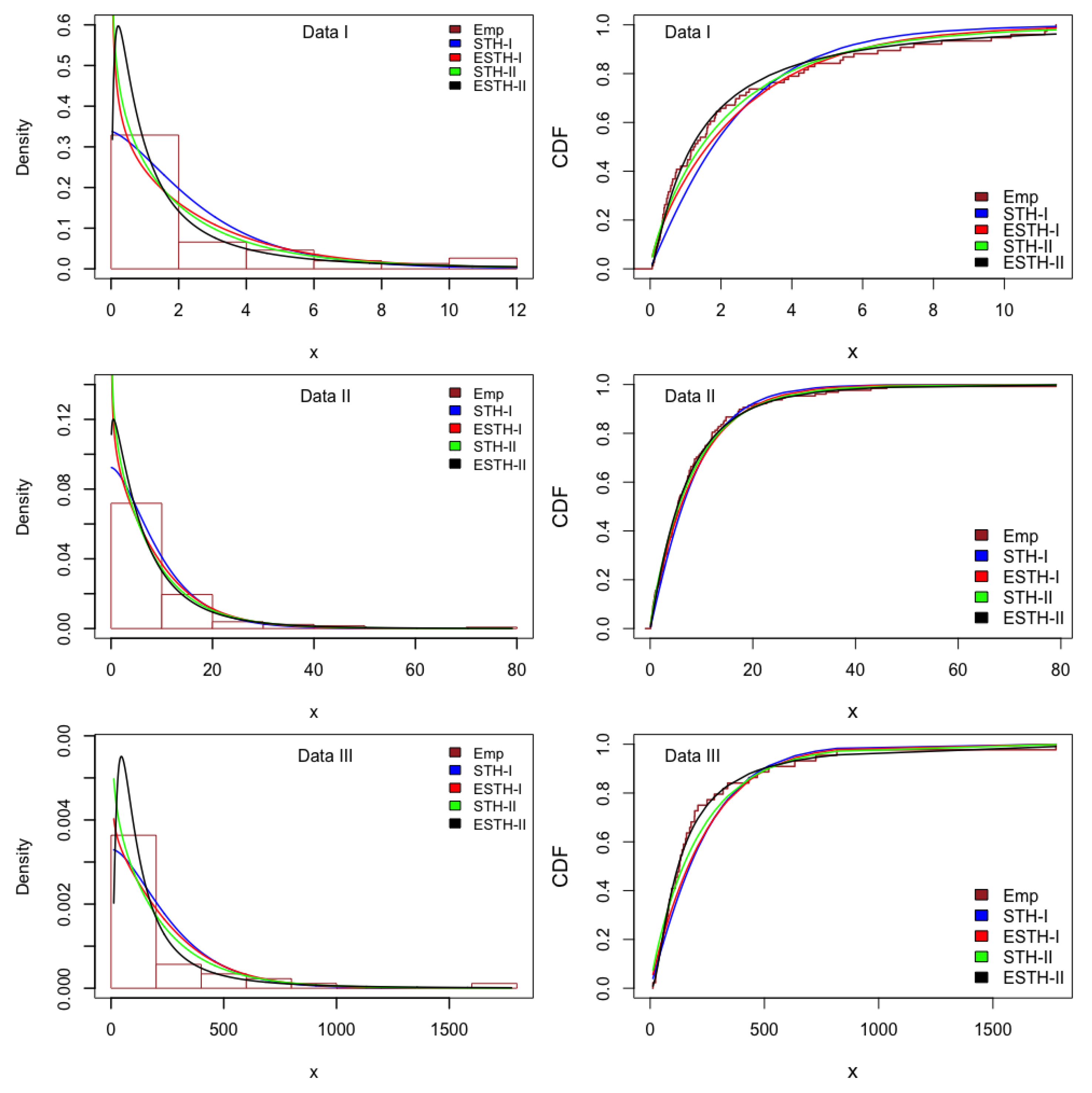
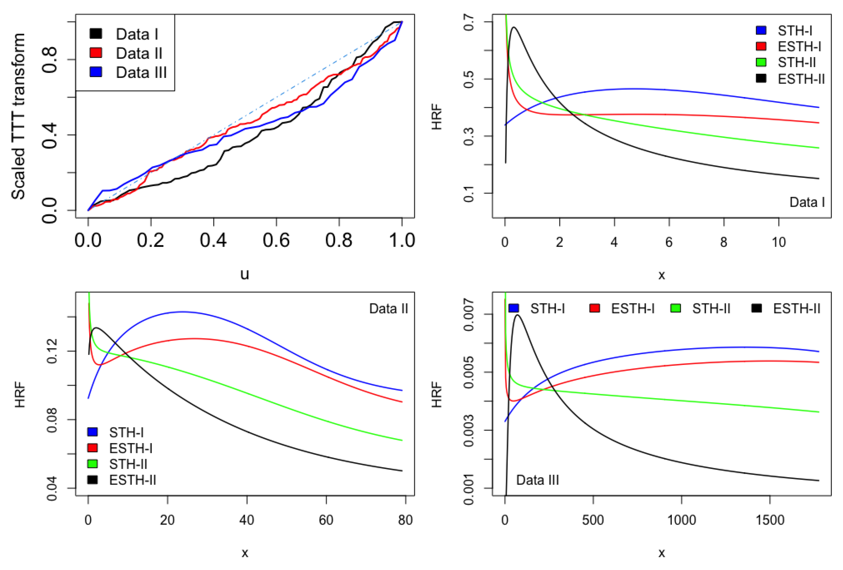
6.3. Results and Analysis
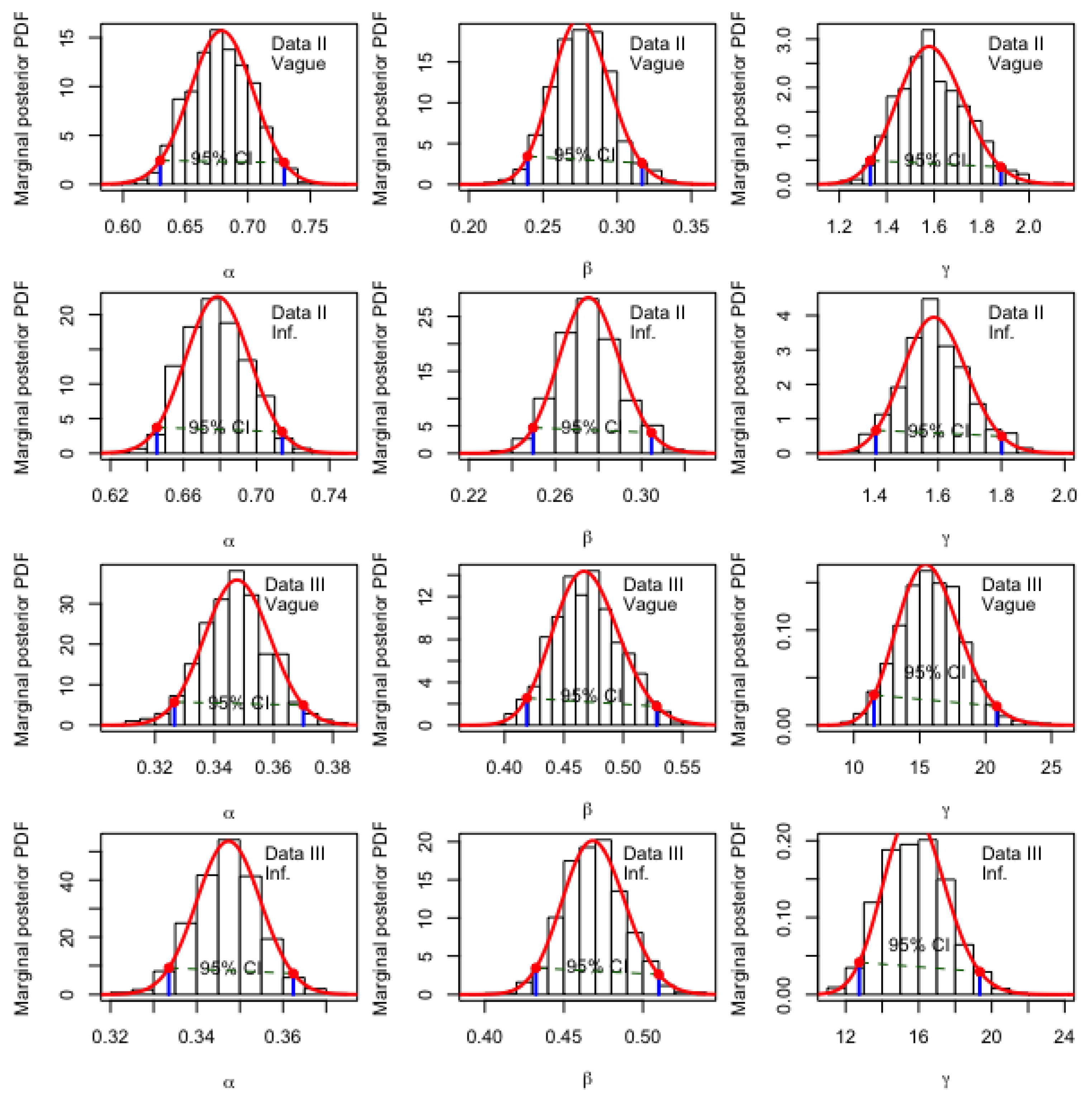
6.4. BayesianInference
- Prior I (the weakly informative prior): for all datasets.
- Prior II (the informative prior):
- (1)
- For Data I: , , , , , and ;
- (2)
- For Data II: , , , , , and ;
- (3)
- For Data III: , , , , , and .
- 1.
- Run m-independent MCMC chains, each of length k (after burn-in), for the model parameters , , and . Let denote the jth draw from chain i for parameter , where and .
- 2.
- Compute the chain means and the overall mean, as follows:
- (a)
- The mean of chain i is
- (b)
- The overall mean is
- 3.
- Compute the average within-chain variance W as follows:
- 4.
- Compute the between-chain variance B as follows:
- 5.
- Estimate the marginal posterior variance as follows:
- 6.
- Compute the Gelman–Rubin statistic as follows:
- 7.
- Repeat Steps 2–6 for the remaining parameters and .
7. Conclusions and Future Work
Author Contributions
Funding
Institutional Review Board Statement
Data Availability Statement
Conflicts of Interest
Appendix A
- The CDF of the exponentiated Lindely (EL) distribution follows (see Nadarajah et al. [3]):
- The CDF of the exponentiated quasi Lindley (EQL) distribution follows (see Elbatal et al. [4]):
- The CDF of the exponentiated XLindley (EXL) distribution follows (see Alomair et al. [5]):
- The CDF of the exponentiated Power Lindley (EPL) distribution follows (see Ashour et al. [6]):
Appendix B
Appendix C
Appendix C.1. Data
- Data I “COVID-19 Mortality Data”:
- 11.2019, 0.411, 2.136, 0.5837, 7.0657, 1.1305, 9.6315, 0.2992, 0.2079, 10.187, 2.4153, 0.6365, 4.1969, 0.2751, 1.6998, 3.3715, 2.7946, 0.3553, 1.1468, 1.2707, 1.6083, 0.2395, 0.5696, 1.8721, 0.4954, 1.6324, 4.3451, 1.3423, 11.1429, 3.9042, 4.6477, 5.45, 1.6017, 0.0587, 1.8164, 11.4584, 0.1247, 0.1165, 0.5139, 1.5709, 0.0863, 0.7096, 0.3446, 0.859, 1.9844, 0.7193, 0.3622, 4.4627, 1.226, 0.6197, 3.784, 0.3317, 6.4241, 1.4149, 0.469, 0.1277, 2.7087, 2.3987, 0.3926, 1.8392, 1.1533, 0.2845, 1.0438, 0.4633, 0.3926, 0.3188, 0.7444, 3.3609, 5.7522, 5.3664, 1.0602, 0.1303, 2.5225, 7.4456, 8.2307, 0.1652
- Data II “Remission Times”:
- 9.02 4.26 4.51 17.14 6.76 5.32 6.39 0.52 7.87 2.69 19.13 2.46 3.48 5.06 18.1 1.05 0.51 1.76 0.9 2.54 2.87 10.34 2.64 25.74 5.85 5.17 12.63 3.57 0.66 5.71 4.5 36.66 2.26 7.09 3.36 0.22 3.7 22.69 0.08 0.73 4.4 5.09 46.12 0.96 5.49 10.75 11.98 7.28 43.01 13.29 17.36 2.02 0.26 12.07 13.11 11.64 14.38 4.98 0.82 11.25 3.46 5.34 6.54 3.25 16.62 9.74 1.35 14.24 0.62 9.47 8.66 14.77 2.83 0.2 13.8 7.26 3.36 10.06 26.31 2.23 23.63 5.32 6.97 0.81 8.53 0.19 4.33 0.5 8.65 11.79 0.4 2.09 2.07 7.32 4.87 2.69 20.28 0.39 14.76 0.4 34.26 7.63 8.37 79.05 7.62 7.59 3.02 3.28 7.93 5.41 6.25 10.66 2.75 1.46 4.34 6.94 4.18 0.31 32.15 5.41 1.26 4.23 5.62 2.02 17.12 3.88 12.03 12.02
- Data III “Survival Times”:
- 25.87 519 339 12.2 633 130 469 58.36 194 817 110 63.47 146 47.38 68.46 23.74 432 140 112 725 179 74.47 209 23.56 78.26 84 119 155 37 1776 133 127 319 249 195 41.35 55.46 94 92 159 173 81.43 281 31.98
Appendix C.2. R Codes
References
- Sarhan, A.M.; Tadj, L.; Hamilton, D.C. A new lifetime distribution and its power transformation. J. Probab. Stat. 2014, 532024. [Google Scholar] [CrossRef] [Scilit]
- Gupta, R.D.; Kundu, D. Theory & methods: Generalized exponential distributions. Aust. N. Z. J. Stat. 1999, 41, 173–188. [Google Scholar]
- Nadarajah, S.; Bakouch, H.S.; Tahmasbi, R. A generalized Lindley distribution. Sankhya B 2011, 73, 331–359. [Google Scholar] [CrossRef] [Scilit]
- Elbatal, I.; Diab, L.S.; Elgarhy, M. Exponentiated quasi Lindley distribution. Int. J. Reliab. Appl. 2016, 17, 1–19. [Google Scholar]
- Alomair, A.M.; Ahmed, M.; Tariq, S.; Ahsan-ul-Haq, M.; Talib, J. An exponentiated XLindley distribution with properties, inference and applications. Heliyon 2024, 10, e25472. [Google Scholar] [CrossRef] [Scilit] [PubMed]
- Ashour, S.K.; Eltehiwy, M.A. Exponentiated power Lindley distribution. J. Adv. Res. 2015, 6, 895–905. [Google Scholar] [CrossRef] [Scilit] [PubMed]
- Abramowitz, M.; Stegun, I.A. Handbook of Mathematical Functions; Dover: Garden City, NY, USA, 1964. [Google Scholar]
- Casella, G.; Berger, R.L. Statistical Inference, 2nd ed.; Duxbury: New York, NY, USA, 2002. [Google Scholar]
- Kalbfleisch, J.G. Probability and Statistical Inference: Volume 2, Statistical Inference, 2nd ed.; Springer-Verlag: Berlin/Heidelberg, Germany, 1985. [Google Scholar]
- Gelman, A.; Brooks, S.; Jones, G. Handbook of Markov Chain Monte Carlo; Chapman and Hall/CRC: Boca Raton, FL, USA, 2011. [Google Scholar]
- Chib, S.; Greenberg, E. Understanding the Metropolis–Hastings algorithm. Am. Stat. 1995, 49, 327–335. [Google Scholar] [CrossRef] [Scilit]
- Gelman, A.; Rubin, D.B. Inference from iterative simulation using multiple sequences. Stat. Sci. 1992, 7, 457–472. [Google Scholar] [CrossRef] [Scilit]
- Kilai, M.; Gichuhi, A.; Kibira, A.W.; Alshanbari, H.M.; El-Morshedy, M. A new generalization of Gull Alpha Power Family of distributions with application to modeling COVID-19 mortality rates. Results Phys. 2022, 36, 105339. [Google Scholar] [CrossRef] [Scilit] [PubMed]
- Arshad, M.Z.; Iqbal, M.Z.; Mutairi, A.A. A comprehensive review of datasets for statistical research in probability and quality control. J. Math. Comput. Sci. 2021, 11, 3663–3728. [Google Scholar] [CrossRef] [Scilit]
- Lee, E.T.; Wang, J.W. Statistical Methods for Survival Data Analysis, 3rd ed.; Wiley: New York, NY, USA, 2003. [Google Scholar]
- Efron, B. Logistic regression, survival analysis, and the Kaplan–Meier curve. J. Am. Stat. Assoc. 1988, 83, 414–425. [Google Scholar] [CrossRef]



| 1.0 | 1.035 | 2.917 | 13.5 | 89.5 | 1.845 | 2.662 | 14.3 | 0.875 | 1.500 | 3.938 | 14.3 | 0.734 | 2.129 | 10.4 | 0.684 | 0.728 | 1.086 | 2.124 | 0.260 | 1.742 | 7.989 |
| 1.5 | 0.865 | 1.363 | 2.917 | 7.76 | 0.614 | 1.404 | 5.6 | 0.831 | 0.989 | 1.500 | 2.743 | 0.299 | 1.107 | 4.757 | 0.734 | 0.670 | 0.728 | 0.920 | 0.131 | 0.943 | 4.362 |
| 2.0 | 0.829 | 1.035 | 1.610 | 2.92 | 0.348 | 0.850 | 3.57 | 0.835 | 0.875 | 1.076 | 1.500 | 0.178 | 0.639 | 3.437 | 0.775 | 0.684 | 0.673 | 0.728 | 0.083 | 0.571 | 3.461 |
| 2.5 | 0.824 | 0.917 | 1.209 | 1.79 | 0.238 | 0.516 | 2.86 | 0.847 | 0.840 | 0.935 | 1.139 | 0.123 | 0.354 | 2.999 | 0.806 | 0.709 | 0.672 | 0.679 | 0.059 | 0.347 | 3.152 |
| 3.0 | 0.828 | 0.865 | 1.035 | 1.36 | 0.179 | 0.282 | 2.58 | 0.860 | 0.831 | 0.875 | 0.989 | 0.091 | 0.156 | 2.856 | 0.831 | 0.734 | 0.684 | 0.670 | 0.044 | 0.195 | 3.042 |
| 3.5 | 0.836 | 0.841 | 0.946 | 1.15 | 0.142 | 0.104 | 2.48 | 0.872 | 0.831 | 0.848 | 0.915 | 0.071 | 0.008 | 2.836 | 0.850 | 0.756 | 0.701 | 0.674 | 0.034 | 0.083 | 3.013 |
| 4.0 | 0.844 | 0.829 | 0.896 | 1.04 | 0.117 | -0.037 | 2.48 | 0.882 | 0.835 | 0.835 | 0.875 | 0.057 | -0.108 | 2.872 | 0.865 | 0.775 | 0.718 | 0.684 | 0.027 | -0.002 | 3.021 |
| 4.5 | 0.852 | 0.825 | 0.865 | 0.964 | 0.098 | -0.153 | 2.52 | 0.891 | 0.841 | 0.831 | 0.853 | 0.047 | -0.201 | 2.937 | 0.877 | 0.792 | 0.734 | 0.696 | 0.022 | -0.070 | 3.046 |
| 5.0 | 0.860 | 0.824 | 0.847 | 0.917 | 0.084 | -0.251 | 2.59 | 0.899 | 0.847 | 0.830 | 0.840 | 0.039 | -0.279 | 3.014 | 0.888 | 0.806 | 0.749 | 0.709 | 0.019 | -0.125 | 3.079 |
| 1.0 | 0.818 | 7.241 | 191.9 | 10283.5 | 6.572 | 10.4 | 224.2 | 0.875 | 1.500 | 3.938 | 14.25 | 0.734 | 2.129 | 10.4 | 1.071 | 1.301 | 1.760 | 2.616 | 0.155 | 0.582 | 3.556 |
| 1.5 | 0.387 | 1.626 | 19.82 | 478.5 | 1.476 | 10.1 | 206.1 | 0.600 | 0.711 | 1.289 | 3.200 | 0.351 | 2.119 | 10.2 | 0.887 | 0.894 | 1.005 | 1.242 | 0.108 | 0.578 | 3.502 |
| 2.0 | 0.227 | 0.556 | 3.880 | 53.1 | 0.504 | 9.8 | 195.3 | 0.458 | 0.417 | 0.578 | 1.094 | 0.207 | 2.106 | 10.0 | 0.775 | 0.684 | 0.673 | 0.728 | 0.083 | 0.571 | 3.461 |
| 2.5 | 0.149 | 0.240 | 1.083 | 9.518 | 0.218 | 9.7 | 188.1 | 0.371 | 0.274 | 0.309 | 0.472 | 0.136 | 2.094 | 9.86 | 0.698 | 0.555 | 0.492 | 0.480 | 0.068 | 0.564 | 3.431 |
| 3.0 | 0.106 | 0.120 | 0.379 | 2.321 | 0.109 | 9.6 | 183.1 | 0.313 | 0.194 | 0.184 | 0.236 | 0.097 | 2.085 | 9.76 | 0.640 | 0.467 | 0.380 | 0.340 | 0.057 | 0.559 | 3.408 |
| 3.5 | 0.079 | 0.067 | 0.156 | 0.701 | 0.060 | 9.5 | 179.3 | 0.270 | 0.145 | 0.119 | 0.131 | 0.072 | 2.076 | 9.67 | 0.595 | 0.404 | 0.305 | 0.254 | 0.050 | 0.554 | 3.390 |
| 4.0 | 0.061 | 0.040 | 0.072 | 0.248 | 0.036 | 9.42 | 176.4 | 0.237 | 0.113 | 0.081 | 0.079 | 0.056 | 2.070 | 9.61 | 0.558 | 0.355 | 0.252 | 0.197 | 0.044 | 0.550 | 3.375 |
| 4.5 | 0.049 | 0.025 | 0.036 | 0.099 | 0.023 | 9.36 | 174.1 | 0.212 | 0.090 | 0.058 | 0.050 | 0.045 | 2.064 | 9.55 | 0.527 | 0.317 | 0.213 | 0.157 | 0.039 | 0.547 | 3.363 |
| 5.0 | 0.040 | 0.017 | 0.020 | 0.043 | 0.015 | 9.32 | 172.2 | 0.192 | 0.073 | 0.042 | 0.033 | 0.037 | 2.059 | 9.51 | 0.501 | 0.287 | 0.183 | 0.128 | 0.036 | 0.544 | 3.353 |
| 1.0 | 5.330 | 176.000 | 17280.000 | 3575040.100 | 147.600 | 8.300 | 148.500 | 0.875 | 1.500 | 3.940 | 14.251 | 0.734 | 2.129 | 10.401 | 0.602 | 0.458 | 0.410 | 0.417 | 0.095 | 0.650 | 3.401 |
| 1.5 | 7.421 | 259.901 | 25844.800 | 5359651.511 | 204.912 | 7.120 | 111.220 | 1.115 | 2.090 | 5.700 | 21.100 | 0.849 | 1.911 | 9.100 | 0.704 | 0.585 | 0.553 | 0.582 | 0.089 | 0.586 | 3.420 |
| 2.0 | 9.261 | 341.611 | 34362.600 | 7142371.300 | 255.910 | 6.471 | 92.000 | 1.301 | 2.616 | 7.389 | 27.680 | 0.922 | 1.79 | 8.45 | 0.775 | 0.684 | 0.673 | 0.728 | 0.083 | 0.571 | 3.462 |
| 2.5 | 10.920 | 421.200 | 42835.711 | 8923232.500 | 302.000 | 6.031 | 80.211 | 1.454 | 3.090 | 8.983 | 34.142 | 0.975 | 1.716 | 8.074 | 0.829 | 0.766 | 0.778 | 0.861 | 0.079 | 0.570 | 3.499 |
| 3.0 | 12.441 | 499.000 | 51265.700 | 10702266.300 | 344.311 | 5.710 | 72.100 | 1.584 | 3.520 | 10.505 | 40.458 | 1.016 | 1.667 | 7.82 | 0.871 | 0.835 | 0.871 | 0.983 | 0.076 | 0.576 | 3.530 |
| 3.5 | 13.800 | 575.100 | 59654.600 | 12479502.300 | 383.600 | 5.470 | 66.110 | 1.696 | 3.930 | 12.000 | 46.600 | 1.050 | 1.630 | 7.630 | 0.906 | 0.895 | 0.955 | 1.095 | 0.073 | 0.582 | 3.555 |
| 4.0 | 15.100 | 649.700 | 68003.800 | 14254968.500 | 420.400 | 5.270 | 61.500 | 1.796 | 4.300 | 13.400 | 52.700 | 1.080 | 1.602 | 7.490 | 0.936 | 0.948 | 1.031 | 1.200 | 0.071 | 0.589 | 3.576 |
| 4.5 | 16.400 | 722.800 | 76314.600 | 16028691.700 | 455.000 | 5.110 | 57.900 | 1.890 | 4.650 | 14.700 | 58.600 | 1.098 | 1.580 | 7.370 | 0.963 | 0.995 | 1.100 | 1.300 | 0.069 | 0.596 | 3.594 |
| 5.0 | 17.500 | 794.600 | 84588.600 | 17800697.400 | 487.800 | 4.970 | 54.900 | 1.970 | 4.980 | 16.100 | 64.500 | 1.120 | 1.560 | 7.300 | 0.986 | 1.038 | 1.166 | 1.390 | 0.067 | 0.603 | 3.609 |
| MLE | QLF | ALF | MLE | QLF | ALF | ||||||||||||||
| Par. | APE | MSE | CP | APE | MSE | CP | APE | MSE | CP | APE | MSE | CP | APE | MSE | CP | APE | MSE | CP | |
| 30 | 1.008 | 0.0040 | 94.6 | 1.0013 | 0.0038 | 94.3 | 1.0027 | 0.0038 | 94.3 | 1.0038 | 0.0028 | 94.8 | 0.9987 | 0.0027 | 94.2 | 0.9994 | 0.0027 | 94.2 | |
| 0.102 | 0.0003 | 95.1 | 0.1024 | 0.0003 | 93.9 | 0.1013 | 0.00034 | 93.9 | 0.1008 | 0.0002 | 94.4 | 0.1012 | 0.0002 | 94.3 | 0.1004 | 0.0002 | 94.3 | ||
| 1.038 | 0.0362 | 95.6 | 1.0386 | 0.0364 | 95.1 | 1.0273 | 0.0351 | 95.1 | 1.5691 | 0.0995 | 95.3 | 1.57 | 0.0996 | 93.2 | 1.5521 | 0.0953 | 93.2 | ||
| 50 | 1.0058 | 0.0025 | 94.0 | 1.0017 | 0.0025 | 92.3 | 1.0024 | 0.0025 | 92.3 | 1.0036 | 0.0016 | 95.7 | 1.0007 | 0.0016 | 94.4 | 1.001 | 0.0016 | 94.4 | |
| 0.1014 | 0.0002 | 94.7 | 0.1016 | 0.0002 | 93.5 | 0.101 | 0.0002 | 93.5 | 0.101 | 0.0001 | 95.3 | 0.1012 | 0.0001 | 94.5 | 0.1008 | 0.0001 | 94.5 | ||
| 1.0287 | 0.0227 | 95.2 | 1.0289 | 0.0228 | 93.3 | 1.0221 | 0.0223 | 93.3 | 1.5313 | 0.0491 | 95.7 | 1.531 | 0.0495 | 94.7 | 1.5206 | 0.0490 | 94.7 | ||
| 70 | 1.0051 | 0.0016 | 95.2 | 1.0022 | 0.0017 | 94.3 | 1.0026 | 0.0017 | 94.3 | 1.0045 | 0.0012 | 94.2 | 1.0026 | 0.0012 | 93.2 | 1.0028 | 0.0012 | 93.2 | |
| 0.1014 | 0.00014 | 96.6 | 0.1016 | 0.0001 | 93.8 | 0.1011 | 0.0001 | 93.8 | 0.1011 | 0.0001 | 95.4 | 0.1012 | 0.0001 | 94.9 | 0.1009 | 0.0001 | 94.9 | ||
| 1.0102 | 0.0155 | 94.7 | 1.011 | 0.0157 | 93.0 | 1.0071 | 0.0157 | 93.0 | 1.5249 | 0.0350 | 96.0 | 1.5262 | 0.0353 | 93.4 | 1.5189 | 0.0349 | 93.4 | ||
| 100 | 1.003 | 0.0012 | 94.4 | 1.001 | 0.0012 | 92.7 | 1.0012 | 0.0012 | 92.7 | 1.0032 | 0.0008 | 95.2 | 1.0016 | 0.0008 | 93.0 | 1.0015 | 0.0008 | 93.0 | |
| 0.1008 | 0.0001 | 94.1 | 0.1009 | 0.0001 | 93.2 | 0.1006 | 0.0001 | 93.2 | 0.1008 | 0.0001 | 95.9 | 0.1009 | 0.0001 | 93.8 | 0.1007 | 0.0001 | 93.8 | ||
| 1.0111 | 0.0110 | 95.2 | 1.0115 | 0.0110 | 93.3 | 1.0081 | 0.0110 | 93.3 | 1.5122 | 0.0221 | 95.8 | 1.5125 | 0.0220 | 93.9 | 1.5066 | 0.0217 | 93.9 | ||
| 150 | 1.003 | 0.0008 | 95.1 | 1.0017 | 0.0008 | 91.7 | 1.0019 | 0.0008 | 91.7 | 1.0008 | 0.0005 | 96.1 | 1.0000 | 0.0005 | 93.7 | 1.0002 | 0.0005 | 93.7 | |
| 0.1008 | 0.0001 | 94.7 | 0.1008 | 0.0001 | 93.8 | 0.1005 | 0.0001 | 93.8 | 0.1003 | 0 | 96.1 | 0.1003 | 0 | 94.5 | 0.1001 | 0 | 94.5 | ||
| 1.0079 | 0.0070 | 95.5 | 1.0091 | 0.0069 | 93.4 | 1.0068 | 0.0069 | 93.4 | 1.5075 | 0.0150 | 95.0 | 1.5083 | 0.0150 | 93.8 | 1.5046 | 0.0152 | 93.8 | ||
| = (1, 1.2, 1.5) | |||||||||||||||||||
| MLE | QLF | ALF | MLE | QLF | ALF | ||||||||||||||
| APE | MSE | CP | APE | MSE | CP | APE | MSE | CP | APE | MSE | CP | APE | MSE | CP | APE | MSE | CP | ||
| 30 | 1.0239 | 0.0224 | 95.0 | 1.0166 | 0.0218 | 94.7 | 1.0125 | 0.0216 | 94.7 | 1.2303 | 0.0326 | 94.8 | 1.2201 | 0.0317 | 93.3 | 1.2157 | 0.0314 | 93.3 | |
| 1.2164 | 0.0381 | 94.5 | 1.2222 | 0.0385 | 95.7 | 1.2101 | 0.0376 | 95.7 | 1.0242 | 0.0294 | 93.0 | 1.0296 | 0.0297 | 93.7 | 1.0188 | 0.0285 | 93.7 | ||
| 1.5522 | 0.0817 | 96.1 | 1.5512 | 0.0812 | 95.4 | 1.5339 | 0.0784 | 95.4 | 1.5451 | 0.0873 | 96.0 | 1.5450 | 0.0872 | 95.7 | 1.5270 | 0.0845 | 95.7 | ||
| 50 | 1.0209 | 0.0140 | 94.8 | 1.0164 | 0.0136 | 94.1 | 1.0140 | 0.0134 | 94.1 | 1.2186 | 0.0170 | 95.4 | 1.2122 | 0.0168 | 94.5 | 1.2100 | 0.0169 | 94.5 | |
| 1.2088 | 0.0230 | 94.4 | 1.2118 | 0.0231 | 94.4 | 1.2045 | 0.0229 | 94.4 | 1.0093 | 0.0154 | 94.7 | 1.0126 | 0.0155 | 95.1 | 1.0061 | 0.0153 | 95.1 | ||
| 1.5433 | 0.0521 | 94.8 | 1.5419 | 0.0515 | 93.3 | 1.5325 | 0.0507 | 93.3 | 1.5367 | 0.0516 | 95.1 | 1.5373 | 0.0515 | 94.7 | 1.5274 | 0.0508 | 94.7 | ||
| 70 | 1.0081 | 0.0087 | 95.0 | 1.0050 | 0.0087 | 94.5 | 1.0029 | 0.0086 | 94.5 | 1.2197 | 0.0124 | 94.4 | 1.2148 | 0.0122 | 94.0 | 1.2130 | 0.0121 | 94.0 | |
| 1.2093 | 0.0178 | 94.6 | 1.2123 | 0.0180 | 94.0 | 1.2072 | 0.0179 | 94.0 | 1.0128 | 0.0117 | 94.4 | 1.0152 | 0.0118 | 94.4 | 1.0107 | 0.0117 | 94.4 | ||
| 1.5224 | 0.0359 | 95.2 | 1.5227 | 0.0359 | 93.5 | 1.5156 | 0.0354 | 93.5 | 1.5179 | 0.0305 | 95.6 | 1.5177 | 0.0306 | 95.2 | 1.5109 | 0.0307 | 95.2 | ||
| 100 | 1.0018 | 0.0059 | 94.9 | 0.9993 | 0.0059 | 94.0 | 0.9982 | 0.0059 | 94.0 | 1.2080 | 0.0086 | 95.0 | 1.2045 | 0.0084 | 94.9 | 1.2033 | 0.0085 | 94.9 | |
| 1.2048 | 0.0126 | 94.5 | 1.2067 | 0.0125 | 94.3 | 1.2030 | 0.0124 | 94.3 | 1.0055 | 0.0080 | 95.0 | 1.0068 | 0.0080 | 93.8 | 1.0034 | 0.0079 | 93.8 | ||
| 1.5120 | 0.0229 | 95.3 | 1.5118 | 0.0228 | 94.0 | 1.5068 | 0.0228 | 94.0 | 1.5138 | 0.0221 | 95.6 | 1.5138 | 0.0221 | 94.1 | 1.5086 | 0.0223 | 94.1 | ||
| 150 | 1.0071 | 0.0047 | 93.5 | 1.0054 | 0.0046 | 92.8 | 1.0045 | 0.0047 | 92.8 | 1.2063 | 0.0058 | 93.8 | 1.2041 | 0.0058 | 93.1 | 1.2033 | 0.0058 | 93.1 | |
| 1.2058 | 0.0077 | 95.5 | 1.2070 | 0.0077 | 94.4 | 1.2048 | 0.0077 | 94.4 | 1.0064 | 0.0053 | 94.9 | 1.0073 | 0.0054 | 93.7 | 1.0054 | 0.0054 | 93.7 | ||
| 1.5076 | 0.0148 | 94.8 | 1.5070 | 0.0147 | 93.5 | 1.5046 | 0.0150 | 93.5 | 1.5069 | 0.0157 | 94.7 | 1.5062 | 0.0157 | 93.2 | 1.5017 | 0.0155 | 93.2 | ||
| Model | (SE) | (SE) | (SE) | AIC | K-S | p-Value | |||
|---|---|---|---|---|---|---|---|---|---|
| Data I | |||||||||
| STH-I | 0.3387 (0.0418) | - | - | −146.6420 | 295.2841 | 1.0881 | 0.1657 | 0.1694 | 0.0255 |
| ESTH-I | 0.7128 (0.1053) | - | 0.2607 (0.0451) | −143.9384 | 291.8769 | 1.1438 | 0.1749 | 0.1050 | 0.3716 |
| STH-II | 0.7855 (0.0693) | 0.4562 (0.0677) | - | −142.4348 | 288.8697 | 0.8164 | 0.1213 | 0.0797 | 0.7203 |
| EL | 0.4998 (0.0674) | - | 0.6172 (0.0929) | −145.3657 | 294.7314 | 1.4137 | 0.2192 | 0.1111 | 0.3045 |
| EQL | 0.3681 (0.0792) | 21.6017 (81.7220) | 0.7996 (0.1171) | −142.5148 | 291.0296 | 0.9318 | 0.1400 | 0.0986 | 0.4505 |
| EXL | 0.4778 (0.0626) | - | 0.7092 (0.1076) | −144.0222 | 292.0444 | 1.2099 | 0.1856 | 0.1055 | 0.3663 |
| EPL | 0.7326 (1.2454) | 0.576 (0.1378) | 1.8578 (8.3797) | −139.9435 | 285.887 | 0.3535 | 0.0501 | 0.0569 | 0.9663 |
| ESTH-II | 0.3579 | 2.0223 | 7.0935 | −139.934 | 285.869 | 0.3555 | 0.0509 | 0.0559 | 0.9714 |
| Data II | |||||||||
| STH-I | 0.0925 (0.0078) | - | - | −404.938 | 811.876 | 0.5143 | 0.0742 | 0.0756 | 0.4575 |
| ESTH-I | 0.0813 (0.0949) | - | 0.8243 (0.0098) | −403.484 | 810.968 | 0.5839 | 0.0856 | 0.0609 | 0.7287 |
| STH-II | 0.8492 (0.0571) | 0.1371 (0.0231) | - | −401.726 | 807.452 | 0.3748 | 0.0529 | 0.0511 | 0.8915 |
| EL | 0.1555 (0.0165) | - | 0.5794 (0.0684) | −406.1204 | 816.2407 | 0.8033 | 0.1156 | 0.0779 | 0.4177 |
| EQL | 0.1148 (0.0167) | 25.6046 (65.5004) | 0.9208 (0.1064) | −402.5419 | 811.0837 | 0.4730 | 0.0696 | 0.0552 | 0.8303 |
| EXL | 0.1571 (0.0162) | - | 0.6595 (0.0794) | −405.8700 | 815.7401 | 0.8249 | 0.1215 | 0.0782 | 0.4141 |
| EPL | 0.7326 (0.2914) | 0.5759 (0.1078) | 1.8578 (1.8581) | −400.8387 | 807.6773 | 0.3916 | 0.0591 | 0.0492 | 0.9165 |
| ESTH-II | 0.6801 | 0.2759 | 1.5913 | −400.583 | 807.166 | 0.3396 | 0.0499 | 0.0461 | 0.9483 |
| Data III | |||||||||
| STH-I | 0.003 (0.0004) | - | - | −284.0535 | 570.1071 | 1.1542 | 0.2005 | 0.1809 | 0.0986 |
| ESTH-I | 0.8752 (0.1663) | - | 0.0031 (0.0005) | −283.8067 | 571.6135 | 1.1829 | 0.2057 | 0.1673 | 0.1516 |
| STH-II | 0.8204 (0.0777) | 0.0098 (0.0046) | - | −282.3783 | 568.7567 | 0.8925 | 0.1537 | 0.1256 | 0.4549 |
| EL | 0.0058 (0.0011) | - | 0.4998 (0.1008) | −283.0355 | 570.0711 | 1.0423 | 0.1799 | 0.1626 | 0.1746 |
| EQL | 0.0052 (0.0010) | 9.9409 (13.4971) | 1.0789 (0.2229) | −282.0996 | 570.1991 | 0.8996 | 0.1549 | 0.1512 | 0.2415 |
| EXL | 0.0059 (0.0011) | - | 0.5144 (0.1029) | −283.1906 | 570.3811 | 1.0599 | 0.1828 | 0.1659 | 0.1581 |
| EPL | 1.2948 (1.2365) | 0.2698 (0.1182) | 25.7942 (49.5767) | −277.5244 | 561.0487 | 0.1228 | 0.0191 | 0.0593 | 0.9953 |
| ESTH-II | 0.3481 | 0.4684 | 15.8227 | −277.3516 | 560.7032 | 0.1159 | 0.0175 | 0.0559 | 0.9979 |
| Data | vs. | df | p-Value | |||
|---|---|---|---|---|---|---|
| I | (STH-I) | vs. | (ESTH-I) | 1 | 5.407 | 0.0201 |
| (STH-I) | vs. | (ESTH-II) | 2 | 13.416 | 0.0012 | |
| (ESTH-I) | vs. | (ESTH-II) | 1 | 8.008 | 0.0047 | |
| (STH-II) | vs. | (ESTH-II) | 1 | 5.001 | 0.0253 | |
| II | (STH-I) | vs. | (ESTH-I) | 1 | 2.908 | 0.0881 |
| (STH-I) | vs. | (ESTH-II) | 2 | 8.71 | 0.0128 | |
| (ESTH-I) | vs. | (ESTH-II) | 1 | 5.801 | 0.0160 | |
| (STH-II) | vs. | (ESTH-II) | 1 | 2.286 | 0.1306 | |
| III | (STH-I) | vs. | (ESTH-I) | 1 | 0.497 | 0.4807 |
| (STH-I) | vs. | (ESTH-II) | 2 | 13.407 | 0.0012 | |
| (ESTH-I) | vs. | (ESTH-II) | 1 | 12.909 | 0.0003 | |
| (STH-II) | vs. | (ESTH-II) | 1 | 10.051 | 0.0015 |
| Bayesian Estimates | Confidence Intervals | ||||
|---|---|---|---|---|---|
| Data | Par. | Weakly Informative Prior | Informative | Asymptotic | Likelihood |
| I | 0.3563 (0.3554) | 0.3573 (0.3565) | |||
| 2.0241 (2.0233) | 2.0224 (2.0189) | ||||
| 7.055 (7.0025) | 7.086 (7.0515) | ||||
| II | 0.6783 (0.6781) | 0.6776 (0.6770) | |||
| 0.2763 (0.2759) | 0.2757 (0.2754) | ||||
| 1.5951 (1.5813) | 1.5900 (1.5862) | ||||
| III | 0.3471 (0.3473) | 0.3471 (0.3474) | |||
| 0.4695 (0.4693) | 0.4691 (0.4679) | ||||
| 15.8795 (15.8048) | 15.7988 (15.7699) | ||||
| Credible Intervals (MCMC) | Exact Credible Intervals | ||||
| Weakly Informative Prior | Informative | Weakly Informative Prior | Informative | ||
| I | |||||
| II | |||||
| III | |||||
| Chain | Mean | Variance | Mean | Variance | Mean | Variance |
| Data I | ||||||
| 1 | 0.3564989 | 0.0004269295 | 2.02334 | 0.007152241 | 7.132806 | 0.3271977 |
| 2 | 0.3563541 | 0.000417599 | 2.024036 | 0.006679194 | 7.120189 | 0.3339793 |
| 3 | 0.3577726 | 0.0004414557 | 2.023744 | 0.006983468 | 7.070339 | 0.3552804 |
| 4 | 0.3583323 | 0.0004080709 | 2.016696 | 0.007076394 | 7.086573 | 0.3478988 |
| 5 | 0.3562034 | 0.0004278291 | 2.025041 | 0.007150677 | 7.100076 | 0.3207258 |
| 6 | 0.3570126 | 0.0004112886 | 2.026344 | 0.00667269 | 7.085031 | 0.2933487 |
| 7 | 0.3564653 | 0.0003857774 | 2.017757 | 0.006998961 | 7.141821 | 0.3232892 |
| 8 | 0.3555877 | 0.0004231039 | 2.016525 | 0.007146827 | 7.110605 | 0.309977 |
| 9 | 0.3570127 | 0.0004160165 | 2.025359 | 0.007346811 | 7.128938 | 0.3478143 |
| 10 | 0.3577661 | 0.0004010358 | 2.017941 | 0.007464367 | 7.075059 | 0.300759 |
| Overall Mean | 0.3569006 | 0.0004159106 | 2.021678 | 0.007067163 | 7.105144 | 0.326027 |
| B | 0.007159882 | 0.1554755 | 6.471491 | |||
| 0.000416585 | 0.007082004 | 0.3266415 | ||||
| 1.00081 | 1.001049 | 1.000942 | ||||
| Data II | ||||||
| 1 | 0.6784543 | 0.0003306328 | 0.2768565 | 0.000208984 | 1.593156 | 0.009165 |
| 2 | 0.6796594 | 0.0003116209 | 0.2756564 | 0.0002080026 | 1.599705 | 0.010285 |
| 3 | 0.6804415 | 0.0002757593 | 0.277311 | 0.0002102146 | 1.590641 | 0.009200 |
| 4 | 0.6790418 | 0.0003251517 | 0.2760122 | 0.0001940104 | 1.585264 | 0.010553 |
| 5 | 0.6786966 | 0.0003789456 | 0.2767015 | 0.0001899971 | 1.589106 | 0.008785 |
| 6 | 0.6800975 | 0.0003474061 | 0.2771244 | 0.000200715 | 1.589256 | 0.009304 |
| 7 | 0.6788874 | 0.0003249929 | 0.2757779 | 0.0002125022 | 1.591236 | 0.008897 |
| 8 | 0.6784231 | 0.000306496 | 0.2766208 | 0.0002044866 | 1.593038 | 0.009305 |
| 9 | 0.6789308 | 0.0003413619 | 0.2761224 | 0.0001986317 | 1.585157 | 0.010066 |
| 10 | 0.6793144 | 0.0003657088 | 0.2755594 | 0.0001962817 | 1.585929 | 0.008804 |
| Overall Mean | 0.6791947 | 0.0003308076 | 0.2763743 | 0.0002023826 | 1.590249 | 0.009436 |
| B | 0.004643392 | 0.003966625 | 0.1983402 | |||
| 0.0003312389 | 0.000202759 | 0.009455271 | ||||
| 1.000652 | 1.00093 | 1.001 | ||||
| Data III | ||||||
| 1 | 0.3477564 | 0.00005954546 | 0.4696218 | 0.0003901486 | 15.7587 | 2.913201 |
| 2 | 0.3483826 | 0.00004775203 | 0.4696503 | 0.00037734 | 15.82331 | 2.727301 |
| 3 | 0.3478268 | 0.00004.881005 | 0.4691026 | 0.0003719368 | 15.72394 | 2.875778 |
| 4 | 0.3482534 | 0.00005.169352 | 0.4701666 | 0.0004067735 | 15.80332 | 2.911068 |
| 5 | 0.3476546 | 0.00004.815847 | 0.470234 | 0.0003833537 | 15.75937 | 2.843547 |
| 6 | 0.347817 | 0.00005.547186 | 0.4692357 | 0.0003968226 | 15.79249 | 2.793001 |
| 7 | 0.3476789 | 0.00005130219 | 0.4693357 | 0.0003678061 | 15.81117 | 2.788853 |
| 8 | 0.3483103 | 0.00005414653 | 0.46988 | 0.000368036 | 15.77399 | 2.872296 |
| 9 | 0.3478863 | 0.00005513234 | 0.4692499 | 0.0004054088 | 15.87618 | 2.736006 |
| 10 | 0.3480249 | 0.00005040109 | 0.4702613 | 0.0003989066 | 15.87353 | 2.961118 |
| Overall Mean | 0.3479591 | 0.00005224135 | 0.4696738 | 0.0003866533 | 15.7996 | 2.842217 |
| B | 0.0007210634 | 0.001955259 | 24.18081 | |||
| 0.00005230824 | 0.0003868101 | 2.844351 | ||||
| 1.00064 | 1.000203 | 1.000375 | ||||
Disclaimer/Publisher’s Note: The statements, opinions and data contained in all publications are solely those of the individual author(s) and contributor(s) and not of MDPI and/or the editor(s). MDPI and/or the editor(s) disclaim responsibility for any injury to people or property resulting from any ideas, methods, instructions or products referred to in the content. |
© 2026 by the authors. Licensee MDPI, Basel, Switzerland. This article is an open access article distributed under the terms and conditions of the Creative Commons Attribution (CC BY) license.
Share and Cite
Manshi, T.; Sarhan, A.M.; Sobh, M.E. Modeling Healthcare Data with a Novel Flexible Three-Parameter Distribution. Mathematics 2026, 14, 359. https://doi.org/10.3390/math14020359
Manshi T, Sarhan AM, Sobh ME. Modeling Healthcare Data with a Novel Flexible Three-Parameter Distribution. Mathematics. 2026; 14(2):359. https://doi.org/10.3390/math14020359
Chicago/Turabian StyleManshi, Thamer, Ammar M. Sarhan, and M. E. Sobh. 2026. "Modeling Healthcare Data with a Novel Flexible Three-Parameter Distribution" Mathematics 14, no. 2: 359. https://doi.org/10.3390/math14020359
APA StyleManshi, T., Sarhan, A. M., & Sobh, M. E. (2026). Modeling Healthcare Data with a Novel Flexible Three-Parameter Distribution. Mathematics, 14(2), 359. https://doi.org/10.3390/math14020359