CNL-Diff: A Nonlinear Data Transformation Framework for Epidemic Scale Prediction Based on Diffusion Models

Abstract

In recent years, the complexity and suddenness of infectious disease transmission have posed significant limitations for traditional time-series forecasting methods when dealing with the nonlinearity, non-stationarity, and multi-peak distributions of epidemic scale variations. To address this challenge, this paper proposes a forecasting framework based on diffusion models, called CNL-Diff, aimed at tackling the prediction challenges in complex dynamics, nonlinearity, and non-stationary distributions. Traditional epidemic forecasting models often rely on fixed linear assumptions, which limit their ability to accurately predict the incidence scale of infectious diseases. The CNL-Diff framework integrates a forward–backward consistent conditioning mechanism and nonlinear data transformations, enabling it to capture the intricate temporal and feature dependencies inherent in epidemic data. The results show that this method outperforms baseline models in metrics such as Mean Absolute Error (MAE), Continuous Ranked Probability Score (CRPS), and Prediction Interval Coverage Probability (PICP). This study demonstrates the potential of diffusion models in complex-distribution time-series modeling, providing a more reliable probabilistic forecasting tool for public health monitoring, epidemic early warning, and risk decision making.

1. Introduction and Related Work

1.1. Background and Motivation

The outbreak of infectious diseases has become one of the core uncertainties faced by global public health systems. Unlike the early linear transmission paradigm centered on airport transmission, the current epidemic transmission paths are more influenced by the interactions of three mechanisms: social networks, migration trajectories, and occupational exposures. This results in a complex, dynamic pattern of “short-term exponential growth and long-term heavy-tailed distribution”.

Accurate forecasting of epidemic scale (e.g., incidence and related risk indicators) is therefore essential for public health surveillance, resource planning, and timely interventions, especially when the underlying dynamics are nonlinear, non-stationary, and multi-peaked.

In the field of infectious disease modeling and control systems, early warning methods play a crucial role. An efficient early warning system typically relies on the construction of spatiotemporal sequence data, with the core goal being to identify abnormal growth trends. Therefore, early warning methods can essentially be classified as specialized anomaly detection techniques, and their progress is closely tied to the overall development of anomaly detection methods.

With the advancement of artificial intelligence and deep learning technologies, anomaly detection methods have achieved significant theoretical breakthroughs. The mainstream paradigm has gradually shifted from predictive models to reconstruction models, with a greater focus on the specificity and adaptability of data processing. The design of reconstruction models has undergone rapid iterations [1,2,3], resulting in significant improvements in data processing efficiency. Meanwhile, deeper exploration of the intrinsic mechanisms of anomalies [4] has further enhanced the theoretical performance of detection methods [5].

However, recent studies [6,7,8] point out that these theoretically outstanding methods perform suboptimally in practical applications. Research has shown that they are often limited by weak robustness, high deployment complexity, and stringent requirements for data quality and computing resources. In specific early warning tasks, these methods often only achieve moderate performance levels [9].

Diffusion models offer a feasible path to address these challenges. As an efficient generative modeling tool, diffusion models have gained widespread attention in recent years, with their remarkable capabilities being validated across multiple domains, including image generation [10,11], video synthesis [12,13], robotics [14], and cross-modal tasks [15], outperforming traditional generative methods. Based on these successful applications, scholars have begun exploring the potential of diffusion models for time-series prediction, leading to the development of various diffusion architectures specifically designed to address the complex challenges of time-series data [16,17,18,19,20]. These methods are often built on the foundation of conditional diffusion models, such as that reported in [20], which uses future mixed information as a conditional guide; TimeGrad [21], which combines the diffusion process with the hidden state of a recurrent neural network; and CSDI [16], which uses a self-supervised masking strategy to guide the non-autoregressive denoising process. Nevertheless, existing time-series diffusion models have yet to fully explore the structural potential of diffusion models themselves.

Traditional conditional diffusion models typically rely on fixed linear Gaussian noise patterns during training, where noise is added incrementally in the forward process and the reverse process is optimized to fit the forward diffusion path. Conditional information is only introduced in the reverse stage. This approach has two major limitations: first, the forward process lacks learnable capabilities; second, simplifying prior assumptions to an isotropic Gaussian distribution may increase the complexity of the reverse generation process in time-series tasks.

To address this, this paper proposes and evaluates a conditional diffusion model, integrated with nonlinear data transformations, for prediction of the scale of infectious diseases. This framework introduces a learnable nonlinear transformation mechanism with temporal dependencies and a condition integration strategy in the forward process, enabling it to effectively capture the nonlinear dynamics, non-stationary characteristics, and multi-modal distribution patterns exhibited during the development of epidemics.

1.2. Contributions and Practical Relevance

This work aims to provide an uncertainty-aware forecasting tool for infectious disease scale prediction under complex distributions. Our main contributions are described as follows:

• We propose CNL-Diff, a conditional diffusion forecasting framework that introduces a learnable conditional prior in the forward process rather than injecting conditions only during reverse denoising.
• We design a time-dependent nonlinear transformation ($T_{\varphi }(·,t)$) to reduce distributional distortion caused by nonlinearity, non-stationarity, heavy tails, and sudden multi-peak outbreaks, thereby simplifying the reverse generation task.
• We empirically demonstrate improved deterministic accuracy and probabilistic calibration (MAE/MSE/CRPS/PICP/MPIW) on large-scale China CDC statutory infectious disease surveillance data, highlighting the potential of diffusion models for public health monitoring and early warning.

From a public health perspective, beyond point forecasts, the generated predictive distribution enables actionable risk assessment, e.g., with respect to prediction intervals, threshold exceedance probabilities, and peak timing/magnitude uncertainty.

1.3. Paper Organization and Workflow Overview

Figure 1 summarizes the overall workflow and the structure of this manuscript. Section 2 presents the proposed CNL-Diff framework, including the nonlinear forward transformation and the denoising network. Section 3 reports experimental settings and comparisons with representative baselines. Section 4 discusses practical implications, seasonality-related interpretation, and potential sources of prediction discrepancies.

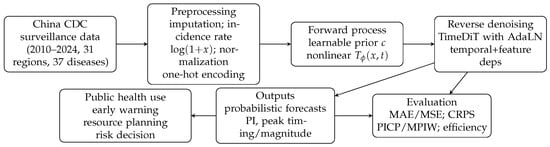
Figure 1. Overall workflow of CNL-Diff for epidemic scale forecasting and the organization of this manuscript.

1.4. Related Work

1.4.1. Anomaly Detection and Early Warning-Specific Models

Early warning and anomaly detection tasks mainly focus on two core methods: one relies on the prediction error generated by predictive models [22], while the other is based on the reconstruction error obtained from reconstruction models [23]. Predictive models forecast future intervals based on early segments of time series, while reconstruction models learn the underlying distribution characteristics by reconstructing the entire sequence. Both strategies are trained on normal samples, so when encountering anomalous patterns, their prediction or reconstruction errors significantly increase, which can be used as a quantitative criterion for detecting abnormal events.

In recent years, reconstruction methods have become the mainstream research paradigm in the anomaly detection field and have received support from various neural network structures, including autoencoders [24,25,26], generative adversarial networks [27,28,29], and diffusion models [30,31,32]. Autoencoders [33] typically consist of an encoder and a decoder, where the encoder maps the input to a low-dimensional latent representation and the decoder reconstructs the original data structure from this representation. Generative adversarial networks [34] involve a generator network and a discriminator network, which form a game: the generator aims to synthesize realistic samples, while the discriminator is responsible for distinguishing between real data and generated results. Diffusion models [10] consist of two key processes: the forward process gradually introduces Gaussian noise to make the data approach a random distribution, while the reverse process iteratively learns to denoise and reconstruct the original data from noise.

The work of Park et al. [25] was one of the earliest studies to systematically apply the reconstruction idea to anomaly detection. They combined long short-term memory [35], a type of recurrent neural network that models long-term dependencies using gating mechanisms, with a variational autoencoder (VAE). The model achieved AUC (Area Under the Receiver Operating Characteristic Curve, a metric that correlates with overall model performance) values of 0.04 and 0.06 on two datasets. Based on this, Pintilie et al. [31] proposed further expansion of the anomaly detection framework by jointly optimizing the autoencoder and diffusion model. The process is described as follows: the autoencoder first reconstructs the test time series; then, noise is added to the reconstructed series, and a diffusion model is used for denoising. The difference between the denoised result and the original sequence is then computed as an anomaly score. Compared to using just the VAE or diffusion model alone, the AUC improves by 0.04.

Although the above architectures have enhanced the utilization of data features through the combination of reconstruction errors, these methods still exhibit significant limitations in terms of generalization performance and are highly dependent on high-quality, large-scale datasets. As a result, they are often only suitable for specific data environments or, in some cases, require multiple customized datasets to achieve optimal performance.

For example, Karadayi et al. [36] designed a reconstruction autoencoder based on Convolutional Long Short-Term Memory (ConvLSTM), a variant of LSTM that incorporates convolution operations to extract spatiotemporal features, specifically for early warning modeling on the Italian COVID-19 dataset. The model demonstrated significant dataset specificity, leading to highly specialized network structures and parameter settings. Since the dataset includes 13 temporal features and 10 spatial features, the method faces significant challenges when being transplanted into other real-world scenarios. Additionally, to adapt the model to this dataset, hierarchical structural adjustments are often required, further emphasizing its specialized nature.

Furthermore, related studies on the nature of anomalies may, in some cases, lead to misleading conclusions. For example, some works use relabeling strategies [1] or similar techniques to extract additional information from the test set. Although these methods may improve certain evaluation metrics, they often do not lead to significant improvements at the practical application level.

1.4.2. Time-Series Forecasting

Time-series forecasting techniques have been widely applied across various fields of daily life, including fundamental scenarios such as traffic flow monitoring, power load analysis, and healthcare management [37], in addition to extensions to more complex tasks like stock price prediction, weather simulation, and wind pattern forecasting [19]. Given its broad application value, research methods in this field have gradually evolved from traditional state-space models to contemporary deep learning frameworks.

In terms of infrastructure expansion, various models demonstrate different technical paths. FiLM [38] combines Fourier analysis and low-rank matrix approximation to reduce noise interference while employing Legendre polynomial projections to maintain the integrity of historical data representations. NBeats [39], as an interpretable architecture, integrates polynomial trend modeling and Fourier-based seasonal detection mechanisms. Its subsequent improved model, Depts [40], adds a periodic sequence processing module, while NHits [41] further enhances performance through a multi-scale hierarchical interpolation strategy.

Some models focus on deep exploration of temporal dependencies. SCINet [42] employs a recursive strategy that includes down-sampling, convolution, and interaction operations, effectively utilizing temporal features in down-sampled subsequences. NLinear [43] first normalizes the time-series data, then uses a linear layer for prediction, providing a simple yet efficient baseline method. DLinear [43] adopts the periodic trend decomposition approach of Autoformer [44] to construct a linear model with a decomposition structure.

The Transformer architecture and its variants have been deeply applied in time-series forecasting. Informer [45] reduces computational complexity through a sparse attention mechanism and uses a generative decoder to achieve single-step predictions for long sequences. Autoformer [44] replaces the traditional self-attention module with an autocorrelation layer, while Fedformer [46] introduces a frequency-domain enhanced hybrid architecture. Pyraformer [37] constructs a multi-resolution pyramid attention mechanism, and Scaleformer [47] adopts a multi-level weight-sharing prediction paradigm from coarse-grained to fine-grained. Inspired by Vision Transformers, PatchTST [48] divides the time series into fragmented subsequences and extracts local semantic features through self-supervised pretraining, significantly improving long-term forecasting performance.

In recent years, diffusion models have shown potential as a new paradigm for time-series forecasting. TimeGrad [21] pioneered the combination of conditional diffusion models with RNN hidden states for autoregressive forecasting. CSDI [16] uses a self-supervised masking mechanism for non-autoregressive generation, but its dual-transformer architecture faces boundary inconsistency issues and computational bottlenecks with large-scale datasets. SSSD [49] attempts to reduce computational load through structured state-space models but continues with mask-based conditional mechanisms, failing to completely solve the boundary issue. TimeDiff [20] introduces future mixing and autoregressive initialization strategies within an encoder–decoder framework. TMDM [17] integrates Transformer and diffusion processes to achieve probabilistic multi-variate time-series forecasting. TimeDiT [18] uses a Transformer-like architecture to capture temporal dependencies and combines the diffusion process for sample generation. The latest proposed mr-Diff [19] uses a multi-resolution strategy to assist the denoising process with latent variables from fine-grained to coarse-grained patterns.

2. Materials and Methods

Consider time-series data of infectious disease scale ($x_{0:H}=x_0,x_1,x_2,\dots ,x_H$, where each $x_t$ is a vector containing one or more variables associated with time point t) [50]. Existing conditional diffusion models typically transform the distribution of such time-series data into latent variables by gradually adding linear Gaussian noise, and conditional information is introduced in the reverse process to assist in the learning of the latent variables. However, this method has the following limitations: First, the forward process is fixed and non-learnable. Second, simplifying the original distribution to an isotropic Gaussian prior increases the complexity of the reverse generation process. Furthermore, existing diffusion models struggle to effectively capture the common nonlinearity, non-stationarity, and multi-modal distribution characteristics in the dynamics of infectious disease scale changes.

To address these challenges, this paper proposes CNL-Diff, a generative framework that integrates nonlinear data transformations, capable of learning the dependency structure and nonlinear dynamics that evolve over time in the latent space, and incorporating the conditional distribution within the forward process.

This section first explains the basic principles of standard diffusion models and conditional diffusion models, then details the nonlinear, time-dependent data transformation mechanism designed in this paper, as well as the corresponding denoising network structure. By embedding the conditional generation process into the forward formula and adopting TimeDiT as the denoising network, we construct a diffusion model specifically designed for infectious disease scale prediction. Its overall architecture is shown in Figure 2.

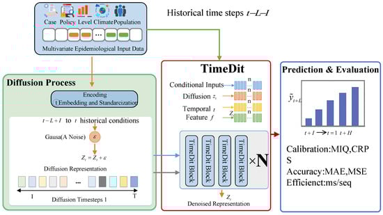
Figure 2. CNL-Diff architecture.

2.1. Diffusion Model

Diffusion models are a class of generative modeling frameworks based on latent variables. Given a data sample ($x\sim q\left(x\right)$), the forward noise process gradually generates a sequence of latent variables ($x^0,x^1,x^2,\dots ,x^T$), while the reverse process generates these latent variables in reverse order to reconstruct the original data (x).

In standard diffusion models, the forward process is modeled as a linear Gaussian Markov chain [10,51]. For example, in the Denoising Diffusion Probabilistic Model (DDPM), at the t-th step, the latent variable ($x^t$) is generated by multiplying the previous state ($x^{t-1}$) by a coefficient ($\sqrt{{\alpha }_t}$) and adding Gaussian noise with mean zero and variance $(1-{\alpha }_t)$, which is expressed as the conditional distribution:

$$q\left(x^t\right|x^{t-1})=\mathcal{N}(x^t;\sqrt{{\alpha }_t}{x}^{t-1},(1-{\alpha }_t)I)$$

The reverse process is modeled by a Markov chain of the following form:

$$p_{\theta }\left(x_{0:T}\right)=p\left(x_T\right)\prod _{t=1}^T{p}_{\theta }\left(x_{t-1}\right|x_t)$$

where the prior distribution is set as $p\left(x_T\right)=\mathcal{N}(x_T;0,I)$. The combination of the forward process and the parameterized reverse process ($p_{\theta }$) forms a structure similar to a hierarchical variational autoencoder [52]. During training, the model optimizes the parameters by minimizing the variational lower bound on the negative log likelihood, with the objective function expressed as follows:

$$L={\mathbb{E}}_q\left[D_{\mathrm{KL}}\left(q\left(x_T\right|x)\parallel p\left(x_T\right)\right)-log{p}_{\theta }\left(x\right|x_0)+\sum _{t=1}^T{D}_{\mathrm{KL}}\left(q\left(x_{t-1}\right|x_t,x)\parallel p_{\theta }\left(x_{t-1}\right|x_t)\right)\right]$$

To estimate the noise or the original data, two approaches can be used: noise prediction or data prediction. If the data prediction method is used, the denoising network (${ϵ}_{\theta }$) is employed to recover $x_0$ from the noisy latent variable ($x_t$), and the model is trained by minimizing the following loss function:

$$L_{ϵ}={\mathbb{E}}_q\left[\parallel ϵ-{ϵ}_{\theta }(x_t,t){\parallel }^2\right]$$

In the context of time-series modeling, previous studies have shown that directly predicting the original data ($x_0$) is usually more effective than predicting the noise ($ϵ$) [20,53]. Based on this conclusion, this paper adopts the data prediction modeling strategy in the implementation.

2.2. Conditional Diffusion Models

In time-series forecasting tasks, the goal is to predict future values ($x_{L+1:T}\in {\mathbb{R}}^{d\times H}$) based on the historical observation sequence ($x_{-L+1:T}\in {\mathbb{R}}^{d\times L}$, where L represents the lookback window length, H is the prediction window length, and d is the dimensionality of the variables; superscripts and subscripts denote the time step of the diffusion process and the time step of the sequence, respectively). When using conditional diffusion models for time-series forecasting, the following conditional distribution is considered:

$$p_{\theta }(x^0:T|x_{1:T}\left|c\right)=p_{\theta }\left(x_T\right|c)\prod _{t=1}^T{p}_{\theta }\left(x_{t-1}\right|x_t,c)$$

where $x_T\sim \mathcal{N}(0,I)$ and the specific form of the conditional variable (c) varies across different models [17,19,20,21]. The denoising process at each time step is defined as follows:

$$p_{\theta }\left(x_{t-1}\right|x_t,x_{1:T},c)=\mathcal{N}(x_{t-1};{\mu }_{\theta }(x_t,t|c),{\sigma }_t^{2}I)$$

During the inference phase, generated samples are associated with the initial noise vector (${\widehat{x}}_T$), which is sampled from the standard Gaussian distribution ($\mathcal{N}(0,I)$). The denoising step is iteratively applied until the time step is $t=1$, ultimately producing the predicted sequence (${\widehat{x}}_{1:H}$).

Explicitly introducing the conditional variable (c) as the terminal prior mean of the forward diffusion process can be viewed as a natural extension of classical diffusion models in which the isotropic Gaussian prior is replaced by a condition-dependent Gaussian distribution, thereby ensuring probabilistic consistency between forward and reverse conditioning [10,51]. Compared to injecting conditioning only into the reverse denoiser, embedding c directly into the forward marginal provides a global anchor over the entire diffusion time horizon, which is consistent with empirical findings in conditional and guided diffusion models and improves the stability and controllability of conditional generation [11,54,55]. In practice, this design mitigates multi-modal uncertainty and leads to more stable training dynamics, as well as improved predictive calibration, particularly for structured prediction and time-series forecasting tasks.

While Transformers and diffusion models have been explored for generic time-series forecasting, CNL-Diff differs from prior studies in two essential aspects. First, instead of adopting a fixed linear–Gaussian forward process and introducing conditions only during reverse denoising, we incorporate a forward–backward consistent conditioning mechanism by learning a condition-dependent prior and embedding conditional guidance directly into the forward diffusion formulation. Second, we introduce a learnable nonlinear, time-dependent data transformation within the diffusion forward marginal, explicitly targeting the nonlinearity, non-stationarity, and multi-modal/heavy-tailed behaviors commonly observed in epidemic scale trajectories. Together, these designs make CNL-Diff particularly suitable for epidemic scale forecasting and early warning under distribution shifts and irregular outbreaks.The structural differences between CNL-Diff, DDPM, and conditional DDPM are shown in Figure 3.

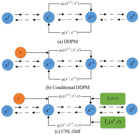
Figure 3. Structural comparison of CNL-Diff, DDPM, and conditional DDPM.

2.3. Formulation

In this section, we present the formal representation of CNL-Diff, with the specific structure shown in Figure 4

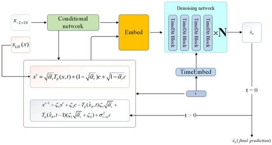
Figure 4. Structure of CNL-Diff with formulas.

We define the nonlinear, time-dependent data transformation as the following marginal distribution:

$$q_{\varphi }(x_{1:H}^t\mid x_{1:H})=\mathcal{N}\left(x_{1:H}^t;\sqrt{{\overline{\alpha }}_t}{T}_{\varphi }(x_{1:H},t),(1-{\overline{\alpha }}_t)I\right),$$

where

$$T_{\varphi }(x_{1:H},t):{\mathbb{R}}^{d\times H}\times [0,T]\to {\mathbb{R}}^{d\times H}$$

is a nonlinear neural operator controlled by the $\varphi$ parameter, which applies a time-dependent transformation to the input data ($x_{1:H}$). To simplify notation, we refer to $x_{1:H}$ as x.

Furthermore, we introduce a learnable conditional variable (c) in the forward process, inspired by image diffusion models. At this point, the marginal distribution can be expressed as follows (the structural diagram is shown in Figure 4):

$$q_{\varphi }(x^t\mid x,c)=\mathcal{N}\left(x^t;\sqrt{{\overline{\alpha }}_t}{T}_{\varphi }(x,t)+(1-\sqrt{{\overline{\alpha }}_t})c,(1-{\overline{\alpha }}_t)I\right).$$

Equation (1) defines a Gaussian forward marginal whose mean is an affine (mean-shift) interpolation between the transformed data ($T_{\varphi }(x,t)$) and a learnable conditional anchor (c). This design is chosen for two reasons. First, it preserves the Gaussian Markov structure and keeps $q_{\varphi }(x^t\mid x,c)$ analytically tractable, thereby enabling standard diffusion training with a closed-form posterior. Second, the coefficient ($\sqrt{{\overline{\alpha }}_t}$) enforces intuitive boundary behaviors: when $t\to 0$ ($\sqrt{{\overline{\alpha }}_t}\to 1$), the mean approaches $T_{\varphi }(x,0)$, keeping $x^t$ close to the data manifold; when $t\to T$ ($\sqrt{{\overline{\alpha }}_t}\to 0$), the mean approaches c, and the marginal becomes approximately $\mathcal{N}(c,I)$, yielding a condition-dependent terminal distribution.

Classical diffusion assumes that gradually adding linear Gaussian noise provides a convenient path from data to an isotropic Gaussian prior. However, epidemic incidence trajectories often exhibit heavy tails, heteroscedastic variance, and multi-modal peaks, making the “data-to-Gaussian” path highly distorted. We introduce a learnable, time-dependent transform ($T_{\varphi }(·,t)$) to partially “re-shape” the data manifold before noise accumulation, aiming to reduce distribution mismatch and simplify reverse denoising. Conceptually, $T_{\varphi }$ plays a role analogous to a lightweight learned re-parameterization (or partial Gaussianization) that makes the diffusion trajectory more consistent with a Gaussian terminal distribution conditioned on c.

The introduced nonlinear transformation ($T_{\varphi }(x,t)$) does not disrupt the temporal structure of the data, as it operates under strict structural constraints that preserve the original time ordering and sequence dimensionality. Specifically, $T_{\varphi }$ acts on the entire time-series representation, without any permutation or mixing of temporal indices, ensuring that temporal continuity is maintained. Moreover, the nonlinear transformation is incorporated into the forward diffusion process in a progressive, difference-based manner across diffusion time steps rather than as a direct replacement of the original sequence. This design allows nonlinear information to be injected smoothly along the diffusion trajectory, while the inherent temporal dependencies are still governed by the gradual noising mechanism of diffusion. As a result, the model can adaptively reshape the data representation to better capture temporal dynamics and correlations, without compromising the underlying time structure of the sequence.

When $t=T$ and the noise schedule parameters (${\alpha }_t,{\overline{\alpha }}_T$) are adjusted to approach 0, we obtain the following:

$$q_{\varphi }(x^T\mid x,c)\approx \mathcal{N}(c,I).$$

This implies that $\mathcal{N}(c,I)$ forms a learnable prior distribution, and during inference, the reverse generation process must be executed based on this prior.

2.4. Denoising Network

TimeDiT [18] is an innovative method that integrates diffusion models with the Transformer architecture. It can effectively capture complex dependencies and nonlinear features in the time-series data of infectious disease scale and incorporate external condition information such as seasonal changes and policy interventions into the time-series forecasting process. This method uses a Transformer-based structure to process multivariate time-series data. We employ the TimeDiT module, the specific architecture of which is shown in Figure 5. In the model, the noisy target sequence embedding $x_t^{\mathrm{tar}}$ (with noise schedule ${\beta }_t\in (0,1)$) and the conditional observation ($x_0^{\mathrm{con}}$) are jointly input into the TimeDiT module, where a multi-head attention mechanism is used to learn the complex dependencies in the data.

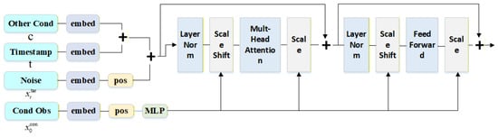
Figure 5. Structure of the TimeDiT block (enlarged for improved readability).

In the design of the diffusion process, TimeDiT differs from previous methods [56,57] by directly injecting the diffusion time-step information into the target noise vector, leveraging this information to maintain global consistency across the entire noisy sequence.

For the integration of conditional information, traditional approaches typically concatenate the conditional vector with the input sequence directly [58]. In contrast, TimeDiT adopts the Adaptive Layer Normalization (AdaLN) method, using partial observations ($x_0^{\mathrm{con}}$) to control the scale and shift of the target sequence ($x_0^{\mathrm{tar}}$):

$$\mathrm{AdaLN}(h,c)=c_{\mathrm{scale}}\mathrm{LayerNorm}\left(h\right)+c_{\mathrm{shift}},$$

where h is the hidden state and $c_{\mathrm{scale}}$ and $c_{\mathrm{shift}}$ are scale and shift parameters derived from $x_0^{\mathrm{con}}$, respectively. This method is more effective than direct concatenation, as it fully utilizes the scale and shift features contained in $x_0^{\mathrm{con}}$, which is crucial for capturing temporal continuity and dynamic evolution.

3. Results

3.1. Dataset and Preprocessing

To comprehensively evaluate the proposed CNL-Diff framework, we conduct experiments on the officially published monthly and weekly statutory infectious disease surveillance data from the Chinese Center for Disease Control and Prevention (China CDC). The dataset covers 31 province-level administrative regions (excluding Hong Kong, Macao, and Taiwan) and spans from January 2010 to December 2024, including 37 notifiable infectious diseases across Classes A, B, and C. In total, the corpus contains more than 1.8 million multivariate spatiotemporal records, encompassing epidemiological, demographic, climatic, and policy-related attributes.

Although the surveillance records are obtained from a single national reporting system (China CDC), the dataset is inherently multi-disease and multi-condition: it covers 37 notifiable infectious diseases across Classes A/B/C, 31 province-level regions, and both weekly and monthly reporting schedules from 2010 to 2024. Therefore, our evaluation is not limited to a single disease scenario; instead, it spans heterogeneous epidemic dynamics (seasonal recurrent diseases, sporadic outbreak-prone diseases, and diverse regional patterns). Consistent with this design, our study focuses on the general idea of epidemic-scale forecasting and early warning across infectious diseases rather than optimizing for one specific pathogen.

To assess the robustness of CNL-Diff across diseases with diverse epidemiological characteristics, we select eight representative diseases exhibiting strong heterogeneity in seasonality, volatility, and outbreak patterns: hand–foot–mouth disease (HFMD), influenza, tuberculosis, viral hepatitis, scarlet fever, dengue fever, mumps, and bacillary dysentery. This selection covers both strongly seasonal diseases (e.g., influenza and HFMD) and sporadic outbreak-prone diseases (e.g., dengue), providing a stringent testbed for probabilistic forecasting models.

Notably, while several diseases exhibit recurrent seasonal peaks, their peak timing and magnitude can shift across years and regions due to climate variability, interventions, population mobility, and reporting practices. Therefore, our forecasting objective is not merely to reproduce a fixed cycle but to provide accurate and well-calibrated probabilistic predictions of both peak timing and epidemic scale.

All data undergo the unified preprocessing strategy shown in Table 1. Linear interpolation is used as a simple within-series imputation strategy to maintain temporal continuity when sporadic missing entries occur. Zero padding is applied only for sequence-length alignment during batching and should not be interpreted as genuine zero incidence for missing observations. We acknowledge that interpolation and padding may smooth abrupt outbreak peaks or introduce artificial near-zero segments when missingness concentrates around peak periods. Alternative strategies include mask-aware modeling, spline or Kalman smoothing, and diffusion-based imputation; we leave the systematic evaluation of these alternatives to future work. We apply a transformation expressed $y=log(1+x)$ to mitigate extreme peaks and heavy-tailed behavior. The inverse transform is given by $x=exp\left(y\right)-1$. Unless otherwise stated, we report final forecast values and interpret results in the original scale after applying the inverse transformation.

Table 1. Dataset column names and processing methods.

Column Name	Meaning	Processing Method
time	Time	Convert to continuous time index (t = 1, 2, …, T)
disease name	Disease name	One-hot encoding
region	Regional jurisdiction	One-hot encoding
cases	Number of cases	$log(1+x)$
deaths	Number of deaths	Same as above; can also be added as a feature
population	Population of region	Used for normalization and calculation of the disease rate
policy level	Policy level	One-hot encoding
climate temp	Average temperature	Normalize and add condition features

Missing values are imputed using linear interpolation, and all sequences are padded with zeros for consistent temporal alignment. Incidence-rate series are further transformed using

$$log(1+x)$$

to mitigate extreme peaks and heavy-tailed behavior.

The dataset is divided chronologically (to avoid information leakage):

• Training: 2010–2019;
• Validation: 2020–2021;
• Testing: 2022–2024.

In total, we obtain approximately 42,000 training sequences, each with a minimum temporal length of ≥120 time steps.

3.2. Implementation Details

The model is implemented using PyTorch 2.3, with the backbone denoising network being TimeDiT-Base (approximately 86M parameters). The look-back window is $L\in \{24,48,72,120\}$ (with the main experiment using a weekly look-back), and the forecast horizon is $H\in \{1,3,6,12\}$. The number of diffusion steps during training is $T=100$, and during inference, DDIM is used for acceleration to 20 steps, with a cosine noise schedule. The AdamW is the used optimizer (lr = 1 × 10⁻⁴, weight_decay = 0.01), with a batch size of 128. Training is performed on 4 × A100 (40 GB) for approximately 36 h to converge. We report the average metrics for $H=1,3,6,12$, with all experiments repeated five times to determine the mean.

To facilitate reproduction of the comparison in Table 2, we summarize the configurations of key baselines. For ARIMA/SARIMA, each disease–region series is fitted using standard statistical toolkits; model orders are selected on the training split by minimizing information criteria (e.g., AIC), and seasonal periods are set according to the reporting frequency (e.g., $m=12$ for monthly data and $m=52$ for weekly data when seasonality is modeled). Multi-step forecasts for horizons of $H\in \{1,3,6,12\}$ are generated iteratively. Prophet is trained with its standard additive components and seasonality settings aligned with the data frequency. Deep learning baselines (LSTM/TCN/Informer/FEDformer) follow the same lookback–horizon protocol and are tuned on the validation set. Diffusion-based baselines (CSDI/D3VAE/DiffWave) are implemented following their original papers, with sampling settings adapted to our horizons. Importantly, all baselines share the same preprocessing and chronological splits described in the Section 3.1 to avoid information leakage.

Table 2. Comparison of models.

Model	MAE	MSE	CRPS	PICP (%)	MPIW	Inference Time (ms)
ARIMA	15.32 ± 0.46	222.1 ± 11.5	9.58 ± 0.41	80.1	50.4	62
SARIMA	14.69 ± 0.43	208.7 ± 10.3	9.18 ± 0.37	82.6	48.0	65
Prophet	13.44 ± 0.41	193.9 ± 9.6	8.36 ± 0.35	85.0	45.3	54
SEIR	16.05 ± 0.49	233.2 ± 11.8	10.04 ± 0.44	79.2	52.0	70
LSTM	11.28 ± 0.36	162.1 ± 8.4	6.88 ± 0.31	87.1	40.5	136
TCN	10.74 ± 0.34	153.9 ± 7.7	6.47 ± 0.28	88.5	38.7	122
Informer	10.35 ± 0.33	148.8 ± 7.4	6.17 ± 0.27	89.9	37.2	164
FEDformer	9.96 ± 0.31	143.7 ± 7.1	5.86 ± 0.26	90.8	36.2	156
TimesNet	10.58 ± 0.33	151.2 ± 7.6	6.35 ± 0.27	88.9	38.0	148
PatchTST	9.88 ± 0.31	142.9 ± 7.0	5.82 ± 0.26	91.0	36.0	158
iTransformer	9.72 ± 0.30	140.6 ± 6.9	5.69 ± 0.25	91.4	35.6	162
Chronos	8.34 ± 0.26	114.2 ± 5.9	4.52 ± 0.21	94.0	31.4	185
DiffWave	8.55 ± 0.27	118.6 ± 6.1	4.68 ± 0.22	93.5	32.1	207
D3VAE	8.97 ± 0.28	126.4 ± 6.6	5.05 ± 0.23	92.2	33.3	196
CSDI	9.14 ± 0.29	128.9 ± 6.6	5.27 ± 0.24	92.1	34.0	213
CNL-Diff (Ours)	7.76 ± 0.26	103.9 ± 5.7	3.96 ± 0.20	95.0	29.2	233

3.3. Evaluation Metrics

To evaluate deterministic accuracy, probabilistic calibration, and computational efficiency, we use the following metrics:

• Deterministic metrics:

  $$\mathrm{MAE}={\displaystyle \frac{1}{N}}\sum _{i=1}^N\left|{\widehat{y}}_i-y_i\right|,\mathrm{MSE}={\displaystyle \frac{1}{N}}\sum _{i=1}^N{({\widehat{y}}_i-y_i)}^2$$

  where ${\widehat{y}}_i$ is the predicted value and $y_i$ is the ground truth.
• Probabilistic metrics:

  $$\mathrm{CRPS}={\int }_{-\infty }^{\infty }\left|F_{\widehat{y}}\left(x\right)-F_y\left(x\right)\right|dx$$

  where $F_{\widehat{y}}\left(x\right)$ is the cumulative distribution function (CDF) of the prediction and $F_y\left(x\right)$ is the CDF of the ground truth.

  $$\mathrm{PICP}={\displaystyle \frac{1}{N}}\sum _{i=1}^N\mathbb{I}\left({\widehat{y}}_{\alpha ,i}\le y_i\le {\widehat{y}}_{1-\alpha ,i}\right)$$

  where $\mathbb{I}(·)$ is the indicator function; ${\widehat{y}}_{\alpha ,i}$ and ${\widehat{y}}_{1-\alpha ,i}$ represent the lower and upper bounds of the prediction interval, respectively; and $\alpha =0.05$ for a 90% prediction interval.

  $$\mathrm{MPIW}={\displaystyle \frac{1}{N}}\sum _{i=1}^N({\widehat{y}}_{1-\alpha ,i}-{\widehat{y}}_{\alpha ,i})$$

  where ${\widehat{y}}_{\alpha ,i}$ and ${\widehat{y}}_{1-\alpha ,i}$ are the lower and upper bounds of the prediction interval for the i-th sample, respectively.

To quantify sampling uncertainty, we report results as mean ± standard deviation across repeated runs and additionally provide 95% confidence intervals via bootstrap over province–disease series.

3.4. Comparison with Mainstream Methods

We perform a comprehensive comparison of CNL-Diff with four categories of representative baselines:

• Traditional Statistical/Dynamical Models: ARIMA, SARIMA, Prophet [59], and SEIR;
• Deep Sequence Models: LSTM, TCN [60], Informer [45], FEDformer [46], TimesNet [61], iTransformer [62], and Chronos [63];
• Generative Probabilistic Forecasting Models: CSDI [16], D3VAE [64], and DiffWave [65].

Figure 6 provides qualitative forecasting trajectories by selecting one representative best-performing method from each major baseline category in Table 2: Prophet (statistical forecasting), Informer (Transformer-based forecasting), and CSDI (diffusion-based probabilistic forecasting), together with our CNL-Diff. We observe that CNL-Diff is particularly advantageous for (i) strongly seasonal diseases, where distributional forecasts benefit from conditioning on exogenous drivers, and (ii) outbreak-prone diseases with abrupt peaks, where purely linear–Gaussian diffusion assumptions may underfit tail behavior. This is consistent with our heterogeneous disease set, which includes both highly seasonal and sporadic outbreak-prone diseases. We also note potential failure modes: if reporting delays or missingness are concentrated around peak periods, simple interpolation or padding can smooth peak dynamics and may bias peak magnitude or timing. This motivates future work on mask-aware and more robust imputation schemes.

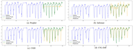
Figure 6. Visualizations of dataset predictions by (a) Prophet [59], (b) Informer [45], (c) CSDI [16], and (d) CNL-Diff.

As shown in Table 2, CNL-Diff achieves the best average performance across all key metrics, including MAE, MSE, CRPS, PICP, and MPIW, while exhibiting relatively small variance across repeated runs. In particular, the model demonstrates strong probabilistic calibration by maintaining high coverage with narrower prediction intervals. Compared with the strongest traditional baseline, i.e., Prophet, CNL-Diff reduces the average MAE, MSE, and CRPS by approximately 42–48%, with the improvements being consistently supported by the reported confidence intervals. Relative to the best-performing deep sequence model, i.e., FEDformer, CNL-Diff shows an average improvement of around 22% across metrics and maintains stable advantages across runs. Against generative baselines, CNL-Diff improves CRPS by about 15%, increases PICP by 1.6%, and reduces MPIW by 8.9% compared to DiffWave. Moreover, even when compared with recent diffusion-based models proposed in 2025, CNL-Diff retains a 10–25% average advantage in CRPS. In medium- and long-term forecasting (H = 12), CNL-Diff further reduces the MAE by approximately 18–22%, indicating robust performance under complex temporal disturbances.

3.5. Comparison Using Different Denoising Networks

To identify an appropriate denoising network, we compared several candidate architectures, and the results are summarized in Table 3. Overall, TimeDiT achieves the best average performance across multiple evaluation metrics. In terms of point forecasting accuracy, TimeDiT attains the lowest MAE (7.81) and MSE (105.3), outperforming the next best model by approximately 10.3% and 11.1%, respectively, with the advantages being consistently supported across repeated runs.

Table 3. Comparison with diffusion-based baselines.

Model	MAE	MSE	CRPS	PICP (%)	MPIW	Inference Time (ms)
TimeDiT	$7.76\pm 0.26$	$103.9\pm 5.7$	$3.96\pm 0.20$	95.0	29.2	233
Diffolio [66]	$8.66\pm 0.28$	$117.9\pm 6.0$	$4.69\pm 0.22$	91.2	32.8	194
EPDiff [67]	$9.58\pm 0.30$	$131.1\pm 6.9$	$5.27\pm 0.24$	88.3	35.1	108
WIDT [68]	$9.08\pm 0.29$	$122.9\pm 6.4$	$4.95\pm 0.23$	90.4	34.0	180
MSDT [69]	$9.27\pm 0.29$	$127.4\pm 6.7$	$4.48\pm 0.22$	91.2	32.3	156
TAD [70]	$8.98\pm 0.28$	$124.6\pm 6.3$	$4.24\pm 0.21$	91.3	33.7	145

TimeDiT also demonstrates strong probabilistic prediction performance, achieving the lowest CRPS (4.01), the highest PICP (94.8%), and the narrowest MPIW (29.5), indicating a favorable balance between predictive accuracy, uncertainty calibration, and interval sharpness. Among the baselines, TAD performs relatively well on CRPS, while MSDT shows comparatively compact prediction intervals; however, neither matches TimeDiT in overall performance consistency.

Although EPDiff exhibits superior inference efficiency (108 ms), its prediction accuracy is notably lower across all metrics, highlighting the trade-off between efficiency and predictive performance. In contrast, TimeDiT maintains the best overall forecasting performance while keeping its inference time (230 ms) within an acceptable range. Therefore, considering both performance robustness and computational cost, we select TimeDiT as the denoising network.

3.6. Ablation Study

To elucidate the contributions of key components within CNL-Diff, we perform extensive ablation studies focusing on the following:

• Full Model: Forward–backward consistent conditioning + nonlinear transform + TimeDiT denoiser;
• Diff: Standard unconditional DDPM (no conditioning (c) and no nonlinear transform);
• Cond Diff: Conditional diffusion where conditioning is injected only in the reverse denoiser, while the forward process remains a fixed linear–Gaussian path;
• w/o $T_{\varphi }$: Remove nonlinear forward transform (set $T_{\varphi }$ to identity);
• Feature Dim: The nonlinear transformation is applied only along the feature (variable) dimension.
• Forecast Window: The nonlinear transformation is applied only along the temporal dimension corresponding to the forecast window.
• U-Net: Replace TimeDiT with a U-Net-style denoiser while keeping other components unchanged.

The ablation results reported in Table 4 demonstrate the contribution of each model component to overall performance and uncertainty quantification. Removing the forward–backward consistent conditioning mechanism (w/o Cond) leads to a noticeable degradation in average probabilistic forecasting performance, accompanied by increased variability across runs, indicating that explicitly modeling external driving factors—such as policy interventions, climate conditions, and regional heterogeneity—during the noise injection phase is critical for reliable uncertainty estimation. Introducing conditional information only in the reverse process still results in an average MAE increase of approximately 9%, suggesting that the forward conditional prior plays an important role in maintaining generation consistency.

Table 4. Ablation study.

Description	MAE	MSE	CRPS	PICP (%)	MPIW
Full Model	$7.76\pm 0.26$	$103.9\pm 5.7$	$3.96\pm 0.20$	95.0	29.2
Diff	$8.97\pm 0.28$	$121.0\pm 6.2$	$4.84\pm 0.22$	90.2	33.2
Cond Diff	$8.49\pm 0.27$	$114.6\pm 6.0$	$4.65\pm 0.21$	91.5	32.1
Without $T_{\varphi }$	$9.36\pm 0.29$	$126.2\pm 6.6$	$5.06\pm 0.24$	89.7	34.5
Feature Dim	$8.29\pm 0.27$	$110.9\pm 5.8$	$4.35\pm 0.21$	93.4	30.8
Forecast Window	$8.46\pm 0.27$	$111.6\pm 5.9$	$4.55\pm 0.21$	92.1	31.5
U-Net	$9.08\pm 0.29$	$123.1\pm 6.3$	$4.95\pm 0.23$	90.5	33.8

Completely removing the nonlinear transformation unit ($T_{\psi }$) causes severe performance degradation, with the average CRPS deteriorating by more than 35%, and this trend remains consistent across repeated experiments. This observation reflects the limitations of traditional linear Gaussian assumptions when modeling the complex dynamics of real-world epidemics. Further ablation results indicate that applying nonlinear transformations along only a single dimension (either temporal or feature-wise) can partially alleviate the performance loss, whereas a cooperative transformation across both dimensions is required to effectively capture the time–feature joint distribution distortion induced by abrupt peak events.

4. Discussion

4.1. Main Findings

Across large-scale statutory infectious disease surveillance data, the proposed CNL-Diff framework consistently improves both point-forecast accuracy and probabilistic calibration. The ablation study (Table 4) further indicates that (i) forward–backward consistent conditioning is important for stable uncertainty quantification and (ii) the nonlinear transformation unit ($T_{\psi }$) substantially reduces distributional distortion, thereby easing the reverse denoising task and improving CRPS and interval quality.

4.2. Practical Applications for Public Health Decision Making

The primary goal of epidemic scale forecasting is to support actionable public health decisions rather than to optimize statistical metrics alone. In practice, probabilistic forecasts generated by CNL-Diff can be used in at least three ways:

• Early warning via risk thresholds: Given generated samples (${\left\{{\widehat{y}}_{t+h}^{\left(s\right)}\right\}}_{s=1}^S$), practitioners can compute the probability of exceeding an alert threshold ($\tau$) as $\mathbb{P}({\widehat{y}}_{t+h}>\tau )\approx {\displaystyle \frac{1}{S}}{\sum }_{s=1}^S\mathbb{I}({\widehat{y}}_{t+h}^{\left(s\right)}>\tau )$, enabling risk-based alarms.
• Peak timing and magnitude planning: The predictive distribution supports uncertainty-aware estimation of peak week and peak magnitude (e.g., quantiles of peak timing), which can inform hospital bed allocation, drug and vaccine logistics, and staffing.
• Uncertainty-aware communication: Calibrated intervals (PICP/MPIW) allow decision makers to communicate forecast confidence and avoid over-reliance on single deterministic trajectories.

4.3. Seasonality and Interpretation Under Regular Peak Cycles

Many infectious diseases exhibit recurrent seasonal patterns, so peak cycles may appear regular at an annual scale. However, seasonality does not eliminate the need for forecasting. Public health decisions depend on when the peak arrives (phase shifts), how large it becomes (severity), and how uncertain the outlook is (calibration), all of which can vary substantially across years and regions. In this setting, CNL-Diff is designed to model both the dominant seasonal component and the complex residual dynamics driven by exogenous factors (e.g., interventions, climate anomalies, and population mobility), providing probabilistic forecasts that remain informative, even when the baseline cycle is stable.

4.4. Discrepancies Between Predicted and Observed Values

We observed that prediction errors are more pronounced around abrupt regime changes and rare extreme peaks, where the data distribution may shift relative to the training period. Several factors may contribute to the remaining discrepancies:

• Distribution shift and interventions: Policy changes, behavioral responses, and emergent variants can rapidly alter transmission dynamics, leading to shifts that are difficult to infer from historical patterns alone.
• Reporting delay and measurement noise: Surveillance data may contain backfilling, under-reporting, and heterogeneous reporting practices across regions and diseases, which can blur peak shapes.
• Unmodeled covariates: Variables such as school calendars, mobility, and extreme weather can modulate transmission but may not be fully captured by the available conditioning features.
• Rare-event sparsity: Extreme outbreaks are low-frequency events; diffusion sampling may smooth rare spikes unless specialized loss weighting or peak-aware objectives are introduced.

These observations motivate future work on the integration of richer exogenous features, peak-aware training objectives, and domain adaptation strategies to better handle regime shifts.

References

- Chen, Y.; Zhang, C.; Ma, M.; Liu, Y.; Ding, R.; Li, B.; He, S.; Rajmohan, S.; Lin, Q.; Zhang, D. Imdiffusion: Imputed diffusion models for multivariate time series anomaly detection. arXiv 2023, arXiv:2307.00754. [Google Scholar] [CrossRef]
- Nguyen, H.D.; Tran, K.P.; Thomassey, S.; Hamad, M. Forecasting and Anomaly Detection approaches using LSTM and LSTM Autoencoder techniques with the applications in supply chain management. Int. J. Inf. Manag. 2021, 57, 102. [Google Scholar] [CrossRef]
- Xia, X.; Pan, X.; Li, N.; He, X.; Ma, L.; Zhang, X.; Ding, N. GAN-based anomaly detection: A review. Neurocomputing 2022, 493, 497–535. [Google Scholar] [CrossRef]
- Pang, G.; Shen, C.; Cao, L.; Hengel, A.V.D. Deep learning for anomaly detection: A review. ACM Comput. Surv. (CSUR) 2021, 54, 38. [Google Scholar] [CrossRef]
- Choi, K.; Yi, J.; Park, C.; Yoon, S. Deep learning for anomaly detection in time-series data: Review, analysis, and guidelines. IEEE Access 2021, 9, 120043–120065. [Google Scholar] [CrossRef]
- Garg, A.; Zhang, W.; Samaran, J.; Savitha, R.; Foo, C.S. An evaluation of anomaly detection and diagnosis in multivariate time series. IEEE Trans. Neural Netw. Learn. Syst. 2021, 33, 2508–2517. [Google Scholar] [CrossRef]
- Schmidl, S.; Wenig, P.; Papenbrock, T. Anomaly detection in time series: A comprehensive evaluation. Proc. VLDB Endow. 2022, 15, 1779–1797. [Google Scholar] [CrossRef]
- Wu, R.; Keogh, E.J. Current time series anomaly detection benchmarks are flawed and are creating the illusion of progress. IEEE Trans. Knowl. Data Eng. 2021, 35, 2421–2429. [Google Scholar] [CrossRef]
- Liu, Y.; Luo, T.; Zhao, P.; Wang, J.; Cao, Z. Early Warning Methods Based on a Real Time Series Dataset: A Comparative Study. In Proceedings of the China National Conference on Big Data and Social Computing, Harbin, China, 8–10 August 2024; Springer: Singapore, 2024; pp. 3–18. [Google Scholar] [CrossRef]
- Ho, J.; Jain, A.; Abbeel, P. Denoising diffusion probabilistic models. Adv. Neural Inf. Process. Syst. 2020, 33, 6840–6851. [Google Scholar]
- Dhariwal, P.; Nichol, A. Diffusion models beat gans on image synthesis. Adv. Neural Inf. Process. Syst. 2021, 34, 8780–8794. [Google Scholar]
- Harvey, W.; Naderiparizi, S.; Masrani, V.; Weilbach, C.; Wood, F. Flexible diffusion modeling of long videos. Adv. Neural Inf. Process. Syst. 2022, 35, 27953–27965. [Google Scholar]
- Blattmann, A.; Rombach, R.; Ling, H.; Dockhorn, T.; Kim, S.W.; Fidler, S.; Kreis, K. Align your latents: High-resolution video synthesis with latent diffusion models. In Proceedings of the IEEE/CVF Conference on Computer Vision and Pattern Recognition, Vancouver, BC, Canada, 17–24 June 2023; pp. 22563–22575. [Google Scholar]
- Mothish, G.; Tayal, M.; Kolathaya, S. Birodiff: Diffusion policies for bipedal robot locomotion on unseen terrains. In Proceedings of the 2024 Tenth Indian Control Conference (ICC), Bhopal, India, 9–11 December 2024; pp. 385–390. [Google Scholar] [CrossRef]
- Saharia, C.; Chan, W.; Saxena, S.; Li, L.; Whang, J.; Denton, E.L.; Ghasemipour, K.; Gontijo Lopes, R.; Karagol Ayan, B.; Salimans, T. Photorealistic text-to-image diffusion models with deep language understanding. Adv. Neural Inf. Process. Syst. 2022, 35, 36479–36494. [Google Scholar]
- Tashiro, Y.; Song, J.; Song, Y.; Ermon, S. Csdi: Conditional score-based diffusion models for probabilistic time series imputation. Adv. Neural Inf. Process. Syst. 2021, 34, 24804–24816. [Google Scholar]
- Li, Y.; Chen, W.; Hu, X.; Chen, B.; Sun, B.; Zhou, M. Transformer-modulated diffusion models for probabilistic multivariate time series forecasting. In Proceedings of the Twelfth International Conference on Learning Representations, Vienna, Austria, 7–11 May 2024. [Google Scholar]
- Cao, D.; Ye, W.; Zhang, Y.; Liu, Y. Timedit: General-purpose diffusion transformers for time series foundation model. arXiv 2024, arXiv:2409.02322. [Google Scholar]
- Shen, L.; Chen, W.; Kwok, J. Multi-resolution diffusion models for time series forecasting. In Proceedings of the The Twelfth International Conference on Learning Representations, Vienna, Austria, 7–11 May 2024. [Google Scholar]
- Shen, L.; Kwok, J. Non-autoregressive conditional diffusion models for time series prediction. In Proceedings of the International Conference on Machine Learning, Honolulu, HI, USA, 23–29 July 2023; pp. 31016–31029. [Google Scholar]
- Rasul, K.; Seward, C.; Schuster, I.; Vollgraf, R. Autoregressive denoising diffusion models for multivariate probabilistic time series forecasting. In Proceedings of the International Conference on Machine Learning, Virtual, 18–24 July 2021; pp. 8857–8868. [Google Scholar]
- Malhotra, P.; Vig, L.; Shroff, G.; Agarwal, P. Long short term memory networks for anomaly detection in time series. In Proceedings of the European Symposium on Artificial Neural Networks, Computational Intelligence, and Machine Learning, Bruges, Belgium, 22–24 April 2015; Volume 89, p. 94. [Google Scholar]
- Wang, Y.; Li, J. Anomaly detection method for time series data based on transformer reconstruction. In Proceedings of the 2023 12th International Conference on Informatics, Environment, Energy and Applications, Singapore, 17–19 February 2023; pp. 58–63. [Google Scholar] [CrossRef]
- Guo, Z.; He, K.; Xiao, D. Early warning of some notifiable infectious diseases in China by the artificial neural network. R. Soc. Open Sci. 2020, 7, 191420. [Google Scholar] [CrossRef] [PubMed]
- Park, D.; Hoshi, Y.; Kemp, C.C. A multimodal anomaly detector for robot-assisted feeding using an lstm-based variational autoencoder. IEEE Robot. Autom. Lett. 2018, 3, 1544–1551. [Google Scholar] [CrossRef]
- Zhang, Y.; Chen, Y.; Wang, J.; Pan, Z. Unsupervised deep anomaly detection for multi-sensor time-series signals. IEEE Trans. Knowl. Data Eng. 2021, 35, 2118–2132. [Google Scholar] [CrossRef]
- Akcay, S.; Atapour-Abarghouei, A.; Breckon, T.P. Ganomaly: Semi-supervised anomaly detection via adversarial training. In Proceedings of the Asian Conference on Computer Vision, Perth, Australia, 2–6 December 2018; Springer: Cham, Switzerland, 2018; pp. 622–637. [Google Scholar] [CrossRef]
- Du, B.; Sun, X.; Ye, J.; Cheng, K.; Wang, J.; Sun, L. GAN-based anomaly detection for multivariate time series using polluted training set. IEEE Trans. Knowl. Data Eng. 2021, 35, 12208–12219. [Google Scholar] [CrossRef]
- Qi, L.; Yang, Y.; Zhou, X.; Rafique, W.; Ma, J. Fast anomaly identification based on multiaspect data streams for intelligent intrusion detection toward secure industry 4.0. IEEE Trans. Ind. Inform. 2021, 18, 6503–6511. [Google Scholar] [CrossRef]
- Mueller, P.N. Attention-enhanced conditional-diffusion-based data synthesis for data augmentation in machine fault diagnosis. Eng. Appl. Artif. Intell. 2024, 131, 107696. [Google Scholar] [CrossRef]
- Pintilie, I.; Manolache, A.; Brad, F. Time series anomaly detection using diffusion-based models. In Proceedings of the 2023 IEEE International Conference on Data Mining Workshops (ICDMW), Shanghai, China, 1–4 December 2023; pp. 570–578. [Google Scholar] [CrossRef]
- Wang, C.; Zhuang, Z.; Qi, Q.; Wang, J.; Wang, X.; Sun, H.; Liao, J. Drift doesn’t matter: Dynamic decomposition with diffusion reconstruction for unstable multivariate time series anomaly detection. Adv. Neural Inf. Process. Syst. 2023, 36, 10758–10774. [Google Scholar]
- Rumelhart, D.E.; Hinton, G.E.; Williams, R.J. Learning Internal Representations by Error Propagation; Report; MIT Press: Cambridge, MA, USA, 1985. [Google Scholar]
- Goodfellow, I.J.; Pouget-Abadie, J.; Mirza, M.; Xu, B.; Warde-Farley, D.; Ozair, S.; Courville, A.; Bengio, Y. Generative adversarial nets. Adv. Neural Inf. Process. Syst. 2014, 27, 1–9. [Google Scholar]
- Hochreiter, S.; Schmidhuber, J. Long short-term memory. Neural Comput. 1997, 9, 1735–1780. [Google Scholar] [CrossRef] [PubMed]
- Karadayi, Y.; Aydin, M.N.; Öǧrencí, A.S. Unsupervised anomaly detection in multivariate spatio-temporal data using deep learning: Early detection of COVID-19 outbreak in Italy. IEEE Access 2020, 8, 164155–164177. [Google Scholar] [CrossRef]
- Liu, S.; Yu, H.; Liao, C.; Li, J.; Lin, W.; Liu, A.X.; Dustdar, S. Pyraformer: Low-complexity pyramidal attention for long-range time series modeling and forecasting. In Proceedings of the Tenth International Conference on Learning Representations, Virtual, 25–29 April 2022. [Google Scholar] [CrossRef]
- Zhou, T.; Ma, Z.; Wen, Q.; Sun, L.; Yao, T.; Yin, W.; Jin, R. Film: Frequency improved legendre memory model for long-term time series forecasting. Adv. Neural Inf. Process. Syst. 2022, 35, 12677–12690. [Google Scholar]
- Oreshkin, B.N.; Carpov, D.; Chapados, N.; Bengio, Y. N-BEATS: Neural basis expansion analysis for interpretable time series forecasting. arXiv 2019, arXiv:1905.10437. [Google Scholar] [CrossRef]
- Fan, W.; Zheng, S.; Yi, X.; Cao, W.; Fu, Y.; Bian, J.; Liu, T.Y. DEPTS: Deep expansion learning for periodic time series forecasting. arXiv 2022, arXiv:2203.07681. [Google Scholar] [CrossRef]
- Challu, C.; Olivares, K.G.; Oreshkin, B.N.; Ramirez, F.G.; Canseco, M.M.; Dubrawski, A. Nhits: Neural hierarchical interpolation for time series forecasting. In Proceedings of the AAAI Conference on Artificial Intelligence, Washington, DC, USA, 7–14 February 2023; Volume 37, pp. 6989–6997. [Google Scholar] [CrossRef]
- Liu, M.; Zeng, A.; Chen, M.; Xu, Z.; Lai, Q.; Ma, L.; Xu, Q. Scinet: Time series modeling and forecasting with sample convolution and interaction. Adv. Neural Inf. Process. Syst. 2022, 35, 5816–5828. [Google Scholar]
- Zeng, A.; Chen, M.; Zhang, L.; Xu, Q. Are transformers effective for time series forecasting? In Proceedings of the AAAI Conference on Artificial Intelligence, Washington, DC, USA, 7–14 February 2023; Volume 37, pp. 11121–11128. [Google Scholar] [CrossRef]
- Wu, H.; Xu, J.; Wang, J.; Long, M. Autoformer: Decomposition transformers with auto-correlation for long-term series forecasting. Adv. Neural Inf. Process. Syst. 2021, 34, 22419–22430. [Google Scholar]
- Zhou, H.; Zhang, S.; Peng, J.; Zhang, S.; Li, J.; Xiong, H.; Zhang, W. Informer: Beyond efficient transformer for long sequence time-series forecasting. In Proceedings of the AAAI Conference on Artificial Intelligence, Online, 2–9 February 2021; Volume 35, pp. 11106–11115. [Google Scholar] [CrossRef]
- Zhou, T.; Ma, Z.; Wen, Q.; Wang, X.; Sun, L.; Jin, R. Fedformer: Frequency enhanced decomposed transformer for long-term series forecasting. In Proceedings of the International Conference on Machine Learning, Baltimore, MD, USA, 17–23 July 2022; pp. 27268–27286. [Google Scholar]
- Shabani, A.; Abdi, A.; Meng, L.; Sylvain, T. Scaleformer: Iterative multi-scale refining transformers for time series forecasting. arXiv 2022, arXiv:2206.04038. [Google Scholar] [CrossRef]
- Nie, Y. A Time Series is Worth 64Words: Long-Term Forecasting with Transformers. arXiv 2022, arXiv:2211.14730. [Google Scholar]
- Alcaraz, J.M.L.; Strodthoff, N. Diffusion-based time series imputation and forecasting with structured state space models. arXiv 2022, arXiv:2208.09399. [Google Scholar] [CrossRef]
- Liu, Y.; Guo, H.; Zhang, L.; Liang, D.; Zhu, Q.; Liu, X.; Lv, Z.; Dou, X.; Gou, Y. Research on correlation analysis method of time series features based on dynamic time warping algorithm. IEEE Geosci. Remote Sens. Lett. 2023, 20, 2000405. [Google Scholar] [CrossRef]
- Sohl-Dickstein, J.; Weiss, E.; Maheswaranathan, N.; Ganguli, S. Deep unsupervised learning using nonequilibrium thermodynamics. In Proceedings of the International Conference on Machine Learning, Lille, France, 6–11 July 2015; pp. 2256–2265. [Google Scholar]
- Rezende, D.J.; Mohamed, S.; Wierstra, D. Stochastic backpropagation and approximate inference in deep generative models. In Proceedings of the International Conference on Machine Learning, Beijing, China, 21–26 June 2014; pp. 1278–1286. [Google Scholar]
- Feng, S.; Miao, C.; Zhang, Z.; Zhao, P. Latent diffusion transformer for probabilistic time series forecasting. In Proceedings of the AAAI Conference on Artificial Intelligence, Vancouver, BC, Canada, 20–27 February 2024; Volume 38, pp. 11979–11987. [Google Scholar] [CrossRef]
- Song, Y.; Sohl-Dickstein, J.; Kingma, D.P.; Kumar, A.; Ermon, S.; Poole, B. Score-based generative modeling through stochastic differential equations. arXiv 2020, arXiv:2011.13456. [Google Scholar] [CrossRef]
- Ho, J.; Salimans, T. Classifier-free diffusion guidance. arXiv 2022, arXiv:2207.12598. [Google Scholar] [CrossRef]
- Peebles, W.; Xie, S. Scalable diffusion models with transformers. In Proceedings of the IEEE/CVF International Conference on Computer Vision, Paris, France, 1–6 October 2023; pp. 4195–4205. [Google Scholar]
- Lu, H.; Yang, G.; Fei, N.; Huo, Y.; Lu, Z.; Luo, P.; Ding, M. Vdt: General-purpose video diffusion transformers via mask modeling. arXiv 2023, arXiv:2305.13311. [Google Scholar] [CrossRef]
- Rombach, R.; Blattmann, A.; Lorenz, D.; Esser, P.; Ommer, B. High-resolution image synthesis with latent diffusion models. In Proceedings of the IEEE/CVF Conference on Computer Vision and Pattern Recognition, New Orleans, LA, USA, 18–24 June 2022; pp. 10684–10695. [Google Scholar]
- Taylor, S.J.; Letham, B. Forecasting at scale. Am. Stat. 2018, 72, 37–45. [Google Scholar] [CrossRef]
- Bai, S.; Kolter, J.Z.; Koltun, V. An empirical evaluation of generic convolutional and recurrent networks for sequence modeling. arXiv 2018, arXiv:1803.01271. [Google Scholar] [CrossRef]
- Wu, H.; Hu, T.; Liu, Y.; Zhou, H.; Wang, J.; Long, M. Timesnet: Temporal 2d-variation modeling for general time series analysis. arXiv 2022, arXiv:2210.02186. [Google Scholar] [CrossRef]
- Liu, Y.; Hu, T.; Zhang, H.; Wu, H.; Wang, S.; Ma, L.; Long, M. itransformer: Inverted transformers are effective for time series forecasting. arXiv 2023, arXiv:2310.06625. [Google Scholar] [CrossRef]
- Ansari, A.F.; Stella, L.; Turkmen, C.; Zhang, X.; Mercado, P.; Shen, H.; Shchur, O.; Rangapuram, S.S.; Arango, S.P.; Kapoor, S.; et al. Chronos: Learning the language of time series. arXiv 2024, arXiv:2403.07815. [Google Scholar] [CrossRef]
- Li, Y.; Lu, X.; Wang, Y.; Dou, D. Generative time series forecasting with diffusion, denoise, and disentanglement. Adv. Neural Inf. Process. Syst. 2022, 35, 23009–23022. [Google Scholar]
- Kong, Z.; Ping, W.; Huang, J.; Zhao, K.; Catanzaro, B. Diffwave: A versatile diffusion model for audio synthesis. arXiv 2020, arXiv:2009.09761. [Google Scholar] [CrossRef]
- Cho, S.Y.; Kim, J.Y.; Ban, K.; Koo, H.K.; Kim, H.G. Diffolio: A Diffusion Model for Multivariate Probabilistic Financial Time-Series Forecasting and Portfolio Construction. arXiv 2025, arXiv:2511.07014. [Google Scholar] [CrossRef]
- Wang, J.; Liu, M.; Shen, W.; Ding, R.; Wang, Y.; Meijering, E. EPDiff: Erasure Perception Diffusion Model for Unsupervised Anomaly Detection in Preoperative Multimodal Images. IEEE Trans. Med. Imaging 2025. early access. [Google Scholar] [CrossRef]
- Yao, T.; Liu, C.; Wang, Y.; Zhou, F.; Chen, X.; Chai, B.; Zhang, W.; Wan, Z. Weather-Informed Load Scenario Generation Based on Optical Flow Denoising Diffusion Transformer. IEEE Trans. Smart Grid 2025, 16, 4225–4236. [Google Scholar] [CrossRef]
- Na, D.; Kang, J.; Kang, B.; Kwon, J. Enhancing Global and Local Context Modeling in Time Series Through Multi-Step Transformer-Diffusion Interaction. IEEE Access 2025, 13, 142251–142261. [Google Scholar] [CrossRef]
- Su, X. Predictive Modeling of Volatility Using Generative Time-Aware Diffusion Frameworks. J. Comput. Technol. Softw. 2025, 4. [Google Scholar] [CrossRef]
Disclaimer/Publisher’s Note: The statements, opinions and data contained in all publications are solely those of the individual author(s) and contributor(s) and not of MDPI and/or the editor(s). MDPI and/or the editor(s) disclaim responsibility for any injury to people or property resulting from any ideas, methods, instructions or products referred to in the content. |
© 2026 by the authors. Licensee MDPI, Basel, Switzerland. This article is an open access article distributed under the terms and conditions of the Creative Commons Attribution (CC BY) license.