Asymptotic Analysis of a Thresholding Method for Sparse Models with Application to Network Delay Detection

Abstract

This paper explores a stochastic model of noisy observations with a sparse true signal structure. Such models arise in a wide range of applications, including signal processing, anomaly detection, and performance monitoring in telecommunication networks. As a motivating example, we consider round-trip time (RTT) data, which characterize the transit time of network packets, where rare, anomalously large values correspond to localized network congestion or failures. The focus is on the asymptotic properties of the mean-square risk associated with thresholding procedures. Upper bounds are obtained for the mean-square risk when using the theoretically optimal threshold. In addition, a central limit theorem and a strong law of large numbers are established for the empirical risk estimate. The results provide a theoretical basis for assessing the effectiveness of thresholding methods in localizing rare anomalous components in noisy data.

1. Introduction

In recent decades, the rapid development of computing technologies and data acquisition systems has led to a substantial increase in the volume and dimensionality of observed data across a wide range of applied fields, including astronomy, physics, biomedicine, and telecommunications. Modern measurement systems operate at high sampling rates, providing fine temporal and spatial resolution. At the same time, the growth of observation density inevitably amplifies the impact of noise caused by external interference, hardware instability, and random environmental fluctuations. As a result, observed data typically represent a superposition of a weak informative signal and a dominant noise component, while truly informative observations constitute only a small fraction of the entire sample.

In many practical situations, the underlying signal exhibits a pronounced sparsity property: only a limited number of components carry significant information, whereas the majority of observations remain close to zero and can be treated as noise. Such sparse structures naturally arise in high-dimensional statistical problems, where informative events manifest themselves as rare and localized deviations. Sparse signal models have proven effective in a variety of applications, including:

• Astronomical observations, where rare astrophysical events such as flares, gamma-ray bursts, or gravitational wave signatures appear against a dominant background noise;
• Biomedical diagnostics, where abnormal physiological activity is reflected by infrequent pulses embedded in quasi-stationary biosignals such as ECG or EEG recordings;
• Telecommunications, where occasional packet losses or excessive delays indicate network congestion or failures amid predominantly stable transmission conditions;
• Industrial monitoring systems, where most sensor readings correspond to normal operation, while rare deviations signal faults or emergency situations.

Round-Trip Time Analysis as a Motivating Example. In modern distributed systems and telecommunication networks, monitoring packet delivery latency, commonly measured via round-trip time (RTT), plays a central role in performance assessment and anomaly detection. For each transmitted packet, RTT is defined as the time elapsed between sending the packet and receiving the corresponding acknowledgment. Under normal operating conditions, RTT values fluctuate within a narrow range around a baseline level, whereas rare, abnormally large delays often indicate transient congestion, queueing effects, or network malfunctions; see, for example, ref. [1].

Accordingly, the sequence $(RT{T}_1,\dots ,RT{T}_N)$ can be viewed as a noisy observation vector in which most entries are close to a baseline value, while a small number of observations correspond to anomalous events. After suitable centering, for instance by subtracting a robust location estimate such as the median, the data naturally conform to the sparse observation model studied in this paper. In this context, thresholding procedures serve as a simple and computationally efficient mechanism for suppressing noise while retaining rare, informative deviations associated with abnormal network delays.

RTT-based measurements and congestion detection mechanisms have been actively studied in the networking literature. Existing approaches focus primarily on protocol design, congestion control, and empirical performance evaluation; see, e.g., refs. [2,3,4]. In contrast, the present paper addresses a complementary theoretical problem: we study the asymptotic risk properties of thresholding procedures in sparse stochastic observation models, with RTT data serving as a motivating example rather than the only application domain.

Thresholding and Risk Analysis. Among various approaches to sparse signal recovery, thresholding methods remain particularly attractive due to their conceptual simplicity and strong theoretical guarantees. The central problem in thresholding consists in selecting an appropriate threshold value that balances noise suppression and signal preservation. A natural quantitative criterion for evaluating this trade-off is the mean-square risk of the thresholded estimator.

The asymptotic behavior of risk functionals and their empirical estimates has been extensively studied for a wide range of thresholding and shrinkage procedures; see, for instance, refs. [5,6,7,8,9,10,11,12,13,14,15]. These works establish consistency, asymptotic normality, and minimax optimality properties under various sparsity and dependence assumptions.

The present paper contributes to this line of research by providing (i) an upper bound on the mean-square risk at the theoretically optimal threshold under an asymptotic sparsity regime, and (ii) asymptotic distributional results for the empirical risk estimate, including a central limit theorem and a strong law of large numbers.

The remainder of the paper is organized as follows. Section 2 introduces the sparse stochastic observation model and the thresholding framework. Section 3 studies the theoretical properties of the mean-square risk and its empirical estimate. In particular, Section 3.1 derives an upper bound for the risk at the theoretically optimal threshold, while Section 3.2 establishes asymptotic results for the empirical risk estimate, including a central limit theorem and a strong law of large numbers. Section 4 presents a numerical illustration based on real RTT data. Concluding remarks are given in Section 5.

2. Data Model

Consider the observed data vector

$$X_i={\mu }_i+{ϵ}_i,i=1,\dots ,N.$$

(1)

where ${\mu }_i$ are the true (unknown) signal values, and ${ϵ}_i\sim \mathcal{N}(0,{\sigma }^2)$ are independent Gaussian random variables modeling additive noise. Thus, the random variables $X_i$ represent noisy measurements of the underlying signal. Throughout the paper, we adopt the standard additive white Gaussian noise (AWGN) model. In applied interpretations, external interference may be viewed as one of the physical sources contributing to this effective Gaussian perturbation, but no separate interference model is assumed.

To describe the signal structure, we assume that

$${\mu }_i=a_i{z}_i,$$

(2)

where $a_i\in \mathbb{R}$ are fixed (deterministic) amplitude coefficients, and $z_i\sim \mathrm{Bernoulli}\left(p_N\right)$ are random indicators independent of each other and of ${ϵ}_i$, taking the value 1 with probability $p_N$ and 0 with probability $1-p_N$. The parameter $p_N\in (0,1)$ may depend on the sample size N and characterizes the proportion of nonzero signal components. Here, the random indicators $z_i$ model the presence or absence of an informative signal component at position i. The Bernoulli distribution reflects the assumption that such informative events are rare and occur sporadically, without a predetermined structure or fixed location within the observation vector. This modeling choice is natural in applications where anomalous events appear unpredictably in time or space.

The coefficients $a_i$ represent the amplitudes of these rare signal components. They are treated as fixed but unknown quantities, allowing for heterogeneous magnitudes of anomalies. In the context of network delay analysis, $a_i$ correspond to excess delays caused by transient congestion or queueing effects. The quantity

$$N_0=\sum _{i=1}^N{z}_i$$

(3)

describes the number of active (non-zero) signal elements and has a binomial distribution $N_0\sim \mathrm{Bin}(N,p_N)$. We assume that the quantity $N{p}_N$ tends to zero as N increases. This situation describes a case of asymptotic sparsity, when the number of informative components constitutes a very small fraction of the entire data vector. For the r.v. $N_0$, we introduce the corresponding notation $\mathbb{P}(N_0=k)=p_{Nk}$.

Thus, this model describes a noisy observation vector in which significant (non-zero) components are extremely rare and randomly distributed across positions. In other words, informative signal elements do not form a stable structure and can appear in any coordinate of the vector with a low probability $p_N$. This assumption reflects the typical behavior of real-world sparse data encountered in signal recovery problems.

For further analysis, we introduce a quantitative condition for sparsity. Let there exist a parameter $\gamma \in (0,1)$ such that

$$N{p}_N=o\left(N^{1-\gamma }\right),N\to \infty .$$

(4)

This condition formalizes an asymptotic sparsity regime in which the expected number of informative components $\mathbb{E}{N}_0=N{p}_N$ grows sublinearly with respect to the sample size. The parameter $\gamma$ quantifies the degree of sparsity: larger values of $\gamma$ correspond to rarer signal occurrences. Such regimes naturally arise in high-frequency monitoring systems, where the observation horizon increases while anomalous events remain infrequent.

In other words, the mathematical expectation of the number of nonzero components $\mathbb{E}{N}_0=N{p}_N$ grows slower than $N^{1-\gamma }$. This condition defines the degree of signal sparsity and will serve as a basic assumption in subsequent theoretical results.

Note that this stochastic structure directly corresponds to data on packet delivery delays in network systems. If we set $X_i=RT{T}_i-\mathrm{median}(RT{T}_1,\dots ,RT{T}_N)$, where $RT{T}_i$ is the observed transit time of the i-th packet, the centering is performed using a robust location estimate. Then typical delay values after centering are close to zero and are described by the noise component ${ϵ}_i$, while rare anomalous bursts correspond to nonzero values ${\mu }_i=a_i{z}_i$. Thus, the model can be interpreted as a scheme for detecting rare, anomalously high network delays against a background of Gaussian noise.

To reconstruct the true components ${\mu }_i$ from the observed $X_i$, the threshold function is used

$$p(T,X_i)=\left\{\begin{array}{cc}{X}_i-T,\hfill & X_i>T,\hfill \\ X_i+T,\hfill & X_i<-T,\hfill \\ 0,\hfill & |X_i|\le T,\hfill \end{array}\right.$$

(5)

depending on the threshold parameter $T>0$. The corresponding estimate of the true signal has the form

$${\widehat{\mu }}_i=p(T,X_i).$$

(6)

This type of threshold function provides continuous truncation of small coefficients and is widely used, for example, in wavelet analysis of signals.

The function $p(T,X)$ corresponds to the classical soft-thresholding rule (Figure 1). It continuously shrinks small-magnitude observations toward zero while preserving larger coefficients. Such thresholding functions naturally arise as solutions of quadratic risk minimization problems and are widely used in sparse signal recovery and wavelet shrinkage due to their stability and favorable theoretical properties [16].

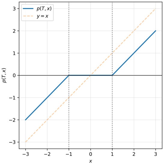
Figure 1. Soft-thresholding function $p(T,x)$. Observations with magnitude below the threshold T are mapped to zero, while larger values are shrunk toward zero by an amount T.

One of the popular methods for choosing a threshold in a thresholding problem is the universal threshold $T_{\mathrm{U}}=\sigma \sqrt{2lnN}$. Intuitively, the universal threshold is chosen such that, with a high probability, all noise coefficients are less than this value in absolute value. Indeed, if $Y_i$, $i=1,\dots ,N,$ have a normal distribution $\mathcal{N}(0,{\sigma }^2)$, then

$$\mathbb{P}\left(\underset{1\le i\le N}{max}\left|Y_i\right|>T_{\mathrm{U}}\right)\to 0.$$

(7)

Thus, the universal threshold ensures complete suppression of noise coefficients with an asymptotic probability of 1 and is the largest among the so-called useful thresholds (i.e., those that preserve significant signal coefficients but remove noise ones). In particular, any higher threshold will lead to excessive zeroing of informative coefficients.

Therefore, the universal threshold can be considered the upper limit of the range of rational (useful) thresholds. More details can be found in the monograph [16].

To quantitatively describe the reconstruction quality, we introduce the mean-square risk

$$R\left(T\right)=\sum _{i=1}^N\mathbb{E}{\left({\widehat{\mu }}_i-{\mu }_i\right)}^2,$$

(8)

which serves as a natural measure of the thresholding procedure’s efficiency. Minimizing $R\left(T\right)$ with respect to the parameter T leads to the definition of the optimal threshold

$$T_{min}=\arg \underset{T\in (0,T_U]}{min}R\left(T\right),$$

(9)

ensuring the smallest value of the mean-square deviation between the reconstructed and true signals. The value of $T_{min}$ depends on the unknown components ${\mu }_i$ and, therefore, cannot be calculated directly in practice.

To circumvent this difficulty, a risk estimate expressed in terms of observed data is used:

$$\widehat{R}\left(T\right)=\sum _{i=1}^{N}F(T,X_i),$$

(10)

where the function $F(T,X_i)$ is defined by the rule

$$F(T,X_i)=\left\{\begin{array}{cc}{X}_i^2-{\sigma }^2,\hfill & |X_i| \le T,\hfill \\ T^2+{\sigma }^2,\hfill & |X_i| > T.\hfill \end{array}\right.$$

(11)

It is easy to verify that the estimate constructed in this way is unbiased, that is, $\mathbb{E}\widehat{R}\left(T\right)=R\left(T\right)$.

Similarly, we define an adaptive threshold that minimizes the empirical risk estimate:

$$T_S=\arg \underset{T\in (0,T_U]}{min}\widehat{R}\left(T\right),$$

(12)

which is known in the literature as the SURE threshold (Stein’s Unbiased Risk Estimate threshold). The threshold $T_S$ is a random variable dependent on the observations $X_i$ and serves as a practical replacement for the theoretically optimal $T_{min}$.

In the following discussion, the classical Bernstein inequality [17] will be used to obtain probability estimates and upper bounds on risk:

$$\mathbb{P}\left(\sum _{i=1}^n{\xi }_i\ge t\right)\le exp\left(-{\displaystyle \frac{t^2/2}{{\sum }_{i=1}^n\mathbb{E}{\xi }_i^2+bt/3}}\right),t>0,$$

(13)

where $|{\xi }_i| \le b$ a.s. This inequality allows one to obtain exponential estimates for the tails of distributions and is widely used in the analysis of sums of independent random variables.

3. Theoretical Properties of the Risk and Its Estimation

3.1. Upper Bound for the Risk at the Optimal Threshold

In this section, we examine the asymptotic behavior of the risk in a sparse model defined by the condition $N{p}_N=o\left(N^{1-\gamma }\right)$. Under these assumptions, we show that the mean-square risk at the optimal threshold $T_{min}$ is of order $N^{1-\gamma }lnN$ at most. The main result is formulated in the following theorem.

Theorem 1.

Let the sparsity condition $N{p}_N=o\left(N^{1-\gamma }\right)$ be satisfied for some $\gamma \in (0,1)$ and let $T_{min}$ be the threshold that minimizes the theoretical risk $R\left(T\right)$. Then there exists a constant $C>0$ such that

$$R\left(T_{min}\right)\le C{N}^{1-\gamma }lnN.$$

(14)

Proof. 

Let’s split the risk into two parts:

$$\begin{array}{cc}\hfill R\left(T_{min}\right)& =\mathbb{E}\parallel \widehat{\mu }\left(T_{min}\right){-\mu \parallel }^2=\hfill \\ \hfill & =\mathbb{E}\parallel \widehat{\mu }\left(T_{min}\right){-\mu \parallel }^2(\mathbf{1}(N_0>N^{1-\gamma })+\mathbf{1}(N_0\le N^{1-\gamma }))=\hfill \\ \hfill & =\mathbb{E}[\parallel \widehat{\mu }\left(T_{min}\right){-\mu \parallel }^2\mathbf{1}(N_0>N^{1-\gamma })]+\mathbb{E}[{\parallel \widehat{\mu }\left(T_{min}\right)-\mu \parallel }^2\mathbf{1}(N_0\le N^{1-\gamma })].\hfill \end{array}$$

Consider the first part. We introduce the following notation:

$$Y=\parallel \widehat{\mu }\left(T_{min}\right){-\mu \parallel }^2,$$

(15)

$$A=\{N_0>N^{1-\gamma }\}.$$

(16)

In this notation, taking into account the upper bound for the terms in (8) from [18], we have:

$$\begin{array}{cc}\hfill \mathbb{E}\left(\right[\left|\right|\widehat{\mu }\left(T_{min}\right)-\mu \left|{|}^2\mathbf{1}(N_0>N^{1-\gamma })\right]\left|N_0\right)& =\mathbb{P}\left(A\right)·\mathbb{E}\left(Y\right|A)=\mathbb{P}\left(A\right)·\mathbb{E}\left(Y\right|N_0)\le \hfill \\ \hfill & \le cN{T}_U^2·\mathbb{P}(N_0>N^{1-\gamma })\hfill \end{array}$$

(17)

Using Bernstein’s inequality [17] and taking into account that $N{p}_N=o\left(N^{1-\gamma }\right)$, for $\mathbb{P}(N_0>N^{1-\gamma })$ we obtain

$$\begin{array}{cc}\hfill \mathbb{P}(N_0>N^{1-\gamma })& =\mathbb{P}(N_0-\mathbb{E}{N}_0>N^{1-\gamma }-\mathbb{E}{N}_0)\le \hfill \\ \hfill & \le exp(-c·{\displaystyle \frac{N^{2(1-\gamma )}}{N{p}_N(2+\frac{N^{1-\gamma }}{3N{p}_N})}})=exp(-c·{\displaystyle \frac{N^{2(1-\gamma )}}{2N{p}_N+N^{1-\gamma }/3}})\le \hfill \\ \hfill & \le exp(-c^{\prime }{N}^{1-\gamma })\hfill \end{array}$$

(18)

Now consider the second part.

$$\begin{array}{cc}\hfill \mathbb{E}[\parallel \widehat{\mu }\left(T_{min}\right){-\mu \parallel }^2\mathbf{1}(N_0\le N^{1-\gamma })]& =\mathbb{E}\left({\mathbb{E}}_z\right[\left|\right|\widehat{\mu }\left(T_{min}\right)-\mu \left|{|}^2\mathbf{1}(N_0\le N^{1-\gamma })\right]\left|N_0\right]).\hfill \end{array}$$

(19)

Since (18) has an exponential order of decrease, this term does not affect the order of $T_{min}$ and $R\left(T_{min}\right)$, therefore, using the method of proving Lemma 2 from [15], we can verify that $T_{min}\ge \sigma \sqrt{2\gamma lnN}-{\alpha }_n$, where $|{\alpha }_n|<c^{\prime }{\displaystyle \frac{lnlnN}{\sqrt{lnN}}}$. Next, using the reasoning of Theorem 2 from [14], we obtain the estimate

$$\begin{array}{c}\hfill \mathbb{E}({\mathbb{E}}_z\left[\right||\widehat{\mu }\left(T_{min}\right)-{\mu \left|\right|}^2\mathbf{1}(N_0\le N^{1-\gamma })]\left|N_0\right)\le c{N}^{1-\gamma }lnN,\end{array}$$

(20)

where c is some positive constant.

Combining the given estimates, we obtain the statement of the theorem. □

The resulting estimate defines the order of theoretical risk at the optimal threshold. Let us now turn to an analysis of the probabilistic properties of its empirical estimate $\widehat{R}\left(T\right)$.

3.2. Central Limit Theorem and Strong Law of Large Numbers for the Risk Estimate

Theorem 2.

Let the conditions of Theorem 1 be satisfied and $1/2<\gamma <1$. Then

$$\mathbb{P}\left({\displaystyle \frac{\widehat{R}\left(T_S\right)-R\left(T_{min}\right)}{{\sigma }^2\sqrt{2N}}}<x\right)\underset{N\to \infty }{\to }\Phi \left(x\right).$$

(21)

Proof. 

$$\begin{array}{cc}\hfill {\displaystyle \frac{\widehat{R}\left(T_S\right)-R\left(T_{min}\right)}{{\sigma }^2\sqrt{2N}}}& ={\displaystyle \frac{(\widehat{R}\left(T_S\right)-R\left(T_{min}\right))(\mathbf{1}(N_0>N^{1-\gamma })+\mathbf{1}(N_0\le N^{1-\gamma }))}{{\sigma }^2\sqrt{2N}}}=\hfill \\ \hfill & \equiv {\displaystyle \frac{(\widehat{R}\left(T_{min}\right)-R\left(T_{min}\right))\mathbf{1}(N_0\le N^{1-\gamma })}{{\sigma }^2\sqrt{2N}}}+U(T_S,T_{min}).\hfill \end{array}$$

(22)

Let us denote the first term by $z_N$ and consider the difference between the distribution function of $z_N$ and the distribution function of the standard normal law:

$$\begin{array}{cc}\hfill |\mathbb{P}(z_N<x)-\Phi \left(x\right)|& = |\sum _{k=0}^{\left[N^{1-\gamma }\right]}{p}_{Nk}·\mathbb{P}(z_N<x|N_0=k)-\Phi \left(x\right)|\le \hfill \\ \hfill & \le \sum _{k=0}^{\left[N^{1-\gamma }\right]}{p}_{Nk}·\left|\right(\mathbb{P}(z_N<x|N_0=k)-\Phi \left(x\right)|+\Phi \left(x\right)·\mathbb{P}(N_0>N^{1-\gamma })\le \hfill \\ \hfill & \le \underset{0\le k\le \left[N^{1-\gamma }\right]}{sup}\left|\right(\mathbb{P}(z_N<x|N_0=k)-\Phi \left(x\right)|\sum _{k=0}^{\left[N^{1-\gamma }\right]}{p}_{Nk}+exp(-c^{\prime }{N}^{1-\gamma }).\hfill \end{array}$$

(23)

Because of the sparsity conditions [19]

$$\begin{array}{c}\hfill \underset{N\to \infty }{lim}{\displaystyle \frac{\mathbb{D}(\widehat{R}\left(T_{min}\right)-R\left(T_{min}\right))}{{\sigma }^{4}2N}}=1,\end{array}$$

(24)

and since ${\displaystyle \sum _{k=0}^{\left[N^{1-\gamma }\right]}}{p}_{Nk}\le 1$, using the Berry-Esseen inequality for sums of differently distributed independent random variables, we obtain that as $N\to \infty$

$$\underset{x\in \mathbb{R}}{sup}\underset{0\le k\le \left[N^{1-\gamma }\right]}{sup}\left|\right(\mathbb{P}(z_N<x|N_0=k)-\Phi \left(x\right)|\to 0.$$

(25)

It remains to show that $U(T_S,T_{min})$ tends to zero in probability when $N\to \infty$.

$$\begin{array}{cc}\hfill U(T_S,T_{min})& ={\displaystyle \frac{\widehat{R}\left(T_S\right)-\widehat{R}\left(T_{min}\right)}{{\sigma }^2\sqrt{2N}}}+{\displaystyle \frac{(\widehat{R}\left(T_{min}\right)-R\left(T_{min}\right))\mathbf{1}(N_0>N^{1-\gamma })}{{\sigma }^2\sqrt{2N}}}.\hfill \end{array}$$

(26)

For the second term, arguing as in Theorem 1, we obtain the estimate

$$\begin{array}{c}\hfill \mathbb{P}\left(\left|{\displaystyle \frac{(\widehat{R}\left(T_{min}\right)-R\left(T_{min}\right))\mathbf{1}(N_0>N^{1-\gamma })}{{\sigma }^2\sqrt{2N}}}\right|>ϵ\right)\le \mathbb{P}(N_0>N^{1-\gamma })\le exp(-c^{\prime }{N}^{1-\gamma }).\end{array}$$

(27)

Let’s consider the first term.

$$\begin{array}{c}\hfill \mathbb{P}\left(\right|{\displaystyle \frac{\widehat{R}\left(T_S\right)-\widehat{R}\left(T_{min}\right)}{{\sigma }^2\sqrt{2N}}}·\mathbf{1}(N_0\le N^{1-\gamma })|>ϵ)=\\ \hfill =\sum _{k=0}^{\left[N^{1-\gamma }\right]}{p}_{Nk}\mathbb{P}\left(\right|{\displaystyle \frac{\widehat{R}\left(T_S\right)-\widehat{R}\left(T_{min}\right)}{{\sigma }^2\sqrt{2N}}}|>ϵ|N_0=k)\le \\ \hfill \le \underset{0\le k\le \left[N^{1-\gamma }\right]}{sup}\mathbb{P}\left(\right|{\displaystyle \frac{\widehat{R}\left(T_S\right)-\widehat{R}\left(T_{min}\right)}{{\sigma }^2\sqrt{2N}}}|>ϵ|N_0=k).\end{array}$$

(28)

Repeating the reasoning of Lemma 3 and Theorem 1 from [15], we verify that for any $ϵ>0$

$$\begin{array}{c}\hfill \underset{0\le k\le \left[N^{1-\gamma }\right]}{sup}\mathbb{P}\left(\right|{\displaystyle \frac{\widehat{R}\left(T_S\right)-\widehat{R}\left(T_{min}\right)}{{\sigma }^2\sqrt{2N}}}|>ϵ|N_0=k)\le \\ \hfill \le \underset{0\le k\le \left[N^{1-\gamma }\right]}{sup}\left(\mathbb{P}\left(T_S\le T^{*}|N_0=k\right)+\mathbb{P}\left(\underset{T\in [T^{*},T_U]}{sup}|{\displaystyle \frac{\widehat{R}\left(T\right)-\widehat{R}\left(T_{min}\right)}{{\sigma }^2\sqrt{2N}}}|>ϵ|N_0=k\right)\right),\end{array}$$

(29)

where $T^{*}=\sigma \sqrt{2\beta lnN}$ with an arbitrary $\beta \in (1,2\gamma )$, and each term tends to zero when $N\to \infty$. Thus,

$$\begin{array}{c}\hfill U(T_S,T_{min})\stackrel{\mathbb{P}}{⟶}0\mathrm{as}N\to \infty .\end{array}$$

(30)

The theorem is proved. □

Theorem 3.

Let the conditions of Theorem 1 be satisfied. For any $0<\gamma <1$, when $N\to \infty$

$${\displaystyle \frac{\widehat{R}\left(T_S\right)-R\left(T_{min}\right)}{N}}\stackrel{a.s.}{⟶}0$$

(31)

Proof. 

For any $ϵ>0$

$$\begin{array}{c}\hfill \mathbb{P}\left(\left|{\displaystyle \frac{\widehat{R}\left(T_S\right)-R\left(T_{min}\right)}{N}}\right|>ϵ\right)=\end{array}$$

$$\begin{array}{c}\hfill =\mathbb{P}\left(\left|{\displaystyle \frac{\widehat{R}\left(T_S\right)-R\left(T_{min}\right)}{N}}\right|>ϵ,N_0\le N^{1-\gamma }\right)+\\ \hfill +\mathbb{P}\left(\left|{\displaystyle \frac{\widehat{R}\left(T_S\right)-R\left(T_{min}\right)}{N}}\right|>ϵ,N_0>N^{1-\gamma }\right)\equiv \\ \hfill \equiv p_N+q_N.\end{array}$$

(32)

Next

$$\begin{array}{c}\hfill q_N\le \mathbb{P}\left(N_0>N^{1-\gamma }\right)\le exp(-c^{\prime }{N}^{1-\gamma })\end{array}$$

(33)

and hence ${\displaystyle \sum _{N=1}^{\infty }}{q}_N<\infty .$ For $p_N$ we have

$$\begin{array}{c}\hfill p_N=\sum _{k=0}^{\left[N^{1-\gamma }\right]}{p}_{Nk}\mathbb{P}\left(|{\displaystyle \frac{\widehat{R}\left(T_S\right)-R\left(T_{min}\right)}{N}}|>ϵ|N_0=k\right)\le \\ \hfill \le \underset{0\le k\le \left[N^{1-\gamma }\right]}{sup}\mathbb{P}\left(|{\displaystyle \frac{\widehat{R}\left(T_S\right)-R\left(T_{min}\right)}{N}}|>ϵ|N_0=k\right)\le \\ \hfill \le \underset{0\le k\le \left[N^{1-\gamma }\right]}{sup}\left(\mathbb{P}\left(T_S\le T^{*}|N_0=k\right)+\mathbb{P}\left(\underset{T\in [T^{*},T_U]}{sup}|{\displaystyle \frac{\widehat{R}\left(T\right)-\widehat{R}\left(T_{min}\right)}{N}}|>ϵ|N_0=k\right)\right),\end{array}$$

(34)

where $T^{*}=\sigma \sqrt{2\beta lnN}$ with an arbitrary $\beta \in (0,min\{1,2\gamma \left\}\right)$. Then arguing as in Lemma 3 and Theorem 2 of [15], we obtain that for some positive constants $c_1$, $c_2$, $C_1$ and $C_2$

$$\begin{array}{c}\hfill p_N\le C_{1}Nexp\left(-c_1{\displaystyle \frac{N^{1-\beta }}{{(lnN)}^3}}\right)+C_{2}exp\left(-c_2{\displaystyle \frac{N}{{(lnN)}^2}}\right)\end{array}$$

(35)

and ${\displaystyle \sum _{N=1}^{\infty }}{p}_N<\infty$. Thus,

$$\begin{array}{c}\hfill \sum _{N=1}^{\infty }(p_N+q_N)<\infty \end{array}$$

(36)

and by virtue of the Borel-Cantelli lemma the convergence (31) holds. □

4. Numerical Illustration: RTT Data Analysis

To illustrate the practical relevance of the proposed sparse observation model and the thresholding methodology, we present a numerical experiment based on real round-trip time (RTT) measurements collected in a controlled network probing setup. To clarify the overall processing pipeline used in the numerical experiment, Figure 2 presents a schematic overview of the main steps, from raw RTT measurements to sparse anomaly localization.

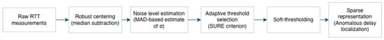
Figure 2. Schematic illustration of the data processing pipeline. Raw RTT measurements are centered using a robust location estimate, the noise level is estimated via a MAD-based procedure, an adaptive threshold is selected using the SURE criterion, and soft-thresholding is applied to obtain a sparse representation highlighting anomalous RTT components.

4.1. Data Acquisition and Preprocessing

RTT measurements were obtained by periodically sending batches of probe packets to a fixed network destination. Sending packets in batches allows reliable detection of packet losses and anomalous delays, while repeated probing with a fixed periodicity ensures temporal consistency of measurements.

All probes targeted the same network endpoint; therefore, the routing path can be assumed to be stable during the observation period. This allows abrupt RTT deviations to be interpreted primarily as manifestations of transient congestion or queueing effects, rather than route changes.

Each observation consists of a timestamp (in nanoseconds) and the corresponding RTT value (in milliseconds). Let ${\left\{RT{T}_i\right\}}_{i=1}^N$ denote the recorded sequence, where N = 54,000. To remove the constant delay component and obtain data compatible with the assumed noise model, the observations were centered with respect to the median value:

$$X_i=RT{T}_i-\mathrm{median}(RT{T}_1,\dots ,RT{T}_N).$$

(37)

The median was chosen as a robust baseline, since it is insensitive to rare but extremely large RTT values and preserves the approximate symmetry of the noise component.

The noise level $\sigma$ was estimated using the median absolute deviation (MAD) [16],

$$\widehat{\sigma }=1.4826·\mathrm{median}\left(\right|X_i\left|\right),$$

(38)

which yielded $\widehat{\sigma }\approx 0.45$ ms for the considered dataset.

4.2. Sparse Structure After Thresholding

Figure 3 illustrates the effect of thresholding on the centered RTT data. The original centered observations are shown together with the output of the continuous soft-thresholding function $p(T,X_i)$.

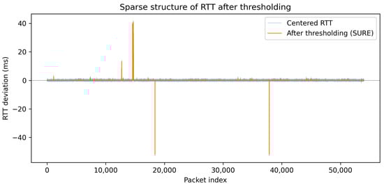
Figure 3. Sparse structure of RTT deviations after thresholding. The blue curve corresponds to centered RTT observations, while the orange curve shows the thresholded signal. Thresholding suppresses small-amplitude fluctuations attributed to noise, while preserving rare, high-magnitude deviations corresponding to anomalous network delays.

As predicted by the sparse observation model, the vast majority of coefficients are set to zero after thresholding, while only a small number of significant components remain nonzero. In the present experiment, only about $2.4\%$ of the observations retain nonzero values after thresholding, which is consistent with the Bernoulli-type sparsity assumption introduced in Section 2.

4.3. Empirical Risk Minimization

To demonstrate the adaptive threshold selection mechanism, we computed Stein’s unbiased risk estimate $\widehat{R}\left(T\right)$ over a range of threshold values. The search was restricted to the interval $(0,T_U]$, where

$$T_U=\widehat{\sigma }\sqrt{2lnN}$$

(39)

is the universal threshold. For the considered dataset, $T_U\approx 2.08$ ms.

Figure 4 shows the resulting empirical risk curve together with the selected SURE threshold $T_S$.

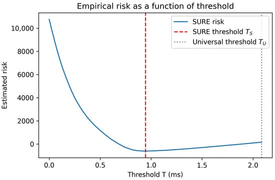
Figure 4. Empirical SURE risk $\widehat{R}\left(T\right)$ as a function of the threshold value T. The dashed vertical line indicates the data-driven threshold $T_S$ minimizing the empirical risk. The dotted vertical line corresponds to the universal threshold $T_U$.

The empirical risk curve exhibits a clear and well-defined minimum, illustrating the theoretical results on the existence and stability of an optimal threshold. In particular, overly small thresholds retain excessive noise, while overly large thresholds lead to the loss of informative signal components. The SURE-based procedure yields $T_S\approx 0.95$ ms in this experiment.

4.4. Summary Statistics

Table 1 reports summary statistics of the RTT data and the resulting sparse representation.

Table 1. Summary statistics of RTT data and thresholding results.

Quantity	Value	Units
Total number of observations N	54,000	–
Nonzero components after thresholding	1299	–
Sparsity level	2.4	%
Universal threshold $T_U$	2.08	ms
Selected threshold $T_S$	0.95	ms
Estimated noise standard deviation $\widehat{\sigma }$	0.45	ms

These results quantitatively confirm that RTT anomalies form a highly sparse structure, thereby supporting the modeling assumptions and validating the applicability of the proposed asymptotic analysis.

5. Conclusions

This paper presents an asymptotic analysis of the properties of the mean-square risk during threshold processing of noisy signals in a sparse stochastic observation model. For the theoretically optimal threshold that minimizes the theoretical risk, an upper bound is obtained, showing that the risk does not exceed a value of the order $N^{1-\gamma }lnN$.

Furthermore, a central limit theorem for the empirical risk estimate is established, as well as a strong law of large numbers, which guarantees the almost-everywhere convergence of the empirical risk to its theoretical counterpart. These results provide a rigorous theoretical basis for analyzing the asymptotic properties of thresholding procedures in problems of sparse signal recovery from observations with Gaussian noise.

The obtained estimates refine the classical results of Donoho and Johnstone (see [20]) and confirm the effectiveness of thresholding methods under sparsity conditions.

At the same time, the proposed analysis has several limitations. In particular, the theoretical results are derived under the assumption of independent Gaussian noise and rely on an asymptotic framework with a large number of observations. Moreover, the sparsity structure is characterized by a specific rate of decay of the proportion of nonzero components, which may not fully capture more complex or heterogeneous sparse patterns encountered in practice.

A promising direction for future research is to extend the proposed approach to more general models incorporating dependent noise, inhomogeneous variances, and multidimensional data structures. Another important direction is to study the asymptotic behavior of the optimal threshold under different sparsity regimes and to analyze the minimax properties of the resulting procedures. Finally, it would be of interest to investigate models with a random sample size, where the number of observations N is itself a random variable. Such settings naturally arise in practical applications, including network monitoring problems with random traffic intensity or missing observations, and may require new asymptotic tools for analyzing thresholding procedures and their associated risk.

References

- Borisov, A.V.; Kurinov, Y.N.; Smeliansky, R.L. Mathematical Support for Monitoring of States and Numerical Characteristics of Network Connection Based on Compound Statistical Information. Inform. Appl. 2025, 19, 35–44. [Google Scholar]
- Sawabe, A.; Shinohara, Y.; Iwai, T. Congestion State Estimation via Packet-Level RTT Gradient Analysis with Gradual RTT Smoothing. In Proceedings of the 2024 IEEE 21st Consumer Communications & Networking Conference (CCNC), Las Vegas, NV, USA, 6–9 January 2024; pp. 857–862. [Google Scholar]
- Mittal, R.; Lam, V.T.; Dukkipati, N.; Blem, E.; Wassel, H.; Ghobadi, M.; Vahdat, A.; Wang, Y.; Wetherall, D.; Zats, D. TIMELY: RTT-Based Congestion Control for the Datacenter. ACM SIGCOMM Comput. Commun. Rev. 2015, 45, 537–550. [Google Scholar] [CrossRef]
- Ancilotti, E.; Boetti, S.; Bruno, R. RTT-Based Congestion Control for the Internet of Things. In Wired/Wireless Internet Communication, Proceedings of the 16th IFIP WG 6.2 International Conference, WWIC 2018, Boston, MA, USA, 18–20 June 2018; Springer: Cham, Switzerland, 2018; pp. 3–15. [Google Scholar]
- Gao, H.-Y.; Bruce, A.G. Waveshrink with Firm Shrinkage. Stat. Sin. 1997, 7, 855–874. [Google Scholar]
- Gao, H.-Y. Wavelet Shrinkage Denoising Using the Non-Negative Garrote. J. Comput. Graph. Statist. 1998, 7, 469–488. [Google Scholar] [CrossRef]
- Marron, J.S.; Adak, S.; Johnstone, I.M.; Neumann, M.H.; Patil, P. Exact Risk Analysis of Wavelet Regression. J. Comput. Graph. Stat. 1998, 7, 278–309. [Google Scholar] [CrossRef]
- Poornachandra, S.; Kumaravel, N.; Saravanan, T.K.; Somaskandan, R. WaveShrink Using Modified Hyper-Shrinkage Function. In Proceedings of the 2005 IEEE Engineering in Medicine and Biology 27th Annual Conference, Shanghai, China, 17–18 January 2006; pp. 30–32. [Google Scholar]
- Abramovich, F.; Benjamini, Y.; Donoho, D.; Johnstone, I. Adapting to Unknown Sparsity by Controlling the False Discovery Rate. Ann. Statist. 2006, 34, 584–653. [Google Scholar] [CrossRef]
- Donoho, D.; Jin, J. Asymptotic Minimaxity of False Discovery Rate Thresholding for Sparse Exponential Data. Ann. Statist. 2006, 34, 2980–3018. [Google Scholar] [CrossRef]
- Markin, A.V. Limit Distribution of Risk Estimate of Wavelet Coefficient Thresholding. Inform. Appl. 2009, 3, 57–63. [Google Scholar]
- Huang, H.-C.; Lee, T.C.M. Stabilized Thresholding with Generalized Sure for Image Denoising. In Proceedings of the 2010 IEEE International Conference on Image Processing, Hong Kong, China, 26–29 September 2010; pp. 1881–1884. [Google Scholar]
- Zhao, R.-M.; Cui, H.-M. Improved Threshold Denoising Method Based on Wavelet Transform. In Proceedings of the 2015 7th International Conference on Modelling, Identification and Control (ICMIC 2015), Sousse, Tunisia, 18–20 December 2015; pp. 1–4. [Google Scholar]
- Vorontsov, M.O.; Shestakov, O.V. Mean-Square Risk of the FDR Procedure under Weak Dependence. Inform. Appl. 2023, 17, 34–40. [Google Scholar]
- Kudryavtsev, A.A.; Shestakov, O.V. Properties of the SURE Estimates When Using Continuous Thresholding Functions for Wavelet Shrinkage. Mathematics 2024, 12, 3646. [Google Scholar] [CrossRef]
- Mallat, S. A Wavelet Tour of Signal Processing; Academic Press: New York, NY, USA, 1999. [Google Scholar]
- Bennett, G. Probability Inequalities for the Sum of Independent Random Variables. J. Am. Stat. Assoc. 1962, 57, 33–45. [Google Scholar] [CrossRef]
- Donoho, D.; Johnstone, I.M. Ideal Spatial Adaptation via Wavelet Shrinkage. Biometrika 1994, 81, 425–455. [Google Scholar] [CrossRef]
- Palionnaya, S.I.; Shestakov, O.V. Asymptotic Properties of MSE Estimate for the False Discovery Rate Controlling Procedures in Multiple Hypothesis Testing. Mathematics 2020, 8, 1913. [Google Scholar] [CrossRef]
- Donoho, D.; Johnstone, I.M. Adapting to Unknown Smoothness via Wavelet Shrinkage. J. Amer. Stat. Assoc. 1995, 90, 1200–1224. [Google Scholar] [CrossRef]
Disclaimer/Publisher’s Note: The statements, opinions and data contained in all publications are solely those of the individual author(s) and contributor(s) and not of MDPI and/or the editor(s). MDPI and/or the editor(s) disclaim responsibility for any injury to people or property resulting from any ideas, methods, instructions or products referred to in the content. |
© 2025 by the authors. Licensee MDPI, Basel, Switzerland. This article is an open access article distributed under the terms and conditions of the Creative Commons Attribution (CC BY) license.