Partially Symmetric Regularized Two-Step Inertial Alternating Direction Method of Multipliers for Non-Convex Split Feasibility Problems

Abstract

This paper presents a partially symmetric regularized two-step inertial alternating direction method of multipliers for solving non-convex split feasibility problems (SFP), which adds a two-step inertial effect to each subproblem and includes an intermediate update term for multipliers during the iteration process. Under suitable assumptions, the global convergence is demonstrated. Additionally, with the help of the Kurdyka−Łojasiewicz (KL) property, which quantifies the behavior of a function near its critical points, the strong convergence of the proposed algorithm is guaranteed. Numerical experiments are performed to demonstrate the efficacy.

1. Introduction

The split feasibility problem (SFP) can be expressed in the following manner:

$$to find x\in C \mathrm{such} \mathrm{that} Ax\in Q,$$

(1)

where C is a closed convex set and Q is a non-convex closed set. A is a linear mapping from ${ℝ}^m$ to ${ℝ}^n$. The split feasibility problem (SFP) has been applied to address a diverse array of real-world challenges, including image denoising [1], CT image reconstruction [2], intensity-modulated radiation therapy (IMRT) [3,4,5], and Pareto front navigation in multi-criteria optimization [6]. Additionally, numerous iterative approaches have been used to address the split feasibility problem (SFP) [7,8,9,10]. The majority of existing techniques are designed for convex sets, but satisfying convexity requirements remains challenging in practice. Therefore, the primary objective of this paper will be the split feasibility problem (SPF), where the sets involved are not always convex.

The alternating direction method of multipliers (ADMM) [11] is a crucial method for solving the separable linear constrained problem, as follows:

$$\begin{array}{l}\min f(x)+g(y)\\ \mathrm{s}.\mathrm{t} Ax+By=b,\end{array}$$

(2)

where f: ${ℝ}^n\to ℝ\cup \{+\infty \}$ is a proper lower semi-continuous function, g: ${ℝ}^m\to ℝ$ is smooth, $A\in {ℝ}^{l\times n},B\in {ℝ}^{l\times m},b\in {ℝ}^l$. The augmented Lagrangian function for problem (2) is

$$L_{\beta }(x,y,\lambda )=f(x)+g(y)-<\lambda ,Ax+By-b>+{\displaystyle \frac{\beta }{2}}\parallel Ax+By-b{\parallel }^2,$$

where $\lambda \in {ℝ}^l$ is a Lagrangian multiplier and β > 0 is a penalty parameter. The classic iterative format of ADMM for solving problem (2) is as follows:

$$\left\{\begin{array}{l}{x}^{k+1}\in \arg \min \left\{L_{\beta }\left(x,y^k,{\lambda }^k\right)\right\},\\ y^{k+1}\in \arg \min \left\{L_{\beta }\left(x^{k+1},y,{\lambda }^k\right)\right\},\\ {\lambda }^{k+1}={\lambda }^k+\beta \left(A{x}^{k+1}+B{y}^{k+1}-b\right).\end{array}\right.$$

In recent years, research on the theory and algorithms of ADMM has become relatively comprehensive [12,13,14,15,16]. ADMM has been widely applied for solving convex optimization problems. However, when the objective function is non-convex, ADMM may not converge. To address this issue, we transform problem (1) into a separable problem with linear constraints, which makes it easier to solve. Two functions play a crucial role: the indication function and the distance function. Mathematically, given a non-empty closed set D in the d-dimensional Euclidean space ${ℝ}^n$, the indicator function is defined as follows:

$${\delta }_Q(y)=\left\{\begin{array}{l}0,if y\in Q,\\ +\infty ,otherwise.\end{array}\right.$$

The distance function of set C, represented by $d_C$: ${ℝ}^n\to ℝ$ is given by

$$d_C(x)={\inf }_x\{\parallel x-u\parallel :u\in C\},$$

where ${\delta }_Q(y)$ is obviously proper lower semi-continuous and $d_C(x)$ is smooth. When C is a closed convex set and Q is a non-convex closed set, the non-convex split feasibility problem can be reformulated as follows:

$$\begin{array}{c}{\min }_{x,y}f(x)+g(y)={\displaystyle \frac{1}{2}}\parallel x-P_C(x){\parallel }^2+{\delta }_Q(y)\\ s.t.Ax=y.\end{array}$$

(3)

This optimization problem is the sum of two non-negative functions, and their minimum value of zero can only be achieved under the condition of problem (1). Due to C being a convex closed set, f(x) is continuous, differentiable, and gradient-Lipschitz continuous. The augmented Lagrangian function for problem (3) is as follows:

$$L_{\beta }(x,y,\lambda )=f(x)+g(y)-<\lambda ,Ax-y>+{\displaystyle \frac{\beta }{2}}\parallel Ax-y{\parallel }^2.$$

In order to endow the ADMM algorithm with better theoretical properties, a number of researchers have carried out the following studies based on problem (3). Zhao et al. [17] considered the symmetric version of ADMM and selected different relaxation factors $\gamma$ and s, adding the intermediate update term of the Lagrange multiplier ${\lambda }^{k+{\displaystyle \frac{1}{2}}}$ during the algorithm iteration process:

$$\left\{\begin{array}{l}{y}^{k+1}\in \arg \min \left\{L_{\beta }\left(x^k,y,{\lambda }^k\right)+{\displaystyle \frac{1}{2}}\parallel y-y^k{\parallel }_G^2\right\},\\ {\lambda }^{k+{\displaystyle \frac{1}{2}}}={\lambda }^k-\gamma \beta \left(A{x}^k-y^{k+1}\right),\\ x^{k+1}\in \arg \min \left\{L_{\beta }\left(x,y^{k+1},{\lambda }^{k+{\displaystyle \frac{1}{2}}}\right)\right\},\\ {\lambda }^{k+1}={\lambda }^{k+{\displaystyle \frac{1}{2}}}-s\beta \left(A{x}^{k+1}-y^{k+1}\right).\end{array}\right.$$

In addition, the combination of the ADMM algorithm with inertial technology can also significantly improve the performance of the ADMM algorithm in solving non-convex optimization problems. Dang et al. [18] incorporated the inertial technique into each sub-problem of the ADMM algorithm and employed a dual-relaxed term to ensure the convergence of the algorithm.

Based on the previous work, we propose a partially symmetric regularized two-step inertial alternating direction method of multipliers for solving the non-convex split feasibility problem, which has not been extensively studied in the past. The novelty of this paper can be summarized as follows: Firstly, we transform such type of non-convex split feasibility problems into two separable non-convex linear constraint problems for an easier solution. Secondly, we add an intermediate update term for the multipliers throughout the iteration phase and apply the two-step inertial technique to each sub-problem of the Alternating Direction Method of Multipliers (ADMM) algorithm. Lastly, to guarantee the strong convergence of the proposed algorithm for resolving non-convex split feasibility problems, we employ the Kurdyka−Łojasiewicz (KL) property.

The structure of the paper is as follows: The basic concepts, definitions, and related results are described in the second part. The convergence of the algorithm is demonstrated in the Section 3. The fourth part showcases the effectiveness of the algorithms through experiments. The Section 5 presents the main conclusions.

2. Preliminaries

In this article, ${ℝ}^n$ represents an n dimensional Euclidean space and $‖ . ‖$ represents the Euclidean norm. For any $x,y\in {ℝ}^n,⟨x,y⟩=x^{\top }$$y.\parallel x{\parallel }_G=\sqrt{x^{T}Gx}$, where $G\succ (\succ )0$ is a symmetric positive semidefinite matrix. ${\lambda }_{\min }(G)$ and ${\lambda }_{\max }(G)$ represent the minimum and maximum eigenvalues of the symmetric matrix G, respectively. Then, ${\lambda }_{\min }(G)\parallel y{\parallel }^2\le \parallel y{\parallel }_G^2\le {\lambda }_{\max }(G)\parallel y{\parallel }^2,$$for \forall y\in {ℝ}^n$. When set $Q\subset {ℝ}^n$ is non-empty, for any point $y\subset {ℝ}^n$, the distance from point y to set Q is defined as $d(x,Q)=$$\inf \{\parallel x-y\parallel \mid y\in Q\}$. In particular, if Q = ∅, then d(y, Q) = +∞. The domain of function g is denoted as dom g = {$y\in {ℝ}^n:g(y)<+\infty$}. In the Euclidean space, let C be a non-empty closed subset. The projection on the set C is the operator $P_C(x):{ℝ}^n\to C,$ which is defined as $P_C(x)=\arg \min \{\parallel u-x\parallel :u\in C\}$.

Definition 1 

([19]). If function g: ${ℝ}^n\to ℝ\cup \{+\infty \}$ satisfies $g\left(y_0\right)\le \lim \hspace{0.17em}{\inf }_{y\to y_0}g(y)$ at $y_0$, then function g is said to be lower semi-continuous at y. If g is lower semi-continuous at every point, then g is called a lower semi-continuous function. Due to Q being a closed set, g(y), y  $\in$ Q is a normal lower semi-continuous function.

Definition 2 

([19]). Let the function g: ${ℝ}^n\to ℝ\cup \{+\infty \}$ be normal lower semi-continuous.

(I) 

The Fréchet subdifferentiation of g at y $\in$ dom g is defined as

$$\widehat{\mathsf{\partial }}g(y)=\left\{y^{\ast }\in {ℝ}^n:\underset{x\ne y}{\lim } \underset{x\to y}{\inf }{\displaystyle \frac{g(x)-g(y)-⟨y^{\ast },x-y⟩}{\parallel x-y\parallel }}\ge 0\right\}.$$

(II) 

The limit subdifferentiation of g at y $\in$ dom g is defined as

$$\mathsf{\partial }g(y)=\left\{y^{\ast }\in {ℝ}^n:\mathsf{\exists }{y}_k\to y,g\left(y_k\right)\to g(y),{\widehat{y}}_k\in \widehat{\mathsf{\partial }}g(y),{\widehat{y}}_k\to y^{\ast }\right\}.$$

Note: The properties of several subdifferentials (see [19]) are listed as follows:

(I) 

$\forall y\in {ℝ}^n,\widehat{\mathsf{\partial }}g(y)\subseteq \mathsf{\partial }g(y) \mathrm{and} \widehat{\mathsf{\partial }}g(y)$ is a closed convex set, $\mathsf{\partial }g(y)$  is a closed set.

(II) 

If $y_k^{\ast }\subseteq \widehat{\mathsf{\partial }}g(y) \mathrm{and}\underset{y\to \infty }{\lim }\left(y_k,y_k^{\ast }\right)=\left(y,y^{\ast }\right)$, then $y^{\ast }\subseteq \mathsf{\partial }g(y)$.

(III) 

If $y\in {ℝ}^n$ is the minimum point of g, then $0\in \mathsf{\partial }g(y)$; if $0\in \mathsf{\partial }g(y)$, then y is the stable point of function g. The set of stable points of function g is denoted as crit g.

(IV) 

For any y $\in$ dom g, we get $\mathsf{\partial }(f(x)+g(y))=\mathsf{\nabla }f(x)+\mathsf{\nabla }g(y)$ if $g:{ℝ}^n\to ℝ\cup \{+\infty \}$ is normal lower semi-continuous and $f:{ℝ}^n\to ℝ\cup \{+\infty \}$ is continuous differentiable.

Definition 3. 

$\left\{{\omega }^{\ast }=\left(x^{\ast },y^{\ast },{\lambda }^{\ast }\right)\right\}$ is the stable point of the augmented Lagrangian function $L_{\beta }\mathsf{(}x$, y, λ) for problem (1), i.e., $0\in \mathsf{\partial }{L}_{\beta }({\omega }^{*})$, if and only if

$$\left\{\begin{array}{l}-{\lambda }^{\ast }\in \mathsf{\partial }g\left(y^{\ast }\right),\\ \mathsf{\nabla }f\left(x^{\ast }\right)=A^T{\lambda }^{\ast },\\ A{x}^{\ast }-y^{\ast }=0.\end{array}\right.$$

Definition 4 

([20]). (Kurdyka−Łojasiewicz property) The function $g:{ℝ}^n\to ℝ\cup \{+\infty \}$ is a normal lower semi-continuous function, let $-\infty <\eta \le +\infty$, denoted as $[{\eta }_1<f<{\eta }_2]$ and g is said to have KL property in $y^{\ast }\in dom \mathsf{\partial }g.$ If there exists $\eta$ $\in$ (0, +∞], a certain rain $U$ of y and a continuous concave function $\phi$: [0,$\eta$)→${ℝ}_{+}$, such that

(I) 

$\phi (0)=0$.

(II) 

$\phi$ is continuously differentiable on (0, $\eta$) and $\phi$ is also continuous at 0.

(III) 

$\forall s\in (0,\eta ),{\phi }^{\prime }(s)>0$.

(IV) 

$\forall y\in U\cap [g\left(y^{\ast }\right)<g<g\left(y^{\ast }\right)+\eta ]$, all KL inequalities hold:

$${\phi }^{\prime }\left(g(y)-g\left(y^{\ast }\right)\right)d(0,\mathsf{\partial }g(y))\ge 1.$$

Lemma 1 

([21]). (Consistent KL property) Assuming Ω is a compact set and function g: ${ℝ}^n\to$$ℝ\cup \{+\infty \}$ is a normal lower semi-continuous function. If the function g is a constant on Ω and satisfies the KL property at every point in Ω, then there exists $\epsilon >0,\eta >0,\phi \in {\varphi }_n$ such that for any $\overline{y}$ ∈ Ω and any y, they belong to the following intersection

$$\{y\in {ℝ}^n:d(y,\mathsf{\Omega })<\epsilon \}\cap [g(\overline{y})<g<g(\overline{y})+\eta \}$$

With

$${\phi }^{\prime }(g(y)-g(\overline{y}))d(0,\mathsf{\partial }g(y))\ge 1.$$

In some practical applications, many functions satisfy the KL property, such as semi-algebraic functions, real analytic functions, sub analytic functions, and strongly convex functions, as seen in reference [22].

Lemma 2 

([23]). If $\psi$: ${ℝ}^n\to ℝ\cup \{+\infty \}$ is a continuous differentiable function and $\nabla \psi$ is Lipschitz continuous, then there exists a Lipschitz constant $L_{\psi }$ > 0, such that for any x, y $\in {ℝ}^n$, there is:

$$\mid \psi (x)-\psi (y)-⟨\mathsf{\nabla }\psi (y),x-y⟩\mid \le {\displaystyle \frac{L_{\psi }}{2}}\parallel x-y{\parallel }^2.$$

Definition 5. 

(Sets and functions in semi-algebra)

(I) 

If there are a finite number of real polynomial functions $g_{ij},h_{ij}:{ℝ}^n\to ℝ$, such that

$$S={\displaystyle \underset{j=1}{\overset{p}{\cup }}{\displaystyle \underset{i=1}{\overset{q}{\cap }}\{u\in {ℝ}^n:g_{ij}(u)=0 \mathrm{and} h_{ij}(u)<0\}}},$$

then a subset S of ${ℝ}^n$ is a real semi-algebraic set.

(II) 

A funtion f: ${ℝ}^n$→(−∞, +∞] is called semi-algebraic if its graph

$$\left\{(u,t)\in {ℝ}^{n+1}:h(u)=t\right\}$$

is a semi-algebraic subset of ${ℝ}^{n+1}$.

Definition 6. 

(Cauchy–Schwarz inequality) If and only if x and y are linearly dependent, for $\forall x,y\in {ℝ}^n$, we have $\mid x^{T}y\mid \le \parallel x\parallel \cdot \parallel y\parallel$.

3. Split Feasibility Problem

3.1. Assumptions

Some assumptions and conditions about problem (3) are listed below.

(1)

$\gamma +s>0$ and $\gamma (1-2s)+s-6{(1-s)}^2>0$.

The solution set gram of this inequality system is represented as $(\gamma ,s)\in D=D_1\cup D_2$, where

$$D_1=\left({\displaystyle \frac{6{(1-s)}^2-s}{1-2s}},+\infty \right)\times \left(-\infty ,{\displaystyle \frac{1}{2}}\right)$$

and

$$D_2=\left(-s,{\displaystyle \frac{6{(1-s)}^2-s}{1-2s}}\right)\times \left({\displaystyle \frac{3-\sqrt{3}}{2}},{\displaystyle \frac{3+\sqrt{3}}{2}}\right)$$

Note: It can be seen that (γ, s) has a wide range of choices. Specifically, when $s\in ({\displaystyle \frac{3}{4}},1)$ occurs, $\gamma =(s,s)\in D_2$ the parameters γ and s of the proposed algorithm can take the same value in this interval.

(2)

$\beta >{\beta }_0={\displaystyle \frac{(\gamma +s)+\sqrt{{(\gamma +s)}^2+24\left[\gamma (1-2s)+s-6{(1-s)}^2\right]}}{2\left[\gamma (1-2s)+s-6{(1-s)}^2\right]}}>0.$

(3)

Note $\delta =\min \{{\delta }_1,{\delta }_2\}$, where,

$${\delta }_1=({\displaystyle \frac{1}{2}}{\lambda }_{\min }(G)-{\displaystyle \frac{\begin{array}{l}[(2s^2{\beta }^2+3)(1+s\beta +\tau +4\theta )\\ +(2{\gamma }^2{\beta }^2+2)(1+\gamma \beta -\tau +4\theta )](2\parallel A{\parallel }^2{\beta }^2{(1-s)}^2+\theta )\end{array}}{{(\gamma +s)}^2\beta }}-{\theta }^2-2\theta )>0,$$

$$\begin{array}{ll}\hfill {\delta }_2=& (-{\displaystyle \frac{\begin{array}{l}(2s^2{\beta }^2+3)(1+s\beta +\tau +4\theta )(4{\left(L+\parallel A{\parallel }^2(1-s)\beta \right)}^2+(s\beta +\tau ){‖A‖}^2+2\theta )\\ +(2{\gamma }^2{\beta }^2+2)(1+\gamma \beta +\tau +4\theta )(4{\left(L+\parallel A{\parallel }^2(1-s)\beta \right)}^2+(\gamma \beta -\tau ){‖A‖}^2+2\theta )\end{array}}{2{(\gamma +s)}^2\beta }}\hfill \\ & -{\displaystyle \frac{L+(2{\tau }^2-\beta )\parallel A{\parallel }^2+3}{2}}-2{\theta }^2)>0.\hfill \end{array}$$

(4)

Note $\theta >\max \left\{{\theta }_{1k,}{\theta }_{2k,}\right\}$ and $\left\{\right\{{\theta }_{1k}\},\{{\theta }_{2k}\},\{\tau \left\}\right\}\subseteq (0,1)$.  $\left\{{\theta }_{1k}\right\}$ and $\left\{{\theta }_{2k}\right\}$ are fixed constants.

(5)

C, Q are both semi-algebraic sets.

(6)

f is lg-Lipschitz differentiable, i.e., $\parallel \mathsf{\nabla }f(u)-\mathsf{\nabla }f(v)\parallel \le l_g\parallel u-v\parallel \mathrm{for} \mathrm{all} u,v\in {ℝ}^p\times {ℝ}^q.$

(7)

g is proper lower semi-continuous.

(8)

The set $\left\{{\omega }^k\in X\mid L_{\beta }(\omega )\le L_{\beta }\left({\omega }^0\right)\right\}$ is bounded.

3.2. Algorithm

For Algorithm 1 (PSRTADMM), its optimal conditions are as follows:

$$0\in \mathsf{\partial }g\left(y^{k+1}\right)+{\lambda }^k+\beta \left(A{x}^k-y^{k+1}\right)+G\left(y^{k+1}-y^k\right)+{\theta }_{1k}(y^{k-1}-y^k)+{\theta }_{2k}(y^{k-2}-y^{k-1})$$

(4)

$${\lambda }^{k+{\displaystyle \frac{1}{2}}}={\lambda }^k-\gamma \beta \left(A{x}^k-y^{k+1}\right)-{\theta }_{1k}(y^{k-1}-y^k)-{\theta }_{2k}(y^{k-2}-y^{k-1})$$

(5)

$$\begin{array}{cc}\hfill 0=& \mathsf{\nabla }f\left(x^{k+1}\right)-A^T{\lambda }^{k+{\displaystyle \frac{1}{2}}}+\beta A^T\left(A{x}^{k+1}-y^{k+1}\right)+\tau A^T(A{x}^{k+1}-A{x}^k)+{\theta }_{1k}{A}^T(x^{k-1}-x^k)\hfill \\ & +{\theta }_{2k}{A}^T(x^{k-2}-x^{k-1})\hfill \end{array}$$

(6)

$${\lambda }^{k+1}={\lambda }^{k+{\displaystyle \frac{1}{2}}}-s\beta \left(A{x}^{k+1}-y^{k+1}\right)-\tau (A{x}^{k+1}-A{x}^k)-{\theta }_{1k}A(x^{k-1}-x^k)-{\theta }_{2k}A(x^{k-2}-x^{k-1})$$

(7)

Algorithm 1 Partially Symmetric Regularized Two-step Inertial Alternating Direction Method of Multipliers for Non-convex Split Feasibility Problems (PSRTADMM)

$$\begin{gathered} \begin{array}{c}\mathrm{Step} 0. x_0\in {ℝ}^n,y_0\in {ℝ}^n,{\lambda }_0\in {ℝ}^n,\left(x^{-2},y^{-2}\right)=\left(x^{-1},y^{-1}\right)=\left(x^0,y^0\right) \mathrm{and} \beta > 0 \mathrm{are} \mathrm{given}; \mathrm{set} k: = 0\hfill \\ \mathrm{Step} 1. \mathrm{Find} y^{k+1}\in {ℝ}^n \mathrm{by} \mathrm{solving}\hfill \\ y^{k+1}\in \arg \min \{L_{\beta }(x^k,y,{\lambda }^k)+{\displaystyle \frac{1}{2}}{‖y-y^k‖}_G^2+{\theta }_{1k}<y,y^{k-1}-y^k>+{\theta }_{2k}<y,y^{k-2}-y^{k-1}>\hfill \\ G=\tau I-\beta A^{T}A, \mathrm{where} \mathrm{G} \in {ℝ}^{n\times n} \mathrm{is} \mathrm{symmetric} \mathrm{positive} \mathrm{definite} \mathrm{matrix}.\hfill \\ \mathrm{Step} 2. \mathrm{Find} {\lambda }^{k+{\displaystyle \frac{1}{2}}} \mathrm{by} \mathrm{solving}\hfill \\ {\lambda }^{k+{\displaystyle \frac{1}{2}}}={\lambda }^k-\gamma \beta (A{x}^k-y^{k+1})-{\theta }_{1k}(y^{k-1}-y^k)-{\theta }_{2k}(y^{k-2}-y^{k-1})\\ \mathrm{Step} 3. \mathrm{Find} x^{k+1} \mathrm{by} \mathrm{solving}\hfill \\ x^{k+1}\in \arg \min \{L_{\beta }(x,y^{k+1},{\lambda }^{k+{\displaystyle \frac{1}{2}}})+{\displaystyle \frac{\tau }{2}}{‖Ax-A{x}^k‖}^2+{\theta }_{1k}<Ax,A(x^{k-1}-x^k)> \\ +{\theta }_{2k}<Ax,A(x^{k-2}-x^{k-1})>\}\\ \mathrm{Step} 4. \mathrm{Find} {\lambda }^{k+1} \mathrm{by} \mathrm{solving}\hfill \\ {\lambda }^{k+1}={\lambda }^{k+{\displaystyle \frac{1}{2}}}-s\beta (A{x}^k-y^{k+1})-\tau (A{x}^{k+1}-A{x}^k)-A{\theta }_{1k}(x^{k-1}-x^k)-A{\theta }_{2k}(x^{k-2}-x^{k-1})\\ \mathrm{If} \mathrm{the} \mathrm{stopping} \mathrm{criterion} \mathrm{is} \mathrm{satisfied}, \mathrm{then} \mathrm{stop}; \mathrm{else}, \mathrm{go} \mathrm{to} \mathrm{Step} 1 \mathrm{with} k: = k + 1 .\hfill \end{array} \end{gathered}$$

3.3. Convergence Analysis

Next, we establish the convergence analysis of the proposed algorithm. Lemma 3 below indicates that the sequence {$L_{\beta }({\omega }^k)$} monotonically decreases. For ease of analysis, z = (x, y).

Lemma 3. 

If Assumptions holds, then

$$\mathcal{L}\left({\tilde{\omega }}^{k+1}\right)+\delta \parallel z^{k+1}-z^k{\parallel }^2\le \mathcal{L}\left({\tilde{\omega }}^k\right).$$

Proof. 

Firstly, from the optimality conditions of Equations (5) and (7), we can obtain

$$\begin{array}{l}{L}_{\beta }\left(x^{k+1},y^{k+1},{\lambda }^{k+1}\right)\\ =L_{\beta }\left(x^{k+1},y^{k+1},{\lambda }^{k+{\displaystyle \frac{1}{2}}}\right)-<{\lambda }^{k+1}-{\lambda }^{k+{\displaystyle \frac{1}{2}}},A{x}^{k+1}-y^{k+1}>\\ =L_{\beta }\left(x^{k+1},y^{k+1},{\lambda }^{k+{\displaystyle \frac{1}{2}}}\right)+<s\beta (A{x}^{k+1}-y^{k+1})+\tau (A{x}^{k+1}-A{x}^k)+{\theta }_{1k}A(x^{k-1}-x^k)\\ +{\theta }_{2k}A(x^{k-2}-x^{k-1}),A{x}^{k+1}-y^{k+1}>\end{array}$$

$$\begin{array}{l}\le L_{\beta }\left(x^{k+1},y^{k+1},{\lambda }^{k+{\displaystyle \frac{1}{2}}}\right)+<s\beta (A{x}^{k+1}-y^{k+1}),A{x}^{k+1}-y^{k+1}>+<\tau (A{x}^{k+1}-A{x}^k),A{x}^{k+1}-y^{k+1}>\\ +<{\theta }_{1k}A(x^{k-1}-x^k),A{x}^{k+1}-y^{k+1}>+<{\theta }_{2k}A(x^{k-2}-x^{k-1}),A{x}^{k+1}-y^{k+1}>\\ \le L_{\beta }\left(x^{k+1},y^{k+1},{\lambda }^{k+{\displaystyle \frac{1}{2}}}\right)+{\displaystyle \frac{2s^2{\beta }^2+3}{2}}{‖A{x}^{k+1}-y^{k+1}‖}^2+{\displaystyle \frac{{\tau }^2{‖A‖}^2}{2}}{‖x^{k+1}-x^k‖}^2\\ +{\displaystyle \frac{{\theta }^2{‖A‖}^2}{2}}{‖x^{k-1}-x^k‖}^2+{\displaystyle \frac{{\theta }^2{‖A‖}^2}{2}}{‖x^{k-2}-x^{k-1}‖}^2\end{array}$$

(8)

And

$$\begin{array}{l}{L}_{\beta }\left(x^k,y^{k+1},{\lambda }^{k+{\displaystyle \frac{1}{2}}}\right)\\ =L_{\beta }\left(x^k,y^{k+1},{\lambda }^k\right)-<{\lambda }^{k+{\displaystyle \frac{1}{2}}}-{\lambda }^k,A{x}^k-y^{k+1}>\\ =L_{\beta }\left(x^k,y^{k+1},{\lambda }^k\right)+<\gamma \beta (A{x}^{k+1}-y^{k+1})+{\theta }_{1k}(y^{k-1}-y^k)+{\theta }_{2k}(y^{k-2}-y^{k-1}),A{x}^k-y^{k+1}>\\ \le L_{\beta }\left(x^k,y^{k+1},{\lambda }^k\right)+<\gamma \beta (A{x}^{k+1}-y^{k+1}),A{x}^k-y^{k+1}>+<{\theta }_{1k}(y^{k-1}-y^k),A{x}^k-y^{k+1}>\\ +<{\theta }_{2k}(y^{k-2}-y^{k-1}),A{x}^k-y^{k+1}>\\ \le L_{\beta }\left(x^k,y^{k+1},{\lambda }^k\right)+({\gamma }^2{\beta }^2+1){‖A{x}^k-y^{k+1}‖}^2+{\displaystyle \frac{{\theta }^2}{2}}{‖y^{k-1}-y^k‖}^2+{\displaystyle \frac{{\theta }^2}{2}}{‖y^{k-2}-y^{k-1}‖}^2\end{array}$$

(9)

On the other hand, by the definition of augmented Lagrangian functions, the optimality condition of Equation (6), Lipschitz continuity, and Lemma 2 of $\nabla$f, we have

$$\begin{array}{l}{L}_{\beta }\left(x^{k+1},y^{k+1},{\lambda }^{k+{\displaystyle \frac{1}{2}}}\right)-L_{\beta }\left(x^k,y^{k+1},{\lambda }^{k+{\displaystyle \frac{1}{2}}}\right)\\ =f\left(x^{k+1}\right)-f\left(x^k\right)-{\displaystyle \frac{\beta }{2}}\parallel A{\parallel }^2\parallel x^{k+1}-x^k{\parallel }^2-<{\lambda }^{k+{\displaystyle \frac{1}{2}}}-\beta \left(A{x}^{k+1}-y^{k+1}\right),A{x}^{k+1}-A{x}^k>\\ =f\left(x^{k+1}\right)-f\left(x^k\right)-{\displaystyle \frac{\beta }{2}}\parallel A{\parallel }^2\parallel x^{k+1}-x^k{\parallel }^2-<\mathsf{\nabla }f\left(x^{k+1}\right),x^{k+1}-x^k>\\ -<\tau (A{x}^{k+1}-A{x}^k),x^{k+1}-x^k>-<{\theta }_{1k}A(x^{k-1}-x^k),x^{k+1}-x^k>\\ -<{\theta }_{2k}A(x^{k-2}-x^{k-1}),x^{k+1}-x^k>\\ \le {\displaystyle \frac{L+({\tau }^2-\beta )\parallel A{\parallel }^2+3}{2}}\parallel x^{k+1}-x^k{\parallel }^2+{\displaystyle \frac{{\theta }^2{‖A‖}^2}{2}}{‖x^{k-1}-x^k‖}^2+{\displaystyle \frac{{\theta }^2{‖A‖}^2}{2}}{‖x^{k-2}-x^{k-1}‖}^2\end{array}$$

(10)

Given $y^{k+1}$ is the optimal solution of (4), it follows that

$$\begin{array}{l}{L}_{\beta }\left(x^k,y^{k+1},{\lambda }^k\right)-L_{\beta }\left(x^k,y^k,{\lambda }^k\right)\\ \le -{\displaystyle \frac{1}{2}}\parallel y^{k+1}-y^k{\parallel }_G^2-{\theta }_{1k}<y^{k-1}-y^k,y^k-y^{k+1}>-{\theta }_{2k}<y^{k-2}-y^{k-1},y^k-y^{k+1}>\\ \le (\theta -{\displaystyle \frac{1}{2}}{\lambda }_{\min }(G))\parallel y^{k+1}-y^k{\parallel }^2+{\displaystyle \frac{\theta }{2}}{‖y^{k-1}-y^k‖}^2+{\displaystyle \frac{\theta }{2}}{‖y^{k-2}-y^{k-1}‖}^2\end{array}$$

(11)

Therefore, adding Equations (8)–(11), we have

$$\begin{array}{l}{L}_{\beta }\left(x^{k+1},y^{k+1},{\lambda }^{k+1}\right)-L_{\beta }\left(x^k,y^k,{\lambda }^k\right)\\ \le {\displaystyle \frac{L+(2{\tau }^2-\beta )\parallel A{\parallel }^2+3}{2}}\parallel x^{k+1}-x^k{\parallel }^2+(\theta -{\displaystyle \frac{1}{2}}{\lambda }_{\min }(G))\parallel y^{k+1}-y^k{\parallel }^2\\ +{\theta }^2{‖A‖}^2{‖x^{k-1}-x^k‖}^2+{\theta }^2{‖A‖}^2{‖x^{k-2}-x^{k-1}‖}^2+{\displaystyle \frac{{\theta }^2+\theta }{2}}{‖y^{k-1}-y^k‖}^2+{\displaystyle \frac{{\theta }^2+\theta }{2}}{‖y^{k-2}-y^{k-1}‖}^2\\ +{\displaystyle \frac{2s^2{\beta }^2+3}{2}}{‖A{x}^{k+1}-y^{k+1}‖}^2+({\gamma }^2{\beta }^2+1){‖A{x}^k-y^{k+1}‖}^2\end{array}$$

(12)

In addition, it can be obtained from Step 2 and Step 4 of Algorithm 1 that

$$\begin{array}{l}A{x}^k-y^{k+1}={\displaystyle \frac{1}{(\gamma +s)\beta }}\left({\lambda }^k-{\lambda }^{k+1}\right)-{\displaystyle \frac{s\beta +\tau }{(\gamma +s)\beta }}\left(A{x}^{k+1}-A{x}^k\right)\\ -{\displaystyle \frac{1}{(\gamma +s)\beta }}({\theta }_{1k}A(x^{k-1}-x^k)+{\theta }_{2k}A(x^{k-2}-x^{k-1})+{\theta }_{1k}(y^{k-1}-y^k)+{\theta }_{2k}(y^{k-2}-y^{k-1}))\end{array}$$

(13)

$$\begin{array}{l}A{x}^{k+1}-y^{k+1}={\displaystyle \frac{1}{(\gamma +s)\beta }}\left({\lambda }^k-{\lambda }^{k+1}\right)+{\displaystyle \frac{\gamma \beta -\tau }{(\gamma +s)\beta }}\left(A{x}^{k+1}-A{x}^k\right)\\ -{\displaystyle \frac{1}{(\gamma +s)\beta }}({\theta }_{1k}A(x^{k-1}-x^k)+{\theta }_{2k}A(x^{k-2}-x^{k-1})+{\theta }_{1k}(y^{k-1}-y^k)+{\theta }_{2k}(y^{k-2}-y^{k-1}))\end{array}$$

(14)

On the other hand, it can be concluded from Step 4 of Algorithm 1 and (6) that:

$$A^T{\lambda }^{k+1}=\mathsf{\nabla }f\left(x^{k+1}\right)+A^T\beta (1-s)\left(A{x}^{k+1}-y^{k+1}\right)$$

(15)

Combining the Lipschitz continuity of $\nabla$f, we obtain

$$\begin{array}{l}\parallel A^T\parallel \parallel {\lambda }^{k+1}-{\lambda }^k\parallel \hfill \\ \le \left(L+\parallel A{\parallel }^2(1-s)\beta \right)\parallel x^{k+1}-x^k\parallel +\parallel A^T\parallel \beta (1-\gamma )\parallel y^{k+1}-y^k\parallel \hfill \end{array}$$

(16)

Furthermore, by applying the Cauchy inequality to (16), we have

$$\begin{array}{l}\parallel A{\parallel }^2\parallel {\lambda }^{k+1}-{\lambda }^k{\parallel }^2\\ \le 4{\left(L+\parallel A{\parallel }^2(1-s)\beta \right)}^2\parallel x^{k+1}-x^k{\parallel }^2+4\parallel A{\parallel }^2{\beta }^2{(1-s)}^2\parallel y^{k+1}-y^k{\parallel }^2\end{array}$$

(17)

So, combining Equations (13), (14) and (17), one has

$$\begin{array}{l}{\displaystyle \frac{2s^2{\beta }^2+3}{2}}{‖A{x}^{k+1}-y^{k+1}‖}^2+({\gamma }^2{\beta }^2+1){‖A{x}^k-y^{k+1}‖}^2\\ \le {\displaystyle \frac{(2s^2{\beta }^2+3)(1+s\beta +\tau +4\theta )+(2{\gamma }^2{\beta }^2+2)(1+\gamma \beta -\tau +4\theta )}{2{(\gamma +s)}^2\beta }}\parallel {\lambda }^{k+1}-{\lambda }^k{\parallel }^2\\ +{\displaystyle \frac{(2s^2{\beta }^2+3)(s\beta +\tau ){‖A‖}^2(1+s\beta +\tau +4\theta )+(2{\gamma }^2{\beta }^2+2)(\gamma \beta -\tau ){‖A‖}^2(1+\gamma \beta +\tau +4\theta )}{2{(\gamma +s)}^2\beta }}\\ \parallel x^{k+1}-x^k{\parallel }^2\\ +{\displaystyle \frac{(2s^2{\beta }^2+3)\theta (1+s\beta +\tau +4\theta )+(2{\gamma }^2{\beta }^2+2)\theta (1+\gamma \beta -\tau +4\theta )}{2{(\gamma +s)}^2\beta }}{‖A‖}^2\parallel x^{k-1}-x^k{\parallel }^2\\ +{\displaystyle \frac{(2s^2{\beta }^2+3)\theta (1+s\beta +\tau +4\theta )+(2{\gamma }^2{\beta }^2+2)\theta (1+\gamma \beta -\tau +4\theta )}{2{(\gamma +s)}^2\beta }}{‖A‖}^2\parallel x^{k-2}-x^{k-1}{\parallel }^2\\ +{\displaystyle \frac{(2s^2{\beta }^2+3)\theta (1+s\beta +\tau +2{\theta }_{1k}+2{\theta }_{2k})+(2{\gamma }^2{\beta }^2+2)\theta (1+\gamma \beta -\tau +4\theta )}{2{(\gamma +s)}^2\beta }}\parallel y^{k-1}-y^k{\parallel }^2\\ +{\displaystyle \frac{(2s^2{\beta }^2+3)\theta (1+s\beta +\tau +4\theta )+(2{\gamma }^2{\beta }^2+2)\theta (1+\gamma \beta -\tau +4\theta )}{2{(\gamma +s)}^2\beta }}\parallel y^{k-2}-y^{k-1}{\parallel }^2\\ \le {\displaystyle \frac{\begin{array}{l}(2s^2{\beta }^2+3)(1+s\beta +\tau +4\theta )(4{\left(L+\parallel A{\parallel }^2(1-s)\beta \right)}^2+(s\beta +\tau ){‖A‖}^2)+\\ (2{\gamma }^2{\beta }^2+2)(1+\gamma \beta +\tau +4\theta )(4{\left(L+\parallel A{\parallel }^2(1-s)\beta \right)}^2+(\gamma \beta -\tau ){‖A‖}^2)\end{array}}{2{(\gamma +s)}^2\beta }}\parallel x^{k+1}-x^k{\parallel }^2\\ +{\displaystyle \frac{[(2s^2{\beta }^2+3)(1+s\beta +\tau +4\theta )+(2{\gamma }^2{\beta }^2+2)(1+\gamma \beta -\tau +4\theta )]4\parallel A{\parallel }^2{\beta }^2{(1-s)}^2}{2{(\gamma +s)}^2\beta }}\parallel y^{k+1}-y^k{\parallel }^2\\ +{\displaystyle \frac{\theta [(2s^2{\beta }^2+3)(1+s\beta +\tau +4\theta )+(2{\gamma }^2{\beta }^2+2)(1+\gamma \beta -\tau +4\theta )]}{2{(\gamma +s)}^2\beta }}{‖A‖}^2\parallel x^{k-1}-x^k{\parallel }^2\\ +{\displaystyle \frac{\theta [(2s^2{\beta }^2+3)(1+s\beta +\tau +4\theta )+(2{\gamma }^2{\beta }^2+2)(1+\gamma \beta +\tau +4\theta )]}{2{(\gamma +s)}^2\beta }}{‖A‖}^2\parallel x^{k-2}-x^{k-1}{\parallel }^2\\ +{\displaystyle \frac{\theta [(2s^2{\beta }^2+3)(1+s\beta +\tau +4\theta )+(2{\gamma }^2{\beta }^2+2)(1+\gamma \beta +\tau +4\theta )]}{2{(\gamma +s)}^2\beta }}\parallel y^{k-1}-y^k{\parallel }^2\\ +{\displaystyle \frac{\theta [(2s^2{\beta }^2+3)(1+s\beta +\tau +4\theta )+(2{\gamma }^2{\beta }^2+2)(1+\gamma \beta +\tau +4\theta )]}{2{(\gamma +s)}^2\beta }}\parallel y^{k-2}-y^{k-1}{\parallel }^2\end{array}$$

(18)

Substituting Equation (18) into Equation (12), we have

$$\begin{array}{l}{L}_{\beta }\left(x^{k+1},y^{k+1},{\lambda }^{k+1}\right)-L_{\beta }\left(x^k,y^k,{\lambda }^k\right)\\ \le \\ +({\displaystyle \frac{\begin{array}{l}(2s^2{\beta }^2+3)(1+s\beta +\tau +4\theta )(4{\left(L+\parallel A{\parallel }^2(1-s)\beta \right)}^2+(s\beta +\tau ){‖A‖}^2)\\ +(2{\gamma }^2{\beta }^2+2)(1+\gamma \beta +\tau +4\theta )(4{\left(L+\parallel A{\parallel }^2(1-s)\beta \right)}^2+(\gamma \beta -\tau ){‖A‖}^2)\end{array}}{2{(\gamma +s)}^2\beta }}\\ +{\displaystyle \frac{L+(2{\tau }^2-\beta )\parallel A{\parallel }^2+3}{2}})\parallel x^{k+1}-x^k{\parallel }^2\\ +({\displaystyle \frac{[(2s^2{\beta }^2+3)(1+s\beta +\tau +4\theta )+(2{\gamma }^2{\beta }^2+2)(1+\gamma \beta -\tau +4\theta )]2\parallel A{\parallel }^2{\beta }^2{(1-s)}^2}{{(\gamma +s)}^2\beta }}\\ +\theta -{\displaystyle \frac{1}{2}}{\lambda }_{\min }(G))\parallel y^{k+1}-y^k{\parallel }^2\\ +({\displaystyle \frac{\theta [(2s^2{\beta }^2+3)(1+s\beta +\tau +4\theta )+(2{\gamma }^2{\beta }^2+2)(1+\gamma \beta -\tau +4\theta )]}{2{(\gamma +s)}^2\beta }}+{\theta }^2){‖A‖}^2\parallel x^{k-1}-x^k{\parallel }^2\\ +({\displaystyle \frac{\theta [(2s^2{\beta }^2+3)(1+s\beta +\tau +4\theta )+(2{\gamma }^2{\beta }^2+2)(1+\gamma \beta +\tau +4\theta )]}{2{(\gamma +s)}^2\beta }}+{\theta }^2){‖A‖}^2\parallel x^{k-2}-x^{k-1}{\parallel }^2\\ +({\displaystyle \frac{\theta [(2s^2{\beta }^2+3)(1+s\beta +\tau +4\theta )+(2{\gamma }^2{\beta }^2+2)(1+\gamma \beta +\tau +4\theta )]}{2{(\gamma +s)}^2\beta }}+{\displaystyle \frac{{\theta }^2+\theta }{2}})\parallel y^{k-1}-y^k{\parallel }^2\\ +({\displaystyle \frac{\theta [(2s^2{\beta }^2+3)(1+s\beta +\tau +4\theta )+(2{\gamma }^2{\beta }^2+2)(1+\gamma \beta +\tau +4\theta )]}{2{(\gamma +s)}^2\beta }}+{\displaystyle \frac{{\theta }^2+\theta }{2}})\parallel y^{k-2}-y^{k-1}{\parallel }^2\end{array}$$

(19)

That is

$$\begin{array}{l}{L}_{\beta }\left(x^{k+1},y^{k+1},{\lambda }^{k+1}\right)\\ +({\displaystyle \frac{\theta [(2s^2{\beta }^2+3)(1+s\beta +\tau +4\theta )+(2{\gamma }^2{\beta }^2+2)(1+\gamma \beta +\tau +4\theta )]}{{(\gamma +s)}^2\beta }}+{\theta }^2+\theta )\parallel y^{k+1}-y^k{\parallel }^2\\ +({\displaystyle \frac{\theta [(2s^2{\beta }^2+3)(1+s\beta +\tau +4\theta )+(2{\gamma }^2{\beta }^2+2)(1+\gamma \beta -\tau +4\theta )]}{{(\gamma +s)}^2\beta }}+2{\theta }^2)\parallel A{\parallel }^2\parallel x^{k+1}-x^k{\parallel }^2\\ +({\displaystyle \frac{\theta [(2s^2{\beta }^2+3)(1+s\beta +\tau +4\theta )+(2{\gamma }^2{\beta }^2+2)(1+\gamma \beta +\tau +4\theta )]}{2{(\gamma +s)}^2\beta }}+{\displaystyle \frac{{\theta }^2+\theta }{2}})\parallel y^{k-1}-y^k{\parallel }^2\\ +({\displaystyle \frac{\theta [(2s^2{\beta }^2+3)(1+s\beta +\tau +4\theta )+(2{\gamma }^2{\beta }^2+2)(1+\gamma \beta +\tau +4\theta )]}{2{(\gamma +s)}^2\beta }}+{\theta }^2)\parallel A{\parallel }^2\parallel x^{k-1}-x^k{\parallel }^2\\ +({\displaystyle \frac{1}{2}}{\lambda }_{\min }(G)-{\displaystyle \frac{\begin{array}{l}[(2s^2{\beta }^2+3)(1+s\beta +\tau +4\theta )+(2{\gamma }^2{\beta }^2+2)(1+\gamma \beta -\tau +4\theta )]\\ (2\parallel A{\parallel }^2{\beta }^2{(1-s)}^2+\theta )\end{array}}{{(\gamma +s)}^2\beta }}\\ -{\theta }^2-2\theta )\parallel y^{k+1}-y^k{\parallel }^2\\ +(-{\displaystyle \frac{\begin{array}{l}(2s^2{\beta }^2+3)(1+s\beta +\tau +4\theta )(4{\left(L+\parallel A{\parallel }^2(1-s)\beta \right)}^2+(s\beta +\tau ){‖A‖}^2+2\theta )\\ +(2{\gamma }^2{\beta }^2+2)(1+\gamma \beta +\tau +4\theta )(4{\left(L+\parallel A{\parallel }^2(1-s)\beta \right)}^2+(\gamma \beta -\tau ){‖A‖}^2+2\theta )\end{array}}{2{(\gamma +s)}^2\beta }}\\ -{\displaystyle \frac{L+(2{\tau }^2-\beta )\parallel A{\parallel }^2+3}{2}}-2{\theta }^2)\parallel x^{k+1}-x^k{\parallel }^2\\ \le \\ L_{\beta }\left(x^k,y^k,{\lambda }^k\right)\\ +({\displaystyle \frac{\theta [(2s^2{\beta }^2+3)(1+s\beta +\tau +4\theta )+(2{\gamma }^2{\beta }^2+2)(1+\gamma \beta -\tau +4\theta )]}{{(\gamma +s)}^2\beta }}+2{\theta }^2)\parallel A{\parallel }^2\parallel x^{k-1}-x^k{\parallel }^2\\ +({\displaystyle \frac{\theta [(2s^2{\beta }^2+3)(1+s\beta +\tau +4\theta )+(2{\gamma }^2{\beta }^2+2)(1+\gamma \beta +\tau +4\theta )]}{2{(\gamma +s)}^2\beta }}+{\theta }^2)\parallel A{\parallel }^2\parallel x^{k-2}-x^{k-1}{\parallel }^2\\ +({\displaystyle \frac{\theta [(2s^2{\beta }^2+3)(1+s\beta +\tau +4\theta )+(2{\gamma }^2{\beta }^2+2)(1+\gamma \beta +\tau +4\theta )]}{{(\gamma +s)}^2\beta }}+{\theta }^2+\theta )\parallel y^{k-1}-y^k{\parallel }^2\\ +({\displaystyle \frac{\theta [(2s^2{\beta }^2+3)(1+s\beta +\tau +4\theta )+(2{\gamma }^2{\beta }^2+2)(1+\gamma \beta +\tau +4\theta )]}{2{(\gamma +s)}^2\beta }}+{\displaystyle \frac{{\theta }^2+\theta }{2}})\parallel y^{k-2}-y^{k-1}{\parallel }^2\end{array}$$

(20)

Therefore,

$$\begin{array}{l}\mathcal{L}\left({\tilde{w}}^{k+1}\right)+{\delta }_1\parallel y^{k+1}-y^k{\parallel }_G^2+{\delta }_2\parallel x^{k+1}-x^k{\parallel }^2\le \mathcal{L}\left({\tilde{w}}^{k+1}\right)+\delta \parallel z^{k+1}-z^k{\parallel }^2\le \mathcal{L}\left({\tilde{w}}^k\right).\\ \mathcal{L}\left({\tilde{w}}^k\right)=L_{\beta }(x^k,y^k,{\lambda }^k,)\\ +({\displaystyle \frac{\theta [(2s^2{\beta }^2+3)(1+s\beta +\tau +4\theta )+(2{\gamma }^2{\beta }^2+2)(1+\gamma \beta -\tau +4\theta )]}{{(\gamma +s)}^2\beta }}+2{\theta }^2)\parallel A{\parallel }^2\parallel x^{k-1}-x^k{\parallel }^2\\ +({\displaystyle \frac{\theta [(2s^2{\beta }^2+3)(1+s\beta +\tau +4\theta )+(2{\gamma }^2{\beta }^2+2)(1+\gamma \beta +\tau +4\theta )]}{2{(\gamma +s)}^2\beta }}+{\theta }^2)\parallel A{\parallel }^2\parallel x^{k-2}-x^{k-1}{\parallel }^2\\ +({\displaystyle \frac{\theta [(2s^2{\beta }^2+3)(1+s\beta +\tau +4\theta )+(2{\gamma }^2{\beta }^2+2)(1+\gamma \beta +\tau +4\theta )]}{{(\gamma +s)}^2\beta }}+{\theta }^2+\theta )\parallel y^{k-1}-y^k{\parallel }^2\\ +({\displaystyle \frac{\theta [(2s^2{\beta }^2+3)(1+s\beta +\tau +4\theta )+(2{\gamma }^2{\beta }^2+2)(1+\gamma \beta +\tau +4\theta )]}{2{(\gamma +s)}^2\beta }}+{\displaystyle \frac{{\theta }^2+\theta }{2}})\parallel y^{k-2}-y^{k-1}{\parallel }^2\end{array}$$

(21)

□

Lemma 4. 

If Section 3.1 holds, then the following statements is true:

(1) 

The sequence $\left\{{\omega }^k\right\}$ is bounded.

(2) 

$\mathcal{L}\left({\tilde{\omega }}^k\right)$ is bounded from below and convergent, additionally,

$${\displaystyle \sum _{k=0}^{+\infty }\parallel {\omega }^{k+1}-{\omega }^k{\parallel }^2<+\infty }$$

(3) 

The sequence $\mathcal{L}\left({\tilde{\omega }}^k\right)$ and $L_{\beta }\left({\omega }^k\right)$ have the same limit ${\widehat{L}}_{*}$

Proof. 

(1) Because of the decreasing property of {$\mathcal{L}\left({\tilde{\omega }}^k\right)$}, we obtain

$$L_{\beta }\left({\omega }^k\right)\le \mathcal{L}\left({\tilde{\omega }}^k\right)\le \mathcal{L}\left({\tilde{\omega }}^0\right)=L_{\beta }\left({\omega }^0\right)$$

where the last equation dues to the initialization parameters $x^o=x^{-1}$ and $y^o=y^{-1}$ in Algorithm 1. Hence, $\left.\left\{{\omega }^k\right.\right\}\subseteq \left\{{\omega }^k\in X:L_{\beta }(\omega )\le L_{\beta }\left({\omega }^0\right)\right\}$. By Section 3.1 (8), the sequence $\left\{{\omega }^k\right\}$ is bounded.

(2) As {${\omega }^k$} is bounded, {${\tilde{\omega }}^k$} is also bounded, and it has at least one aggregation point. Let ${\tilde{\omega }}^{*}$ be a cluster of {${\tilde{\omega }}^k$}, and $\underset{j\to \infty }{\lim }{\tilde{\omega }}^{k_j}={\tilde{\omega }}^{*}$. Because g is a lower semi-continuous function and f is continuous differentiable, then $\mathcal{L}\left( . \right)$ is lower semi-continuous. So $\underset{j\to \infty }{\lim }\inf \mathcal{L}\left({\tilde{\omega }}^{k_j}\right)\ge \mathcal{L}\left({\tilde{\omega }}^{*}\right)$, that is $\mathcal{L}\left({\tilde{\omega }}^{k_j}\right)$ has a lower bound. According to Lemma 3, $\mathcal{L}\left({\tilde{\omega }}^k\right)$ monotonically decreases and then $\mathcal{L}\left({\tilde{\omega }}^{k_j}\right)$ converges. Therefore, Lemma 3, for k = 0, 1, …, n. Let $n\to \infty$, we have:

$$\delta {{\displaystyle \sum _{k=1}^{+\infty }‖z^{k+1}-z^k‖}}^2\le {\mathcal{L}}_{\beta }\left({\tilde{\omega }}^0\right)-{\widehat{L}}_{\beta }({\tilde{\omega }}^{*})<+\infty .$$

As $\delta >0$, it follows that ${{\displaystyle \sum _{k=1}^{+\infty }‖x^{k+1}-x^k‖}}^2<+\infty ,{{\displaystyle \sum _{k=1}^{+\infty }‖y^{k+1}-y^k‖}}^2<+\infty$.

According to Equation (23), there are ${\displaystyle \sum _{k=1}^{+\infty }\parallel {\lambda }^{k+1}-{\lambda }^k{\parallel }^2<+\infty }$, so ${\displaystyle \sum _{k=1}^{+\infty }\parallel {\omega }^{k+1}-{\omega }^k{\parallel }^2<+\infty }$.

(3) From (2), we have ${{\displaystyle \sum _{k=1}^{+\infty }‖x^{k+1}-x^k‖}}^2<+\infty$ and ${{\displaystyle \sum _{k=1}^{+\infty }‖y^{k+1}-y^k‖}}^2$$<+\infty$, so $\parallel x^{k+1}-x^k{\parallel }^2\to 0$ and $\parallel y^{k+1}-y^k{\parallel }^2\to 0$. Combining the definition of ${\mathcal{L}}_{\beta }\left({\tilde{\omega }}^k\right)$ in (21) yields ${\widehat{L}}_{*}=\underset{k\to \infty }{\lim }\mathcal{L}\left({\tilde{\omega }}^k\right)=$$\underset{k\to \infty }{\lim }{L}_{\beta }\left({\omega }^k\right)$. Then, the lemma has been proven.

Utilize the outcomes of Lemma 4 to demonstrate the global convergence of the PSRTADMM algorithm. □

Theorem 1. 

(Global convergence) Denote the set of the cluster points of the sequence $\left\{{\omega }^k\right\}$ and $\left\{{\tilde{\omega }}^k\right\}$ by $\mathsf{\Omega }$ and $\tilde{\mathsf{\Omega }}$, respectively. We have:

(1) 

$\left\{{\omega }^k\right\}$ and $\left\{{\tilde{\omega }}^k\right\}$ are non-empty compact sets and $\underset{k\to \infty }{\lim }d({\omega }^k,\Omega )=\underset{k\to \infty }{\lim }d({\tilde{\omega }}^k,\tilde{\Omega })=0$.

(2) 

$\left(x^{\ast },y^{\ast },{\lambda }^{\ast },{\widehat{x}}^{\ast },{\widehat{y}}^{\ast }\right)\in \tilde{\omega }$ if and only if $x^{\ast }={\widehat{x}}^{\ast },{\widehat{y}}^{\ast }=y^{\ast },\left(x^{\ast },y^{\ast },{\lambda }^{\ast }\right)\in \mathsf{\Omega }.$

(3) 

$\forall {\tilde{\omega }}^{*}\in \tilde{\omega }$, $\mathcal{L}\left({\tilde{w}}^k\right)$ is convergent and $\mathcal{L}\left({\tilde{\omega }}^{*}\right)=\underset{k\in N}{\inf }\mathcal{L}\left({\tilde{\omega }}^k\right)=\underset{k\to \infty }{\lim }\mathcal{L}\left({\tilde{\omega }}^k\right)$

(4) 

$\Omega \subseteq crit{L}_{\beta }$.

Proof. 

(1) It is easy to prove by the definition of $\tilde{\omega }$ and Ω.

(2) From Lemma 4 and the definitions of {${\omega }^{\mathrm{k}}$} and {${\tilde{\omega }}^k$}, we can easily reach the conclusion.

(3) Let ${\tilde{\omega }}^{*}\in \tilde{\omega }$. Therefore, there exists $\left\{{\tilde{\omega }}^{k_j}\right\}$, such that $\underset{j\to \infty }{\lim }{\tilde{\omega }}^{k_j}={\tilde{\omega }}^{*}$. According to (17) ${{\displaystyle \sum _{k=1}^{+\infty }‖x^{k+1}-x^k‖}}^2<+\infty ,$${{\displaystyle \sum _{k=1}^{+\infty }‖y^{k+1}-y^k‖}}^2<+\infty$ and the continuity of f, we derive

$$\underset{k_j\to \infty }{\lim }\mathcal{L}\left({\tilde{\omega }}^{k_j}\right)=\mathcal{L}\left({\tilde{\omega }}^{*}\right)$$

Taking monotonicity of {$\mathcal{L}\left({\tilde{\omega }}^k\right)$} into account, we obtain that {$\mathcal{L}\left({\tilde{\omega }}^k\right)$} is convergent. Thus,

$$\mathcal{L}\left({\tilde{\omega }}^{*}\right)=\underset{k\in N}{\inf }\mathcal{L}\left({\tilde{\omega }}^k\right)=\underset{k\to \infty }{\lim }\mathcal{L}\left({\tilde{\omega }}^k\right), \forall {\tilde{\omega }}^{*}\in \tilde{\omega }$$

(4) Let ${\omega }^{*}=(x^{*},y^{*},{\lambda }^{*})\in \mathsf{\Omega }$. And critL is the set of critical points of L. Then, there exists a subsequence {${\omega }^{k_j}$} of {${\omega }^k$} that converges to ${\omega }^{*}$. According to Lemma 4,$\underset{k\to \infty }{\lim }\parallel {\omega }^{k+1}-{\omega }^k{\parallel }^2=0$. From the equations in Step 2 and Step 4, let k = $k_j$→ +∞ and take the limit

$${\lambda }^{\ast \ast }={\lambda }^{\ast }-\gamma \beta \left(A{x}^{\ast }-y^{\ast }\right),{\lambda }^{\ast }={\lambda }^{\ast \ast }-s\beta \left(A{x}^{\ast }-y^{\ast }\right).$$

Combining $(\gamma +s)\beta >0$, it can be seen that $A{x}^{*}-y^{*}=0$$,{\lambda }^{**}={\lambda }^{*}$.

So, $x^{*}$ and $y^{*}$ are the feasible points for problem (1). According to the PSRTADMM algorithm, the y subproblem has

$$g\left(y^{k_j+1}\right)+⟨{\lambda }^{k_j},y^{k_j+1}⟩+{\displaystyle \frac{\beta }{2}}\parallel A{x}^{k_j}-y^{k_j+1}\parallel +{\displaystyle \frac{1}{2}}\parallel y^{k_j+1}-y^{k_j}{\parallel }_G^2$$

$$\le g\left(y^{\ast }\right)+⟨{\lambda }^{k_j},y^{\ast }⟩+{\displaystyle \frac{\beta }{2}}\parallel A{x}^{k_j}-y^{\ast }\parallel +{\displaystyle \frac{1}{2}}\parallel y^{\ast }-y^{k_j}{\parallel }_G^2.$$

Combining $\underset{k_j\to +\infty }{\lim }{\tilde{\omega }}^{k_j}=\underset{k_j\to +\infty }{\lim }{\tilde{\omega }}^{k_j+1}={\omega }^{*}$, with $\underset{k_j\to +\infty }{\lim }\sup g(y^{k_j+1})$$\le g(y^{*})$. Also, due to the lower semi-continuity of g(y), there is $\underset{k_j\to +\infty }{\lim }\sup g(y^{k_j+1})=g(y^{*})$. Sd g is lower semi-continous, $g(y^{*})$$\le \lim \underset{k_j\to \infty }{\inf }g(y^{k_j+1})$. It follows that $\underset{k_j\to +\infty }{\lim }g(y^{k_j+1})=g(y^{*})$.

Furthermore, combining the closeness of ∂g and the continuity $\mathsf{\nabla }$f, under the optimality necessary condition, let k = $k_j\to +\infty$ is

$$\left\{\begin{array}{l}-{\lambda }^{*}\in \mathsf{\partial }g(y^{*}),\\ \mathsf{\nabla }f\left(x\right)=A^T{\lambda }^{*},\\ A{x}^{*}-y^{*}=0.\end{array}\right.$$

Therefore, according to Definition 3, ${\omega }^{*}\in crit{L}_{\beta }$. Therefore, Ω ⊆ $crit{L}_{\beta }$. □

Lemma 5. 

If the assumptions hold, then there exists a constant C > 0, such that

$$d(0,\mathsf{\partial }{L}_{\beta }\left({\omega }^{k+1}\right))\le C(‖x^{k+1}-x^k‖+‖y^{k+1}-y^k‖)$$

Proof. 

According to the result of Equation (16), there exists a constant $C_1$ > 0, so

$$‖{\lambda }^{k+1}-{\lambda }^k‖\le C_1(‖x^{k+1}-x^k‖+‖y^{k+1}-y^k‖)$$

(22)

By the definition of the augmented Lagrangian function $L_{\beta }$(·), we have

$$\left\{\begin{array}{l}{\mathsf{\partial }}_y{L}_{\beta }\left({\omega }^{k+1}\right)=\mathsf{\partial }g\left(y^{k+1}\right)+{\lambda }^{k+1}-\beta \left(A{x}^{k+1}-y^{k+1}\right)\\ {\mathsf{\partial }}_x{L}_{\beta }\left({\omega }^{k+1}\right)=\mathsf{\nabla }f\left(x^{k+1}\right)-A^T{\lambda }^{k+1}+\beta A^T\left(A{x}^{k+1}-y^{k+1}\right)\\ {\mathsf{\partial }}_{\lambda }{L}_{\beta }\left({\omega }^{k+1}\right)=-\left(A{x}^{k+1}-y^{k+1}\right)\end{array}\right.$$

(23)

Combining the necessary conditions for optimality (4)–(7) and (23), there are

$$\begin{array}{ll}\hfill {\epsilon }_1^{k+1}=& -\left({\lambda }^k-{\lambda }^{k+1}\right)-\beta A\left(x^{k+1}-x^k\right)-G\left(y^{k+1}-y^k\right)\hfill \\ & -{\theta }_{1k}(y^{k-1}-y^k)-{\theta }_{2k}(y^{k-2}-y^{k-1})\in {\mathsf{\partial }}_y{L}_{\beta }\left({\omega }^{k+1}\right)\hfill \\ \hfill {\epsilon }_2^{k+1}=& {\displaystyle \frac{\gamma s\beta }{\gamma +s}}{A}^{T}A\left(x^{k+1}-x^k\right)-{\displaystyle \frac{s{A}^T}{\gamma +s}}\left({\lambda }^{k+1}-{\lambda }^k\right)\hfill \\ & -({\displaystyle \frac{A^T}{(\gamma +s)\beta }}-1)(\tau (A{x}^{k+1}-A{x}^k)+{\theta }_{1k}A(x^{k-1}-x^k)+{\theta }_{2k}A(x^{k-2}-x^{k-1})\hfill \\ & +{\theta }_{1k}(y^{k-1}-y^k)+{\theta }_{2k}(y^{k-2}-y^{k-1}))\hfill \\ \hfill {\epsilon }_3^{k+1}=& {\displaystyle \frac{1}{(\gamma +s)\beta }}({\lambda }^{k+1}-{\lambda }^k)-{\displaystyle \frac{\gamma \beta -\tau }{(\gamma +s)\beta }}\left(A{x}^{k+1}-A{x}^k\right)+{\displaystyle \frac{1}{(\gamma +s)\beta }}({\theta }_{1k}A(x^{k-1}-x^k)\hfill \\ & +{\theta }_{2k}A(x^{k-2}-x^{k-1})+{\theta }_{1k}(y^{k-1}-y^k)+{\theta }_{2k}(y^{k-2}-y^{k-1}))\in {\mathsf{\partial }}_{\lambda }{L}_{\beta }\left({\omega }^{k+1}\right)\hfill \end{array}$$

So, ${\epsilon }^{k+1}=\left({\epsilon }_1^{k+1},{\epsilon }_2^{k+1},{\epsilon }_3^{k+1}\right)\in \mathsf{\partial }{L}_{\beta }\left({\omega }^{k+1}\right)$. Therefore, ∀k ≥ 1, there exists $C_0$ > 0, with

$$d(0,\mathsf{\partial }{L}_{\beta }\left({\omega }^{k+1}\right))\le ‖{\epsilon }^{k+1}‖\le C_0(‖x^{k+1}-x^k‖+‖y^{k+1}-y^k‖+‖{\lambda }^{k+1}-{\lambda }^k‖)$$

(24)

Based on the synthesis of Equations (22) and (24), it can be concluded that there exists a constant ${\tau }_1$ > 0, ∀k ≥ 2, which has

$$d(0,\mathsf{\partial }{L}_{\beta }\left({\omega }^{k+1}\right))\le C(‖x^{k+1}-x^k‖+‖y^{k+1}-y^k‖)$$

□

Lemma 6. 

If Section 3.1 (5) holds, then the augmented Lagrangian function $L_{\beta }$ satisfies the KL property.

Proof. 

Because C is a semi-algebraic set, the projection $P_C(x)$ is defined by polynomial constraints. Thus, $f(x)={\displaystyle \frac{1}{2}}\parallel x-P_C(x){\parallel }^2$ is a semi-algebraic function.

As Q is a semi-algebraic set, its indicator function ${\delta }_Q(y)=\left\{\begin{array}{l}0,if y\in Q,\\ +\infty ,otherwise.\end{array}\right.$ is a semi-algebraic function.

In addition, the terms $-<\lambda ,Ax-y>+{\displaystyle \frac{\beta }{2}}\parallel Ax-y{\parallel }^2.$ are polynomial functions, hence semi-algebraic.

Therefore, $L_{\beta }$ is a semi-algebraic function. According to Lemma 1, the augmented Lagrangian function $L_{\beta }$ satisfies the KL property.

The strong convergence of the PSRTADMM algorithm is established using Lemmas 3, 5 and 6, and the relevant conclusions in Theorem 1. □

Theorem 2. 

(Strong convergence) Suppose that Section 3.1 holds,$\mathcal{L}\left(\tilde{\omega }\right)$satisfies the KL property at each point of$\tilde{\omega }$, then

(1)

${\displaystyle \sum _{k=0}^{+\infty }\parallel {\omega }^{k+1}-{\omega }^k\parallel <+\infty }$.

(2)

{${\omega }^k$} converges to the stable point of L(.).

Proof.

(1) Theorem 1 means that $\forall {\tilde{\omega }}^{\ast }\in \tilde{\omega }$ we have $\underset{k\to +\infty }{\lim }\mathcal{L}\left({\tilde{\omega }}^k\right)$ $=\mathcal{L}\left({\tilde{\omega }}^{*}\right)$. Now, there are two situations for analysis:

Case 1 

There exists an integer $k_0$, such that ${\mathcal{L}}_{\beta }({\tilde{\omega }}^{k_0})={\mathcal{L}}_{\beta }(\tilde{\omega }*)$. By Lemma 3, ∀k ≥ $k_0$, have

$$\delta {‖z^{k+1}-z^k‖}^2\le \mathcal{L}\left({\tilde{\omega }}^k\right)-\mathcal{L}\left({\tilde{\omega }}^{k+1}\right)\le \mathcal{L}\left({\tilde{\omega }}^{k_0}\right)-\mathcal{L}\left({\tilde{\omega }}^{*}\right)=0$$

Thus, ∀k ≥ $k_0$, we have $x_i^{k+1}=x_i^k,i=1,2,\dots ,n,y^{k+1}=y^k$. Hence, $\forall k>k_0+1$, we have ${\tilde{\omega }}^{k+1}={\tilde{\omega }}^k$ and the assertion holds.

Case 2 

Assume ∀k ≥ 1, we have ${\mathcal{L}}_{\beta }({\tilde{\omega }}^k)>{\mathcal{L}}_{\beta }(\tilde{\omega }*)$. Due to $d({\tilde{\omega }}^k,\tilde{\omega })\to 0$, for any given ε > 0, there exists $k_1$ > 0, for k > $k_1$, such that $d({\tilde{\omega }}^k,\tilde{\omega })$ < ε. For any given $\eta$ > 0, there exists $k_2$ > 0, for k > $k_2$, such that ${\mathcal{L}}_{\beta }$(${\tilde{\omega }}_k$) < ${\mathcal{L}}_{\beta }$($\tilde{\omega }*$) + $\eta$. Therefore, for a given ε, $\eta$ > 0, when k > k = max{$k_1$,$k_2$},

$$d\left({\tilde{\omega }}^k,\tilde{\omega }\right)<\epsilon ,\hspace{0.33em}\hspace{0.33em}\hspace{0.33em}\hspace{0.17em}{\mathcal{L}}_{\beta }\left({\tilde{\omega }}^{\ast }\right)<{\mathcal{L}}_{\beta }\left({\tilde{\omega }}^k\right)<{\mathcal{L}}_{\beta }\left({\tilde{\omega }}^{\ast }\right)+\eta .$$

Theorem 1 states that as {${\tilde{\omega }}^k$} is limited, Ω is a non-empty compact set and ${\mathcal{L}}_{\beta }$(·) is a constant on Ω. Therefore, using Lemma 1, let ∀k > $\tilde{k}$ we have

$${\varphi }^{’}(\mathcal{L}\left({\tilde{\omega }}^k\right)-\mathcal{L}\left({\tilde{\omega }}^{*}\right))d(0,\mathcal{L}\left({\tilde{\omega }}^k\right))\ge 1,\forall k>\tilde{k}$$

Because ${\varphi }^{’}(\mathcal{L}\left({\tilde{\omega }}^k\right)-\mathcal{L}\left({\tilde{\omega }}^{*}\right))>0$, therefore,

$${\displaystyle \frac{1}{{\varphi }^{\prime }\left(\mathcal{L}\left({\tilde{\omega }}^k\right)-\mathcal{L}\left({\tilde{\omega }}^{\ast }\right)\right)}}\le d\left(0,\mathsf{\partial }\mathcal{L}\left({\tilde{\omega }}^k\right)\right)$$

(25)

Due to the convexity of function $\varphi$, there are

$$\varphi (\mathcal{L}\left({\tilde{\omega }}^k\right)-\mathcal{L}\left({\tilde{\omega }}^{*}\right))-\varphi (\mathcal{L}\left({\tilde{\omega }}^{k+1}\right)-\mathcal{L}\left({\tilde{\omega }}^{*}\right))\ge {\varphi }^{’}(\mathcal{L}\left({\tilde{\omega }}^k\right)-\mathcal{L}\left({\tilde{\omega }}^{*}\right))(\mathcal{L}\left({\tilde{\omega }}^k\right)-\mathcal{L}\left({\tilde{\omega }}^{k+1}\right))$$

So,

$$0\le \mathcal{L}\left({\tilde{\omega }}^k\right)-\mathcal{L}\left({\tilde{\omega }}^{k+1}\right)\le {\displaystyle \frac{\varphi (\mathcal{L}\left({\tilde{\omega }}^k\right)-\mathcal{L}\left({\tilde{\omega }}^{*}\right))-\varphi (\mathcal{L}\left({\tilde{\omega }}^{k+1}\right)-\mathcal{L}\left({\tilde{\omega }}^{*}\right))}{{\varphi }^{’}(\mathcal{L}\left({\tilde{\omega }}^k\right)-\mathcal{L}\left({\tilde{\omega }}^{*}\right))}}$$

(26)

Combining Equation (25), (26) and Lemma 5, there are

$$\mathcal{L}\left({\tilde{\omega }}^k\right)-\mathcal{L}\left({\tilde{\omega }}^{k+1}\right)\le C(‖x^{k+1}-x^k‖+‖y^{k+1}-y^k‖){\Delta }_{k,k+1}$$

(27)

Note $\Delta p,q=\varphi (\mathcal{L}\left({\tilde{\omega }}^p\right)-\mathcal{L}\left({\tilde{\omega }}^{*}\right))-\varphi (\mathcal{L}\left({\tilde{\omega }}^q\right)-\mathcal{L}\left({\tilde{\omega }}^{*}\right))$.

For simplicity, let ∧k = $‖x^k-x^{k-1}‖+‖y^k-y^{k-1}‖$, combining Lemma 3 and Equation (21), $\forall k>\tilde{k}$, there is

$$\delta {‖z^{k+1}-z^k‖}^2\le C{\wedge }_k{\Delta }_{k,k+1}$$

(28)

According to Equation (28), there are

$${‖z^{k+1}-z^k‖}^2\le {\displaystyle \frac{C{\wedge }_k{\Delta }_{k,k+1}}{\delta }}$$

Furthermore, there is

$$5\parallel z^{k+1}-z^k\parallel \le 2{\wedge }_k^{1/2}\left({\displaystyle \frac{5}{2}}\sqrt{{\displaystyle \frac{C}{\delta }}}{\Delta }_{k,k+1}^{1/2}\right))\le {\wedge }_k+{\displaystyle \frac{25C}{4\delta }}{\Delta }_{k,k+1}$$

(29)

From Equation (29), the sum of k = $\tilde{k}$ + 1, …, m is obtained

$$5{{\displaystyle \sum }}_{k=\tilde{k}+1}^m\parallel z^{k+1}-z^k\parallel \le {{\displaystyle \sum }}_{k=\tilde{k}+1}^m{\wedge }_k+{\displaystyle \frac{25C}{4\delta }}{\Delta }_{k,k+1}$$

Notice the value of ${\varphi }^{\prime }\left(\mathcal{L}\left({\omega }^{m+1}\right)-\mathcal{L}\left({\omega }^{\ast }\right)\right)\ge 0$, move the term in the equation above, and apply Cauchy inequality to make m → +∞ to have

$$\begin{array}{l}\left({\displaystyle \frac{5\sqrt{2}}{2}}-1\right){{\displaystyle \sum }}_{k=\tilde{k}+1}^m\parallel x^{k+1}-x^k\parallel +\left({\displaystyle \frac{5\sqrt{2}}{2}}-1\right)\parallel y^{k+1}-y^k\parallel \hfill \\ \le \parallel x^{\tilde{\kappa }+1}-x^{\tilde{k}}\parallel +\parallel y^{\tilde{k}+1}-y^{\tilde{k}}\parallel +{\displaystyle \frac{25C}{4\delta }}\varphi \left(\mathcal{L}\left({\omega }^{\tilde{k}}\right)-\mathcal{L}\left({\omega }^{\ast }\right)\right)<\infty \hfill \end{array}$$

So, ${{\displaystyle \sum }}_{k=0}^{+\infty }\parallel x^{k+1}-x^k\parallel <+\infty$, ${{\displaystyle \sum }}_{k=0}^{+\infty }\parallel y^{k+1}-y^k\parallel <+\infty$. Combined with Equation (26), there are

$${{\displaystyle \sum }}_{k=0}^{+\infty }\parallel {\lambda }^{k+1}-{\lambda }^k\parallel <+\infty$$

Additionally, we have noticed that

$$‖{\omega }^{k+1}-{\omega }^k‖={({‖x^{k+1}-x^k‖}^2+{‖y^{k+1}-y^k‖}^2+{‖{\lambda }^{k+1}-{\lambda }^k‖}^2)}^{{\displaystyle \frac{1}{2}}}$$

$$\le ‖x^{k+1}-x^k‖+‖y^{k+1}-y^k‖+‖{\lambda }^{k+1}-{\lambda }^k‖)$$

So,

$${{\displaystyle \sum }}_{k=0}^{+\infty }\parallel {\omega }^{k+1}-{\omega }^k\parallel <+\infty$$

(2) From (1), we know that {${\omega }^k$} is a Cauchy sequence and therefore converges, and then from Theorem 1 (3) knowing that {${\omega }^k$} converges to the stable point of sequence $L_{\beta }$(·) as a whole. □

Lemma 7. 

If Section 3.1 and the following conditions (1)–(3) hold,

(1) 

g is coercive, i.e., $\lim {\inf }_{‖y‖\to \infty }g(y)=+\infty$.

(2) 

relaxation factor $s\in ({\displaystyle \frac{3-\sqrt{3}}{2}},{\displaystyle \frac{3+\sqrt{3}}{2}})$.

(3) 

function $\overline{f}(x^k)=f(x^k)-{\displaystyle \frac{\parallel \mathsf{\nabla }f\left(x^k\right){\parallel }^2}{2\parallel A{\parallel }^2(2s-1)\beta }}$ has a lower bound and is coercive, i.e.,

$$\inf \overline{f}(x^k)>-\infty \mathrm{and} \underset{‖x_k‖\to +\infty }{\lim }\overline{f}(x^k)=+\infty$$

Then, the sequence {${\omega }^k$} generated by PSRTADMM is bounded.

Proof. 

According to monotonically decreasing $L_{\beta }\left({\omega }^k\right),$$L_{\beta }\left({\omega }^k\right)\le L_{\beta }\left({\omega }^0\right)$, combined with (15) has

$$\begin{array}{l}{L}_{\beta }\left({\omega }^0\right)\ge L_{\beta }\left({\omega }^k\right)\\ =f\left(x^k\right)+g\left(y^k\right)-⟨{\lambda }^k,A{x}^k-y^k⟩+{\displaystyle \frac{\beta }{2}}\parallel A{x}^k-y^k{\parallel }^2\\ =f\left(x^k\right)+g\left(y^k\right)-⟨{\left(A^T\right)}^{-1}\mathsf{\nabla }f\left(x^k\right)+\beta (1-s),A{x}^k-y^k⟩\\ =f\left(x^k\right)+g\left(y^k\right)-{\displaystyle \frac{\parallel \mathsf{\nabla }f\left(x^k\right){\parallel }^2}{2\parallel A{\parallel }^2(2s-1)\beta }}+{\displaystyle \frac{(2s-1)\beta }{2}}\parallel A{x}^k-y^k-{\displaystyle \frac{{\left(A^T\right)}^{-1}\mathsf{\nabla }f\left(x^k\right)}{(2s-1)\beta }}{\parallel }^2.\end{array}$$

Furthermore, the fact that ${\inf }_{y}g(y)>-\infty$ is a normal lower semi-continuous forcing function on a closed set is readily apparent. Consequently, there is

$$\left\{\begin{array}{l}f\left(x^k\right)+g\left(y^k\right)-{\displaystyle \frac{\parallel \mathsf{\nabla }f\left(x^k\right){\parallel }^2}{2\parallel A{\parallel }^2(2s-1)\beta }}+{\displaystyle \frac{(2s-1)\beta }{2}}\parallel A{x}^k-y^k-{\displaystyle \frac{{\left(A^T\right)}^{-1}\mathsf{\nabla }f\left(x^k\right)}{(2s-1)\beta }}{\parallel }^2\hspace{0.33em}\hspace{0.33em}\hspace{0.33em}\hspace{0.17em}\le L_{\beta }\left({\omega }^0\right)<+\infty ,\\ {\inf }_{y}g(y)>-\infty ,\hspace{0.33em}\hspace{0.33em}\hspace{0.33em}\hspace{0.17em}{\inf }_{x^k}f\left(x^k\right)>-\infty ,\\ s\in \left({\displaystyle \frac{3-\sqrt{3}}{2}},{\displaystyle \frac{3+\sqrt{3}}{2}}\right),\hspace{0.33em}\hspace{0.33em}\hspace{0.33em}\hspace{0.17em}(s>{\displaystyle \frac{1}{2}}).\end{array}\right.$$

Therefore, it is easy to determine that $A{x}^k-y^k$$-{\displaystyle \frac{{\left(A^T\right)}^{-1}\nabla f\left(x^k\right)}{(2s-1)\beta }}$ is bounded, so $\nabla f\left(x^k\right)$ is bounded, and the combination of combination (10) proves $\left\{{\lambda }^k\right\}$ is bounded as well. The boundedness of $\left\{{\lambda }^k\right\}$ has thus been established. Certificate completion. □

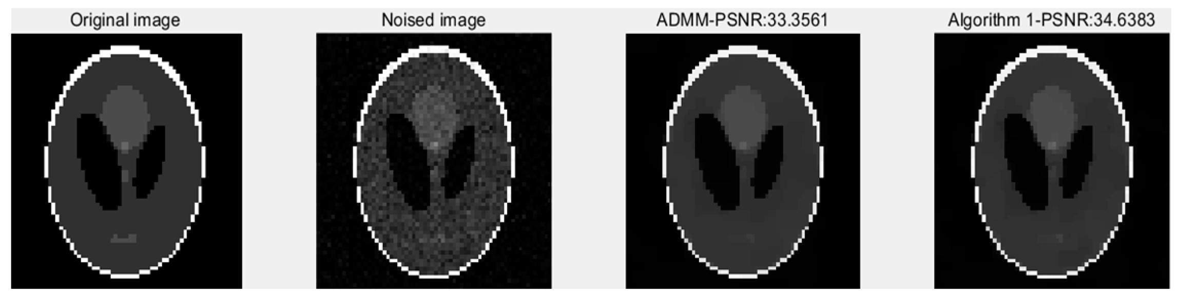
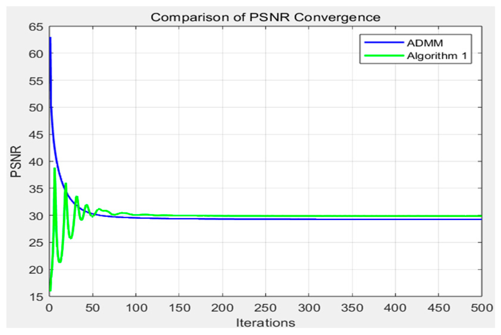
4. Numerical Experiments

This section presents a numerical example to validate the efficacy of Algorithm 1 by addressing the split feasibility problem. The variables and constraints in the experiments exactly match those defined in the theoretical part, thereby ensuring that the experiments can effectively test the validity and practicality of the theory. In the experimental stage, we compare Algorithm 1 with the traditional proximal algorithm to demonstrate how superior the performance of Algorithm 1 is when dealing with the split feasibility problem. All codes were implemented using MATLAB R2021a on a desktop computer with 32 GB of RAM.

In the field of CT image reconstruction, the central objective of inverse problems is to restore an image from noisy CT data. This process can be regarded as the following inverse problem:

$$b=Hx+w$$

(30)

where $b\in {ℝ}^m$ is the observed data, $x\in {ℝ}^n$ is the true (original) underlying image, $w\in {ℝ}^m$ represents the measurement error (Gaussian noise at level ${\displaystyle \frac{1}{200}}{‖b‖}_{\infty }$), and $H\in {ℝ}^{m\times m}$ is the Radon transform in X-Ray computer tomography (CT).

In view of the fact that Equation (30) often exhibits ill-posedness and there are significant difficulties in solving it; in order to ensure the stability of the solutions, we conduct an investigation into the following model:

$${\min }_{x\in \mathcal{C}}F(x)+G(x).$$

(31)

where F(x) is the regularization term dependent on prior knowledge of images, G(x) is the fidelity term and α > 0 is a balancing regularization parameter. In this experiment, we consider $F(x)=\parallel Hx-b{\parallel }^2$ and $G={{\displaystyle \sum }}_{i=1}^n\parallel D_{i}x\parallel$, which is a widely used fidelity term in CT reconstruction. The term Dix indicates the discrete gradient of x at pixel I and the sum $\sum \parallel D_{i}x\parallel$ plays the role of total variation (TV) regularization for x. The operator Di at the pixel horizontal gradient operator and vertical gradient operator. Thus, it is easy to rewrite the model (31) as SFP (1) by setting $C=\left\{x\in {ℝ}^n:G(x)\le r\right\},$$Q=\left\{y\in {ℝ}^n:\parallel y-b{\parallel }_2\le \epsilon \right\}$, and y = Hx. The test image is the 96 × 96 Shepp−Logan phantom, corrupted by Gaussian noise with standard deviation σ = 0.05 (equivalent to ε ≈ 4.8 in the feasibility set Q). The parameters that we used for the trials were as follows: $\beta =1.0,\tau =0.5,$${\theta }_1=0.1,{\theta }_2=0.1$, and α = 0.001. The choice of these parameters was primarily based on empirical tuning and theoretical guarantees to ensure the stability and convergence of the algorithm. The settings of $\beta$ and $\tau$ influence the step size and convergence speed of the algorithm, while ${\theta }_1$ and ${\theta }_2$ control the strength of the inertial effects, which helps accelerate convergence. As a regularization parameter, α balances the fidelity term and the regularization term in image reconstruction, significantly impacting image quality.

Figure 1 shows four images: the original sinogram image, the noised sinogram image, the image reconstructed by ADMM, and the image reconstructed by Algorithm 1. A comprehensive comparison of the reconstructed images in Figure 1 shows that Algorithm 1 yields higher-quality images than ADMM. To evaluate image quality more objectively, we used the peak signal-to-noise ratio (PSNR) as a statistical indicator. A higher PSNR value means better image quality, less noise, and a smaller difference between the processed image and the original one. The results show that the PSNR of the image reconstructed by Algorithm 1 is 34.6383, which has a significant advantage over the 33.3561 obtained by the alternating direction method of multipliers (ADMM).

Figure 1. The recovered sinogram image by two algorithms.

From the relationship between the peak signal-to-noise ratio (PSNR) values and the number of repetitions of the two algorithms presented in Figure 2, it can be clearly observed that the images generated by Algorithm 1 are approaching the original image, and their stability is gradually increasing, eventually achieving convergence to the ideal state. This proves our algorithm is successful.

Figure 2. PSNR value of the reconstructed image using two algorithms.

Note: the presented experiment focuses on a specific CT image reconstruction scenario. Although the results highlight the algorithm’s efficacy in this case, further studies with diverse datasets and problem configurations are necessary to comprehensively evaluate the robustness and generality of PSRTADMM. This constitutes an important direction for future research.

5. Conclusions

In this paper, we put forward a partially symmetric regularized two-step inertial alternating direction method of multipliers to deal with non-convex split feasibility problems. The proposed algorithm innovatively includes an intermediate multiplier update and two-step inertial effects in subproblems. Through theoretical analysis under appropriate assumptions, its global convergence is proven. In addition, when the augmented Lagrangian function satisfies the Kurdyka−Łojasiewicz (KL) property, the algorithm can achieve a strong convergence, which means it can converge to a more accurate solution. Finally, numerical experiments were conducted in the field of CT image reconstruction. The results show that the proposed algorithm outperforms traditional methods in terms of the reconstruction quality and convergence speed, further confirming its effectiveness.

References

- Wang, Y.; Yang, J.; Yin, W.; Zhang, Y. A New Alternating Minimization Algorithm for Total Variation Image Reconstruction. SIAM J. Imaging Sci. 2008, 1, 248–272. [Google Scholar] [CrossRef]
- Dong, B.; Li, J.; Shen, Z. X-Ray CT Image Reconstruction via Wavelet Frame Based Regularization and Radon Domain Inpainting. J. Sci. Comput. 2013, 54, 333–349. [Google Scholar] [CrossRef]
- Block, K.T.; Uecker, M.; Frahm, J. Undersampled radial MRI with multiple coils. Iterative image reconstruction using a total variation constraint. Magn. Reson. Med. 2007, 57, 1086–1098. [Google Scholar] [CrossRef]
- Liu, S.; Cao, J.; Liu, H.; Zhou, X.; Zhang, K.; Li, Z. MRI reconstruction via enhanced group sparsity and nonconvex regularization. Neurocomputing 2018, 272, 108–121. [Google Scholar] [CrossRef]
- Lustig, M.; Donoho, D.; Pauly, J.M. Sparse MRI: The application of compressed sensing for rapid MR imaging. Magn. Reson. Med. 2007, 58, 1182–1195. [Google Scholar] [CrossRef]
- Gibali, A.; Kuefer, K.H.; Suess, P. Successive Linear Programing Approach for Solving the Nonlinear Split Feasibility Problem. J. Nonlinear Convex Anal. 2014, 15, 345–353. [Google Scholar]
- Byrne, C. Iterative oblique projection onto convex sets and the split feasibility problem. Inverse Probl. 2002, 18, 441–453. [Google Scholar] [CrossRef]
- Censor, Y.; Motova, A.; Segal, A. Perturbed projections and subgradient projections for the multiple-sets split feasibility problem. J. Math. Anal. Appl. 2007, 327, 1244–1256. [Google Scholar] [CrossRef]
- Dang, Y.; Gao, Y. The strong convergence of a KM-CQ-like algorithm for a split feasibility problem. Inverse Probl. 2011, 27, 015007. [Google Scholar] [CrossRef]
- Qu, B.; Wang, C.; Xiu, N. Analysis on Newton projection method for the split feasibility problem. Comput. Optim. Appl. 2017, 67, 175–199. [Google Scholar] [CrossRef]
- Fukushima, M. Application of the alternating direction method of multipliers to separable convex programming problems. Comput. Optim. Appl. 1992, 1, 93–111. [Google Scholar] [CrossRef]
- Deng, W.; Yin, W. On the Global and Linear Convergence of the Generalized Alternating Direction Method of Multipliers. J. Sci. Comput. 2016, 66, 889–916. [Google Scholar] [CrossRef]
- Wang, Y.; Yin, W.; Zeng, J. Global Convergence of ADMM in Nonconvex Nonsmooth Optimization. J. Sci. Comput. 2019, 78, 29–63. [Google Scholar] [CrossRef]
- Yang, Y.; Jia, Q.S.; Xu, Z.; Guan, X.; Spanos, C.J. Proximal ADMM for nonconvex and nonsmooth optimization. Automatica 2022, 146, 110551. [Google Scholar] [CrossRef]
- Ouyang, Y.; Chen, Y.; Lan, G.; Pasiliao, E., Jr. An Accelerated Linearized Alternating Direction Method of Multipliers. SIAM J. Imaging Sci. 2015, 8, 644–681. [Google Scholar] [CrossRef]
- Hong, M.; Luo, Z.-Q. On the linear convergence of the alternating direction method of multipliers. Math. Program. 2017, 162, 165–199. [Google Scholar] [CrossRef]
- Zhao, Y.; Li, M.; Pen, X.; Tan, J. Partial symmetric regularized alternating direction method of multipliers for non-convex split feasibility problems. AIMS Math. 2025, 10, 3041–3061. [Google Scholar] [CrossRef]
- Dang, Y.; Chen, L.; Gao, Y. Multi-block relaxed-dual linear inertial ADMM algorithm for nonconvex and nonsmooth problems with nonseparable structures. Numer. Algorithms 2025, 98, 251–285. [Google Scholar] [CrossRef]
- Rockafellar, R.T.; Wets, R.J.-B. Variational Analysis; Springer Science and Business Media: Berlin/Heidelberg, Germany, 2009. [Google Scholar]
- Bolte, J.; Daniilidis, A.; Lewis, A. The Lojasiewicz inequality for nonsmooth subanalytic functions with applications to subgradient dynamical systems. SIAM J. Optim. 2007, 17, 1205–1223. [Google Scholar] [CrossRef]
- Attouch, H.; Bolte, J.; Svaiter, B.F. Convergence of descent methods for semi-algebraic and tame problems: Proximal algorithms, forward–backward splitting, and regularized Gauss–Seidel methods. Math. Program. 2013, 137, 91–129. [Google Scholar] [CrossRef]
- Wang, F.; Cao, W.; Xu, Z. Convergence of multi-block Bregman ADMM for nonconvex composite problems. Sci. China-Inf. Sci. 2018, 61, 122101. [Google Scholar] [CrossRef]
- Nesterov, Y. Introductory Lectures on Convex Optimization: A Basic Course; Springer: New York, NY, USA, 2004. [Google Scholar]
Disclaimer/Publisher’s Note: The statements, opinions and data contained in all publications are solely those of the individual author(s) and contributor(s) and not of MDPI and/or the editor(s). MDPI and/or the editor(s) disclaim responsibility for any injury to people or property resulting from any ideas, methods, instructions or products referred to in the content.  |
© 2025 by the authors. Licensee MDPI, Basel, Switzerland. This article is an open access article distributed under the terms and conditions of the Creative Commons Attribution (CC BY) license (https://creativecommons.org/licenses/by/4.0/).