A Matrix Approach by Convolved Fermat Polynomials for Solving the Fractional Burgers’ Equation

Abstract

This article employs certain polynomials that generalize standard Fermat polynomials, called convolved Fermat polynomials, to numerically solve the fractional Burgers’ equation. New theoretical results of these polynomials are developed and utilized along with the collocation method to find approximate solutions of the fractional Burgers’ equation. The basic idea behind the proposed numerical algorithm is based on establishing the operational matrices of derivatives of both integer and fractional derivatives of the convolved Fermat polynomials that help to convert the equation governed by its underlying conditions into an algebraic system of equations that can be treated numerically. A comprehensive study is performed to analyze the error of the proposed convolved Fermat expansion. Some numerical examples are presented to test our proposed numerical algorithm, and some comparisons are made. The results indicate that the proposed algorithm is applicable and accurate.

1. Introduction

Fractional differential equations (FDEs) have gained interest in science, engineering, and technology because they describe systems with complex and anomalous processes involving infinite correlations. They have applications across many fields of applied sciences, so the investigations for these equations have attracted much interest. Some applications for FDEs can be found in [1,2,3]. Due to the inability to solve these equations analytically, it is important to resort to numerical analysis with different approaches. Many numerical approaches are employed to treat the different types of FDEs. Among these methods are the Adomian decomposition method [4,5], the variational iteration transform method [6], the Laplace transform method [7], the wavelet neural method [8], the Haar wavelets method [9], the generalized Taylor wavelets [10], the Adams–Bashforth–Moulton methods [11,12], the homotopy perturbation method [13], the shifted Gegenbauer–Gauss collocation method [14], the shifted Jacobi collocation method [15], and the localized hybrid kernel meshless method [16].

The classical Burgers’ equation is one of the most essential FDEs; it employs fractional derivatives to describe a wide range of physical events. This equation has been significantly extended to derive the fractional Burgers’ equation. This equation becomes even more critical when modeling processes with typical diffusion or memory effects because traditional integer-order differential equations cannot account for them. Understanding the physical meaning of the fractional Burgers’ equation is crucial. In [17,18], the authors highlighted the role of this equation in modeling subdiffusion convection processes relevant to various physical problems and in describing the propagation of weakly nonlinear acoustic waves through gas-filled pipes, respectively. Many numerical algorithms have been employed to solve the fractional Burgers’ equation. For example, in [19], the time-fractional Burgers’ equation was solved based on the Haar–Sinc spectral approach. Recently, the authors of [20] followed a compact difference tempered fractional Burgers’ equation. A discontinuous Galerkin method was used to treat the time-fractional Burgers’ equation. The homotopy method was applied in [21]. The authors of [22] solved the one- and two-dimensional time-fractional Burgers’ equation using Lucas polynomials. Some other contributions can be found in [23,24,25,26,27].

Modern engineering and physics applications necessitate a more comprehensive understanding of applied mathematics than previously required. Specifically, a solid grasp of the fundamental properties of special functions is essential. These functions are frequently used in various fields, including communication systems, electromagnetic theory, quantum mechanics, approximation theory, probability theory, electrical circuit theory, and heat conduction. For some applications of special functions, one can refer to [28,29].

Fibonacci and Lucas polynomials and their generalizations have been extensively studied in the mathematical literature due to their rich properties and diverse applications across various fields, such as combinatorics, graph theory, and numerical analysis. These polynomials are extensively used in numerical analysis to solve several differential equations (DEs). We give some contributions in this direction. In [30], the author used Fibonacci polynomials to treat FDEs. The authors of [31] treated numerically a modified epidemiological model of computer viruses using Fibonacci wavelets. Pell polynomials were used in [32] to solve stochastic FDEs. Another application for the Pell polynomials was given in [33]. Shifted Lucas polynomials were used in [34] to solve the time-fractional FitzHugh–Nagumo DEs. Other shifted Horadam polynomials were used to solve the nonlinear fifth-order KdV equations in [35]. In [36], the authors treated fractional Bagley–Torvik using Fibonacci wavelets. The authors of [37] handled the Lane–Emden type equation using combined Pell–Lucas polynomials. Vieta–Lucas polynomials were used in [38] to solve specific systems of FDEs using an operational approach.

Among the extensions of Fibonacci sequences are the convolved generalized Fibonacci polynomials, which were presented and examined in [39]. These polynomials extend several classical sequences, including Fibonacci and Pell polynomials and their generalized ones. In [40], the authors examined some features of the convolved generalized Fibonacci and Lucas polynomials. Some other formulas concerned with the convolved polynomials were developed in [41]. In [42], the authors introduced certain generalizations of convolved generalized Fibonacci and Lucas polynomials. In [43], the authors formulated novel formulas for convolved Pell polynomials. In [44], the authors developed some new formulas for convolved Fibonacci polynomials. This paper will introduce and use particular polynomials of the generalized ones introduced in [39], namely, convolved Fermat polynomials. These polynomials generalize the standard conventional Fermat polynomials.

Spectral methods are a class of numerical methods that approximate the solution of differential equations by expanding the solution in terms of global basis functions, which are typically special functions. In contrast to finite difference and finite element methods, spectral methods use global approximations. A key advantage of spectral methods is their exponential convergence to solutions in smooth scenarios; that is, the error decays fast as the basis functions count increases. This means that spectral methods are ideal for highly accurate models. There are three major categories of spectral methods. These are the Galerkin, tau, and collocation methods. With the spectral Galerkin method, the solution is written as a series of basis functions, and the residual is ensured to be orthogonal to these functions. In addition, the selected trial and test functions should coincide. In [45], the authors handled some partial DEs through the Galerkin method. In [46], the authors applied spectral Galerkin methods for some FDEs. The authors of [47] used the Galerkin method and generalized Chebyshev polynomials to treat some fractional delay pantograph DEs. The tau method is unlike the Galerkin method in that one is free to pick the trial and test functions. The authors of [48] utilized the tau method to treat the time-fractional cable problem. In [49], the authors treated systems of fractional-order integro-DEs using the tau method along with the monic Laguerre polynomial. Other integro-DEs were treated in [50] using a tau–Gegenbauer spectral method. In the collocation method, the residual should vanish at some discrete collocation points. This approach is advantageous due to its applicability to all types of DEs, so it is used extensively to treat many DEs. For example, the authors of [51] followed a collocation approach to certain stochastic FDEs. Another collocation method based on Chebyshev polynomials was used in [52] to solve some elliptic partial DEs. In [53], the Laguerre spectral collocation method was used to solve the space-fractional diffusion equation. The authors of [54] followed a collocation method to treat FitzHugh-–Nagumo DEs. Another collocation method was employed in [55] to treat certain variable-order FDEs.

This paper concentrates on the numerical solution of the time-fractional Burgers’ equation [56]:

$${\displaystyle \frac{{\partial }^{\beta }\chi (\sigma ,t)}{\partial t^{\beta }}}+\chi (\sigma ,t){\displaystyle \frac{\partial \chi (\sigma ,t)}{\partial \sigma }}-\mathsf{\Psi }{\displaystyle \frac{{\partial }^2\chi (\sigma ,t)}{\partial {\sigma }^2}}=G(\sigma ,t),0<\beta <1,$$

(1)

with the following conditions:

$$\begin{array}{cc}\hfill \chi (\sigma ,0)=& {\chi }_1\left(\sigma \right),0<\sigma \le 1,\hfill \end{array}$$

(2)

$$\begin{array}{cc}\hfill \chi (0,t)=& {\chi }_2\left(t\right),\chi (1,t)={\chi }_3\left(t\right),0<t\le 1,\hfill \end{array}$$

(3)

where $G(\sigma ,t)$ represents the source term and $\mathsf{\Psi }$ represents the kinematic viscosity.

We comment here on the remark of Wang and He in  [57], in which they demonstrated that, to maintain consistency, both time and space are modeled fractionally—a principle termed the fractional spatio-temporal relation. This generalization will be a target for us in a forthcoming paper.

The following are the primary objectives of this paper:

• Providing certain polynomials that generalize the well-known standard Fermat polynomials, called the convolved Fermat polynomials.
• Establishing the analytic and inversion formulas of these polynomials.
• Constructing the operational derivative matrices of the convolved Fermat polynomials for both integer and fractional derivatives.
• Developing a collocation technique to handle the time-fractional Burgers’ equation.
• Analyzing the convergence and error analysis of the convolved Fermat expansion.
• Testing the accuracy of our numerical algorithm against other established techniques to demonstrate its effectiveness.

Furthermore, we mention here that some advantages and original contributions in this work can be listed as follows:

• The new theoretical results concerning the convolved Fermat polynomials are new. We think that the theoretical background of these polynomials in this paper may be utilized in other contributions in the scope of the numerical solutions of differential equations.
• To our knowledge, employing such polynomials in numerical analysis is new. This gives us motivation for our study.
• Highly accurate solutions can be obtained by employing the convolved Fibonacci polynomials as basis functions.

The rest of the paper is organized as follows. The next section overviews the convolved generalized polynomials and some of their particular polynomials. Some new formulas of the convolved Fermat polynomials, such as their power form representation and its inversion formula, are developed in Section 3. Section 4 analyzes the numerical algorithm designed to solve the fractional Burgers’ equation based on the application of the collocation method using the convolved Fermat polynomials as basis functions. The convergence of the convolved Fermat expansion is presented in Section 5 by stating and proving some lemmas and theorems. Some illustrative examples are presented in Section 6 accompanied by comparisons with some other algorithms to test our numerical algorithm. Finally, Section 7 presents the concluding findings.

2. Fundamentals and Essential Relations

This section is confined to introducing an account of some essential characteristics of fractional calculus, the generalized convolved polynomials, and some of their particular polynomials.

2.1. Caputo’s Fractional Derivative

Definition 1

([58]). In the Caputo sense, the fractional derivative $D_s^{\beta }\xi \left(s\right)$ is defined as

$${\displaystyle D_s^{\beta }\xi \left(s\right)=\frac{1}{\mathsf{\Gamma }(r-\beta )}{\int }_0^s{(s-t)}^{r-\beta -1}{\xi }^{\left(r\right)}\left(t\right)dt,\beta >0,s>0,r-1<\beta \le r,r\in \mathbb{N}.}$$

(4)

For $D_s^{\beta }$ with $r-1<\beta \le r,r\in \mathbb{N}$, the following identities are valid:

$$\begin{array}{cc}\hfill D_s^{\beta }C=& 0,C\mathrm{is}\mathrm{a}\mathrm{constant},\hfill \end{array}$$

(5)

$$\begin{array}{cc}\hfill D_s^{\beta }{s}^r=& \left\{\begin{array}{cc}0,\hfill & \mathrm{if} r\in {\mathbb{N}}_{0}andr<\lceil \beta \rceil ,\hfill \\ {\displaystyle \frac{r!}{\mathsf{\Gamma }(r-\beta +1)}}{s}^{r-\beta },\hfill & \mathrm{if} r\in {\mathbb{N}}_{0}andr\ge \lceil \beta \rceil ,\hfill \end{array}\right.\hfill \end{array}$$

(6)

where $\mathbb{N}=\{1,2,\dots \}$  and  ${\mathbb{N}}_0=\{0,1,2,\dots \}$, and $\lceil \beta \rceil$ is the ceiling function.

Remark 1.

For some other definitions of fractional derivatives and their applications, one can refer to [59,60].

2.2. An Account on Fermat Polynomials

If we consider the first kind of the Lucas polynomial sequence ${\left\{{\varphi }_i^{a,b}\left(t\right)\right\}}_{i\ge 0}$ generated by the recursive formula [39]:

$${\psi }_i^{a,b}\left(t\right)=at{\psi }_{i-1}^{a,b}\left(t\right)+b{\psi }_{i-2}^{a,b}\left(t\right),{\psi }_0^{a,b}\left(t\right)=1,{\psi }_1^{a,b}\left(t\right)=at,$$

(7)

then the Fermat polynomials are particular cases of ${\psi }_i^{a,b}\left(t\right)$ corresponding to $a=3,b=-2$. Thus, the sequence ${\left\{{\mathcal{F}}_k\left(t\right)\right\}}_{k\ge 0}$ may be constructed using the following recursive formula:

$${\mathcal{F}}_k\left(t\right)=3t{\mathcal{F}}_{k-1}\left(t\right)+2{\mathcal{F}}_{k-2}\left(t\right).$$

(8)

These polynomials are explicitly expressed by the following formula [61]:

$${\mathcal{F}}_k\left(t\right)=\sum _{r=0}^{⌊{\displaystyle \frac{k}{2}}⌋}{3}^{k-2r}{(-2)}^r\left({\displaystyle \genfrac{}{}{0pt}{}{k-r}{r}}\right)t^{k-2r},$$

(9)

and their inversion formula is given by [61]

$$t^k=\sum _{r=0}^{⌊{\displaystyle \frac{k}{2}}⌋}{\displaystyle \frac{{(-1)}^r(k-2r+1){(k-r+2)}_{r-1}{(-2)}^r}{r!3^k}}{\mathcal{F}}_{k-2r}\left(t\right).$$

(10)

2.3. Convolved Generalized Fibonacci Polynomials

In [39], the authors developed the convolved generalized Fibonacci polynomials, denoted as ${\mathcal{CGF}}_j^{r,s,\mu }\left(\sigma \right)$, where $r=r\left(\sigma \right)$ and $s=s\left(\sigma \right)$ are polynomials with real coefficients, and $\mu$ is a complex integer. The generating function for ${\mathcal{CGF}}_j^{r,s,\mu }\left(\sigma \right)$ is [39]

$${\displaystyle {\left(1-r\left(\sigma \right)t-s\left(\sigma \right)t^2\right)}^{-\mu }=\sum _{k=0}^{\infty }{\mathcal{CGF}}_k^{r,s,\mu }\left(\sigma \right)t^k.}$$

Furthermore, they can be represented as

$${\displaystyle {\mathcal{CGF}}_k^{r,s,\mu }\left(\sigma \right)=\sum _{r=0}^{⌊\frac{k}{2}⌋}\left(\genfrac{}{}{0pt}{}{\mu +r-1}{r}\right)\left(\genfrac{}{}{0pt}{}{\mu +k-r-1}{k-2r}\right)r^{k-2r}\left(\sigma \right)s^r\left(\sigma \right),}$$

(11)

and they can be generated with the aid of the following recursive formula [39]:

$$k{\mathcal{CGF}}_k^{r,s,\mu }\left(\sigma \right)-(\mu +k-1)r\left(\sigma \right){\mathcal{CGF}}_{k-1}^{r,s,\mu }\left(\sigma \right)-(2\mu +k-2)s\left(\sigma \right){\mathcal{CGF}}_{k-2}^{r,s,\mu }\left(\sigma \right)=0,k\ge 2,$$

(12)

with the following initial values:

$${\mathcal{CGF}}_0^{r,s,\mu }\left(\sigma \right)=1,{\mathcal{CGF}}_1^{r,s,\mu }\left(\sigma \right)=\mu r\left(\sigma \right).$$

Remark 2.

Many celebrated sequences can be extracted as particular sequences of the convolved generalized Fibonacci polynomials. Among these sequences are the following sequences:

• The convolved Fibonacci polynomials ${\mathcal{CF}}_k\left(\sigma \right)$, which were investigated theoretically in [44] and employed numerically in [62]. These polynomials are defined as

  $${\mathcal{CF}}_k\left(\sigma \right)={\mathcal{CGF}}_k^{\sigma ,1,\mu }\left(\sigma \right).$$
• The convolved Pell polynomials ${\mathcal{CP}}_k\left(\sigma \right)$, which were investigated theoretically in [62]. These polynomials are defined as

  $${\mathcal{CP}}_k\left(\sigma \right)={\mathcal{CGF}}_k^{2\sigma ,1,\mu }\left(\sigma \right).$$

2.4. Convolved Fermat Polynomials

This paper introduces a sequence of polynomials that generalize the Fermat sequence of polynomials, called convolved Fermat polynomials. These polynomials are particular polynomials of the polynomials generated by (12). More precisely, they can be obtained from the polynomials ${\mathcal{CGF}}_k^{r,s,\mu }\left(x\right)$ with the following choices:

$$r\left(\sigma \right)=3\sigma ,s\left(\sigma \right)=-2,\mu =n,$$

where n is a positive real constant.

We will denote these polynomials by ${\varphi }_i^n\left(\sigma \right)$. The recursive formula fulfilled by ${\varphi }_i^n\left(\sigma \right)$ is

$$2(i+2n-2){\varphi }_{i-2}^n\left(\sigma \right)-3\sigma (i+n-1){\varphi }_{i-1}^n\left(\sigma \right)+i{\varphi }_i^n\left(\sigma \right)=0,i\ge 2.$$

(13)

Form (11), the analytic form of the convolved Fermat polynomials, ${\varphi }_i^n\left(\sigma \right)$ takes the following form:

$${\varphi }_i^n\left(\sigma \right)=\sum _{r=0}^{⌊{\displaystyle \frac{i}{2}}⌋}{\displaystyle \frac{{(-2)}^r{3}^{i-2r}{\left(n\right)}_{i-r}}{r!(i-2r)!}}{\sigma }^{i-2r}.$$

(14)

Remark 3.

It is useful to write the power form representation (14) in the following alternative form:

$${\varphi }_i^n\left(\sigma \right)=\sum _{k=0}^i{\displaystyle \frac{3^k{(-2)}^{\frac{i-k}{2}}{a}_{i+k}{\left(n\right)}_{\frac{i+k}{2}}}{k!\left(\frac{i-k}{2}\right)!}}{\sigma }^k,$$

(15)

$$a_r=\left\{\begin{array}{cc}1,\hfill & ifr\mathit{even},\hfill \\ 0,\hfill & otherwise.\hfill \end{array}\right.$$

(16)

Remark 4.

Fermat polynomials ${\mathcal{FR}}_k$ generated by (8) are particular polynomials of the convolved Fermat polynomials in the sense that

$${\mathcal{FR}}_k\left(\sigma \right)={\varphi }_k^1\left(\sigma \right).$$

The next section develops some new formulas regarding the convolved Fermat polynomials that will be useful in the sequel.

3. Some New Formulas of the Convolved Fermat Polynomials

Our suggested numerical technique for solving the fractional Burger’s equation relies heavily on some new formulas of the convolved Fermat polynomials, which are the focus of this section. Our focus will be to develop the following formulas:

• The inversion formula of the convolved Fermat polynomials.
• An explicit formula for the integer and fractional derivatives of the convolved Fermat polynomials.
• The operational matrices of the integer derivatives of the convolved Fermat polynomials.
• An explicit formula for the fractional derivatives of the convolved Fermat polynomials.
• The operational matrices of both integer and fractional derivatives of the convolved Fermat polynomials.

The following theorem displays the inversion formula for the power Formula (14). First, one requires the lemma below.

Lemma 1.

Consider p to be any non-negative integer. The following identity is valid:

$$\sum _{m=0}^p{\displaystyle \frac{{(-1)}^m(i-2m+n)(i-m+n-p-1)!}{m!(i-m+n)!(i-2p)!(p-m)!}}=\left\{\begin{array}{cc}{\displaystyle \frac{1}{i!}},\hfill & p=0,\hfill \\ 0,\hfill & p>0.\hfill \end{array}\right.$$

(17)

Proof. 

It is clear that the identity holds for $p=0$, so to complete the proof we set

$$S_{p,i}=\sum _{m=0}^p{\displaystyle \frac{{(-1)}^m(i-2m+n)(i-m+n-p-1)!}{m!(i-m+n)!(i-2p)!(p-m)!}},p\ge 1.$$

and we will show that

$$S_{p,i}=0,p\ge 1.$$

We can write $S_{p,i}$ as

$$\begin{array}{cc}\hfill S_{p,i}=& \sum _{m=1}^{p+1}{\displaystyle \frac{{(-1)}^{m+1}(2+i-2m+n)(i-m+n-p)!}{(m-1)!(1+i-m+n)!(i-2p)!(1-m+p)!}}\hfill \\ \hfill =& \sum _{m=1}^p{\displaystyle \frac{{(-1)}^{m+1}(2+i-2m+n)(i-m+n-p)!}{(m-1)!(1+i-m+n)!(i-2p)!(1-m+p)!}}+{\displaystyle \frac{{(-1)}^p(i+n-2p)!}{(i-2p)!(i+n-p)!p!}}.\hfill \end{array}$$

We write the last formula in the form

$$S_{p,i}=M_{p,i}+{\displaystyle \frac{{(-1)}^p(i+n-2p)!}{(i-2p)!(i+n-p)!p!}},$$

(18)

with

$$M_{p,i}=\sum _{m=1}^p{\displaystyle \frac{{(-1)}^{m+1}(2+i-2m+n)(i-m+n-p)!}{(m-1)!(1+i-m+n)!(i-2p)!(1-m+p)!}}.$$

Now, Zeilberger’s algorithm [63] aids in finding a closed form for $M_{p,i}$. The recurrence relation that satisfied by $M_{p,i}$ is

$$\begin{array}{cc}\hfill & (p+1)(-2p+i+n-1)(-2p+i+n)M_{p+1,i}\hfill \\ \hfill & +(-2p+i-1)(-2p+i)(-p+i+n)M_{p,i}=0,\hfill \end{array}$$

(19)

with the initial condition

$$M_{0,i}={\displaystyle \frac{(i+n)(-2+i+n)!}{(-2+i)!(i+n)!}}.$$

The exact solution of (19) is given by

$$M_{p,i}={\displaystyle \frac{{(-1)}^{p+1}(i+n-2p)!}{(i-2p)!(i+n-p)!p!}}.$$

(20)

The closed form in (20) together with Formula (18) implies that

$$S_{p,i}=0,p\ge 1.$$

This ends the proof.    □

Theorem 1.

Let i be any real non-positive integer. The inversion formula of ${\varphi }_i^n\left(\sigma \right)$ is given by

$${\sigma }^i={\displaystyle \frac{i!}{3^i}}\sum _{r=0}^{⌊{\displaystyle \frac{i}{2}}⌋}{\displaystyle \frac{2^r}{r!{\left(n\right)}_{i-2r}{(i+n-2r+1)}_r}}{\varphi }_{i-2r}^n\left(\sigma \right).$$

(21)

Proof. 

To prove Formula (21), we consider

$$Z\left(\sigma \right)={\displaystyle \frac{i!}{3^i}}\sum _{r=0}^{⌊{\displaystyle \frac{i}{2}}⌋}{\displaystyle \frac{2^r}{r!{\left(n\right)}_{i-2r}{(i+n-2r+1)}_r}}{\varphi }_{i-2r}^n\left(\sigma \right),$$

and we will show that

$$Z\left(\sigma \right)={\sigma }^i.$$

Now, based on the analytic form in (14), $Z\left(\sigma \right)$ can be written as

$$\begin{array}{cc}\hfill Z\left(\sigma \right)=& 3^{-i}i!\sum _{m=0}^{⌊{\displaystyle \frac{i}{2}}⌋}{\displaystyle \frac{2^m}{m!{\left(n\right)}_{i-2m}{(1+i-2m+n)}_m}}\times \hfill \\ \hfill & \sum _{r=0}^{⌊{\displaystyle \frac{i}{2}}⌋-m}{\displaystyle \frac{{(-2)}^r{3}^{i-2m-2r}{\left(n\right)}_{i-2m-r}}{(i-2m-2r)!r!}}{\sigma }^{i-2m-2r},\hfill \end{array}$$

(22)

which can be represented as

$$\begin{array}{c}\hfill Z\left(\sigma \right)=\sum _{p=0}^{⌊{\displaystyle \frac{i}{2}}⌋}{\left(-{\displaystyle \frac{2}{9}}\right)}^{p}i!{\sigma }^{i-2p}\sum _{m=0}^p{\displaystyle \frac{{(-1)}^m(i-2m+n)(i-m+n-p-1)!}{m!(i-m+n)!(i-2p)!(p-m)!}},\end{array}$$

(23)

which is also equivalent to

$$\begin{array}{c}\hfill Z\left(\sigma \right)={\sigma }^i+\sum _{p=1}^{⌊{\displaystyle \frac{i}{2}}⌋}{\left(-{\displaystyle \frac{2}{9}}\right)}^{p}i!{\sigma }^{i-2p}\sum _{m=0}^p{\displaystyle \frac{{(-1)}^m(i-2m+n)(i-m+n-p-1)!}{m!(i-m+n)!(i-2p)!(p-m)!}}.\end{array}$$

(24)

It is clear now that the application of Lemma 1 leads to

$$Z\left(\sigma \right)={\sigma }^i,$$

and, accordingly, the proof is now complete.    □

Remark 5.

Equation (21) can be rewritten in another form as

$${\sigma }^p=\sum _{L=0}^p{H}_{L,p}{\varphi }_L^n\left(\sigma \right),$$

(25)

where

$$H_{r,i}={\displaystyle \frac{i!2^{\frac{i-r}{2}}{a}_{i+r}}{3^i\left(\frac{i-r}{2}\right)!{\left(n\right)}_r{(n+r+1)}_{\frac{i-r}{2}}}}.$$

(26)

Theorem 2.

For any positive integers q and i with $i\ge q$, the qth-derivative of ${\varphi }_i^n\left(\sigma \right)$ can be expressed as

$${\displaystyle \frac{d^q{\varphi }_i^n\left(\sigma \right)}{d{\sigma }^q}}=\sum _{k=0}^{i-q}{\mathcal{A}}_{i,k}^q{\varphi }_k^n\left(\sigma \right),$$

(27)

where

$$\begin{array}{cc}\hfill {\mathcal{A}}_{i,k}^q=& 3^q{(-1)}^{i-k-q}{2}^{{\displaystyle \frac{1}{2}}(i-k-q)}(k+n)\left({\displaystyle \genfrac{}{}{0pt}{}{\frac{1}{2}(i-k+q-2)}{\frac{1}{2}(i-k-q)}}\right)\times \hfill \\ \hfill & {\left({\displaystyle \frac{1}{2}}(2+i+k+2n-q)\right)}_{q-1}{a}_{i-k-q},\hfill \end{array}$$

(28)

and $a_k$ is defined as in (16).

Proof. 

Differentiating Formula (14) q times with respect to $\sigma$ yields

$$D^q{\varphi }_i^n\left(\sigma \right)=\sum _{j=0}^{⌊{\displaystyle \frac{i-q}{2}}⌋}{\displaystyle \frac{{(-2)}^j{3}^{i-2j}{\left(n\right)}_{i-j}{(1+i-2j-q)}_q}{(i-2j)!j!}}{\sigma }^{i-2j-q}.$$

(29)

The application of the inversion Formula (21) leads to the following formula:

$$\begin{array}{cc}\hfill D^q{\varphi }_i^n\left(\sigma \right)=& {\displaystyle \frac{3^q}{(n-1)!}}\sum _{j=0}^{⌊{\displaystyle \frac{i-q}{2}}⌋}{\displaystyle \frac{{(-2)}^j(i-j+n-1)!}{j!}}\times \hfill \\ \hfill & \sum _{r=0}^{⌊{\displaystyle \frac{i-q}{2}}⌋-j}{\displaystyle \frac{2^r}{r!{\left(n\right)}_{i-2j-q-2r}{(1+i-2j+n-q-2r)}_r}}{\varphi }_{i-q-2(j+r)}^n\left(\sigma \right),\hfill \end{array}$$

(30)

which can be written alternatively as

$$\begin{array}{c}\hfill D^q{\varphi }_i^n\left(\sigma \right)=\sum _{L=0}^{⌊{\displaystyle \frac{i-q}{2}}⌋}{(-2)}^L(i-2L+n-q)\sum _{s=0}^L{\displaystyle \frac{{(-1)}^{L-s}{3}^q(i+n-s-1)!}{s!(L-s)!(i-L+n-q-s)!}}{\varphi }_{i-q-2L}^n\left(\sigma \right),\end{array}$$

(31)

which can be expressed again as

$$\begin{array}{cc}\hfill D^q{\varphi }_i^n\left(\sigma \right)& =3^q(i+n-1)!\sum _{L=0}^{⌊{\displaystyle \frac{i-q}{2}}⌋}{\displaystyle \frac{{(-1)}^{L+1}(-i+2L-n+q){(-2)}^L}{L!(i-L+n-q)!}}\times \hfill \\ \hfill & {}_{2}F_1\left(\begin{array}{c}-L,-i+L-n+q\\ 1-i-n\end{array}{\displaystyle |}1\right){\varphi }_{i-q-2L}^n\left(\sigma \right).\hfill \end{array}$$

(32)

Using Chu Vandermond’s identity [64], the above ${}_{2}F_1\left(1\right),$ can be summed to give the following closed form:

$${}_{2}F_1\left(\begin{array}{c}-L,-i+L-n+q\\ 1-i-n\end{array}|1\right)={\displaystyle \frac{(i-L+n-1)!(L+q-1)!}{(i+n-1)!(q-1)!}},$$

and, accordingly, Formula (32) turns into

$$\begin{array}{cc}\hfill D^q{\varphi }_i^n\left(\sigma \right)=& 3^q\sum _{L=0}^{⌊{\displaystyle \frac{i-q}{2}}⌋}{(-1)}^L(i-2L+n-q){(-2)}^L\left({\displaystyle \genfrac{}{}{0pt}{}{-1+L+q}{L}}\right){(i-L+n+1-q)}_{q-1}\times \hfill \\ \hfill & {\varphi }_{i-q-2L}^n\left(\sigma \right).\hfill \end{array}$$

(33)

The last formula can be written as in (27). This proves Theorem 2.    □

Corollary 1.

${\displaystyle \frac{d{\varphi }_i^n\left(\sigma \right)}{d\sigma }}$ has the form

$${\displaystyle \frac{d{\varphi }_i^n\left(\sigma \right)}{d\sigma }}=\sum _{k=0}^{i-1}{\lambda }_{k,i}{\varphi }_k^n\left(\sigma \right),i\ge 1,$$

(34)

where

$${\lambda }_{k,i}=3{(-1)}^{i-k+1}{2}^{\frac{1}{2}(i-k-1)}(k+n)a_{i-k-1}.$$

(35)

Proof. 

Formula (34) may be readily obtained by substituting $q=1$ in Theorem 2.    □

Corollary 2.

${\displaystyle \frac{d^2{\varphi }_i^n\left(\sigma \right)}{d{\sigma }^2}}$ has the form

$${\displaystyle \frac{d^2{\varphi }_i^n\left(\sigma \right)}{d{\sigma }^2}}=\sum _{k=0}^{i-2}{\gamma }_{k,i}{\varphi }_k^n\left(\sigma \right),i\ge 2,$$

(36)

where

$${\gamma }_{k,i}=9{(-1)}^{i-k}{2}^{\frac{1}{2}(i-k-6)}(i-k)(k+n)(i+k+2n)a_{i-k}.$$

(37)

Proof. 

Formula (36) may be readily obtained by substituting $q=2$ in Theorem 2.    □

Remark 6.

As immediate consequences of Corollaries 1 and 2, the operational matrices of derivatives of the convolved Fermat polynomials can be deduced. The following corollary presents this result.

Corollary 3.

If we define the vector ${\mathit{\varphi }}^n\left(\sigma \right)={[{\varphi }_0^n\left(\sigma \right),{\varphi }_1^n\left(\sigma \right),\dots ,{\varphi }_M^n\left(\sigma \right)]}^T$, then ${\displaystyle \frac{d{\mathit{\varphi }}^n\left(\sigma \right)}{d\sigma }}$, and ${\displaystyle \frac{d^2{\mathit{\varphi }}^n\left(\sigma \right)}{d^2\sigma }}$ can be expressed in the following forms:

$$\begin{array}{cc}\hfill & {\displaystyle \frac{d{\mathit{\varphi }}^n\left(\sigma \right)}{d\sigma }}=\overline{\mathit{\lambda }}{\mathit{\varphi }}^n\left(\sigma \right),\hfill \end{array}$$

(38)

$$\begin{array}{cc}\hfill & {\displaystyle \frac{d^2{\mathit{\varphi }}^n\left(\sigma \right)}{d^2\sigma }}=\overline{\mathit{\gamma }}{\mathit{\varphi }}^n\left(\sigma \right),\hfill \end{array}$$

(39)

where $\overline{\mathit{\lambda }}=\left({\overline{\lambda }}_{k,i}\right)$ and $\overline{\mathit{\gamma }}=\left({\overline{\gamma }}_{k,i}\right)$ are the operational matrices of derivatives of order $(\mathcal{M}+1)\times (\mathcal{M}+1)$ whose entries are, respectively, given as

$$\begin{array}{cc}& {\overline{\lambda }}_{k,i}=\left\{\begin{array}{cc}{\lambda }_{k,i},\hfill & if i>k,\hfill \\ 0,\hfill & otherwise,\hfill \end{array}\right.\hfill \\ & {\overline{\gamma }}_{k,i}=\left\{\begin{array}{cc}{\gamma }_{k,i},\hfill & if i>k+1,\hfill \\ 0,\hfill & otherwise.\hfill \end{array}\right.\hfill \end{array}$$

(40)

For example, the matrices $\overline{\mathit{\lambda }}$ and $\overline{\mathit{\gamma }}$ take the following forms for $\mathcal{M}=6.$

$$\begin{array}{c}\overline{\mathit{\lambda }}=\left(\begin{array}{ccccccc}0& 0& 0& 0& 0& 0& 0\\ 3n& 0& 0& 0& 0& 0& 0\\ 0& 3(n+1)& 0& 0& 0& 0& 0\\ 6n& 0& 3(n+2)& 0& 0& 0& 0\\ 0& 6(n+1)& 0& 3(n+3)& 0& 0& 0\\ 12n& 0& 6(n+2)& 0& 3(n+4)& 0& 0\\ 0& 12(n+1)& 0& 6(n+3)& 0& 3(n+5)& 0\end{array}\right),\hfill \end{array}$$

(41)

$$\begin{array}{cc}\hfill & \overline{\mathit{\gamma }}=\left(\begin{array}{ccccccc}0& 0& 0& 0& 0& 0& 0\\ 0& 0& 0& 0& 0& 0& 0\\ 9n(n+1)& 0& 0& 0& 0& 0& 0\\ 0& 9(n+1)(n+2)& 0& 0& 0& 0& 0\\ 36n(n+2)& 0& 9(n+2)(n+3)& 0& 0& 0& 0\\ 0& 36(n+1)(n+3)& 0& 9(n+3)(n+4)& 0& 0& 0\\ 108n(n+3)& 0& 36(n+2)(n+4)& 0& 9(n+4)(n+5)& 0& 0\end{array}\right).\hfill \end{array}$$

(42)

Theorem 3.

For $0<\beta <1$, the fractional derivative of ${\varphi }_j^n\left(t\right)$ can be represented as

$$D_t^{\beta }{\varphi }_j^n\left(t\right)=t^{-\beta }\left(\sum _{p=0}^j{\psi }_{p,j}^{\beta }{\varphi }_p^n\left(t\right)-{\nu }_j\right),$$

(43)

where

$${\psi }_{p,j}^{\beta }=\sum _{L=p}^j{\displaystyle \frac{L!B_{L,j}{H}_{p,L}}{\mathsf{\Gamma }(L-\beta +1)}},$$

(44)

and

$${\nu }_j={\displaystyle \frac{{(-1)}^{\frac{j}{2}}{2}^{\frac{j}{2}}{a}_j{\left(n\right)}_{\frac{j}{2}}}{\frac{j}{2}!\mathsf{\Gamma }(1-\beta )}}.$$

(45)

Proof. 

Formula (15) allows one to write $D_t^{\beta }{\varphi }_j^n\left(t\right)$ as

$$D_t^{\beta }{\varphi }_j^n\left(t\right)=\sum _{p=1}^j{\displaystyle \frac{p!B_{p,j}}{\mathsf{\Gamma }(p-\beta +1)}}{t}^{p-\beta },$$

(46)

where

$$B_{k,i}={\displaystyle \frac{3^k{(-2)}^{\frac{i-k}{2}}{a}_{i+k}{\left(n\right)}_{\frac{i+k}{2}}}{k!\left(\frac{i-k}{2}\right)!}}.$$

(47)

Now, the inversion Formula (25) can be rewritten as

$$t^p=\sum _{L=0}^p{H}_{L,p}{\varphi }_L^n\left(t\right),$$

(48)

where $H_{L,p}$ is defined in Equation (26). Therefore, we can write Equation (46) after using Equation (48) as

$$D_t^{\beta }{\varphi }_j^n\left(t\right)=t^{-\beta }\sum _{p=1}^j\sum _{L=0}^p{\displaystyle \frac{p!B_{p,j}{H}_{L,p}}{\mathsf{\Gamma }(p-\beta +1)}}{\varphi }_L^n\left(t\right),$$

(49)

which can be transformed into

$$D_t^{\beta }{\varphi }_j^n\left(t\right)=t^{-\beta }\left(\sum _{p=0}^j{\psi }_{p,j}^{\beta }{\varphi }_p^n\left(t\right)-{\nu }_j\right),$$

(50)

where

$${\psi }_{p,j}^{\beta }=\sum _{L=p}^j{\displaystyle \frac{L!B_{L,j}{H}_{p,L}}{\mathsf{\Gamma }(L-\beta +1)}},$$

(51)

and

$${\nu }_j={\displaystyle \frac{{(-1)}^{\frac{j}{2}}{2}^{\frac{j}{2}}{a}_j{\left(n\right)}_{\frac{j}{2}}}{\left(\frac{j}{2}\right)!\mathsf{\Gamma }(1-\beta )}}. \square$$

(52)

Corollary 4.

The fractional derivative of ${\mathit{\varphi }}^{\mathit{n}}\left(t\right)$ can be written in matrix form as

$$D_t^{\beta }{\mathit{\varphi }}^{\mathit{n}}\left(\mathit{t}\right)=t^{-\beta }(\mathit{\psi }{\mathit{\varphi }}^{\mathit{n}}\left(t\right)-\mathit{\nu }),$$

(53)

where $\mathit{\nu }={[{\nu }_0,{\nu }_1,\dots ,{\nu }_{\mathcal{M}}]}^T$. Additionally, $\mathit{\psi }=\left({\psi }_{p,j}^{\beta }\right)$ is the operational matrix of the fractional derivative of order $(\mathcal{M}+1)\times (\mathcal{M}+1)$ whose entries are given, respectively, in (44) and (45).

4. Numerical Technique for the Time-Fractional Burgers’ Equation

This section focuses on presenting a numerical algorithm for solving the time-fractional Burgers’ Equation (1) governed by the initial and boundary conditions (2)–(3).

One may set

$${\mathcal{I}}^{\mathcal{M}}\left(\mathsf{\Omega }\right)=\mathrm{span}\{{\varphi }_i^n\left(\sigma \right){\varphi }_j^n\left(t\right):0\le i,j\le \mathcal{M}\},$$

where $\mathsf{\Omega }=(0,1)\times (0,1)$, and ${\varphi }_i^n\left(\sigma \right)$ are the convolved Fermat polynomials given explicitly in (14).

Consequently, any function ${\chi }^{\mathcal{M}}(\sigma ,t)\in {\mathcal{I}}^{\mathcal{M}}\left(\mathsf{\Omega }\right)$ can be represented as

$${\chi }^{\mathcal{M}}(\sigma ,t)=\sum _{i=0}^{\mathcal{M}}\sum _{j=0}^{\mathcal{M}}{c}_{ij}{\varphi }_i^n\left(\sigma \right){\varphi }_j^n\left(t\right)={\mathit{\varphi }}^{\mathit{n}}{\left(\sigma \right)}^T\mathit{C}{\mathit{\varphi }}^{\mathit{n}}\left(t\right),$$

(54)

where, ${\mathit{\varphi }}^{\mathit{n}}\left(\sigma \right)={[{\varphi }_0^n\left(\sigma \right),{\varphi }_1^n\left(\sigma \right),\dots ,{\varphi }_{\mathcal{M}}^n\left(\sigma \right)]}^T,{\mathit{\varphi }}^{\mathit{n}}\left(t\right)={[{\varphi }_0^n\left(t\right),{\varphi }_1^n\left(t\right),\dots ,{\varphi }_{\mathcal{M}}^n\left(t\right)]}^T,$ and $\mathit{C}={\left(c_{ij}\right)}_{0\le i,j\le \mathcal{M}}$ is the unknown matrix whose order is ${(\mathcal{M}+1)}^2$.

Now, the residual $\mathbf{R}(\sigma ,t)$ of Equation (1) may be expressed as

$$\begin{array}{cc}\hfill \mathbf{R}(\sigma ,t)& ={\displaystyle \frac{{\partial }^{\beta }{\chi }^{\mathcal{M}}(\sigma ,t)}{\partial t^{\beta }}}+{\chi }^{\mathcal{M}}(\sigma ,t){\displaystyle \frac{\partial {\chi }^{\mathcal{M}}(\sigma ,t)}{\partial \sigma }}-\mathsf{\Psi }{\displaystyle \frac{{\partial }^2{\chi }^{\mathcal{M}}(\sigma ,t)}{\partial {\sigma }^2}}-S(\sigma ,t)\hfill \\ & =\sum _{i=0}^{\mathcal{M}}\sum _{j=0}^{\mathcal{M}}{c}_{ij}{\varphi }_i^n\left(\sigma \right){\displaystyle \frac{{\partial }^{\beta }{\varphi }_j^n}{\partial t^{\beta }}}\left(t\right)+\sum _{i=0}^{\mathcal{M}}\sum _{j=0}^{\mathcal{M}}\sum _{m=0}^{\mathcal{M}}\sum _{\nu =0}^{\mathcal{M}}{c}_{ij}{c}_{mn}{\varphi }_i^n\left(\sigma \right){\varphi }_j^n\left(t\right){\displaystyle \frac{\partial {\varphi }_{m+1}^n\left(\sigma \right)}{\partial \sigma }}{\varphi }_{\nu }^n\left(t\right)\hfill \\ & -\mathsf{\Psi }\sum _{i=0}^{\mathcal{M}}\sum _{j=0}^{\mathcal{M}}{c}_{ij}{\displaystyle \frac{{\partial }^2{\varphi }_i^n\left(\sigma \right)}{\partial {\sigma }^2}}{\varphi }_j^n\left(t\right)-G(\sigma ,t).\hfill \end{array}$$

(55)

Based on Corollaries 3 and 4, in conjunction with (54), we may express $\mathbf{R}(\sigma ,t)$ (55) in matrix form as

$$\begin{array}{cc}\hfill \mathbf{R}(\sigma ,t)=& ({\mathit{\varphi }}^n{\left(\sigma \right)}^T\mathit{C}{t}^{-\beta }[\mathit{\psi }{\mathit{\varphi }}^n\left(t\right)-\mathit{\nu }]+\left[\left({\mathit{\varphi }}^n{\left(\sigma \right)}^T\mathit{C}{\mathit{\varphi }}^n\left(t\right)\right]\right[\overline{\mathit{\lambda }}\left({\mathit{\varphi }}^n{\left(\sigma \right)}^T\mathit{C}{\mathit{\varphi }}^n\left(t\right)\right]\hfill \\ & -\mathsf{\Psi }[\overline{\mathit{\gamma }}\left({\mathit{\varphi }}^n{\left(\sigma \right)}^T\right]\mathit{C}{\mathit{\varphi }}^n\left(t\right)-G(\sigma ,t).\hfill \end{array}$$

(56)

The collocation method is applied in the following manner to obtain $c_{ij}$. Specifically, for certain nodes $({\sigma }_i,t_j)$, the residual $\mathbf{R}(\sigma ,t)$ is forced to be zero. We have

$$\mathbf{R}\left({\displaystyle \frac{i+1}{\mathcal{M}+2}},{\displaystyle \frac{j+1}{\mathcal{M}+2}}\right)=0,0\le i\le \mathcal{M}-2,0\le j\le \mathcal{M}-1.$$

(57)

Furthermore, the conditions in (2) and (3) lead to

$$\begin{array}{cc}& {\mathit{\varphi }}^n{\left({\displaystyle \frac{i+1}{M+2}}\right)}^T\mathit{C}{\mathit{\varphi }}^n\left(0\right)={\chi }_1\left({\displaystyle \frac{i+1}{M+2}}\right),i=0,1,2,\dots ,M,\hfill \\ & {\mathit{\varphi }}^n{\left(0\right)}^T\mathit{C}{\mathit{\varphi }}^n\left({\displaystyle \frac{j+1}{M+2}}\right)={\chi }_2\left({\displaystyle \frac{j+1}{M+2}}\right),j=0,1,2,\dots ,M-1,\hfill \\ & {\mathit{\varphi }}^n{\left(1\right)}^T\mathit{C}{\mathit{\varphi }}^n\left({\displaystyle \frac{j+1}{M+2}}\right)={\chi }_3\left({\displaystyle \frac{j+1}{N+2}}\right),j=0,1,2,\dots ,M-1.\hfill \end{array}$$

(58)

The nonlinear system of Equations (57) and (58) with dimension ${(\mathcal{M}+1)}^2$ in the unknown expansion coefficients $c_{ij}$ may be solved using Newton’s iterative technique.

Remark 7.

The Algorithm 1 lists all the steps required to obtain the proposed numerical solution.

Algorithm 1 Coding algorithm for the proposed technique

Input $\beta ,\mathsf{\Psi },{\chi }_1\left(\sigma \right),{\chi }_2\left(t\right),{\chi }_3\left(t\right)$ and $G(\sigma ,t)$.

Step 1. Assume the spectral solution ${\chi }^{\mathcal{M}}(\sigma ,t)$ as in (54).

Step 2. Apply Corollaries 3 and 4, together with (54) to obtain the matrix form

of $\mathbf{R}(\sigma ,t)$ as in (56).

Step 3. Apply the collocation method to obtain the nonlinear system of Equations (57) and (58).

Step 4. Using FindRoot command with initial guess $\{c_{ij}={10}^{-i-j},i,j:0,1,\cdots ,M\},$

to solve the system (57) and (58) to get $c_{ij}$.

Output  ${\chi }^M(\sigma ,t).$

5. The Convergence and Error Analysis

Here, we examine the convergence of the convolved Fermat expansion. The following theorems and lemmas are considered.

• Lemma 4 expresses the infinitely differentiable function $f\left(\zeta \right)$ in terms of ${\varphi }_i^n\left(\sigma \right)$.
• Lemma 5 gives an upper bound for ${\varphi }_i^n\left(\sigma \right)$.
• Theorem 4 gives an upper bound for the unknown expansion coefficients $c_i$.
• Theorem 5, an upper bound for the truncation error $e_{\mathcal{M}}\left(\sigma \right)$ is given.
• Theorem 6 gives an upper bound for the unknown double expansion coefficients $c_{ij}$.
• Theorem 7 gives an upper bound for the truncation error $|\mathsf{Ø}(\sigma ,t)-{\mathsf{Ø}}^{\mathcal{M}}(\sigma ,t)|$.

Lemma 2.

The following inequality holds [65]:

$$\left|I_i\left(\sigma \right)\right|\le {\displaystyle \frac{{\sigma }^{i}cosh\left(\sigma \right)}{2^i\mathsf{\Gamma }(i+1)}},\sigma >0,$$

(59)

where $I_i\left(x\right)$ is the modified Bessel function of the first kind.

Lemma 3.

The following inequality holds [66]:

$$\left|{\mathit{L}}_i\left(\sigma \right)\right|\le {\displaystyle \frac{{\sigma }^{i}sinh\left(\sigma \right)}{\sqrt{\pi }{2}^i\mathsf{\Gamma }\left(i+\frac{3}{2}\right)}},\sigma >0,$$

(60)

where ${\mathit{L}}_i\left(x\right)$ are the modified Struve functions.

Lemma 4.

For an infinitely differentiable function $f\left(\sigma \right)$ at the origin, one has

$$f\left(\sigma \right)=\sum _{i=0}^{\infty }\sum _{s=i}^{\infty }{\displaystyle \frac{3^{-s}{f}^s\left(0\right)(n+i)\mathsf{\Gamma }\left(n\right)2^{\frac{s-i}{2}}{a}_{i+s}}{\mathsf{\Gamma }\left(\frac{1}{2}(-i+s+2)\right)\mathsf{\Gamma }\left(\frac{1}{2}(2n+i+s+2)\right)}}{\varphi }_i^n\left(\sigma \right).$$

(61)

Proof. 

Let $f\left(\sigma \right)$ have the following expansion:

$$f\left(\sigma \right)=\sum _{p=0}^{\infty }{\displaystyle \frac{f^{\left(p\right)}\left(0\right)}{p!}}{\sigma }^p.$$

(62)

In virtue of the inversion Formula (25), the last expansion can be turned into

$$f\left(\sigma \right)=\sum _{p=0}^{\infty }\sum _{L=0}^p{\displaystyle \frac{f^{\left(p\right)}\left(0\right)H_L\left(p\right)}{p!}}{\varphi }_L^n\left(\sigma \right).$$

(63)

Now, if we expand and rearrange the terms of the last equation, we obtain

$$f\left(\sigma \right)=\sum _{i=0}^{\infty }\sum _{s=i}^{\infty }{\displaystyle \frac{f^{\left(s\right)}\left(0\right)H_i\left(s\right)}{s!}}{\varphi }_i^n\left(\sigma \right),$$

(64)

which can be rewritten as

$$f\left(\sigma \right)=\sum _{i=0}^{\infty }\sum _{s=i}^{\infty }{\displaystyle \frac{3^{-s}{f}^s\left(0\right)(n+i)\mathsf{\Gamma }\left(n\right)2^{\frac{s-i}{2}}{a}_{i+s}}{\mathsf{\Gamma }\left(\frac{1}{2}(-i+s+2)\right)\mathsf{\Gamma }\left(\frac{1}{2}(2n+i+s+2)\right)}}{\varphi }_i^n\left(\sigma \right).$$

(65)

The lemma is now proved. □

Lemma 5.

For any positive integer i, the following inequality is valid:

$$|{\varphi }_i^n\left(\sigma \right){|\le \left(4n\right)}^i,\sigma \in [0,1].$$

(66)

Proof. 

We proceed by induction on i. Assume that (66) is valid for $(i-1)$ and $(i-2)$, one obtains

$$|{\varphi }_{i-1}^n\left(\sigma \right){|\le \left(4n\right)}^{i-1}\mathrm{and}\left|{\varphi }_{i-2}^n\left(\sigma \right)\right|\le {\left(4n\right)}^{i-2}.$$

(67)

By virtue of the recursive Formula (13), together with with the two inequalities in (67), we obtain

$$\begin{array}{cc}\hfill |{\varphi }_i^n\left(\sigma \right)|& =\left|{\displaystyle \frac{3(i+n-1)}{i}}\sigma {\varphi }_{i-1}^n\left(\sigma \right)\right|+\left|{\displaystyle \frac{2(i+2n-2)}{i}}{\varphi }_{i-2}^n\left(\sigma \right)\right|\hfill \\ & \le 3n{\left(4n\right)}^{i-1}+4n{\left(4n\right)}^{i-2}={\left(4n\right)}^{i-1}(3n+1).\hfill \end{array}$$

(68)

Noting the simple identity

$$3n+1\le 4n,\forall n\ge 1,$$

(69)

we obtain the estimation result (66). □

Theorem 4.

If $f\left(\sigma \right)$ is defined on $[0,1]$, and $|f^{\left(i\right)}\left(0\right)|\le {\mathcal{K}}^i,i>0,$ where $\mathcal{K}$ is a positive constant, and ${\displaystyle f\left(\sigma \right)=\sum _{i=0}^{\infty }{c}_i{\varphi }_i^n\left(\sigma \right)}$, we obtain

$$\left|c_i\right|\le {\displaystyle \frac{3^{-i}cosh\left(\frac{2\sqrt{2}\mathcal{K}}{3}\right)\mathsf{\Gamma }\left(n\right){\mathcal{K}}^i}{\mathsf{\Gamma }(n+i)}}.$$

(70)

Moreover, the series converges absolutely.

Proof. 

Based on Lemma 4, we can write

$$c_i=\sum _{s=i}^{\infty }{\displaystyle \frac{3^{-s}{f}^s\left(0\right)(n+i)\mathsf{\Gamma }\left(n\right)2^{\frac{s-i}{2}}{a}_{i+s}}{\mathsf{\Gamma }\left(\frac{1}{2}(-i+s+2)\right)\mathsf{\Gamma }\left(\frac{1}{2}(2n+i+s+2)\right)}}.$$

(71)

Now, the assumptions of the theorem enable us to write

$$\left|c_i\right|\le \sum _{s=i}^{\infty }{\displaystyle \frac{3^{-s}{2}^{\frac{s-i}{2}}{\mathcal{K}}^s}{\left(\frac{s-i}{2}\right)!{\left(n\right)}_i{(n+i+1)}_{\frac{s-i}{2}}}}.$$

(72)

Some simplifications lead to the following formula:

$$\left|c_i\right|=3^n{\mathcal{K}}^{-n}{2}^{\frac{1}{2}(-n-i)}(n+i)\mathsf{\Gamma }\left(n\right)\left(I_{n+i}\left({\displaystyle \frac{2\sqrt{2}\mathcal{K}}{3}}\right)+{\mathit{L}}_{n+i}\left({\displaystyle \frac{2\sqrt{2}\mathcal{K}}{3}}\right)\right),$$

(73)

where $I_i\left(x\right)$ and ${\mathit{L}}_i\left(x\right)$ are, respectively, the modified Bessel of the first kind and modified Struve functions.

The application of Lemmas 2 and 3 enables us to write the previous equation as

$$\left|c_i\right|\le {\displaystyle \frac{3^{-i}cosh\left(\frac{2\sqrt{2}\mathcal{K}}{3}\right)\mathsf{\Gamma }\left(n\right){\mathcal{K}}^i}{\mathsf{\Gamma }(n+i)}}.$$

(74)

This ends the proof. □

Theorem 5.

If $f\left(\sigma \right)$ satisfies the hypothesis of Theorem 4, and ${\displaystyle e_{\mathcal{M}}\left(\sigma \right)=\sum _{i=\mathcal{M}+1}^{\infty }{c}_i{\varphi }_i^n\left(\sigma \right)}$, then the following error estimation is satisfied:

$$\left|e_{\mathcal{M}}\left(\sigma \right)\right|<{\displaystyle \frac{{\left(\frac{3}{4}\right)}^{-\mathcal{M}-1}cosh\left(\frac{2\sqrt{2}\mathcal{K}}{3}\right)e^{\frac{4\mathcal{K}n}{3}}{n}^{N+1}\mathsf{\Gamma }\left(n\right){\mathcal{K}}^{\mathcal{M}+1}}{\mathsf{\Gamma }(n+\mathcal{M}+1)}}.$$

(75)

Proof. 

The definition of $e_N\left(\sigma \right)$ enables us to write

$$\begin{array}{cc}\hfill |e_{\mathcal{M}}\left(\sigma \right)|& =\sum _{i=\mathcal{M}+1}^{\infty }\left|c_i\right|\left|{\varphi }_i^n\left(\sigma \right)\right|\hfill \\ & \le cosh\left({\displaystyle \frac{2\sqrt{2}\mathcal{K}}{3}}\right)\mathsf{\Gamma }\left(n\right)\sum _{i=\mathcal{M}+1}^{\infty }{\displaystyle \frac{3^{-i}{\mathcal{K}}^i{\left(4n\right)}^i}{\mathsf{\Gamma }(n+i)}}.\hfill \end{array}$$

(76)

Since

$$\begin{array}{cc}\hfill \sum _{i=\mathcal{M}+1}^{\infty }{\displaystyle \frac{3^{-i}{\mathcal{K}}^i{\left(4n\right)}^i}{\mathsf{\Gamma }(n+i)}}& ={\left({\displaystyle \frac{4}{3}}\right)}^{1-n}{e}^{\frac{4\mathcal{K}n}{3}}{n}^{\mathcal{M}}{\mathcal{K}}^{\mathcal{M}}{\left(\mathcal{K}n\right)}^{-n-\mathcal{M}+1}\left(1-{\displaystyle \frac{\mathsf{\Gamma }\left(n+\mathcal{M},\frac{4\mathcal{K}n}{3}\right)}{\mathsf{\Gamma }(n+\mathcal{M})}}\right)\hfill \\ & <{\displaystyle \frac{{\left(\frac{3}{4}\right)}^{-\mathcal{M}-1}{e}^{\frac{4\mathcal{K}n}{3}}{n}^{\mathcal{M}+1}{\mathcal{K}}^{\mathcal{M}+1}}{\mathsf{\Gamma }(n+\mathcal{M}+1)}},\hfill \end{array}$$

(77)

where $\mathsf{\Gamma }(.,.)$ denotes upper incomplete gamma functions [67], then we have

$$\left|e_{\mathcal{M}}\left(\sigma \right)\right|<{\displaystyle \frac{{\left(\frac{3}{4}\right)}^{-\mathcal{M}-1}cosh\left(\frac{2\sqrt{2}\mathcal{K}}{3}\right)e^{\frac{4\mathcal{K}n}{3}}{n}^{\mathcal{M}+1}\mathsf{\Gamma }\left(n\right){\mathcal{K}}^{\mathcal{M}+1}}{\mathsf{\Gamma }(n+\mathcal{M}+1)}}.$$

(78)

This proves the theorem. □

Theorem 6.

If a function ${\displaystyle \mathsf{Ø}(\sigma ,t)=g_1\left(\sigma \right)g_2\left(t\right)=\sum _{i=0}^{\infty }\sum _{j=0}^{\infty }{c}_{ij}{\varphi }_i^n\left(\sigma \right){\varphi }_j^n\left(t\right)}$, with $|g_1^{\left(i\right)}\left(0\right)|\le {\mathcal{K}}_1^i$, and $|g_2^{\left(i\right)}\left(0\right)|\le {\mathcal{K}}_2^i$, where ${\mathcal{K}}_1$, and ${\mathcal{K}}_2$ are positive constants, then one has the following estimation:

$$\left|c_{ij}\right|\le {\displaystyle \frac{3^{-i-j}cosh\left(\frac{2\sqrt{2}{\mathcal{K}}_1}{3}\right)cosh\left(\frac{2\sqrt{2}{\mathcal{K}}_2}{3}\right){\mathsf{\Gamma }}^2\left(n\right){\mathcal{K}}_1^i{\mathcal{K}}_2^j}{\mathsf{\Gamma }(n+i)\mathsf{\Gamma }(n+j)}}.$$

(79)

Proof. 

If Lemma 4 is applied along with using the assumption that $\mathsf{Ø}(\sigma ,t)=g_1\left(\sigma \right)g_2\left(t\right)$, then we obtain

$$c_{ij}=\sum _{s=i}^{\infty }\sum _{r=j}^{\infty }{\displaystyle \frac{3^{-s-r}{g}_1^s\left(0\right)g_2^r\left(0\right)(n+i)(n+j){\mathsf{\Gamma }}^2\left(n\right)2^{\frac{r+s-i-j}{2}}{a}_{i+s}{a}_{j+s}}{\mathsf{\Gamma }\left(\frac{1}{2}(-i+s+2)\right)\mathsf{\Gamma }\left(\frac{1}{2}(2n+i+s+2)\right)\mathsf{\Gamma }\left(\frac{1}{2}(-j+r+2)\right)\mathsf{\Gamma }\left(\frac{1}{2}(2n+j+r+2)\right)}}$$

(80)

Using the assumption $\left|g_1^{\left(i\right)}\left(0\right)\right|\le {\mathcal{K}}_1^i$ and $\left|g_2^{\left(i\right)}\left(0\right)\right|\le {\mathcal{K}}_2^i$, one obtains

$$\begin{array}{cc}\hfill |c_{ij}|\le & \sum _{s=i}^{\infty }{\displaystyle \frac{3^{-s}{{\mathcal{K}}_1}^s\left(0\right)(n+i)\mathsf{\Gamma }\left(n\right)2^{\frac{s-i}{2}}}{\mathsf{\Gamma }\left(\frac{1}{2}(-i+s+2)\right)\mathsf{\Gamma }\left(\frac{1}{2}(2n+i+s+2)\right)}}\hfill \\ & \times \sum _{r=j}^{\infty }{\displaystyle \frac{3^{-r}{{\mathcal{K}}_2}^r\left(0\right)(n+j)\mathsf{\Gamma }\left(n\right)2^{\frac{r-j}{2}}}{\mathsf{\Gamma }\left(\frac{1}{2}(-j+r+2)\right)\mathsf{\Gamma }\left(\frac{1}{2}(2n+j+r+2)\right)}}.\hfill \end{array}$$

(81)

Now, performing similar steps as in the proof of Theorem 4, we obtain the desired result. □

Theorem 7.

We obtain the following upper bound on the truncation error if $\mathsf{Ø}(\sigma ,t)$ meets the hypothesis of Theorem 6.

$$|\mathsf{Ø}(\sigma ,t)-{\mathsf{Ø}}^{\mathcal{M}}(\sigma ,t)|<{\displaystyle \frac{\mathcal{Z}{3}^{n-\mathcal{M}-2}{4}^{-n+\mathcal{M}+2}{n}^{\mathcal{M}+2}\left({\left({\mathcal{K}}_{1}n\right)}^n{\mathcal{K}}_1^{\mathcal{M}}+{\left({\mathcal{K}}_{2}n\right)}^n{\mathcal{K}}_2^{\mathcal{M}}\right)}{\mathsf{\Gamma }(n+\mathcal{M}+1)}},$$

(82)

where

$$\mathcal{Z}=cosh\left({\displaystyle \frac{2\sqrt{2}{\mathcal{K}}_1}{3}}\right)cosh\left({\displaystyle \frac{2\sqrt{2}{\mathcal{K}}_2}{3}}\right){\mathsf{\Gamma }}^2\left(n\right){\mathcal{K}}_1{\mathcal{K}}_2{\left({\mathcal{K}}_{1}n\right)}^{-n}{\left({\mathcal{K}}_{2}n\right)}^{-n}{e}^{{\displaystyle \frac{4}{3}}n({\mathcal{K}}_1+{\mathcal{K}}_2)}.$$

(83)

Proof. 

From the definitions of $\mathsf{Ø}(\sigma ,t)$ and ${\mathsf{Ø}}^{\mathcal{M}}(\sigma ,t),$ we can write

$$\begin{array}{cc}\hfill |\mathsf{Ø}(\sigma ,t)-{\mathsf{Ø}}^{\mathcal{M}}(\sigma ,t)|& =\left|\sum _{i=0}^{\infty }\sum _{j=0}^{\infty }{c}_{ij}{\varphi }_i^n\left(\sigma \right){\varphi }_j^n\left(t\right)-\sum _{i=0}^{\mathcal{M}}\sum _{j=0}^{\mathcal{M}}{c}_{ij}{\varphi }_i^n\left(\sigma \right){\varphi }_j^n\left(t\right)\right|\hfill \\ & \le \left|\sum _{i=0}^{\mathcal{M}}\sum _{j=\mathcal{M}+1}^{\infty }{c}_{ij}{\varphi }_i^n\left(\sigma \right){\varphi }_j^n\left(t\right)\right|+\left|\sum _{i=\mathcal{M}+1}^{\infty }\sum _{j=0}^{\infty }{c}_{ij}{\varphi }_i^n\left(\sigma \right){\varphi }_j^n\left(t\right)\right|.\hfill \end{array}$$

(84)

If Theorem 6, and Lemma 5 are used along with the following inequalities:

$$\begin{array}{c}\hfill \begin{array}{cc}\hfill & \sum _{i=0}^{\mathcal{M}}{\displaystyle \frac{3^{-i}{\mathcal{K}}_1^i{\left(4n\right)}^i}{\mathsf{\Gamma }(i+n)}}={\displaystyle \frac{1}{\mathsf{\Gamma }(n-1)\mathsf{\Gamma }(n+\mathcal{M})}}\times \hfill \\ \hfill & {\mathcal{K}}_1{\left({\displaystyle \frac{4}{3}}\right)}^{1-n}n{e}^{{\displaystyle \frac{4{\mathcal{K}}_{1}n}{3}}}{\left({\mathcal{K}}_{1}n\right)}^{-n}\left(\mathsf{\Gamma }(n-1)\mathsf{\Gamma }\left(n+\mathcal{M},{\displaystyle \frac{4n{\mathcal{K}}_1}{3}}\right)-\mathsf{\Gamma }\left(n-1,{\displaystyle \frac{4n{\mathcal{K}}_1}{3}}\right)\mathsf{\Gamma }(n+\mathcal{M})\right)\hfill \\ \hfill & \\ \hfill & <{\mathcal{K}}_1{\left({\displaystyle \frac{4}{3}}\right)}^{1-n}n{e}^{{\displaystyle \frac{4{\mathcal{K}}_{1}n}{3}}}{\left({\mathcal{K}}_{1}n\right)}^{-n},\hfill \end{array}\end{array}$$

(85)

$$\begin{array}{c}\hfill \begin{array}{cc}\hfill & \sum _{j=\mathcal{M}+1}^{\infty }{\displaystyle \frac{3^{-j}{\mathcal{K}}_2^j{\left(4n\right)}^j}{\mathsf{\Gamma }(j+n)}}={\displaystyle \frac{{\left(\frac{4}{3}\right)}^{1-n}{e}^{\frac{4{\mathcal{K}}_{2}n}{3}}{n}^{\mathcal{M}}{\mathcal{K}}_2^{\mathcal{M}}{\left({\mathcal{K}}_{2}n\right)}^{-n-\mathcal{M}+1}\left(\mathsf{\Gamma }(n+\mathcal{M})-\mathsf{\Gamma }\left(n+\mathcal{M},\frac{4n{\mathcal{K}}_2}{3}\right)\right)}{\mathsf{\Gamma }(n+\mathcal{M})}}\hfill \\ \hfill & <{\displaystyle \frac{{\left(\frac{3}{4}\right)}^{-\mathcal{M}-1}{e}^{\frac{4{\mathcal{K}}_{2}n}{3}}{n}^{\mathcal{M}+1}{\mathcal{K}}_2^{\mathcal{M}+1}}{\mathsf{\Gamma }(n+\mathcal{M}+1)}},\hfill \end{array}\end{array}$$

(86)

$$\begin{array}{c}\hfill \begin{array}{cc}\hfill & \sum _{i=0}^{\infty }{\displaystyle \frac{3^{-i}{\mathcal{K}}_1^i{\left(4n\right)}^i}{\mathsf{\Gamma }(i+n)}}={\displaystyle \frac{{\mathcal{K}}_1{\left(\frac{4}{3}\right)}^{1-n}n{e}^{\frac{4{\mathcal{K}}_{1}n}{3}}{\left({\mathcal{K}}_{1}n\right)}^{-n}\left(\mathsf{\Gamma }(n-1)-\mathsf{\Gamma }\left(n-1,\frac{4n{\mathcal{K}}_1}{3}\right)\right)}{\mathsf{\Gamma }(n-1)}}\hfill \\ \hfill & <{\mathcal{K}}_1{\left({\displaystyle \frac{4}{3}}\right)}^{1-n}n{e}^{{\displaystyle \frac{4{\mathcal{K}}_{1}n}{3}}}{\left({\mathcal{K}}_{1}n\right)}^{-n},\hfill \end{array}\end{array}$$

(87)

then we obtain the following estimation:

$$|\mathsf{Ø}(\sigma ,t)-{\mathsf{Ø}}^{\mathcal{M}}(\sigma ,t)|<{\displaystyle \frac{\mathcal{Z}{3}^{n-\mathcal{M}-2}{4}^{-n+\mathcal{M}+2}{n}^{\mathcal{M}+2}\left({\left({\mathcal{K}}_{1}n\right)}^n{\mathcal{K}}_1^{\mathcal{M}}+{\left({\mathcal{K}}_{2}n\right)}^n{\mathcal{K}}_2^{\mathcal{M}}\right)}{\mathsf{\Gamma }(n+\mathcal{M}+1)}},$$

(88)

where

$$\mathcal{Z}=cosh\left({\displaystyle \frac{2\sqrt{2}{\mathcal{K}}_1}{3}}\right)cosh\left({\displaystyle \frac{2\sqrt{2}{\mathcal{K}}_2}{3}}\right){\mathsf{\Gamma }}^2\left(n\right){\mathcal{K}}_1{\mathcal{K}}_2{\left({\mathcal{K}}_{1}n\right)}^{-n}{\left({\mathcal{K}}_{2}n\right)}^{-n}{e}^{{\displaystyle \frac{4}{3}}n({\mathcal{K}}_1+{\mathcal{K}}_2)}.$$

(89)

This finalizes the proof. □

6. Illustrative Examples

In this section, our algorithm is tested by introducing some illustrative examples. We will test the performance and accuracy of our suggested numerical method. In addition, we will present comparisons with some other methods in the literature. All codes were written and debugged by Mathematica 11 on an HP Z420 Workstation, Processor: Intel(R) Xeon(R) CPU E5-1620 v2 - 3.70GHz, 16 GB Ram DDR3, and 512 GB storage.

Example 1

([56]). Consider the following fractional Burgers’ equation:

$$\begin{array}{cc}\hfill {\displaystyle \frac{{\partial }^{\beta }\chi (\sigma ,t)}{\partial t^{\beta }}}+\chi (\sigma ,t){\displaystyle \frac{\partial \chi (\sigma ,t)}{\partial \sigma }}& -{\displaystyle \frac{{\partial }^2\chi (\sigma ,t)}{\partial {\sigma }^2}}={\displaystyle \frac{2}{\mathsf{\Gamma }(3-\beta )}}{t}^{2-\beta }cos\left(\pi \sigma \right)\hfill \\ & -\pi t^{4}sin\left(\pi \sigma \right)cos\left(\pi \sigma \right)+{\pi }^2{t}^{2}cos\left(\pi \sigma \right),\hfill \end{array}$$

(90)

controlled by

$$\begin{array}{cc}& \chi (\sigma ,0)=0,0<\sigma \le 1,\hfill \\ & \chi (0,t)=t^2,\chi (1,t)=-t^2,0<t\le 1,\hfill \end{array}$$

(91)

where $\chi (\sigma ,t)=t^{2}cos\left(\pi \sigma \right)$ is the exact solution to (90).

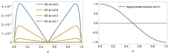
Table 1 displays a comparison between our proposed algorithm at various n for $\mathcal{M}=10$ with the method in [56] in the sense of $L^{\infty }$-error. Figure 1 shows the AE at different values of t (left) and the approximate solution at $t=1$ (right) at $\beta =0.7,n=9$, and $\mathcal{M}=10$. Table 2 and Table 3 report the MAE and the $L^{\infty }$- error at different values of $\mathcal{M}$. In addition, the CPU time (in seconds) for Table 2 is presented in Table 4.

Table 1. Comparison of $L^{\infty }$-error of Example 1.

	Technique in [56]			Our Method at $\mathcal{M}=10$
$\mathit{\beta }$	$\mathit{N}={\mathbf{2}}^{\mathbf{7}}$, $\mathit{M}={\mathbf{2}}^{\mathbf{12}}$	$\mathit{M}={\mathbf{2}}^{\mathbf{7}}$, $\mathit{N}={\mathbf{2}}^{\mathbf{11}}$		$\mathit{n}=\mathbf{2}$	$\mathit{n}=\mathbf{5}$	$\mathit{n}=\mathbf{7}$
0.2	$1.06427\times {10}^{-5}$	$9.66513\times {10}^{-6}$		$5.42251\times {10}^{-7}$	$5.42251\times {10}^{-7}$	$5.42101\times {10}^{-7}$
0.3	$1.06304\times {10}^{-5}$	$9.60898\times {10}^{-6}$		$5.41781\times {10}^{-7}$	$5.41638\times {10}^{-7}$	$5.41301\times {10}^{-7}$
0.4	$1.06126\times {10}^{-5}$	$9.53096\times {10}^{-6}$		$5.30199\times {10}^{-7}$	$5.30219\times {10}^{-7}$	$5.31348\times {10}^{-7}$
0.5	$1.05886\times {10}^{-5}$	$9.42186\times {10}^{-6}$		$5.2937\times {10}^{-8}$	$5.29367\times {10}^{-7}$	$5.29347\times {10}^{-7}$

Figure 1. The AE (left) at different values of t and the approximate solution (right) at $t=1$ of Example 1 at $\beta =0.7,n=9$, and $\mathcal{M}=10$.

Table 2. Errors of Example 1 at $\beta =0.8$ and $n=15$.

$\mathcal{M}$	2	4	6	8	10
MAE	$1.33771\times {10}^{-1}$	$2.28344\times {10}^{-2}$	$1.13447\times {10}^{-3}$	$2.84933\times {10}^{-5}$	$4.25414\times {10}^{-7}$
$L^{\infty }$-error	$2.10514\times {10}^{-1}$	$3.22965\times {10}^{-2}$	$1.44796\times {10}^{-3}$	$3.57062\times {10}^{-5}$	$5.26989\times {10}^{-7}$

Table 3. Errors of Example 1 at $\beta =0.9$ and $n=7$.

$\mathcal{M}$	2	4	6	8	10
MAE	$1.33771\times {10}^{-1}$	$2.27161\times {10}^{-2}$	$1.13171\times {10}^{-3}$	$2.84198\times {10}^{-5}$	$4.24203\times {10}^{-7}$
$L^{\infty }$-error	$2.10514\times {10}^{-1}$	$3.21217\times {10}^{-2}$	$1.44485\times {10}^{-3}$	$3.56291\times {10}^{-5}$	$5.2567\times {10}^{-7}$

Table 4. Our CPU time used for Table 2.

$\mathcal{M}$	2	4	6	8	10
CPU time of MAE	3.157	5.75	13.469	26.827	50.453
CPU time of $L^{\infty }$-error	3.282	5.984	13.672	27.218	50.875

Example 2

([56]). Consider the following fractional Burgers’ equation:

$$\begin{array}{c}\hfill {\displaystyle \frac{{\partial }^{\beta }\chi (\sigma ,t)}{\partial t^{\beta }}}+\chi (\sigma ,t){\displaystyle \frac{\partial \chi (\sigma ,t)}{\partial \sigma }}-{\displaystyle \frac{{\partial }^2\chi (\sigma ,t)}{\partial {\sigma }^2}}={\displaystyle \frac{2}{\mathsf{\Gamma }(3-\beta )}}{e}^{\sigma }{t}^{2-\beta }+t^4{e}^{2\sigma }-t^2{e}^{\sigma },\end{array}$$

(92)

controlled by

$$\begin{array}{cc}& \chi (\sigma ,0)=0,0<\sigma \le 1,\hfill \\ & \chi (0,t)=t^2,\chi (1,t)=e{t}^2,0<t\le 1,\hfill \end{array}$$

(93)

where $\chi (\sigma ,t)=t^2{e}^{\sigma }$ is the exact solution of this problem.

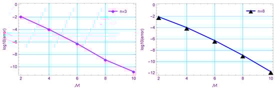
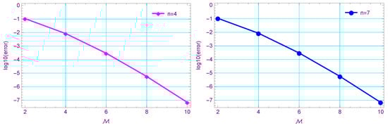
Table 5 reports the AE at $\beta =0.8$ and $\mathcal{M}=10$. In addition, the CPU time (in seconds) for our proposed method is presented in this table. Figure 2 illustrates the Log10(error) at $\beta =0.9$ and different values of n. Table 6 presents a comparison between our method at different values of n at $\mathcal{M}=10$ with the method in [56] in the sense of $L^{\infty }$-error. Also, Table 7 presents a comparison of $L^{\infty }$-error between our method at $n=5$ and $\mathcal{M}=10$ with the method in [68]. Figure 3 shows the AE at different values of t (left) and the approximate solution at $t=1$ (right) at $\beta =0.7,n=10$, and $\mathcal{M}=10$.

Table 5. The AE for Example 2 at $\beta =0.8$ and $\mathcal{M}=10$.

$(\mathit{\sigma },\mathit{t})$	$\mathit{n}=2$	CPU Time	$\mathit{n}=4$	CPU Time	$\mathit{n}=6$	CPU Time
(0.1,0.1)	$1.39127\times {10}^{-13}$		$3.44585\times {10}^{-14}$		$5.65832\times {10}^{-14}$
(0.2,0.2)	$1.26128\times {10}^{-13}$		$1.39194\times {10}^{-14}$		$3.02466\times {10}^{-14}$
(0.3,0.3)	$1.02154\times {10}^{-13}$		$6.84175\times {10}^{-15}$		$5.11952\times {10}^{-14}$
(0.4,0.4)	$4.57134\times {10}^{-14}$		$3.36953\times {10}^{-14}$		$4.39093\times {10}^{-14}$
(0.5,0.5)	$4.28546\times {10}^{-14}$	48.642	$3.61933\times {10}^{-14}$	51.422	$2.95874\times {10}^{-14}$	53.516
(0.6,0.6)	$2.34812\times {10}^{-13}$		$7.54952\times {10}^{-14}$		$2.93099\times {10}^{-13}$
(0.7,0.7)	$8.20677\times {10}^{-13}$		$3.11862\times {10}^{-13}$		$1.22746\times {10}^{-12}$
(0.8,0.8)	$2.49534\times {10}^{-12}$		$8.51985\times {10}^{-13}$		$4.75198\times {10}^{-12}$
(0.9,0.9)	$6.3638\times {10}^{-12}$		$3.50675\times {10}^{-12}$		$1.75979\times {10}^{-11}$

Figure 2. The Log10(error) of Example 2 at $\beta =0.9$ and different values of n.

Table 6. Comparison of $L^{\infty }$-error of Example 2.

	Technique in [56]			Our Method at $\mathcal{M}=10$
$\mathit{\beta }$	$\mathit{N}={\mathbf{2}}^{\mathbf{7}}$, $\mathit{M}={\mathbf{2}}^{\mathbf{11}}$	$\mathit{M}={\mathbf{2}}^{\mathbf{7}}$, $\mathit{N}={\mathbf{2}}^{\mathbf{4}}$		$\mathit{n}=\mathbf{1}$	$\mathit{n}=\mathbf{2}$	$\mathit{n}=\mathbf{3}$
0.2	$5.69465\times {10}^{-7}$	$1.97043\times {10}^{-5}$		$1.17417\times {10}^{-11}$	$1.52283\times {10}^{-11}$	$2.39085\times {10}^{-12}$
0.3	$5.66088\times {10}^{-7}$	$1.99857\times {10}^{-5}$		$2.99682\times {10}^{-12}$	$3.01143\times {10}^{-11}$	$3.59137\times {10}^{-12}$
0.4	$5.61387\times {10}^{-7}$	$2.03716\times {10}^{-5}$		$2.41995\times {10}^{-11}$	$5.67333\times {10}^{-12}$	$2.21096\times {10}^{-12}$
0.5	$5.54967\times {10}^{-7}$	$2.09231\times {10}^{-5}$		$2.12224\times {10}^{-11}$	$1.40504\times {10}^{-11}$	$2.70304\times {10}^{-12}$

Table 7. Comparison of $L^{\infty }$-error of Example 2.

	Technique in [68]
$\mathit{\beta }$	$\mathit{N}={\mathbf{2}}^{\mathbf{7}}$, $\mathit{M}={\mathbf{2}}^{\mathbf{7}}$	$\mathit{N}={\mathbf{2}}^{\mathbf{4}}$	Our Method at $\mathcal{M}=\mathbf{10}$, $\mathit{n}=\mathbf{5}$
0.2	$1.54090\times {10}^{-8}$	$4.2287\times {10}^{-6}$	$7.20079\times {10}^{-12}$
0.3	$1.38810\times {10}^{-8}$	$3.82638\times {10}^{-6}$	$1.00335\times {10}^{-10}$
0.4	$1.18634\times {10}^{-8}$	$3.29441\times {10}^{-6}$	$2.13661\times {10}^{-11}$
0.5	$9.20033\times {10}^{-9}$	$2.58682\times {10}^{-6}$	$2.82427\times {10}^{-11}$

Figure 3. The AE (left) at different values of t and the approximate solution (right) at $t=1$ of Example 2 at $\beta =0.7,n=10$, and $\mathcal{M}=10$.

Remark 8.

Table 8 demonstrates the agreement for both theoretical and numerical results in Figure 2 when $n=3$. As an example, if we set ${\mathcal{K}}_1=0.1,{\mathcal{K}}_2=0.2$, and $n=3$ in Theorem 7.

Table 8. Theoretical error of Example 2.

$\mathcal{M}$	2	4	6	8	10
Error in Theorem 7	$3.733\times {10}^{-1}$	$5.560\times {10}^{-3}$	$4.913\times {10}^{-5}$	$2.854\times {10}^{-7}$	$1.170\times {10}^{-9}$

Remark 9.

The results of Table 6 demonstrate that the approximations corresponding to $n=1$ (the Fermat case) are not always better than the approximations for other choices of n.

Example 3

([56,69]). Consider the following fractional Burgers’ equation:

$$\begin{array}{cc}\hfill {\displaystyle \frac{{\partial }^{\beta }\chi (\sigma ,t)}{\partial t^{\beta }}}+\chi (\sigma ,t){\displaystyle \frac{\partial \chi (\sigma ,t)}{\partial \sigma }}-& 2{\displaystyle \frac{{\partial }^2\chi (\sigma ,t)}{\partial {\sigma }^2}}={\displaystyle \frac{2}{\mathsf{\Gamma }(3-\beta )}}{t}^{2-\beta }sin\left(\pi \sigma \right)\hfill \\ & +\pi t^{4}sin\left(\pi \sigma \right)cos\left(\pi \sigma \right)+2{\pi }^2{t}^{2}sin\left(\pi \sigma \right),\hfill \end{array}$$

(94)

controlled by

$$\begin{array}{cc}& \chi (\sigma ,0)=0,0<\sigma \le 1,\hfill \\ & \chi (0,t)=\chi (1,t)=0,0<t\le 1,\hfill \end{array}$$

(95)

where $\chi (\sigma ,t)=t^{2}sin\left(\pi \sigma \right)$ is the exact solution to (96).

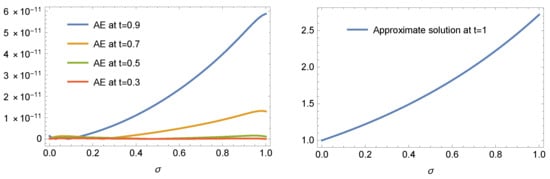
Table 9 displays a comparison between our proposed algorithm at different various n for $\mathcal{M}=10$ with methods in [56,69] in the sense of $L^{\infty }$-error. Also, Table 10 presents a comparison of $L^{\infty }$-error between our method at $n=7$ and $\mathcal{M}=10$ with the method in [68]. Figure 4 shows the AE at different values of t (left) and the approximate solution at $t=1$ (right) at $\beta =0.6,n=5$ and $\mathcal{M}=10$. Table 11 reports the AE at $\beta =0.7$, and $\mathcal{M}=10$. Figure 5 illustrates the Log10(error) at $\beta =0.8$ and different values of n. In addition, the CPU time (in seconds) for our proposed method is presented in this table.

Table 9. Comparison of $L^{\infty }$-error of Example 3.

	Technique in [69]	Technique in [56]		Our Method at $\mathcal{M}=10$
$\mathit{\beta }$	$\mathit{N}={\mathbf{2}}^{\mathbf{7}}$, $\mathit{M}={\mathbf{2}}^{\mathbf{12}}$	$\mathit{N}={\mathbf{2}}^{\mathbf{7}}$, $\mathit{M}={\mathbf{2}}^{\mathbf{12}}$		$\mathit{n}=\mathbf{1}$	$\mathit{n}=\mathbf{2}$	$\mathit{n}=\mathbf{3}$
0.2	$5.47402\times {10}^{-5}$	$4.76511\times {10}^{-5}$		$8.87866\times {10}^{-8}$	$8.89375\times {10}^{-8}$	$8.86872\times {10}^{-8}$
0.3	$5.46367\times {10}^{-5}$	$4.75486\times {10}^{-5}$		$8.87477\times {10}^{-8}$	$8.83007\times {10}^{-8}$	$8.85437\times {10}^{-8}$
0.4	$5.44879\times {10}^{-5}$	$4.74015\times {10}^{-5}$		$8.93898\times {10}^{-8}$	$8.93463\times {10}^{-8}$	$8.79626\times {10}^{-8}$
0.5	$5.42862\times {10}^{-5}$	$4.72029\times {10}^{-5}$		$8.76302\times {10}^{-8}$	$8.78076\times {10}^{-8}$	$8.76954\times {10}^{-8}$

Table 10. Comparison of $L^{\infty }$-error of Example 3.

	Technique in [68]
$\mathit{\beta }$	$\mathit{N}={\mathbf{2}}^{\mathbf{7}}$, $\mathit{M}={\mathbf{2}}^{\mathbf{12}}$	$\mathit{N}={\mathbf{2}}^{\mathbf{9}}$	Our Method at $\mathcal{M}=\mathbf{10}$, $\mathit{n}=\mathbf{7}$
0.2	$5.9687\times {10}^{-6}$	$5.64352\times {10}^{-6}$	$8.88667\times {10}^{-8}$
0.3	$5.95582\times {10}^{-6}$	$5.5615\times {10}^{-6}$	$8.86095\times {10}^{-8}$
0.4	$5.93727\times {10}^{-6}$	$5.4489\times {10}^{-6}$	$8.79734\times {10}^{-8}$
0.5	$5.91227\times {10}^{-6}$	$5.2927\times {10}^{-6}$	$8.76423\times {10}^{-8}$

Figure 4. The AE (left) at different values of t and the approximate solution (right) at $t=1$ of Example 3 at $\beta =0.6,n=5$, and $\mathcal{M}=10$.

Table 11. The AE for Example 3 at $\beta =0.7$ and $\mathcal{M}=10$.

$(\mathit{\sigma },\mathit{t})$	$\mathit{n}=3$	CPU Time	$\mathit{n}=5$	CPU Time	$\mathit{n}=8$	CPU Time
(0.1,0.1)	$6.88724\times {10}^{-10}$		$6.88726\times {10}^{-10}$		$6.88622\times {10}^{-10}$
(0.2,0.2)	$2.5737\times {10}^{-19}$		$2.57334\times {10}^{-9}$		$2.57324\times {10}^{-9}$
(0.3,0.3)	$5.64325\times {10}^{-9}$		$5.643\times {10}^{-9}$		$5.64277\times {10}^{-9}$
(0.4,0.4)	$1.01399\times {10}^{-8}$		$1.01403\times {10}^{-8}$		$1.01399\times {10}^{-8}$
(0.5,0.5)	$1.64631\times {10}^{-8}$	51.627	$1.64642\times {10}^{-8}$	52.204	$1.6464\times {10}^{-8}$	52.063
(0.6,0.6)	$2.51697\times {10}^{-8}$		$2.51707\times {10}^{-8}$		$2.51715\times {10}^{-8}$
(0.7,0.7)	$3.69135\times {10}^{-8}$		$3.69109\times {10}^{-8}$		$3.6915\times {10}^{-8}$
(0.8,0.8)	$5.21996\times {10}^{-8}$		$5.21855\times {10}^{-8}$		$5.21974\times {10}^{-8}$
(0.9,0.9)	$7.01578\times {10}^{-8}$		$7.01168\times {10}^{-8}$		$7.01439\times {10}^{-8}$

Figure 5. The Log10(error) of Example 3 at $\beta =0.8$ and different values of n.

Example 4.

Consider the following fractional Burgers’ equation:

$${\displaystyle \frac{{\partial }^{\beta }\chi (\sigma ,t)}{\partial t^{\beta }}}+\chi (\sigma ,t){\displaystyle \frac{\partial \chi (\sigma ,t)}{\partial \sigma }}-{\displaystyle \frac{{\partial }^2\chi (\sigma ,t)}{\partial {\sigma }^2}}=0,$$

(96)

controlled by

$$\begin{array}{cc}& \chi (\sigma ,0)=0,0<\sigma \le 1,\hfill \\ & \chi (0,t)=t,\chi (1,t)=0,0<t\le 1.\hfill \end{array}$$

(97)

Since the exact solution is not available, let us define the following absolute residual error norm:

$$ARE=\underset{(\sigma ,t)\in (0,1)\times (0,1)}{max}\left|{\displaystyle \frac{{\partial }^{\beta }{\chi }^{\mathcal{M}}(\sigma ,t)}{\partial t^{\beta }}}+{\chi }^{\mathcal{M}}(\sigma ,t){\displaystyle \frac{\partial {\chi }^{\mathcal{M}}(\sigma ,t)}{\partial \sigma }}-{\displaystyle \frac{{\partial }^2{\chi }^{\mathcal{M}}(\sigma ,t)}{\partial {\sigma }^2}}\right|.$$

(98)

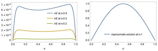
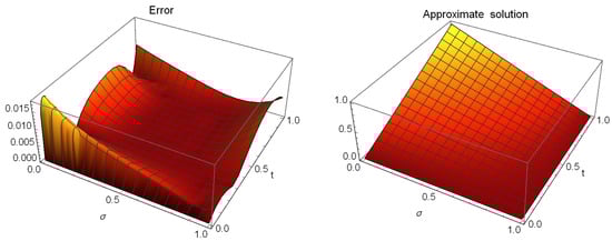
and applying the presented method at $n=1,$$\beta =0.2$, and $\mathcal{M}=10$ to obtain Table 12, which illustrates the ARE at different values of t and the CPU time (in seconds). Figure 6 shows the ARE (left) and the approximate solution (right) at $\beta =0.2,n=1$, and $\mathcal{M}=4$.

Table 12. The ARE for Example 4 at $\beta =0.2$ and $\mathcal{M}=10$.

$\mathit{\sigma }$	$\mathit{t}=3$	$\mathit{t}=6$	$\mathit{t}=8$	CPU Time
0.1	$1.9295\times {10}^{-6}$	$2.31228\times {10}^{-7}$	$2.90447\times {10}^{-6}$
0.2	$1.53756\times {10}^{-6}$	$1.86984\times {10}^{-7}$	$2.204\times {10}^{-6}$
0.3	$1.22152\times {10}^{-6}$	$1.43812\times {10}^{-7}$	$1.66797\times {10}^{-6}$
0.4	$9.61916\times {10}^{-7}$	$1.09957\times {10}^{-7}$	$1.25194\times {10}^{-6}$
0.5	$7.45597\times {10}^{-7}$	$8.29039\times {10}^{-8}$	$9.27122\times {10}^{-7}$	83.014
0.6	$5.61974\times {10}^{-7}$	$6.10056\times {10}^{-8}$	$6.70458\times {10}^{-7}$
0.7	$4.02449\times {10}^{-7}$	$4.29632\times {10}^{-8}$	$4.63476\times {10}^{-7}$
0.8	$2.59984\times {10}^{-7}$	$2.73363\times {10}^{-8}$	$2.9123\times {10}^{-7}$
0.9	$1.25138\times {10}^{-7}$	$2.37574\times {10}^{-8}$	$1.39256\times {10}^{-7}$

Figure 6. The ARE (left) and the approximate solution (right) of Example 4 at $\beta =0.2,n=1$, and $\mathcal{M}=4$.

Remark 10.

The approximate solution at $\beta =0.2,n=1$, and $\mathcal{M}=4$ is

$$\begin{array}{cc}& {\chi }^4(\sigma ,t)=-4.3021142204224816\times {10}^{-15}{\sigma }^4+1.0375381109817283\times {10}^{-14}{\sigma }^3\hfill \\ & -8.784639682346551\times {10}^{-15}{\sigma }^2+3.096915085487595\times {10}^{-15}\sigma \hfill \\ & +\left(-0.0313691{\sigma }^4+0.141414{\sigma }^3-0.262584{\sigma }^2+0.152539\sigma -1.4183099139586375\times {10}^{-14}\right)t^4\hfill \\ & +\left(0.167817{\sigma }^4-0.577364{\sigma }^3+0.822897{\sigma }^2-0.41335\sigma +2.8976820942716586\times {10}^{-14}\right)t^3\hfill \\ & +\left(-0.191013{\sigma }^4+0.806954{\sigma }^3-1.36999{\sigma }^2+0.754052\sigma -1.9734214262712158\times {10}^{-14}\right)t^2\hfill \\ & +\left(0.0460916{\sigma }^4-0.362139{\sigma }^3+0.830823{\sigma }^2-1.51478\sigma +1.\right)t-3.86843335142828\times {10}^{-16}.\hfill \end{array}$$

(99)

7. Concluding Remarks

A numerical algorithm for the fractional Burgers’ equations was presented in this paper. A set of polynomials that generalizes the set of the standard Fermat polynomials was used as basis functions. Some theoretical results regarding these generalized polynomials were developed and used to design our proposed collocation algorithm. Some inequalities were also developed and used to help investigate the convolved Fermat polynomials. The presented numerical algorithm showed the applicability and accuracy of our proposed algorithm. Other convolved polynomials will be a target to investigate in the near future from both theoretical and numerical points of view.

References

- Tarasov, V.E. Fractional Dynamics: Applications of Fractional Calculus to Dynamics of Particles, Fields and Media; Springer: Berlin/Heidelberg, Germany, 2011. [Google Scholar]
- Kilbas, A.A.; Srivastava, H.M.; Trujillo, J.J. Theory and Applications of Fractional Differential Equations; Elsevier: Amsterdam, The Netherlands, 2006; Volume 204. [Google Scholar]
- Atanackovic, T.M.; Pilipovic, S.; Stankovic, B.; Zorica, D. Fractional Calculus with Applications in Mechanics: Wave Propagation, Impact and Variational Principles; John Wiley & Sons: Hoboken, NJ, USA, 2014. [Google Scholar]
- Afreen, A.; Raheem, A. Study of a nonlinear system of fractional differential equations with deviated arguments via Adomian decomposition method. Int. J. Appl. Comput. Math. 2022, 8, 269. [Google Scholar] [CrossRef] [PubMed]
- Obeidat, N.A.; Rawashdeh, M.S.; Al Erjani, M.Q. A novel Adomian natural decomposition method with convergence analysis of nonlinear time-fractional differential equations. Int. J. Model. Simul. 2024. [Google Scholar] [CrossRef]
- Jafari, H.; Jassim, H.K.; Ansari, A.; Nguyen, V.T. Local fractional variational iteration transform method: A tool for solving local fractional partial differential equations. Fractals 2024, 32, 2440022. [Google Scholar] [CrossRef]
- Jose, S.; Parthiban, V. Finite-time synchronization of fractional order neural networks via sampled data control with time delay. J. Math. Comput. Sci. 2024, 35, 374–387. [Google Scholar] [CrossRef]
- Tripura, T.; Chakraborty, S. Wavelet neural operator for solving parametric partial differential equations in computational mechanics problems. Comput. Methods Appl. Mech. Eng. 2023, 404, 115783. [Google Scholar] [CrossRef]
- Zada, L.; Aziz, I. Numerical solution of fractional partial differential equations via Haar wavelet. Numer. Methods Partial Differ. Equ. 2022, 38, 222–242. [Google Scholar] [CrossRef]
- Yuttanan, B.; Razzaghi, M.; Vo, T.N. A numerical method based on fractional-order generalized Taylor wavelets for solving distributed-order fractional partial differential equations. Appl. Numer. Math. 2021, 160, 349–367. [Google Scholar] [CrossRef]
- Kumar, S.; Kumar, R.; Agarwal, R.P.; Samet, B. A study of fractional Lotka-Volterra population model using Haar wavelet and Adams-Bashforth-Moulton methods. Math. Methods Appl. Sci. 2020, 43, 5564–5578. [Google Scholar] [CrossRef]
- Diethelm, K. An efficient parallel algorithm for the numerical solution of fractional differential equations. Frac. Calc. Appl. Anal. 2011, 14, 475–490. [Google Scholar] [CrossRef]
- Farhood, A.K.; Mohammed, O.H. Homotopy perturbation method for solving time-fractional nonlinear variable-order delay partial differential equations. Partial Differ. Equ. Appl. Math. 2023, 7, 100513. [Google Scholar]
- Hafez, R.M.; Youssri, Y.H. Shifted Gegenbauer-Gauss collocation method for solving fractional neutral functional-differential equations with proportional delays. Kragujev. J. Math. 2022, 46, 981–996. [Google Scholar] [CrossRef]
- Hafez, R.M.; Youssri, Y.H. Shifted Jacobi collocation scheme for multidimensional time-fractional order telegraph equation. Iran. J. Numer. Anal. Optim. 2020, 10, 195–223. [Google Scholar]
- Avazzadeh, Z.; Nikan, O.; Nguyen, A.T.; Nguyen, V.T. A localized hybrid kernel meshless technique for solving the fractional Rayleigh–Stokes problem for an edge in a viscoelastic fluid. Eng. Anal. Bound. Elem. 2023, 146, 695–705. [Google Scholar]
- Li, L.; Li, D. Exact solutions and numerical study of time fractional Burgers’ equations. Appl. Math. Lett. 2020, 100, 106011. [Google Scholar]
- Akram, T.; Abbas, M.; Riaz, M.B.; Ismail, A.I.; Ali, N.M. An efficient numerical technique for solving time fractional Burgers equation. Alex. Eng. J. 2020, 59, 2201–2220. [Google Scholar]
- Pirkhedri, A. Applying Haar-Sinc spectral method for solving time-fractional Burger equation. Math. Comput. Sci. 2024, 5, 43–54. [Google Scholar]
- Dwivedi, H.K.; Rajeev. A novel fast second order approach with high-order compact difference scheme and its analysis for the tempered fractional Burgers equation. Math. Comput. Simul. 2025, 227, 168–188. [Google Scholar]
- Singh, J.; Kumar, D.; Swroop, R. Numerical solution of time-and space-fractional coupled Burgers’ equations via homotopy algorithm. Alex. Eng. J. 2016, 55, 1753–1763. [Google Scholar]
- Ali, I.; Haq, S.; Aldosary, S.F.; Nisar, K.S.; Ahmad, F. Numerical solution of one-and two-dimensional time-fractional Burgers equation via Lucas polynomials coupled with Finite difference method. Alex. Eng. J. 2022, 61, 6077–6087. [Google Scholar]
- Mittal, A.K. Spectrally accurate approximate solutions and convergence analysis of fractional Burgers’ equation. Arabian J. Math. 2020, 9, 633–644. [Google Scholar]
- Chawla, R.; Deswal, K.; Kumar, D.; Baleanu, D. Numerical simulation for generalized time-fractional Burgers’ equation with three distinct linearization schemes. J. Comput. Nonlinear Dynam. 2023, 18, 041001. [Google Scholar]
- Huang, Y.; Mohammadi Zadeh, F.; Hadi Noori Skandari, M.; Ahsani Tehrani, H.; Tohidi, E. Space–time Chebyshev spectral collocation method for nonlinear time-fractional Burgers equations based on efficient basis functions. Math. Methods Appl. Sci. 2021, 44, 4117–4136. [Google Scholar] [CrossRef]
- Zongo, G.; Ousséni, S.; Barro, G. a numerical method to solve the viscosity problem of the Burgers equation. Adv. Differ. Equ. Control Process. 2024, 31, 153–164. [Google Scholar] [CrossRef]
- Hamadou, B.; Wassiha, N.A.; Bassono, F.; Youssouf, M.; Moussa, B. approximated solutions of the homogeneous linear fractional diffusion-convection-reaction equation. Adv. Differ. Equ. Control Process. 2024, 31, 257–274. [Google Scholar] [CrossRef]
- Boyd, J.P. Chebyshev and Fourier Spectral Methods; Courier Corporation: Chelmsford, MA, USA, 2001. [Google Scholar]
- Shen, J.; Tang, T.; Wang, L.L. Spectral Methods: Algorithms, Analysis and Applications, 1st ed.; Springer: New York, NY, USA, 2011. [Google Scholar]
- Postavaru, O. An efficient numerical method based on Fibonacci polynomials to solve fractional differential equations. Math. Comput. Simul. 2023, 212, 406–422. [Google Scholar] [CrossRef]
- Manohara, G.; Kumbinarasaiah, S. Numerical solution of a modified epidemiological model of computer viruses by using Fibonacci wavelets. J. Anal. 2024, 32, 529–554. [Google Scholar]
- Singh, P.K.; Ray, S.S. A numerical approach based on Pell polynomial for solving stochastic fractional differential equations. Numer. Algorithms 2024, 97, 1513–1534. [Google Scholar]
- Çerdik Yaslan, H. Pell polynomial solution of the fractional differential equations in the Caputo–Fabrizio sense. Indian J. Pure Appl. Math. 2024. [Google Scholar] [CrossRef]
- Abd-Elhameed, W.M.; Alqubori, O.M.; Atta, A.G. A collocation procedure for treating the time-fractional FitzHugh-Nagumo differential equation using shifted Lucas polynomials. Mathematics 2024, 12, 3672. [Google Scholar] [CrossRef]
- Abd-Elhameed, W.M.; Alqubori, O.M.; Atta, A.G. A collocation approach for the nonlinear fifth-order KdV equations using certain shifted Horadam polynomials. Mathematics 2025, 13, 300. [Google Scholar] [CrossRef]
- Yadav, P.; Jahan, S.; Nisar, K.S. Solving fractional Bagley-Torvik equation by fractional order Fibonacci wavelet arising in fluid mechanics. Ain Shams Eng. J. 2024, 15, 102299. [Google Scholar] [CrossRef]
- Zheng, Z.; Yuan, H.; He, J. A Physics-Informed Neural Network model combined Pell–Lucas polynomials for solving the Lane–Emden type equation. Eur. Phys. J. Plus 2024, 139, 223. [Google Scholar] [CrossRef]
- Chaudhary, R.; Aeri, S.; Bala, A.; Kumar, R.; Baleanu, D. Solving system of fractional differential equations via Vieta-Lucas operational matrix method. Int. J. Appl. Comput. Math. 2024, 10, 14. [Google Scholar]
- Wang, W.; Wang, H. Some results on convolved (p,q)-Fibonacci polynomials. Integral Transform. Spec. Funct. 2015, 26, 340–356. [Google Scholar]
- Ramírez, J.L. On convolved generalized Fibonacci and Lucas Polynomials. Appl. Math. Comput. 2014, 229, 208–213. [Google Scholar]
- Şahin, A.; Ramirez, J.L. Determinantal and permanental representations of convolved Lucas polynomials. Appl. Math. Comput. 2016, 281, 314–322. [Google Scholar]
- Ye, X.; Zhang, Z. A common generalization of convolved generalized Fibonacci and Lucas polynomials and its applications. Appl. Math. Comput. 2017, 306, 31–37. [Google Scholar] [CrossRef]
- Abd-Elhameed, W.M.; Napoli, A. New formulas of convolved Pell polynomials. AIMS Math. 2022, 9, 565–593. [Google Scholar] [CrossRef]
- Abd-Elhameed, W.M.; Alqubori, O.M.; Napoli, A. On convolved Fibonacci polynomials. Mathematics 2024, 13, 22. [Google Scholar] [CrossRef]
- Hafez, R.M.; Youssri, Y.H. Review on Jacobi-Galerkin spectral method for linear PDEs in applied mathematics. Contemp. Math. 2024, 5, 2051–2088. [Google Scholar]
- Zhang, X.; Wang, J.; Wu, Z.; Tang, Z.; Zeng, X. Spectral Galerkin Methods for Riesz Space-Fractional Convection-Diffusion Equations. Fractal Fract. 2024, 8, 431. [Google Scholar] [CrossRef]
- Abd-Elhameed, W.M.; Alsuyuti, M.M. New spectral algorithm for fractional delay pantograph equation using certain orthogonal generalized Chebyshev polynomials. Commun. Nonlinear Sci. Numer. Simul. 2025, 141, 108479. [Google Scholar] [CrossRef]
- Abd-Elhameed, W.M.; Alqubori, O.M.; Al-Harbi, A.K.; Alharbi, M.H.; Atta, A.G. Generalized third-kind Chebyshev tau approach for treating the time fractional cable problem. Elect. Res. Arch. 2024, 32, 6200–6224. [Google Scholar] [CrossRef]
- Masoud, M. Numerical solution of systems of fractional order integro-differential equations with a Tau method based on monic Laguerre polynomials. J. Math. Anal. Model. 2022, 3, 1–13. [Google Scholar] [CrossRef]
- Sadri, K.; Amilo, D.; Hosseini, K.; Hinçal, E.; Seadawy, A.R. A tau-Gegenbauer spectral approach for systems of fractional integrodifferential equations with the error analysis. AIMS Math. 2024, 9, 3850–3880. [Google Scholar] [CrossRef]
- Banihashemi, S.; Jafari, H.; Babaei, A. A stable collocation approach to solve a neutral delay stochastic differential equation of fractional order. J. Comput. Appl. Math. 2022, 403, 113845. [Google Scholar] [CrossRef]
- Wang, F.; Zhao, Q.; Chen, Z.; Fan, C.M. Localized Chebyshev collocation method for solving elliptic partial differential equations in arbitrary 2D domains. Appl. Math. Comput. 2021, 397, 125903. [Google Scholar] [CrossRef]
- Ayalew, M.; Ayalew, M.; Aychluh, M. Numerical approximation of space-fractional diffusion equation using Laguerre spectral collocation method. Int. J. Math. Ind. 2025, 2450029. [Google Scholar] [CrossRef]
- Abd-Elhameed, W.M.; Alqubori, O.M.; Atta, A.G. A collocation procedure for the numerical treatment of the FitzHugh–Nagumo equation using a kind of Chebyshev polynomials. AIMS Math. 2025, 10, 1201–1223. [Google Scholar] [CrossRef]
- Hafez, R.M.; Youssri, Y.H. Legendre-collocation spectral solver for variable-order fractional functional differential equations. Comput. Methods Differ. Equ. 2020, 8, 99–110. [Google Scholar]
- Shafiq, M.; Abbas, M.; Abdullah, F.A.; Majeed, A.; Abdeljawad, T.; Alqudah, M.A. Numerical solutions of time fractional Burgers’ equation involving Atangana–Baleanu derivative via cubic B-spline functions. Results Phys. 2022, 34, 105244. [Google Scholar] [CrossRef]
- Wang, K.L.; He, C.H. A remark on Wang’s fractal variational principle. Fractals 2019, 27, 1950134. [Google Scholar]
- Podlubny, I. Fractional Differential Equations: An Introduction to Fractional Derivatives, Fractional Differential Equations, to Methods of Their Solution and Some of Their Applications; Elsevier: Amsterdam, The Netherlands, 1998; Volume 198. [Google Scholar]
- Raza, N.; Raza, A.; Ullah, M.A.; Gómez-Aguilar, J. Modeling and investigating the spread of COVID-19 dynamics with Atangana-Baleanu fractional derivative: A numerical prospective. Phys. Scr. 2024, 99, 035255. [Google Scholar] [CrossRef]
- Khan, M.A.; Atangana, A. Numerical Methods for Fractal-Fractional Differential Equations and Engineering: Simulations and Modeling; CRC Press: Boca Raton, FL, USA, 2023. [Google Scholar]
- Youssri, Y.H. A new operational matrix of Caputo fractional derivatives of Fermat polynomials: An application for solving the Bagley-Torvik equation. Adv. Differ. Equ. 2017, 2017, 73. [Google Scholar]
- Abd-Elhameed, W.M.; Al-Harbi, M.S.; Atta, A.G. New convolved Fibonacci collocation procedure for the Fitzhugh–Nagumo non-linear equation. Nonlinear Eng. 2024, 13, 20220332. [Google Scholar]
- Koepf, W. Hypergeometric Summation, 2nd ed.; Springer Universitext Series; Springer: Cham, Switzerland, 2014. [Google Scholar]
- Andrews, G.; Askey, R.; Roy, R. Special Functions; Cambridge University Press: Cambridge, UK, 1999; Volume 71. [Google Scholar]
- Luke, Y.L. Inequalities for generalized hypergeometric functions. J. Approx. Theory 1972, 5, 41–65. [Google Scholar]
- Gaunt, R.E. Bounds for modified Struve functions of the first kind and their ratios. J. Math. Anal. Appl. 2018, 468, 547–566. [Google Scholar]
- Jameson, G.J.O. The incomplete gamma functions. Math. Gaz. 2016, 100, 298–306. [Google Scholar]
- Ghafoor, A.; Fiaz, M.; Shah, K.; Abdeljawad, T. Analysis of nonlinear Burgers equation with time fractional Atangana-Baleanu-Caputo derivative. Heliyon 2024, 10, e33842. [Google Scholar] [CrossRef]
- Yadav, S.; Pandey, R.K. Numerical approximation of fractional Burgers equation with Atangana–Baleanu derivative in Caputo sense. Chaos Solitons Fractals 2020, 133, 109630. [Google Scholar]
Disclaimer/Publisher’s Note: The statements, opinions and data contained in all publications are solely those of the individual author(s) and contributor(s) and not of MDPI and/or the editor(s). MDPI and/or the editor(s) disclaim responsibility for any injury to people or property resulting from any ideas, methods, instructions or products referred to in the content. |
© 2025 by the authors. Licensee MDPI, Basel, Switzerland. This article is an open access article distributed under the terms and conditions of the Creative Commons Attribution (CC BY) license (https://creativecommons.org/licenses/by/4.0/).