On Regime Switching Models

Abstract

Regime switching models have been widely studied for their ability to capture the dynamic behavior of time series data and are widely used in economic and financial data analysis. This paper reviews various regime switching models with various regime switching mechanisms, including threshold models, hidden Markov regime switching models, hidden semi-Markov regime switching models, and smooth transition models. The focus is on regime switching models for time series, studying their underlying frameworks, popular variants, and commonly used estimation methods. In addition, six different regime switching models are compared using two real-world datasets.

1. Introduction

Regime switching is a compelling approach for modeling the process of switching between regimes in a time series characterized by different dynamics or characteristics. The two key concepts in regime switching models are the regime itself and the switching mechanism. These regimes arise from structural breaks in the time series, such as financial crises or changes in government policies, and they often represent different market conditions or economic cycles. Examples include bull or bear markets, low- or high-volatility periods, inflation or deflation phases, and growth or recession cycles see e.g., [1]. The regime switching mechanism can be visible or hidden.

Tong [2] first proposed the threshold autoregression (TAR) model in 1978 to capture the dynamics of financial time series data by switching between different regimes. The general form of Tong’s TAR model is given by

$$X_t={\varphi }_0^{\left(S_t\right)}+{\displaystyle \sum _{i=1}^p}{\varphi }_i^{\left(S_t\right)}+{\theta }^{\left(S_t\right)}{a}_t,$$

(1)

where $a_t$ is a sequence of independent and identically distributed (IID) random variables with mean 0 and variance ${\sigma }^2$, and $S_t$ is an indicator variable representing the regimes or states. The value of $S_t$, determined by a threshold variable $s_t$, can be either observable or hidden.

Threshold models are a class of non-linear process designed to provide local linear approximations to underlying non-linear relationships rather than to describe regime switching behavior. To capture regime switching behavior like business cycles, Hamilton [3] extended the regime switching model by introducing a regime switching mechanism based on hidden Markov chains (HMCs) with an unobservable stochastic process $S_t$, called hidden Markov switching (HMS). In this framework, the transitions between regimes are not directly observable; instead, probabilistic inference is used to determine whether and when a regime change is likely to occur based on the time series. In [3,4], an autoregressive conditional heteroskedasticity (ARCH) type models were applied in the regimes.

Ferguson [5] extended the hidden Markov chain (HMC) model to the hidden semi-Markov state transition (HSMS) model, introducing more flexible sojourn distributions $d_k\left(u\right)$ that represent the probability of spending time u in state k. These sojourn distributions $d_k\left(u\right)$ were generalized from the geometric distributions used in HMC to a wider range of discrete and continuous distributions with positive support, such as Poisson, negative binomial, logarithmic, nonparametric, gamma, Weibull, and log-normal distributions [6].

Teräsvirta [7] proposed another regime switching model, the smooth transition autoregressive (STAR) time series model. In this model, regime changes occur gradually rather than abruptly. The smooth transition function $G(s_t;\gamma ,c)$ determines the degree of influence exerted by each regime. $G(s_t;\gamma ,c)$ is continuous and bounded between 0 and 1. The transition variable $s_t$ is usually considered to be a lagged endogenous variable and is defined as $s_t=y_{t-d}$, where $d>0$ is an integer. The parameter $\gamma$ controls the smoothness of the transition, while c represents the threshold between two regimes. A common example of $G(s_t;\gamma ,c)$ is a first-order logistic function:

$$G(s_t;\gamma ,c)=\frac{1}{1+exp\{-\gamma (s_t-c)\}},\gamma >0,$$

(2)

which defines the logistic STAR (LSTAR) model.

This article reviews various regime switching models with different switching mechanisms. Threshold models that depend on observable variables are discussed in Section 2, hidden Markov regime switching models are covered in Section 3, hidden semi-Markov models in Section 4, smooth transition models in Section 5, some new switching mechanisms will be introduced in Section 6. Section 8 concludes this review paper.

2. Threshold Models

Let us start with a simple threshold model example. The autoregressive (AR) model is a popular choice for modeling the time series $y_t$, $t=1,2,\dots ,T$, and its formula is as follows:

$$y_t=\alpha +{\displaystyle \sum _{j=1}^k}{\varphi }_j{y}_{t-j}+{ϵ}_t,$$

where k is the order of the model, $\alpha$ and ${\varphi }_j$, $j=1,2,\dots ,k$, are parameters, and ${ϵ}_t\sim N(0,{\sigma }^2)$ represents white noise.

The regime switching version of the autoregressive model of order k has the following formulation:

$$y_t={\alpha }^{\left(S_t\right)}+{\displaystyle \sum _{j=1}^k}{\varphi }_j^{\left(S_t\right)}{y}_{t-j}+{ϵ}_t,$$

(3)

where ${ϵ}_t\sim N(0,{\left({\sigma }^{\left(S_t\right)}\right)}^2)$. In addition to continuous-valued models such as autoregressive models, discrete-valued models can also be used to model a given regime $S_t$. Many regime switching discrete-valued models have been proposed, such as the models in [8,9,10,11]. The parameters of the model depend on $S_t=i$, where $i=1,2,\dots ,K$, which is an indicator variable representing the regime or state at time t. The parameters vary between K different regimes. The threshold model assumes that $S_t$ is determined by a deterministic function of the observed variable $s_t$. Different types of threshold models may have different deterministic functions of the observed variable $s_t$ or different model specifications within regimes.

Tong and Lim [12] introduced the self-exciting TAR (SETAR) model. In this model, $S_t$ is the lagged endogenous variable $y_{t-d}$. For the SETAR model, $S_t$ is determined as follows:

$$S_t=\left\{\begin{array}{cc}1,\hfill & y_{t-d}<{\tau }_1,\hfill \\ 2,\hfill & {\tau }_1\le y_{t-d},\hfill \\ ⋮\hfill \\ K\hfill & {\tau }_{K-1}\le y_{t-d}.\hfill \end{array}\right.$$

The parameters d and ${\tau }_i$ in the SETAR model represent the “delay” parameter and the thresholds, respectively, both of which are unobservable. $S_t$ determined by d and ${\tau }_i$ is unobservable and needs to be estimated from the data. The threshold variable $S_t$ can also be an exogenous time series $X_t$ [13], a linear combination of lagged or exogenous variables [14,15,16], or a non-linear combination [17,18].

There are different types of threshold models for the financial time series. Chen et al. [19] provided a comprehensive summary of threshold models categorized into three classes: non-linearity in mean, non-linearity in volatility, and ‘double’ threshold dynamics (in both mean and volatility). Non-linearity models in mean include the threshold autoregressive (TAR) model [20,21,22,23,24], the threshold moving-average (TMA) model [25,26], and the threshold autoregressive moving-average (TARMA) model [27,28]. Within each regime, the autoregressive, moving-average (MA), and autoregressive moving-average (ARMA) models are employed.

Non-linearities in volatility models include GJR-GARCH [29], ST-GARCH [30,31], DTGARCH [15], Threshold GJR-GARCH [32], TARR [33], TGARCH [4] and DTGARCH [34]. These models are extensions of one of the most popular volatility models, the GARCH-type model.

To account for non-linearity in the mean and volatility models, Li and Li [35] proposed a DTARCH model to handle asymmetric mean responses in the presence of non-linearities in both mean and volatility. In addition, Brooks [36] extended the DTARCH model to a double threshold GARCH (DT-GARCH) model to assess asymmetries in market indices, stock returns, and exchange rates. Chen and So [15] allowed $S_t$ to be a weighted average of important auxiliary variables, defined as follows:

$$S_t={\displaystyle \sum _{i=1}^l}{w}_i{S}_{it},0\le w_i\le 1,{\displaystyle \sum _{i=1}^l}{w}_i=1.$$

(4)

Here, $S_{it}$ can represent any function of endogenous variables $Y_t,\dots ,Y_1$ and exogenous variables. Therefore, information about both endogenous variables and exogenous variables can be used to govern the switching mechanism. Chen and So [15] found that domestic returns are the main factor determining the threshold compared with international returns. Chen et al. [34,37] proposed a three-regime DTGARCH model to capture the asymmetry in both mean and volatility. Audrino and Bühlmann [38] proposed a tree-based GARCH model. In addition to GARCH-type models, So et al. [39] proposed threshold stochastic volatility (THSV) models. Chen et al. [40] introduced a generalization of the THSV model, incorporating error innovations that follow a standardized t-distribution.

The challenge in estimating threshold models is that the likelihood function is not differentiable with respect to the thresholds and is often multi-modal. Various approaches have been used to estimate the parameters of threshold models. Two-stage methods are commonly used, as described in [12,41]. These methods specify delay parameters and thresholds and then use maximum likelihood estimation (MLE) to estimate the parameters of the model. Researchers are increasingly using Bayesian methods via Markov chain Monte Carlo (MCMC) methods to estimate more complex models, benefiting from improvements in computational speed. Subsequently, all parameters, including the delay parameters and thresholds, can be estimated simultaneously.

3. Hidden Markov Regime Switching Models

Hamilton [3] and Hamilton and Susmel [42] introduced the hidden Markov regime switching model (also called hidden Markov switching model, abbreviated by HMS model) to analyze financial time series and Hamilton and Susmel [42] incorporated the ARCH model within regimes. The regimes are unobservable and are modeled using probabilistic reasoning with a Markov chains, rather than deterministic functions. In contrast to the threshold models, which are used to model non-linearities in data, the Markov regime switching model is used to capture regime switching behaviors, such as business cycles. Since then, hidden Markov regime switching models have been widely used in financial modeling. The HMS model can also be viewed as a type of hidden Markov model (HMM) [43] with continuous observations. HMMs are statistical models designed using a Markov process with hidden states. These models are widely used in speech recognition, bioinformatics, human activity recognition, and other fields.

In the HMS model, $S_t$ represents the latent regime or state at time t. The observations $y_t$, $t=1,\dots ,T$; depend on the emission probabilities $f(y_t\mid S_t=k,{\Theta }_k)$, which depends on the hidden state $S_t$. Here, $f(y_t\mid S_t=k,{\Theta }_k)$ is the conditional distribution of the observations given the hidden state $S_t$, where ${\Theta }_k$ denotes the model parameters under the regime $S_t=k$, $k=1,2,\dots ,K$. The initial probability ${\pi }_k=Pr(S_1=k)$ represents the probability of starting from state k, and the transition probability $p_{ij}$ represents the probability of transitioning from state i to state j.

The two-state HMS model (where $K=2$) remains a popular specification in financial applications. The two states can usually correspond to depreciation and appreciation regimes. The three-state HMS model ($K=3$) is also used in financial applications. The three states can correspond to three different growth rate phases: recession regime, medium growth regime, and high growth regime, as described in [44,45].

In contrast to the threshold model, the hidden state in the Markov regime switching model is unobservable and is modeled by probabilistic reasoning with a Markov chain rather than a deterministic function. The Markov regime switching chain is defined by the transition matrix $\mathit{P}=\left\{p_{ij}\right\}$. For the two-state model, the transition matrix ${\mathit{P}}_{2\times 2}$ is given by

$${\mathit{P}}_{2\times 2}=\left[\begin{array}{cc}{p}_{11}& p_{12}\\ p_{21}& p_{22}\end{array}\right],$$

where

$$p_{ij}=Pr(S_t=j\mid S_{t-1}=i,S_{t-2}=k,\dots ,y_{t-1},y_{t-2},\dots )=Pr(S_t=j\mid S_{t-1}=i).$$

This reflects the Markov property, in contrast to the behavior of the threshold model. In the Markov switching model, regimes evolve exogenously with respect to the time series, whereas the threshold model shows that the regimes evolve endogenously based on the behavior of the observable variables. Markov switching models do not tie regime switching to the behavior of particular observations.

In finance, there are several popular examples of different types of Markov switching models. Hamilton and Susmel [42] and Gray [46] discussed the Markov switching GARCH (MS-GARCH) model to capture the volatility dynamics of financial time series. Krolzig [47] developed the Markov switching vector autoregression (MS-VAR) model using the traditional vector autoregression (VAR) model as the emission distribution. So et al. [48] combined the stochastic volatility model with Markov regime switching to model time-varying volatility. Hardy [49] considered a simplified Markov regime switching model for analyzing complex monthly stock price return data using log-normal distributions within regimes. Shi and Ho [50] first modeled long memory and regime switching via the autoregressive fractional moving average (ARFIMA) and Markov regime switching models. Ma et al. [51] introduced Markov regime switching into the heterogeneous autoregressive model of realized volatility (HAR-RV type) models and evaluated the forecasting performance.

3.1. The Maximum Likelihood Estimation (MLE) Algorithm

Among the estimation methods of the HMS model, likelihood method is one of the main approaches for estimating the model parameters. For example, Hamilton [3] used maximum likelihood estimation (MLE) to estimate the parameters in the HMS model.

Denote by $\Theta$ the vector of all the parameters in an HMS model. For a given $\Theta$, the log-likelihood function is given by

$$L(\Theta )={\displaystyle \sum _{t=1}^T}logf(y_t\mid {\Omega }_t;\Theta ),$$

where $f(·)$ denotes the density function of $y_t$, and ${\Omega }_t=(y_t,y_{t-1},\dots ,y_0)$ represents the observations up to time t.

For the simplest case with $K=2$ regimes, where $S_t=1$ or 2, $Pr(S_t=i\mid {\Omega }_t;\Theta )$ is given as follows:

$$\begin{array}{ll}\hfill Pr(S_t=i\mid {\Omega }_t;\Theta )& ={\displaystyle \sum _{j=1}^2}Pr(S_t=i\mid S_{t-1}=j,{\Omega }_{t-1};\Theta )Pr(S_{t-1}=j\mid {\Omega }_{t-1};\Theta )\hfill \\ \hfill & ={\displaystyle \sum _{j=1}^2}{p}_{ji}Pr(S_{t-1}=j\mid {\Omega }_{t-1};\Theta ),\hfill \end{array}$$

(5)

where $p_{ji}$ denotes the transition probabilities between regimes. The likelihood of the observations, $f(y_t\mid {\Omega }_t;\Theta )$, is then computed as follows:

$$\begin{array}{ll}\hfill f(y_t\mid {\Omega }_t;\Theta )& ={\displaystyle \sum _{i=1}^2}f(y_t\mid S_t=i,{\Omega }_t;\Theta )Pr(S_t=i\mid {\Omega }_t;\Theta )\hfill \\ \hfill & ={\displaystyle \sum _{i=1}^2}f(y_t\mid S_t=i,{\Omega }_t;\Theta ){\displaystyle \sum _{j=1}^2}{p}_{ji}Pr(S_{t-1}=j\mid {\Omega }_{t-1};\Theta )\hfill \\ \hfill & =f(y_t\mid S_t=1,{\Omega }_t;\Theta )p_{11}Pr(S_{t-1}=1\mid {\Omega }_{t-1};\Theta )\hfill \\ \hfill & +f(y_t\mid S_t=1,{\Omega }_t;\Theta )p_{21}Pr(S_{t-1}=2\mid {\Omega }_{t-1};\Theta )\hfill \\ \hfill & +f(y_t\mid S_t=2,{\Omega }_t;\Theta )p_{12}Pr(S_{t-1}=1\mid {\Omega }_{t-1};\Theta )\hfill \\ \hfill & +f(y_t\mid S_t=2,{\Omega }_t;\Theta )p_{22}Pr(S_{t-1}=2\mid {\Omega }_{t-1};\Theta ).\hfill \end{array}$$

(6)

If we use the regime switching AR(1) model (Equation (3) with $k=1$) as the state-dependent model, the conditional likelihood function in Equation (6) is expressed as follows:

$$\begin{array}{ll}\hfill f(y_t\mid S_t=i,{\Omega }_t;\Theta )& =\frac{1}{{\sigma }_i\sqrt{2\pi }}exp\left\{-\frac{{(y_t-{\alpha }_i-{\varphi }_{1,i}{y}_{t-1})}^2}{2{\sigma }_i^2}\right\},\hfill \end{array}$$

(7)

where $\Theta =({\alpha }_1,{\alpha }_2,{\varphi }_{1,1},{\varphi }_{1,2},{\sigma }_1,{\sigma }_2)$. By Bayes’ rule, the posterior probability of regime i at time t is

$$\begin{array}{l}\hfill Pr(S_t=i\mid {\Omega }_t;\Theta )=\frac{f(y_t\mid S_t=i,{\Omega }_{t-1};\Theta )Pr(S_t=i\mid {\Omega }_{t-1})}{f(y_t\mid {\Omega }_{t-1};\Theta )}.\end{array}$$

(8)

The right-hand side of (8) is obtained using Equations (5) and (7).

To initialize the model, we calculate the initial probabilities as follows:

$$\begin{array}{ll}\hfill Pr(S_1=1\mid y_1,\Theta )& =\frac{f(S_1=1,y_1\mid \Theta )}{f(y_1\mid {\Omega }_0,\Theta )}\hfill \\ \hfill & =\frac{f(S_1=1,y_1\mid \Theta )}{{\sum }_{i=1}^{2}f(S_1=i,y_1\mid \Theta )}\hfill \\ \hfill & =\frac{{\pi }_{1}f(y_1\mid S_1=1,{\Omega }_0;\Theta )}{{\sum }_{i=1}^2{\pi }_{i}f(y_1\mid S_1=i,{\Omega }_0;\Theta )},\hfill \end{array}$$

where ${\pi }_1$ and ${\pi }_2$ are the initial probabilities. These probabilities can be derived by solving the following stationary condition:

$$\begin{array}{ll}\hfill \mathit{\pi }\mathit{P}& =\mathit{\pi },\hfill \\ \hfill \left[\begin{array}{cc}{\pi }_1& {\pi }_2\end{array}\right]\left[\begin{array}{cc}{p}_{11}& p_{12}\\ p_{21}& p_{22}\end{array}\right]& =\left[\begin{array}{cc}{\pi }_1& {\pi }_2\end{array}\right].\hfill \end{array}$$

(9)

It is noted that $\mathit{P}$ above cannot be the identity matrix. Otherwise, regime switching would not occur, and they will depend solely on the initial probabilities, even in the presence of stationary distributions. Solving Equation (9) yields

$$\begin{array}{l}\hfill {\pi }_1=\frac{p_{21}}{p_{12}+p_{21}},{\pi }_2=1-{\pi }_1=\frac{p_{12}}{p_{12}+p_{21}}.\end{array}$$

(10)

Using these initial probabilities, we can recursively update $Pr(S_t=i\mid {\Omega }_t;\Theta )$ via Equation (8) if $Pr(S_{t-1}=i\mid {\Omega }_{t-1};\Theta )$, which follows an AR(1) model (Equation (3) with $k=1$) model here, is known. Finally, the likelihood function $L(\Theta )$ can be constructed recursively, allowing the parameters to be estimated by maximizing the likelihood function.

3.2. The Expectation-Maximization (EM) Algorithm

In some cases, directly maximizing the likelihood of the observed data can be challenging. For example, Augustyniak [52] applied the EM algorithm and an importance sampling method to improve the performance of MLE in the Markov-switching GARCH model. The EM algorithm provides an alternative technique to obtain the MLE of the likelihood of the observed data through an iterative process without directly calculating the likelihood function.

The EM algorithm consists of two steps, the E-step and the M-step, as described below:

• E-step: Compute the expected complete data log-likelihood to obtain the Q-function, $Q(\mathbf{\Phi }\mid {\mathbf{\Phi }}^{(\ell )})$, based on the observed data ${\Omega }_T$ and the current estimate of the parameters, ${\mathbf{\Phi }}^{(\ell )}$, at the ℓ-th iteration:

  $$\begin{array}{ll}\hfill Q(\mathbf{\Phi }\mid {\mathbf{\Phi }}^{(\ell )})& =E_{{\mathbf{\Phi }}^{(\ell )}}\left[logL(\mathbf{\Phi })\mid {\Omega }_T\right]\hfill \\ \hfill & ={\displaystyle \sum _{j=1}^K}{\displaystyle \sum _{t=1}^T}logf(y_t\mid S_t=j,{\Omega }_t;{\mathbf{\Phi }}^{(\ell )})Pr(S_t=j\mid {\Omega }_t;{\mathbf{\Phi }}^{(\ell )}).\hfill \end{array}$$
  If we use the regime switching AR(1) model (Equation (3) with k = 1) as the state-dependent model, $f(y_t\mid S_t=j,{\Omega }_t;{\mathbf{\Phi }}^{(\ell )})$ is the same as in Equation (7), and $Pr(S_t=j\mid {\Omega }_t;{\mathbf{\Phi }}^{(\ell )})$ is the same as in Equation (8).
• M-step: Maximize the Q-function with respect to $\mathbf{\Phi }$, i.e.,

  $$\widehat{\mathbf{\Phi }}=arg\underset{\mathbf{\Phi }}{max}Q(\mathbf{\Phi }\mid {\mathbf{\Phi }}^{(\ell )}).$$

Here, $\mathbf{\Phi }=\{\Theta ,\mathit{\pi },\mathit{P}\}$ denotes the set of model parameters. The above two steps are iterated until convergence, at which point the parameter estimates $\widehat{\mathbf{\Phi }}$ stabilize.

3.3. The Markov Chain Monte Carlo (MCMC) Algorithm

The Markov chain Monte Carlo (MCMC) algorithm is a commonly used approach for HMS estimation. For instance, Amisano and Fagan [53] estimated parameters via the MCMC algorithm because their model exhibited a highly irregular likelihood surface, which makes it challenging to estimate parameters via maximum likelihood estimation. A joint posterior distribution for the parameters and latent variables is obtained by the Bayesian approach. This is done through Gibbs sampling-based posterior simulation. Kim and Nelson [54] described in detail in Chapter 9 how to use the Gibbs sampling method in the HMS model. Within the HMS framework, the model’s unknown parameters $\Theta$ are estimated first. Then, the latent regime $S_t$ conditional on parameters $\Theta$ is estimated. In the Bayesian analysis, both parameters $\Theta$ and latent regime $S_t$ are treated as random variables. The key to the Bayesian approach is that the unknown parameters $\Theta$ are treated as random variables. The joint posterior density is derived as follows:

$$\begin{array}{ll}\hfill f({\tilde{S}}_T,\Theta ,\mathcal{P},\mid {\Omega }_T)& =f(\Theta ,\mathcal{P}\mid {\Omega }_T,{\tilde{S}}_T)Pr({\tilde{S}}_T,\mid {\Omega }_T)\hfill \\ \hfill & =f(\Theta \mid {\Omega }_T,{\tilde{S}}_T)f(\mathcal{P}\mid {\Omega }_T,{\tilde{S}}_T)Pr({\tilde{S}}_T,\mid {\Omega }_T)\hfill \\ \hfill & =f(\Theta \mid {\Omega }_T,{\tilde{S}}_T)f(\mathcal{P}\mid {\tilde{S}}_T)Pr({\tilde{S}}_T,\mid {\Omega }_T),\hfill \end{array}$$

(11)

where ${\tilde{S}}_T={(S_1,S_2,\dots ,S_T)}^{\top },\mathcal{P}=\{p_{11},p_{22}\}$. Equation (11) assumes that the transition probabilities in $\mathcal{P}$ given ${\tilde{S}}_T$ are independent of other parameters $\Theta$ and the observed data ${\Omega }_T$ so that $f(\mathcal{P}\mid {\Omega }_T,{\tilde{S}}_T)=f(\mathcal{P}\mid {\tilde{S}}_T)$. We then apply the Gibbs sampling as follows:

• Generate $S_t$ from $f(S_t\mid {\tilde{S}}_{\ne t},\Theta ,\mathcal{P},{\Omega }_T),t=1,2,\dots ,T$, where
  ${\tilde{S}}_{\ne t}={(S_1,\dots ,S_{t-1},S_{t+1},\dots ,S_T)}^{\top }$ is a vector of S variables that exclude $S_t$;
  or generate ${\tilde{S}}_T$ from $f({\tilde{S}}_T\mid \Theta ,p_{11},p_{22},{\Omega }_T),t=1,2,\dots ,T$.
• Generate transition probabilities $\mathcal{P}=\{p_{11},p_{22}\}$ from $f(\mathcal{P}\mid {\tilde{S}}_T)$.
• Generate $\Theta =({\mu }_1,{\mu }_2,{\sigma }_1,{\sigma }_2)$ from $f(\Theta \mid {\Omega }_T,{\tilde{S}}_T)$.

These three steps are iterated until convergence. The detailed implementation is given below.

3.3.1. Step 1

There are two generation methods. The first is single-step Gibbs sampling, which generates $S_t$ based on $f(S_t\mid {\tilde{S}}_{\ne t},\Theta ,\mathcal{P},{\Omega }_T)$, $t=1,2,\dots ,T$. By suppressing the conditioning on the parameters, $S_t$ is generated by $f(S_t\mid {\tilde{S}}_{\ne t},{\Omega }_T)$, and the following results can be derived:

$$\begin{array}{l}\hfill f(S_t\mid {\tilde{S}}_{\ne t},{\Omega }_T)\propto f(S_t\mid S_{t-1})f(y_t\mid S_t)f(S_{t+1}\mid S_t).\end{array}$$

(12)

For the derivation process, see Section 9.1.1 of [54]. Using Equation (12), $Pr(S_t=j\mid {\tilde{S}}_{\ne t},{\Omega }_T)$ can be calculated as

$$\begin{array}{l}\hfill Pr(S_t=j\mid {\tilde{S}}_{\ne t},{\Omega }_T)=\frac{f(S_t=j\mid {\tilde{S}}_{\ne t},{\Omega }_T)}{{\sum }_{j=1}^{2}f(S_t=j\mid {\tilde{S}}_{\ne t},{\Omega }_T)}.\end{array}$$

Then, $S_t$ can be generated using a uniform distribution. If the random number generated from $U(0,1)$ is less than $Pr(S_t=j\mid {\tilde{S}}_{\ne t},{\Omega }_T)$, then $S_t=1$; otherwise, $S_t=2$.

Similarly, the second method is multi-move Gibbs sampling, which generates $S_t$ based on $f({\tilde{S}}_T\mid \Theta ,\mathcal{P},{\Omega }_T)$, $t=1,2,\dots ,T$. Finally, $Pr(S_t=j\mid {\tilde{S}}_{t+1},{\Omega }_T)$ can be calculated by the following formula:

$$\begin{array}{l}\hfill Pr(S_t=j\mid S_{t+1},{\Omega }_T)=\frac{f(S_{t+1}\mid S_t=j)f(S_t=j\mid {\Omega }_T)}{{\sum }_{j=1}^{2}f(S_{t+1}\mid S_t=j)f(S_t=j\mid {\Omega }_T)}.\end{array}$$

The derivation is given in Section 9.1.1 of [54]. Then, $S_t$ can be generated by a random variable drawn from $U(0,1)$ based on $Pr(S_t=j\mid S_{t+1},{\Omega }_T)$, which is similar to the single-step Gibbs sampling method.

3.3.2. Step 2

Kim and Nelson [54] used the beta distribution as a conjugate prior for the transition probabilities. The proposed posterior distribution is given by the following two independent beta distributions:

$$\begin{array}{l}\hfill p_{11}\mid {\tilde{S}}_T\sim \mathrm{Beta}(u_{11}+n_{11},u_{12}+n_{12}),\\ \hfill p_{22}\mid {\tilde{S}}_T\sim \mathrm{Beta}(u_{22}+n_{22},u_{21}+n_{21}),\end{array}$$

where $u_{ij}$ is a known prior hyper-parameter and $n_{ij}$ represents the transitions from state i to j, which can be easily calculated for a given ${\tilde{S}}_T$.

3.3.3. Step 3

The last step is based on the parameters in the state-dependent model, which need to be derived from different models. An example in [54] is about generating ${\mu }_1$ and ${\mu }_2$, conditional on ${\sigma }_1^2,{\sigma }_2^2,{\Omega }_T,{\tilde{S}}_T$. They assumed a normal prior for $\mu$ as follows:

$$\tilde{\mu }\mid {\sigma }_1^2,{\sigma }_2^2\sim N(b_0,B_0),$$

where $\tilde{\mu }={({\mu }_1,{\mu }_2)}^{\top }$. The posterior distribution is given by

$$\tilde{\mu }\mid {\sigma }_1^2,{\sigma }_2^2,{\Omega }_T,{\tilde{S}}_T\sim N(b_1,B_1),$$

where $b_1={(B_0^{-1}+X^{\top }X)}^{-1}(B_0^{-1}{b}_0+X^{\top }(X\tilde{\mu }+V))$ and $B_1={(B_0^{-1}+X^{\top }X)}^{-1}$, $X=(\frac{1}{{\sigma }_{S_t}},\frac{S_t}{{\sigma }_{S_t}})$, and $V\sim N(0,I_T)$. The parameters ${\mu }_1$ and ${\mu }_2$ can be generated based on the posterior distribution.

3.4. Other Algorithms

In addition, Francq and Zakoı [55] employed the generalized method of moments (GMM) to estimate the MS-GARCH parameters. GMM provides an alternative to simulation-based methods such as MCMC, which typically require more computational power. For moderately large samples, GMM performs well.

Furthermore, Zheng et al. [56] proposed a spectral clustering hidden Markov model that extracts information using spectral methods. Spectral methods aim to reveal the relationship between hidden states and observations through singular value decomposition (SVD) to relate past and future observations. Zheng et al. [56] extended the spectral method of discrete HMMs with discrete observations to accommodate continuous observations, which can be used for HMS models. The advantages of spectral methods include scalability, strong theoretical properties, and the fact that no likelihood function is required.

4. Hidden Semi-Markov State Transition Models

HMS has been extended and adapted into more complex models, such as hidden semi-Markov models (HSMMs), for tasks where HMS faces limitations. Note that the HMS model has two strong assumptions. First, the current latent state depends only on the most recent state in the past, i.e., $Pr(S_t\mid S_{t-1},\dots ,S_1)=Pr(S_t\mid S_{t-1})$. Second, the time spent in a state follows a geometric distribution. Let $d_k\left(u\right)$ be the probability that time u is spent in state k, called the sojourn distribution or duration distribution. In the HMS model, $d_k\left(u\right)$ is simply shown to be geometrically distributed [57].

In fact, the two strong assumptions mentioned above limit the scope and flexibility of possible applications of the HMS model. If the underlying process does not follow a geometric sojourn distribution, the HMS model may not be appropriate. More drawbacks of the HMS model can be found in [58,59]. To overcome the inflexibility, Ferguson Ferguson [5] proposed a hidden semi-Markov state switching (HSMS) model that allows for arbitrary sojourn distributions with great flexibility, including discrete and continuous distributions with positive support, such as Poisson, negative binomial, logarithmic, nonparametric, gamma, Weibull, log-normal [6].

In the hidden semi-Markov switching model, we still use the following notations as in HMS models:

• the initial probabilities ${\pi }_k=Pr(S_1=k)$;
• the emission probabilities $f(y_t\mid S_t=k,{\Theta }_k)$;
• the transition matrix $\mathit{P}=\left\{p_{ij}\right\}$, where $p_{ij}=Pr[S_t=j|S_{t-1}=i]$.

In addition, the probability $d_k\left(u\right)$ of the hidden process $\left\{S_t\right\}$ staying in the kth state for a time u, is defined in HSMS model as follows:

$$d_k\left(u\right)=Pr(S_{t+u}\ne k,S_{t+u-1}=k,\dots ,S_{t+1}=k\mid S_t=k,S_{t-1}\ne k).$$

Ferguson [5] pointed out that speech recognition is one of the earliest and most successful implementations of HSMS. Over time, this approach has been extended to different domains, including the recognition of printed text, handwriting, human DNA sequences, film events, symbolic plan, and language. Its versatility has also inspired many other applications, such as ground target tracking, mobility tracking in cellular networks, protein structure prediction, air particle prediction, speech synthesis, music classification, image segmentation, electrocardiogram segmentation, and financial time series modeling. Yu [60] gave an overview of these applications, while Balcilar et al. [61] used the HSMS model to study various stages of human information processing. Based on the HSMS framework, Xiao and Dong [62] introduced an innovative reputation management system for the online-to-offline (O2O) e-commerce market. There are also some applications of the HSMS model in the financial field. Bernardi et al. [63] constructed an HSMS model with Student-t distribution for tail risk interdependence. Maruotti et al. [59] introduced an HSMS model with a multivariate leptokurtic-normal distribution. Maruotti et al. [57] combined the HSMS model with quantile regression for time series. Qin et al. [64] proposed a robust HSMS model with Huber’s least favorable distribution.

The expectation-maximization (EM) algorithm and forward-backward algorithm are commonly used to estimate parameters $\mathbf{\Phi }=\{\Theta ,\mathit{\pi },\mathit{P},\mathit{D}\}$ in the HSMS models, where $\mathit{D}=\{d_k\left(u\right):u=1,\dots ,U,k=1,\dots ,K-1\}$. If we continue with the AR(1) model (Equation (3) with $k=1$) as a simple state-dependent example, the parameter set is given by $\Theta =({\alpha }_1,{\alpha }_2,{\varphi }_{1,1},{\varphi }_{1,2},{\sigma }_1,{\sigma }_2)$. Through simple calculation, the Q function in the HSMS model becomes the following formula:

$$\begin{array}{l}\hfill Q(\mathbf{\Phi }\mid {\mathbf{\Phi }}^{(\ell )})=Q_1\left(\mathit{\pi }\right)+Q_2\left(\mathit{P}\right)+Q_3\left(\mathit{D}\right)+Q_4(\Theta ),\end{array}$$

(13)

where

$$\begin{array}{ll}\hfill Q_1\left(\mathit{\pi }\right)& ={\displaystyle \sum _{k=1}^K}log{\pi }_{k}Pr(S_1=k\mid {\Omega }_T;{\mathbf{\Phi }}^{(\ell )}),\hfill \\ \hfill Q_2\left(\mathit{P}\right)& ={\displaystyle \sum _{t=1}^{T-1}}{\displaystyle \sum _{k=1}^K}{\displaystyle \sum _{j\ne k}}log{p}_{jk}Pr(S_{t+1}=k,S_t=j\mid {\Omega }_T;{\mathbf{\Phi }}^{(\ell )}),\hfill \\ \hfill Q_3\left(\mathit{D}\right)& ={\displaystyle \sum _{t=1}^T}{\displaystyle \sum _{k=1}^K}{\displaystyle \sum _u}log{d}_k\left(u\right)Pr(S_{t+u+1}=k,\dots ,S_t=k\mid {\Omega }_T;{\mathbf{\Phi }}^{(\ell )}),\hfill \\ \hfill Q_4(\Theta )& ={\displaystyle \sum _{t=1}^T}{\displaystyle \sum _{k=1}^K}logf(y_t\mid S_t=k)Pr(S_t=k\mid {\Omega }_T;{\mathbf{\Phi }}^{(\ell )}).\hfill \end{array}$$

5. Smooth Transition Models

Teräsvirta [7] and Eitrheim and Teräsvirta [65] first introduced and discussed the smooth transition (ST) model and related procedures. The autoregressive model that allows for regime switching in Equation (3) can also be viewed as

$$\begin{array}{l}\hfill y_t={\varphi }_0\left(S_t\right)+{\displaystyle \sum _{i=1}^p}{\varphi }_i\left(S_t\right)y_{t_i}+{\epsilon }_t,t=1,\dots ,T,\end{array}$$

(14)

where ${\varphi }_0\left(S_t\right),{\varphi }_1\left(S_t\right),\dots ,{\varphi }_p\left(S_t\right)$ is a function of the state $S_t$. The regime $S_t$ can be represented by the vector ${\mathit{x}}_t={(1,y_{t-1},\dots ,y_{t-p},s_{1t},\dots ,s_{kt})}^{\top }$, where $s_{1t},\dots ,s_{kt}$ are observable variables. Then, Equation (14) can be written as

$$\begin{array}{l}\hfill y_t={\varphi }_0\left({\mathit{x}}_t\right)+{\displaystyle \sum _{i=1}^p}{\varphi }_i\left({\mathit{x}}_t\right)y_{t_i}+{\epsilon }_t,t=1,\dots ,T,\end{array}$$

(15)

where ${\varphi }_j\left({\mathit{x}}_t\right),j=0,\dots ,p$ can be estimated by nonparametric estimation methods.

For the observed data $y_t$, where $t=1,2,\dots ,T$, the smooth transition model is as follows:

$$\begin{array}{l}\hfill y_t={\mathit{\varphi }}_1^{\top }\left({\mathit{x}}_t\right)(1-G(s_t;\gamma ,c))+{\mathit{\varphi }}_2^{\top }\left({\mathit{x}}_t\right)G(s_t;\gamma ,c)+{\epsilon }_t,t=1,\dots ,T,\end{array}$$

(16)

where ${\mathit{x}}_t={(1,y_{t-1},\dots ,y_{t-p},s_{1t},\dots ,s_{kt})}^{\top }$ consists of lagged endogenous and exogenous variables. The coefficients are denoted as ${\mathit{\varphi }}_i={({\varphi }_{i,0},{\varphi }_{i,1},\dots ,{\varphi }_{i,m})}^{\top }$, where $i=1,2$ and $m=p+k$. The variables $s_{1t},\dots ,s_{kt}$ are observable and exogenous. The transition function $G(s_t;\gamma ,c)$ is continuous and bounded between 0 and 1. The transition variable $s_t$ can be a lagged endogenous variable ($s_t=y_{t-d}$ for a certain integer $d>0$), an exogenous variable ($s_t=z_t$, where $z_t$ is exogenous), or a function of lagged endogenous and exogenous variables. A popular choice for $s_t$ is the lagged endogenous variable $y_{t-d}$. The threshold between the two regimes is denoted by c, and the smoothness of the transition is controlled by the parameter $\gamma$.

We consider the AR(1) model (Equation (3) with $k=1$) as a simple state-dependent example with the number of states being $K=2$. The smooth transition autoregressive (STAR) model is given as follows:

$$\begin{array}{l}\hfill y_t=({\alpha }_1+{\varphi }_{1,1}{y}_{t-1})(1-G(s_t;\gamma ,c))+({\alpha }_2+{\varphi }_{1,2}{y}_{t-1})G(s_t;\gamma ,c)+{ϵ}_t.\end{array}$$

The STAR model is a regime switching model with two regimes, corresponding to $G(s_t;\gamma ,c)=0$ and $G(s_t;\gamma ,c)=1$. Moreover, the transition between the two regimes is gradual because it depends on the smooth variation of the transition function $G(s_t;\gamma ,c)$. As an example, we use the logistic STAR (LSTAR) model, where the transition function $G(s_t;\gamma ,c)$ is defined in Equation (2) and discussed in Section 1. We further consider $s_t=y_{t-d}$, which leads to the self-excited TAR model as described in Section 2. When $\gamma \to 0$, the value of the transition function $G(s_t;\gamma ,c)$ approaches 0.5. Therefore, when $\gamma =0$, the LSTAR model degenerates into a linear model.

In the LSTAR model, the two regimes are usually associated with smaller and larger values of $s_t$ associated with a threshold c. This type of transition function is particularly suitable for modeling business cycles. The LSTAR model with $s_t=y_{t-d}$ can describe periods of positive and negative growth. However, there are other types of regime switching behavior. If regime transitions are associated with smaller and larger absolute values of $s_t$, then the exponential STAR (ESTAR) model with the following $G(s_t;\gamma ,c)$ is more appropriate:

$$\begin{array}{l}\hfill G(s_t;\gamma ,c)=1-exp\{-\gamma {(s_t-c)}^2\},\gamma >0.\end{array}$$

For example, Michael et al. [66] and Baum et al. [67] applied the ESTAR model to real exchange rates. The ESTAR model becomes linear for both $\gamma \to 0$ and $\gamma \to \infty$. Unlike the LSTAR model, the ESTAR model does not nest SETAR as a special case.

In order to overcome the limitations of SETAR, Jansen and Teräsvirta [68] proposed a quadratic logistic function

$$G(s_t;\gamma ,c)=\frac{1}{1+exp\{-\gamma (s_t-c_1)(s_t-c_2)\}},c_1\le c_2,\gamma >0.$$

This STAR model can nest a three-state SETAR model as a special case.

The smooth transition model mentioned above is a basic smooth transition model that only allows the transition function $G(s_t;\gamma ,c)$ to handle two regimes. To overcome this limitation, the model has also been extended to incorporate multiple regimes, accounting for three business cycle phases: depreciation period, slow appreciation, and strong appreciation.

The Equation (16) can be rewritten as

$$\begin{array}{l}\hfill y_t={\mathit{\varphi }}_1^{\top }\left(x_t\right)+{({\mathit{\varphi }}_2\left(x_t\right)-{\mathit{\varphi }}_1\left(x_t\right))}^{\top }G(s_t;\gamma ,c)+{\epsilon }_t.\end{array}$$

(17)

This can then be extended to a three-regime model by adding a second non-linear component as follows:

$$\begin{array}{l}\hfill y_t={\mathit{\varphi }}_1^{\top }\left(x_t\right)+{({\mathit{\varphi }}_2\left(x_t\right)-{\mathit{\varphi }}_1\left(x_t\right))}^{\top }{G}_1(s_t;{\gamma }_1,c_1)+{({\mathit{\varphi }}_3\left(x_t\right)-{\mathit{\varphi }}_2\left(x_t\right))}^{\top }{G}_2(s_t;{\gamma }_2,c_2)+{\epsilon }_t.\end{array}$$

(18)

Assuming that $c_1<c_2$, the autoregressive parameters in this model change smoothly from ${\varphi }_1$ to ${\varphi }_3$ as $s_t$ increases.

More generally, it can be extended to an m-regime model with $m-1$ smoothing parameters ${\gamma }_1,\dots ,{\gamma }_{m-1}$ and thresholds $c_1,\dots ,c_{m-1}$, as shown below:

$$\begin{array}{l}\hfill y_t={\mathit{\varphi }}_1^{\top }\left(x_t\right)+{\displaystyle \sum _{i=1}^{m-1}}{({\mathit{\varphi }}_{i+1}\left(x_t\right)-{\mathit{\varphi }}_i\left(x_t\right))}^{\top }{G}_i(s_t;{\gamma }_i,c_i)+{\epsilon }_t.\end{array}$$

Another way to extend the basic model to a four-regime model is to nest two different two-regime smooth transition models, as shown in the following equation:

$$\begin{array}{l}\hfill \begin{array}{ll}\hfill y_t& =[{\mathit{\varphi }}_1^{\top }\left(x_t\right)(1-G_1(s_{1t};{\gamma }_1,c_1))+{\mathit{\varphi }}_2^{\top }\left(x_t\right)G_1(s_{1t};{\gamma }_1,c_1)](1-G_2(s_{2t};{\gamma }_2,c_2))+\hfill \\ \hfill & +[{\mathit{\varphi }}_3^{\top }\left(x_t\right)(1-G_1(s_{1t};{\gamma }_1,c_1))+{\mathit{\varphi }}_4^{\top }\left(x_t\right)G_1(s_{1t};{\gamma }_1,c_1)]G_2(s_{2t};{\gamma }_2,c_2)+{\epsilon }_t.\hfill \end{array}\end{array}$$

(19)

A further extension of the multi-regime model discussed in the previous paragraphs is the time-varying smooth transition autoregressive (TV-STAR) model, which allows for both non-linear dynamics and time-varying parameters. The TV-STAR model is derived from Equation (19) by setting $s_{1t}=y_{t-d}$ and $s_{2t}=y_t$, using a simplified notation for the transition functions, as shown below:

$$\begin{array}{l}\hfill \begin{array}{ll}\hfill y_t& =[{\mathit{\varphi }}_1^{\top }\left(x_t\right)(1-G_1\left(y_{t-d}\right))+{\mathit{\varphi }}_2^{\top }\left(x_t\right)G_1\left(y_{t-d}\right)](1-G_2\left(y_t\right))+\hfill \\ \hfill & +[{\mathit{\varphi }}_3^{\top }\left(x_t\right)(1-G_1\left(y_{t-d}\right))+{\mathit{\varphi }}_4^{\top }\left(x_t\right)G_1\left(y_{t-d}\right)]G_2\left(y_t\right)+{\epsilon }_t.\hfill \end{array}\end{array}$$

(20)

The switching variables in Equation (20) include the lagged endogenous variable $y_{t-d}$ and time t.

6. Some Other Switching Mechanisms

The previous sections review switching mechanisms in regime switching models, which have attracted the attention of many researchers. There also some other regime switching models with different switching mechanisms.

Chang et al. [69] introduced a new regime switching model with autoregressive latent factors, which combined the concepts of both threshold and Markov switching. In the HMS models, the Markov chain determines the regimes independent from other parts of the model, which is unrealistic in some cases. In the model proposed by [69], the mean and volatility processes switch depending on whether the autoregressive latent factor is above or below a certain threshold. The innovation in the latent factor is correlated with the previous innovation. Chang et al. [69] also allowed the autoregressive latent factor to have a unit root and to accommodate a strongly persistent regime change. If the autoregressive latent factor is exogenous and stationary, the regime switching model proposed by [69] simplifies to a conventional Markov-switching model. This new model can take advantage of HMS models and overcome their shortcomings effectively.

Bazzi et al. [70] proposed a time-varying Markov regime switching model. In the basic HMS model, the transition probability matrix $\mathit{P}$ is constant over time. Bazzi et al. [70] let the transition probability matrix vary over time as specific transformations of lagged dependent observations. The update of the time-varying parameters is based on the probability of the regimes, given information up to time $t-1$.

7. Empirical Examples

In this section, we compare the performance of threshold models, hidden Markov regime switching models, hidden semi-Markov models, and smooth transition models when applied to real data. These models are assumed to have the same AR(1) state-dependent structure as Equation (7) but are different in the switching mechanism. In addition, we consider the hidden Markov regime switching model and the hidden semi-Markov model, where the state-dependent conditional distributions of observations are

$$\begin{array}{ll}\hfill f(y_t\mid S_t=i,{\Omega }_t;\Theta )& =\frac{1}{{\sigma }_i\sqrt{2\pi }}exp\left\{-\frac{{(y_t-{\mu }_i)}^2}{2{\sigma }_i^2}\right\}.\hfill \end{array}$$

(21)

For convenience, we denote these models as follows: the threshold model with an AR(1) state-dependent structure (TH-ar), the hidden Markov regime switching model with an AR(1) state-dependent structure (HMS-ar), the hidden semi-Markov model with an AR(1) state-dependent structure (HSMS-ar), the smooth transition model with an AR(1) state-dependent structure (ST-ar), the hidden Markov regime switching model with a normal distribution state-dependent structure (HMS-norm), and the hidden semi-Markov model with a normal distribution state-dependent structure (HSMS-norm). The number of regimes here is set to two.

For the TH-ar model, we only employ a simplest SETAR model, where the state variable $S_t$ is given by

$$S_t=\left\{\begin{array}{cc}1,\hfill & y_{t-1}<\tau ,\hfill \\ 2,\hfill & \tau \le y_{t-1}.\hfill \end{array}\right.$$

We estimate the model parameters ${\alpha }_1,{\alpha }_2,{\varphi }_{1,1},{\varphi }_{1,2}$, and $\tau$ using the least squares estimation (LSE) method [71] by minimizing the following equation:

$$\begin{array}{ll}\hfill L_n(\Theta )& ={\displaystyle \sum _{t=1}^T}{(y_t-E_{\Theta }(y_t\mid y_{t-1}))}^2\hfill \\ \hfill & ={\displaystyle \sum _{t=1}^T}{(y_t-{\alpha }_1+{\varphi }_{1,1}{y}_{t-1})}^{2}I(y_{t-1}<\tau )\hfill \\ \hfill & +{\displaystyle \sum _{t=1}^T}{(y_t-{\alpha }_2+{\varphi }_{1,2}{y}_{t-1})}^{2}I(y_{t-1}\ge \tau ).\hfill \end{array}$$

After obtaining the estimates ${\widehat{\alpha }}_1,{\widehat{\alpha }}_2,{\widehat{\varphi }}_{1,1},{\widehat{\varphi }}_{1,2}$, and $\widehat{\tau }$, we estimate ${\sigma }_1^2$ and ${\sigma }_2^2$ as follows:

$$\begin{array}{l}\hfill {\widehat{\sigma }}_1^2=\frac{1}{n_1}{\displaystyle \sum _{t=1}^T}{(y_t-{\widehat{\alpha }}_1+{\widehat{\varphi }}_{1,1}{y}_{t-1})}^{2}I(y_{t-1}<\widehat{\tau }),\end{array}$$

$$\begin{array}{l}\hfill {\widehat{\sigma }}_2^2=\frac{1}{n_2}{\displaystyle \sum _{t=1}^T}{(y_t-{\widehat{\alpha }}_2+{\widehat{\varphi }}_{1,2}{y}_{t-1})}^{2}I(y_{t-1}\ge \widehat{\tau }),\end{array}$$

where $n_1={\sum }_{t=1}^{T}I(y_{t-1}<\widehat{\tau })$ and $n_2={\sum }_{t=1}^{T}I(y_{t-1}\ge \widehat{\tau })$.

For the HMS models, we estimate the model parameters by applying the maximum likelihood estimation (MLE) method as described in Section 3. Details of the MLE algorithm are provided in [49]. For the HSMS models, we estimate the model parameters by utilizing the expectation-maximization (EM) algorithm described in Section 4 through the Q function in Equation (13). Specifically, a nonparametric distribution is used as the sojourn distribution. Details of the EM algorithm are provided in [64].

For the ST-ar model, we use the logistic function in Equation (2) as the transition function, with $s_t=y_{t-1}$. We estimate the parameters ${\alpha }_1,{\alpha }_2,{\varphi }_{1,1},{\varphi }_{1,2},\gamma ,$ and c by minimizing the following function [72]:

$$\begin{array}{l}\hfill \widehat{\Theta }=\underset{\Theta }{argmin}{\displaystyle \sum _{t=1}^T}{(y_t-F(y_{t-1};\Theta ))}^2,\end{array}$$

(22)

where

$$\begin{array}{l}\hfill F(y_{t-1};\Theta )=({\alpha }_1+{\varphi }_{1,1}{y}_{t-1})(1-G(s_t;\gamma ,c))+({\alpha }_2+{\varphi }_{1,2}{y}_{t-1})G(s_t;\gamma ,c).\end{array}$$

(23)

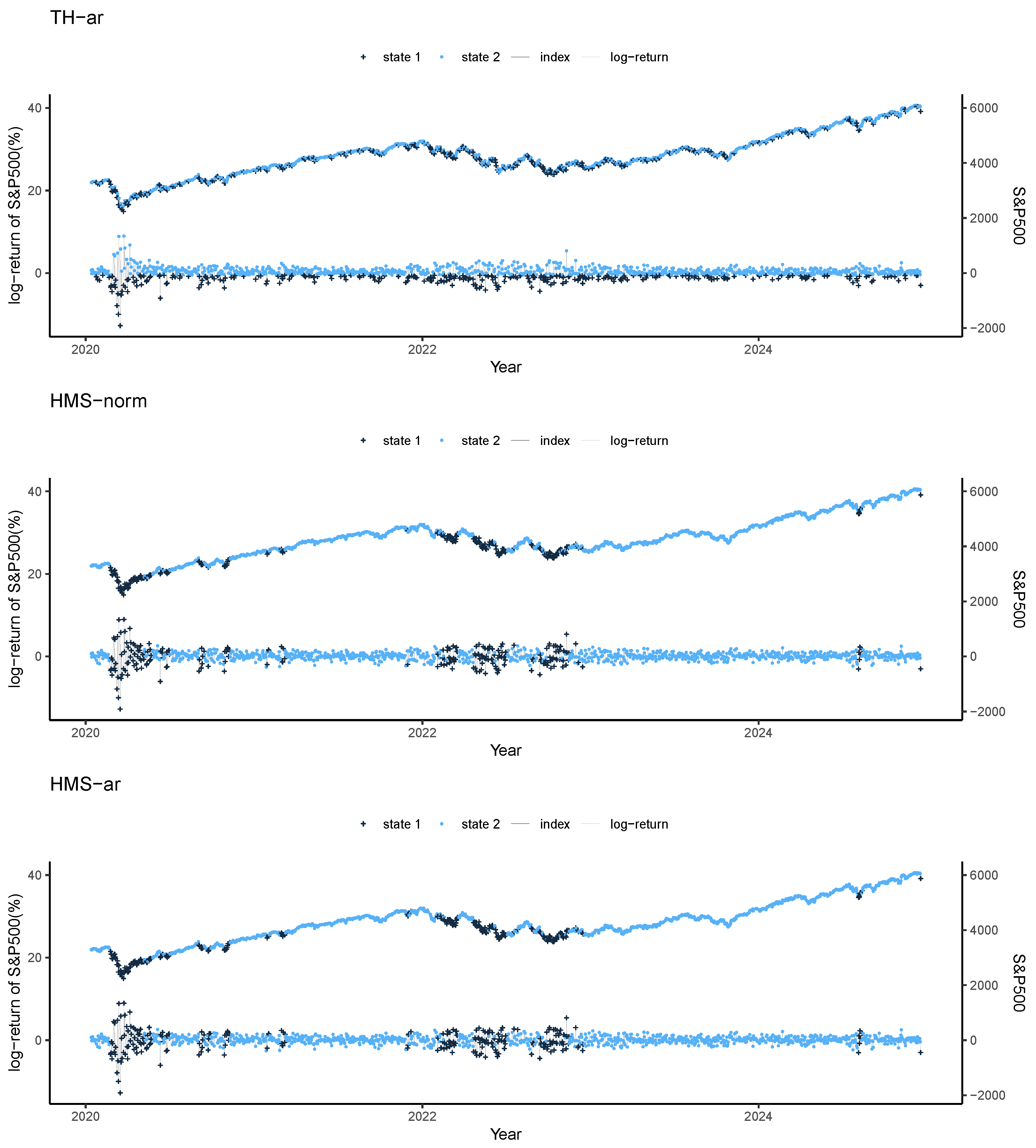
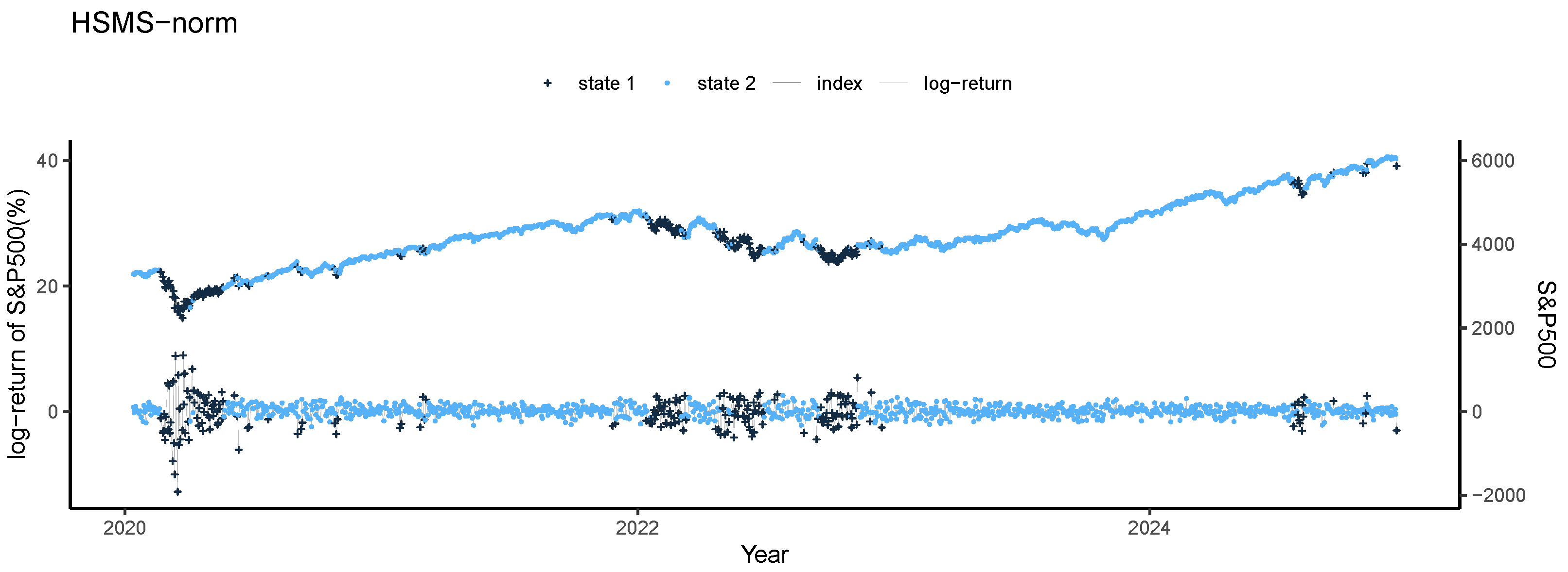
7.1. Example 1: The Daily Returns of the S&P 500

This subsection presents a real example comparing above six different regime switching models. We consider the daily log returns of the S&P 500 from 1 January 2020 to 27 December 2024, which contain 1255 observations. The original dataset is available at https://ca.investing.com/indices/us-spx-500-historical-data (accessed on 28 December 2024). This example illustrates the switching processes modeled by these six different regime switching approaches.

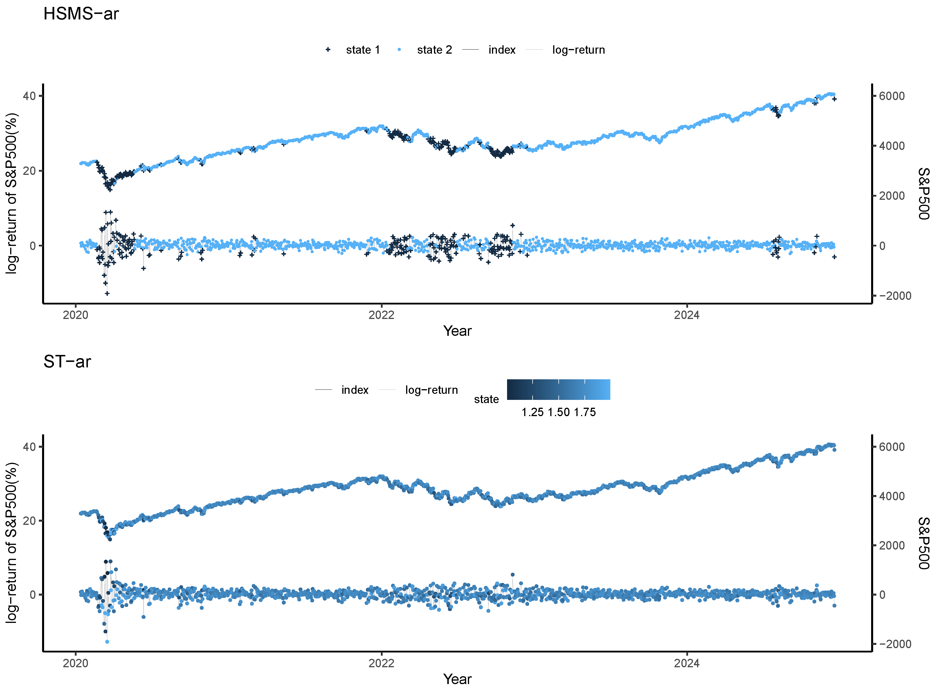
Figure 1 and Figure 2 visually depict the estimated regimes or states of the daily log returns of the S&P 500 via these six models. As discussed in Section 1, the TH-ar model aims to provide a local linear approximation to the underlying non-linear relationship, but it fails to capture regime switching behavior. The TH-ar model partitions the data based on an estimated threshold value of $\widehat{\tau }=-0.5226036$ that does not convey any information about the business cycle. In contrast, the HMS and HSMS models effectively identify bear and bull markets as States 1 and 2, respectively. By the similarity of the plots of the HMS-norm and HMS-ar in Figure 1, or HSMS-norm and HSMS-ar in Figure 2, the state-dependent structure has much less influence on state estimation compared with switching mechanisms. The ST-ar model provides a smooth transition between states, capturing the intermediate dynamics. In addition, the ST-ar model can represent the business cycle, with dark blue dots appearing around recession periods in the time series, indicating that the model aligns more closely with State 1 during these time periods.

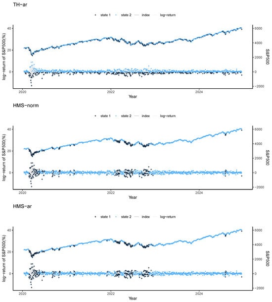
Figure 1. Estimation of the two states of the daily S&P 500 returns by TH-ar, HMS-norm, and HMS-ar: State 1 (dark blue “+”) and State 2 (light blue “•”). In each panel, the upper graph with black line is the daily S&P 500 returns with the estimated states (right axis), and the lower graph with grey line is the daily log-return of the S&P 500 with the estimated states (left axis).

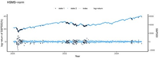
Figure 2. Estimation of the two states of the daily S&P 500 returns by the HSMS-norm, HSMS-ar, and ST-ar: State 1 (dark blue “+”) and State 2 (light blue “•”). In each panel, the upper graph with black line is the daily S&P 500 returns with the estimated states (right axis), and the lower graph with grey line is the daily log-return of the S&P 500 with the estimated states (left axis).

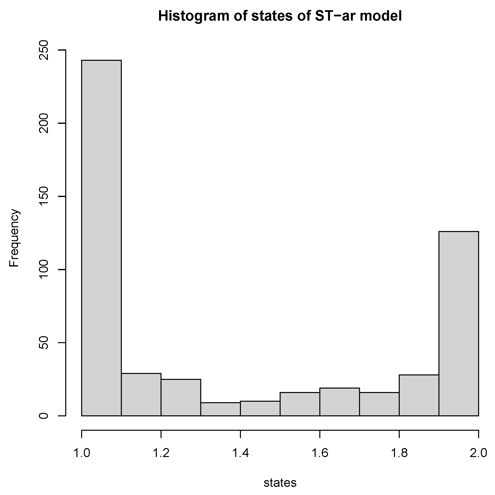
Table 1 provides the estimated parameters for each regime or state. State 1 represents depreciation periods with larger standard deviations and negative means. The TH-ar model exhibits slight differences in estimated parameters compared to the HMS and HSMS models. The HMS and HSMS exhibit more similar estimated parameters because HSMS model extends the HMS model by incorporating more flexible sojourn distributions. Both models are able to effectively capture regime switching behavior. The histogram of the state estimates by fitting the ST-ar model is displayed in Figure 3. Most estimated states fall within the range of 1.6 to 1.8. The state-dependent parameters of the ST-ar framework exhibit greater variability across states than those of the other models.

Table 1. Estimated parameters (${\widehat{\mu }}_i$) and standard deviations (${\widehat{\sigma }}_i$) of two-state regime switching models with state-dependent structure (21) for the daily S&P 500 returns (%). Estimated parameters ${\widehat{\alpha }}_i$ and ${\widehat{\varphi }}_{1,i}$ of two-state regime switching models with state-dependent structure (7) for the daily S&P 500 returns (%).

Method	${\widehat{\mathit{\mu }}}_1$	${\widehat{\mathit{\mu }}}_2$			${\widehat{\mathit{\sigma }}}_1$	${\widehat{\mathit{\sigma }}}_2$
HMS-norm	−0.26082	0.127168			2.517356	0.79785
HSMS-norm	−0.19689	0.108279			2.514641	0.835683
	${\widehat{\alpha }}_1$	${\widehat{\alpha }}_2$	${\widehat{\varphi }}_{1,1}$	${\widehat{\varphi }}_{1,2}$	${\widehat{\sigma }}_1$	${\widehat{\sigma }}_2$
TH-ar	−0.28359	0.185356	−0.27389	−0.28502	3.123607	1.272196
HMS-ar	−0.25524	0.113606	−0.27559	−0.01371	2.381922	0.827336
HSMS-ar	−0.29157	0.132293	−0.18612	−0.01109	2.409252	0.792376
ST-ar	−8.15227	3.774604	−1.27783	−1.01425

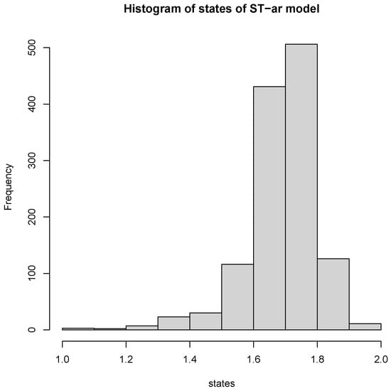
Figure 3. Histogram of the state estimates by fitting the ST-ar model for the daily S&P 500 returns (%).

Ref. [73] introduced the Akaike Information Criterion (AIC), one of the most popular model selection criteria, which is defined as follows:

$$\begin{array}{l}\hfill AIC=-2{\displaystyle \sum _{i=1}^n}lnf\left(x_i\right|\widehat{\theta })+2k,\end{array}$$

where k is the number of parameters, and ${\sum }_{i=1}^{n}lnf\left(x_i\right|\widehat{\theta })$ is the log-likelihood of the model with estimated parameters. Some studies have found that AIC is not consistent, especially in large samples.

Since AIC tends to select over-parameterized models ([74]), to address this issue, Ref. [75] introduced a consistent criterion for large samples, the Bayesian information criterion (BIC), which is based on a Bayesian framework and is given by

$$\begin{array}{l}\hfill BIC=-2{\displaystyle \sum _{i=1}^n}lnf\left(x_i\right|\widehat{\theta })+2kln\left(n\right),\end{array}$$

where k is the number of parameters, and ${\sum }_{i=1}^{n}lnf\left(x_i\right|\widehat{\theta })$ is the log-likelihood of the model with estimated parameters.

Table 2 compares the AIC and BIC of two-state regime switching models for the daily S&P 500 returns.The HMS-AR model performs best in terms of both AIC and BIC, with the best result highlighted in bold. The HSMS model performs better under AIC but worse than the TH-ar model under BIC because BIC imposes a larger penalty on model complexity.

Table 2. AIC and BIC of two-state regime switching models for the daily S&P 500 returns (%), with the best result highlighted in bold.

Method	AIC	BIC
HMS-norm	1693.650	1744.999
HSMS-norm	1812.655	2172.098
TH-ar	1923.529	1959.473
HMS-ar	1678.032	1739.651
HSMS-ar	1800.965	2170.677
ST-ar	5421.071	5457.015

7.2. Example 2: The Weekly Returns of the EURO STOXX 50

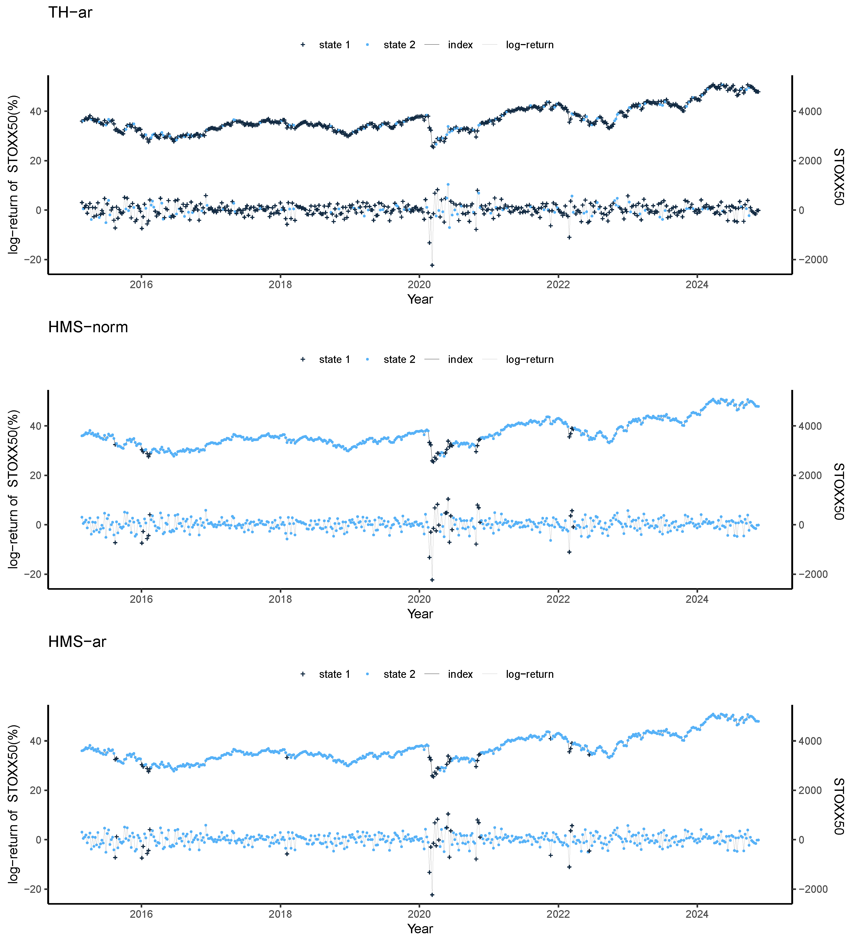
We estimate the two-state regime switching model for the weekly returns of EURO STOXX 50 spanning 1 January 2015, to 1 January 2025, using data available as of January 2025. The original dataset is from https://ca.investing.com/indices/eu-stoxx50-historical-data (accessed on 2 January 2025). Figure 4 and Figure 5 illustrate the states estimated using six different approaches. The TH-ar model fails to clearly distinguish between depreciation and appreciation periods, as evidenced by the overlap in the state assignments for States 1 and 2.

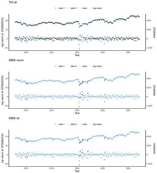
Figure 4. Estimation of the two states of the weekly EURO STOXX 50 index by TH-ar, HMS-norm, and HMS-ar: State 1 (dark blue “+”) and State 2 (light blue “•”). In each panel, the upper with black line graph is the weekly EURO STOXX 50 returns with the estimated states (right axis), and the lower graph with grey line is the weekly log-return of the EURO STOXX 50 with the estimated states (left axis).

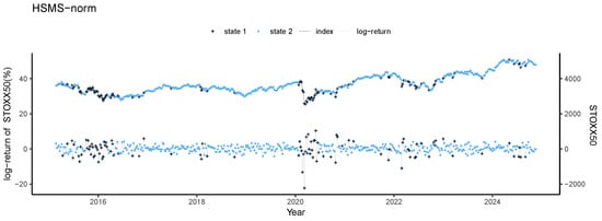
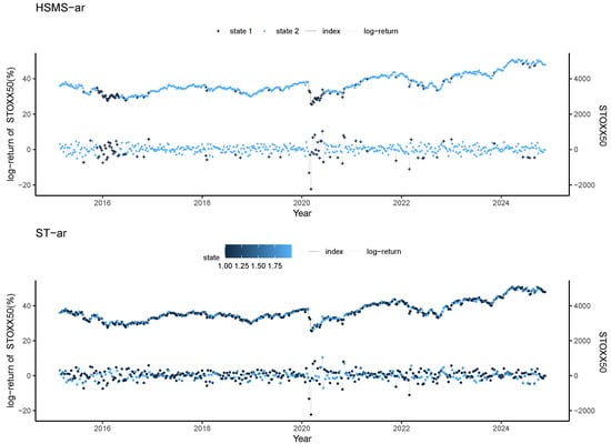
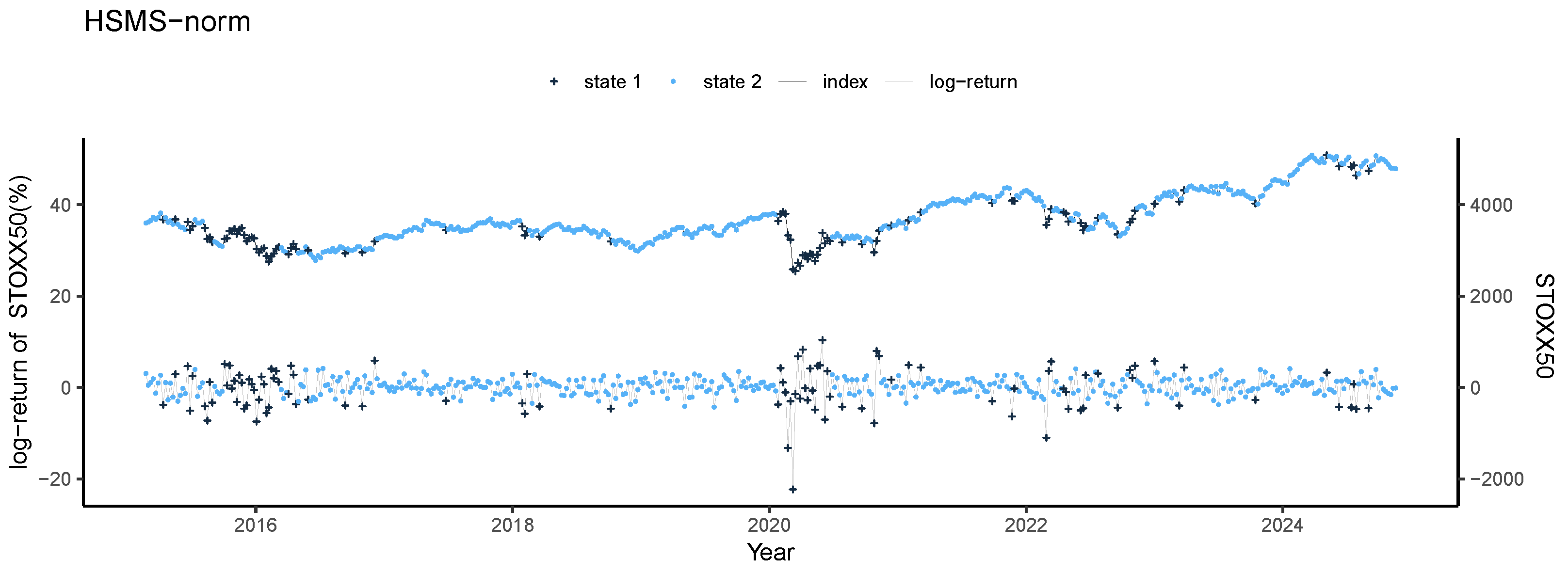
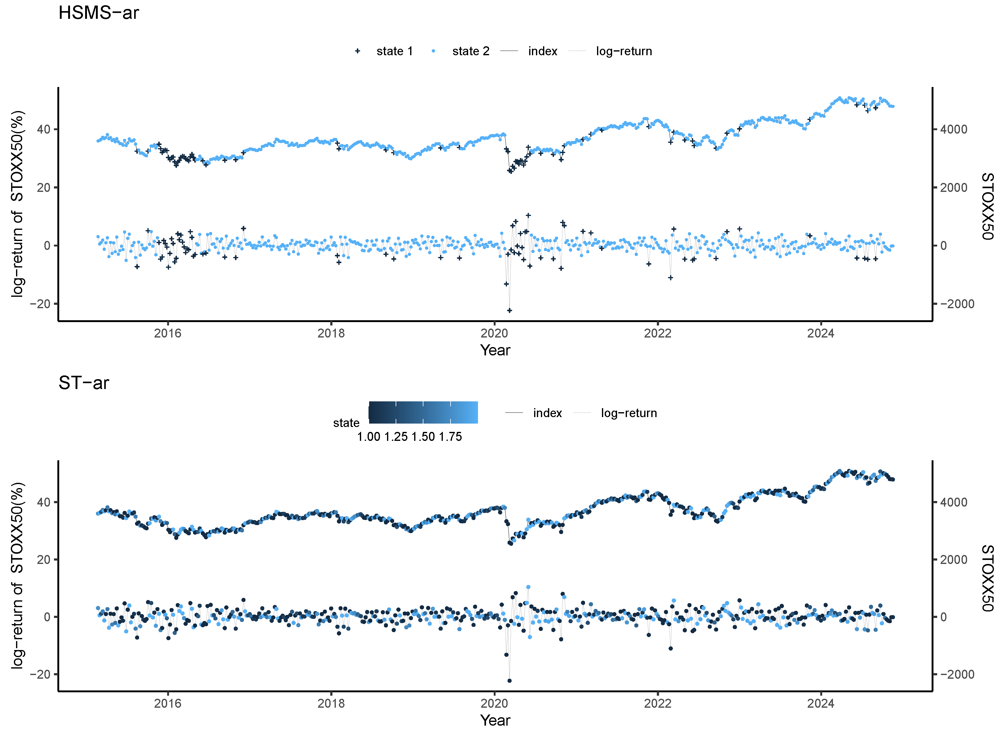
Figure 5. Estimation of the two states of the weekly EURO STOXX 50 index by the HSMS-norm, HSMS-ar, and ST-ar: State 1 (dark blue “+”) and State 2 (light blue “•”). In each panel, the upper graph with black line is the weekly EURO STOXX 50 returns with the estimated states (right axis), and the lower graph with grey line is the weekly log-return of the EURO STOXX 50 with the estimated states (left axis).

In contrast, the HMS and HSMS models successfully separated the two business phases, with the states showing more pronounced differences. These differences are even more distinct than those for the daily returns of the S&P 500. It is noteworthy that the HSMS model identifies a greater number of State 1, which can be attributed to its more flexible sojourn distribution. This flexibility suggests that, unlike the states estimated for the daily returns of the S&P 500, the sojourn distribution for the weekly returns of EURO STOXX 50 is not close to a geometric distribution.

The ST-ar model performs poorly, resulting in overlapping state estimates and thus no clear state separation can be achieved. The estimated parameters for all models are summarized in Table 3, while the histogram of the state estimates by fitting the ST-ar model to the EURO STOXX 50 returns is presented in Figure 6. The parameter estimates for HMS and HSMS models are similar, closely aligning with the results observed for the daily returns of the S&P 500. However, the state distribution by the ST-ar model for the weekly returns of EURO STOXX 50 is less concentrated than that of the daily returns of the S&P 500, where states are mainly located around 1 and 2.

Table 3. Estimated parameters (${\widehat{\mu }}_i$) and standard deviations (${\widehat{\sigma }}_i$) of two-state regime switching models with state-dependent structure (21) for the weekly EURO STOXX 50 returns (%). Estimated parameters ${\widehat{\alpha }}_i$ and ${\widehat{\varphi }}_{1,i}$ of two-state regime switching models with state-dependent structure (7) for the weekly EURO STOXX 50 index (%).

Method	${\widehat{\mathit{\mu }}}_1$	${\widehat{\mathit{\mu }}}_2$			${\widehat{\mathit{\sigma }}}_1$	${\widehat{\mathit{\sigma }}}_2$
HMS-norm	−0.41524	0.2549			4.498138	1.685982
HSMS-norm	−0.81259	0.162807			6.395816	2.095628
	${\widehat{\alpha }}_1$	${\widehat{\alpha }}_2$	${\widehat{\varphi }}_{1,1}$	${\widehat{\varphi }}_{1,2}$	${\widehat{\sigma }}_1$	${\widehat{\sigma }}_2$
TH-ar	−0.02741	0.23181	−0.0826	0.022965	7.404448	6.017856
HMS-ar	−0.8359	0.203724	0.080186	−0.11253	6.119401	2.042276
HSMS-ar	−0.65223	0.312221	0.148738	−0.19128	4.841668	1.735389
ST-ar	0.074356	0.120602	−0.15609	0.105752

Figure 6. Histogram of the state estimates by fitting the ST-ar model to the EURO STOXX 50 returns (%).

Table 4 compares the AIC and BIC of the two-state regime switching models for weekly EURO STOXX 50 returns. The HMS-ar model performs best according to the AIC, while the HMS-Norm model performs best according to the BIC, with the best result highlighted in bold. The HSMS model performs better under AIC, but underperforms the TH-ar model under BIC, as BIC imposes a larger penalty on model complexity.

Table 4. AIC and BIC of two-state regime switching models for the weekly EURO STOXX 50 returns (%), with the best result highlighted in bold.

Method	AIC	BIC
HMS-norm	2395.212	2447.77
HSMS-norm	2446.582	2814.484
TH-ar	2506.803	2543.593
HMS-ar	2392.059	2455.128
HSMS-ar	2433.276	2811.690
ST-ar	2511.391	2548.181

8. Conclusions

In this paper, we review four popular regime switching models, each defined by a different mechanism: threshold models, hidden Markov regime switching models, hidden semi-Markov models, and smooth transition models. For each type of switching mechanism, we review its relevant framework, popular models, and commonly used estimation methods. In addition, in Section 6, we introduce several emerging switching models that deserve further theoretical development and empirical investigation.

Furthermore, we compare six different regime switching models using two real data examples. The comparison considers different switching mechanisms and state-dependent structures. Threshold models aim to provide a local linear approximation of the underlying non-linear relationship. HMS and HSMS can better capture the business cycle dynamics compared to other models. In addition, HSMS features a more flexible sojourn distribution. Smooth transition models help achieve a smooth regime switching process. However, in some data applications, they may have difficulty in clearly separating the states.

References

- Contreras-Reyes, J.E. Information quantity evaluation of nonlinear time series processes and applications. Phys. D Nonlinear Phenom. 2023, 445, 133620. [Google Scholar]
- Tong, H. On a Threshold Model; Sijthoff & Noordhoff: Alphen aan den Rijn, The Netherlands, 1978. [Google Scholar]
- Hamilton, J.D. A new approach to the economic analysis of nonstationary time series and the business cycle. Econom. J. Econom. Soc. 1989, 57, 357–384. [Google Scholar]
- Zakoian, J.M. Threshold heteroskedastic models. J. Econ. Dyn. Control 1994, 18, 931–955. [Google Scholar]
- Freguson, J.D. Variable duration models for speech. In Symposium on the Application of Hidden Markov Models to Text and Speech; IDA-CRD: Princeton, NJ, USA, 1980; pp. 143–179. [Google Scholar]
- Amini, M.; Bayat, A.; Salehian, R. hhsmm: An R package for hidden hybrid Markov semi-Markov models. Comput. Stat. 2022, 38, 1283–1335. [Google Scholar]
- Teräsvirta, T. Specification, estimation, and evaluation of smooth transition autoregressive models. J. Am. Stat. Assoc. 1994, 89, 208–218. [Google Scholar]
- Liu, M.; Li, Q.; Zhu, F. Threshold negative binomial autoregressive model. Statistics 2019, 53, 1–25. [Google Scholar] [CrossRef]
- Liu, M.; Li, Q.; Zhu, F. Self-excited hysteretic negative binomial autoregression. AStA Adv. Stat. Anal. 2020, 104, 385–415. [Google Scholar]
- Yang, K.; Yu, X.; Zhang, Q.; Dong, X. On MCMC sampling in self-exciting integer-valued threshold time series models. Comput. Stat. Data Anal. 2022, 169, 107410. [Google Scholar]
- Yang, K.; Xu, N.; Li, H.; Zhao, Y.; Dong, X. Multivariate threshold integer-valued autoregressive processes with explanatory variables. Appl. Math. Model. 2023, 124, 142–166. [Google Scholar]
- Tong, H.; Lim, K.S. Threshold autoregression, limit cycles and cyclical data. J. R. Stat. Soc. Ser. B (Methodol.) 1980, 42, 245–268. [Google Scholar] [CrossRef]
- Chen, C.W. A Bayesian analysis of generalized threshold autoregressive models. Stat. Probab. Lett. 1998, 40, 15–22. [Google Scholar] [CrossRef]
- Chen, C.W.; Chiang, T.C.; So, M.K. Asymmetrical reaction to US stock-return news: Evidence from major stock markets based on a double-threshold model. J. Econ. Bus. 2003, 55, 487–502. [Google Scholar]
- Chen, C.W.; So, M.K. On a threshold heteroscedastic model. Int. J. Forecast. 2006, 22, 73–89. [Google Scholar]
- Gerlach, R.; Chen, C.W.; Lin, D.S.; Huang, M.H. Asymmetric responses of international stock markets to trading volume. Phys. A Stat. Mech. Its Appl. 2006, 360, 422–444. [Google Scholar]
- Chen, R. Threshold variable selection in open-loop threshold autoregressive models. J. Time Ser. Anal. 1995, 16, 461–481. [Google Scholar]
- Wu, S.; Chen, R. Threshold variable determination and threshold variable driven switching autoregressive models. Stat. Sin. 2007, 17, 241-S38. [Google Scholar]
- Chen, C.W.; Liu, F.C.; So, M.K. A review of threshold time series models in finance. Stat. Its Interface 2011, 4, 167–181. [Google Scholar]
- Petruccelli, J.D.; Woolford, S.W. A threshold AR (1) model. J. Appl. Probab. 1984, 21, 270–286. [Google Scholar] [CrossRef]
- Chen, R.; Tsay, R.S. On the ergodicity of TAR (1) processes. Ann. Appl. Probab. 1991, 1, 613–634. [Google Scholar]
- Tong, H. Threshold Models in Non-Linear Time Series Analysis; Springer Science & Business Media: Berlin/Heidelberg, Germany, 2012; Volume 21. [Google Scholar]
- Chan, K.S.; Petruccelli, J.D.; Tong, H.; Woolford, S.W. A multiple-threshold AR (1) model. J. Appl. Probab. 1985, 22, 267–279. [Google Scholar]
- Chan, K.S.; Tong, H. On the use of the deterministic Lyapunov function for the ergodicity of stochastic difference equations. Adv. Appl. Probab. 1985, 17, 666–678. [Google Scholar]
- Ling, S.; Tong, H. Testing for a linear MA model against threshold MA models. Ann. Statist. 2005, 33, 2529–2552. [Google Scholar]
- Ling, S.; Tong, H.; Li, D. Ergodicity and invertibility of threshold moving-average models. Bernoulli 2007, 13, 161–168. [Google Scholar]
- Brockwell, P.J.; Liu, J.; Tweedie, R.L. On the existence of stationary threshold autoregressive moving-average processes. J. Time Ser. Anal. 1992, 13, 95–107. [Google Scholar]
- Ling, S. On the probabilistic properties of a double threshold ARMA conditional heteroskedastic model. J. Appl. Probab. 1999, 36, 688–705. [Google Scholar]
- Glosten, L.R.; Jagannathan, R.; Runkle, D.E. On the relation between the expected value and the volatility of the nominal excess return on stocks. J. Financ. 1993, 48, 1779–1801. [Google Scholar]
- Hagerud, G.E. A Smooth Transition ARCH Model for Asset Returns; SSE/EFI Working Paper Series in Economics and Finance,162; Stockholm School of Economics: Stockholm, Sweden, 1997. [Google Scholar]
- Gerlach, R.; Chen, C.W. Bayesian inference and model comparison for asymmetric smooth transition heteroskedastic models. Stat. Comput. 2008, 18, 391–408. [Google Scholar]
- Chen, C.W.; So, M.K.; Gerlach, R.H. Assessing and testing for threshold nonlinearity in stock returns. Aust. New Zealand J. Stat. 2005, 47, 473–488. [Google Scholar] [CrossRef]
- Chen, C.W.; Gerlach, R.; Lin, E.M. Volatility forecasting using threshold heteroskedastic models of the intra-day range. Comput. Stat. Data Anal. 2008, 52, 2990–3010. [Google Scholar]
- Chen, C.W.; Gerlach, R.H.; Lin, A.M. Falling and explosive, dormant, and rising markets via multiple-regime financial time series models. Appl. Stoch. Model. Bus. Ind. 2010, 26, 28–49. [Google Scholar] [CrossRef]
- Li, C.W.; Li, W.K. On a double-threshold autoregressive heteroscedastic time series model. J. Appl. Econom. 1996, 11, 253–274. [Google Scholar] [CrossRef]
- Brooks, C. A double-threshold GARCH model for the French Franc/Deutschmark exchange rate. J. Forecast. 2001, 20, 135–143. [Google Scholar] [CrossRef]
- Chen, C.W.; Gerlach, R.H.; Lin, A.M. Multi-regime nonlinear capital asset pricing models. Quant. Financ. 2011, 11, 1421–1438. [Google Scholar] [CrossRef]
- Audrino, F.; Bühlmann, P. Tree-structured generalized autoregressive conditional heteroscedastic models. J. R. Stat. Soc. Ser. B Stat. Methodol. 2001, 63, 727–744. [Google Scholar] [CrossRef]
- So, M.K.; Li, W.K.; Lam, K. A threshold stochastic volatility model. J. Forecast. 2002, 21, 473–500. [Google Scholar] [CrossRef]
- Chen, C.W.; Liu, F.C.; So, M.K. Heavy-tailed-distributed threshold stochastic volatility models in financial time series. Aust. New Zealand J. Stat. 2008, 50, 29–51. [Google Scholar] [CrossRef]
- Ghaddar, D.K.; Tong, H. Data transformation and self-exciting threshold autoregression. J. R. Stat. Soc. Ser. C Appl. Stat. 1981, 30, 238–248. [Google Scholar] [CrossRef]
- Hamilton, J.D.; Susmel, R. Autoregressive conditional heteroskedasticity and changes in regime. J. Econom. 1994, 64, 307–333. [Google Scholar] [CrossRef]
- Baum, L.E.; Eagon, J.A. An inequality with applications to statistical estimation for probabilistic functions of Markov processes and to a model for ecology. Bull. Amer. Math. Soc. 1967, 73, 360–363. [Google Scholar] [CrossRef]
- Medhioub, I. A Markov switching three regime model of Tunisian business cycle. Am. J. Econ. 2015, 5, 394–403. [Google Scholar]
- Ayodeji, I.O. A Three-State Markov-Modulated Switching Model for Exchange Rates. J. Appl. Math. 2016, 2016, 5061749. [Google Scholar] [CrossRef]
- Gray, S.F. Modeling the conditional distribution of interest rates as a regime-switching process. J. Financ. Econ. 1996, 42, 27–62. [Google Scholar] [CrossRef]
- Krolzig, H.M. Econometric Modelling of Markov Switching Vector Auto-Regressions Using MSVAR for Ox; Discussion Paper; Department of Economics, University of Oxford: Oxford, UK, 1998. [Google Scholar]
- So, M.E.P.; Lam, K.; Li, W.K. A stochastic volatility model with Markov switching. J. Bus. Econ. Stat. 1998, 16, 244–253. [Google Scholar] [CrossRef]
- Hardy, M.R. Regime-Switching Model of Long-Term Stock Returns. N. Am. Actuar. J. 2001, 5, 41–53. [Google Scholar] [CrossRef]
- Shi, Y.; Ho, K.Y. Long memory and regime switching: A simulation study on the Markov regime-switching ARFIMA model. J. Bank. Financ. 2015, 61, S189–S204. [Google Scholar] [CrossRef]
- Ma, F.; Wahab, M.I.M.; Huang, D.; Xu, W. Forecasting the realized volatility of the oil futures market: A regime switching approach. Energy Econ. 2017, 67, 136–145. [Google Scholar] [CrossRef]
- Augustyniak, M. Maximum likelihood estimation of the Markov switching GARCH model. Comput. Stat. Data Anal. 2014, 76, 61–75. [Google Scholar] [CrossRef]
- Amisano, G.; Fagan, G. Money growth and inflation: A regime switching approach. J. Int. Money Financ. 2013, 33, 118–145. [Google Scholar] [CrossRef]
- Kim, C.-J.; Nelson, C.R. State-Space Models with Regime Switching Classical and Gibbs Sampling Approaches with Applications; MIT Press: Cambridge, MA, USA, 1999. [Google Scholar]
- Francq, C.; Zakoı, J.M. Deriving the autocovariances of powers of Markov switching GARCH models, with applications to statistical inference. Comput. Stat. Data Anal. 2008, 52, 3027–3046. [Google Scholar] [CrossRef]
- Zheng, K.; Li, Y.; Xu, W. Regime switching model: Spectral clustering hidden Markov model. Ann. Oper. Res. 2021, 303, 297–319. [Google Scholar]
- Maruotti, A.; Petrella, L.; Sposito, L. Hidden semi-Markov switching quantile regression for time series. Comput. Stat. Data Anal. 2021, 159, 107208. [Google Scholar] [CrossRef]
- Bulla, J.; Bulla, I. Stylized facts of financial time series and hidden semi-Markov models. Computational statistics & data analysis 2006, 51, 2192–2209. [Google Scholar]
- Maruotti, A.; Punzo, A.; Bagnato, L. Hidden Markov and semi-Markov models with multivariate leptokurtic-normal components for robust modeling of daily returns series. J. Financ. Econom. 2019, 17, 91–117. [Google Scholar] [CrossRef]
- Yu, S.Z. Hidden semi-Markov models. Artif. Intell. 2010, 174, 215–243. [Google Scholar] [CrossRef]
- Balcilar, M.; Gupta, R.; Miller, S.M. Regime switching model of US crude oil and stock market prices: 1859 to 2013. Energy Econ. 2015, 49, 317–327. [Google Scholar]
- Xiao, S.; Dong, M. Hidden semi-Markov model-based reputation management system for online to offline (O2O) e-commerce markets. Decis. Support Syst. 2015, 77, 87–99. [Google Scholar]
- Bernardi, M.; Maruotti, A.; Petrella, L. Multivariate Markov Switching models and tail risk interdependence. arXiv 2018, arXiv:1312.6407v3. [Google Scholar]
- Qin, S.; Tan, Z.; Wu, Y. On robust estimation of hidden semi-Markov regime-switching models. Ann. Oper. Res. 2024, 338, 1049–1081. [Google Scholar]
- Eitrheim, Ø.; Teräsvirta, T. Testing the adequacy of smooth transition autoregressive models. J. Econom. 1996, 74, 59–75. [Google Scholar]
- Michael, P.; Nobay, A.R.; Peel, D.A. Transactions costs and nonlinear adjustment in real exchange rates; An empirical investigation. J. Political Econ. 1997, 105, 862–879. [Google Scholar]
- Baum, C.F.; Barkoulas, J.T.; Caglayan, M. Nonlinear adjustment to purchasing power parity in the post-Bretton Woods era. J. Int. Money Financ. 2001, 20, 379–399. [Google Scholar]
- Jansen, E.S.; Teräsvirta, T. Testing parameter constancy and super exogeneity in econometric equations. Oxf. Bull. Econ. Stat. 1996, 58, 735–763. [Google Scholar]
- Chang, Y.; Choi, Y.; Park, J.Y. A new approach to model regime switching. J. Econom. 2017, 196, 127–143. [Google Scholar]
- Bazzi, M.; Blasques, F.; Koopman, S.J.; Lucas, A. Time-varying transition probabilities for Markov regime switching models. J. Time Ser. Anal. 2017, 38, 458–478. [Google Scholar]
- Li, D.; Ling, S. On the least squares estimation of multiple-regime threshold autoregressive models. Journal of Econometrics 2012, 167, 240–253. [Google Scholar]
- van Dijk, D. Smooth Transition Models: Extensions and Outlier Robust Inference. Ph.D. Thesis, Erasmus Universiteit Rotterdam, Rotterdam, The Netherlands, 1999. [Google Scholar]
- Akaikei, H. Information theory and an extension of maximum likelihood principle. In Proceedings of the 2nd International Symposium on Information Theory, Tsahkadsor, Armenia, 2–8 September 1973; pp. 267–281. [Google Scholar]
- Shibata, R. Selection of the order of an autoregressive model by Akaike’s information criterion. Biometrika 1976, 63, 117–126. [Google Scholar] [CrossRef]
- Schwarz, G. Estimating the Dimension of a Model. Ann. Stat. 1978, 6, 461–464. [Google Scholar] [CrossRef]
Disclaimer/Publisher’s Note: The statements, opinions and data contained in all publications are solely those of the individual author(s) and contributor(s) and not of MDPI and/or the editor(s). MDPI and/or the editor(s) disclaim responsibility for any injury to people or property resulting from any ideas, methods, instructions or products referred to in the content. |
© 2025 by the authors. Licensee MDPI, Basel, Switzerland. This article is an open access article distributed under the terms and conditions of the Creative Commons Attribution (CC BY) license (https://creativecommons.org/licenses/by/4.0/).