Abstract
The study of algebraic invariants associated with Brauer configuration algebras induced by appropriate multisets is said to be a Brauer analysis of the data that define the multisets. In general, giving an explicit description of such invariants as the dimension of the algebras or the dimension of their centers is a hard problem. This paper performs a Brauer analysis on some generators of Thompson’s group F. It proves that such generators and some appropriate Christoffel words induce Brauer configuration algebras whose dimensions are given by the number of edges and vertices of the binary trees defining them. The Brauer analysis includes studying the covering graph induced by a corresponding quiver; this paper proves that these graphs allow for finding set-theoretical solutions of the Yang–Baxter equation.
Keywords:
Brauer configuration algebra; Brauer analysis; Christoffel word; path algebra; Thompson’s group; Yang–Baxter equation MSC:
16G20; 16G30; 16G60; 16T25; 20F65
1. Introduction
Thompson’s groups, or Chameleon groups, were introduced by Thompson in some unpublished handwritten notes in 1965. They are a family of finitely presented infinite groups denoted F, T, and V such that . Thompson proved that groups T and V are simple. His original goal was to model certain concepts of logic, and later on, it was noticed that F, T, and V could be realized as subgroups of the groups of piecewise linear homeomorphisms [1] of the unit interval, the circle, and the Cantor set, respectively. They have also been studied as groups of isomorphisms of rooted binary trees [2]. Additional historical remarks regarding the seminal ideas of Thompson and Higman on the construction of these groups can be found in [3].
Thompson’s groups have played an important role in different fields of mathematics and computer sciences. For instance, they have been used to study the solvability of the word problem [4], the homotopy theory [5], the Teichmüller theory [6], and dynamic data storage in trees [7].
Recently, several connections have been found between Thompson’s group theory and cluster algebras theory via the rotation distance problem [8] and the Catalan combinatorics realized by binary trees, Dyck paths, and polygon triangulations [9].
The theory of Brauer configuration algebras introduced by Green and Schroll [10] is another example of a theory that has a role in different fields of mathematics and sciences. These algebras are path algebras defined by an appropriate collection of multisets. The study of their algebraic invariants as their dimensions and the structure of their indecomposable projective modules or their centers is said to be a Brauer analysis or a Brauer data analysis [11].
Brauer analysis has been applied to study several cybersecurity topics [12], graph entropy, and quantum entanglement states [11].
The Yang–Baxter equation (YBE) arose from theoretical physics and statistical mechanics research. Yang [13] introduced in 1967 such an equation in two short papers regarding generalizations of the results obtained by Lieb and Liniger [14]. On the other hand, Baxter [15] solved the eight-vertex ice model in 1971, which Lieb [16] had previously introduced. Baxter’s method was based on commuting transfer matrices starting from a solution he called the generalized star–triangle equation, which nowadays is known as the Yang–Baxter equation [17]. It is worth pointing out that finding a complete classification of the YBE solutions remains an open problem.
Relationships between quantum computing, the Yang–Baxter equation, Thompson’s groups, and the theories of knots and braids have been intensively studied in the last few years. On the one hand, anyonic systems allowed for finding quantum algorithms to evaluate Jones polynomials [18], which are topological invariants of knots and links [19]. Dehornoy [20] established relationships between Thompson’s group F and the braid group . Particularly, it is well-known that generators of satisfy the Yang–Baxter equation. We also remember that Jones [21] studied unitary representations of Thompson’s group F and defined a method to construct knots and links from such group F.
Connections between Thompson’s group theory, the Yang–Baxter equation, and the theory of Brauer configuration algebras were also explored by Cañadas et al. in [22]. In this work, the authors gave set-theoretical solutions to the Yang–Baxter equation by defining some algebraic structures called braces by Rump [23]. It is worth noting that braces have been systematically used to solve different versions of the Yang–Baxter equation [24].
This paper gives a novel perspective of the interplay between Thompson’s groups, Brauer analysis, and the Yang–Baxter equation. It applies Brauer analysis to some generators of Thompson’s group F. It uses their corresponding covering graphs (which are part of the tools to be analyzed in the associated Brauer analysis [25]) to define some set-theoretical solutions of the Yang–Baxter-equation.
Contributions
This paper provides an extended Brauer analysis of some generators of Thompson’s group F and uses it to give set-theoretical solutions of the Yang–Baxter equation. Its main results are Theorems 1–9.
Theorem 1 gives a formula for the center dimension of a Brauer configuration algebra of type M. Theorem 2 states that Brauer configuration algebras induced by binary trees obtained via tree rotation are isomorphic. Theorem 3 gives examples of isomorphic Brauer configuration algebras induced by some Brauer configurations of type M, which can be realized as binary trees.
Theorem 4 applies an extended Brauer analysis to some generators of Thompson’s group F. Theorem 5 describes paths (in the rotation graph) connecting binary trees defined by the domain and range of some generators of Thompson’s group F.
Theorem 6 gives formulas for the dimension of Brauer configuration algebras induced by-products of Thompson’s group F generators. Theorem 7 describes the structure of covering graphs induced by generators of Thompson’s group F.
Theorem 8 provides set-theoretical solutions of the Yang–Baxter equation based on covering graphs induced by Thompson’s group F generators. Theorem 9 gives formulas for the dimensions of Brauer configuration algebras, their centers, and covering graphs induced by Christoffel words defined by Thompson’s group generators.
2. Preliminaries
This section gives basic definitions and notation regarding Thompson’s groups, Brauer configuration algebras, and the Yang–Baxter equation.
2.1. Background
A Brauer data analysis studies algebraic and combinatorial invariants associated with Brauer configuration algebras. Green and Schroll introduced Brauer configuration algebras [10] and Brauer graph algebras [26] to investigate algebras of tame and wild representation types.
Green and Schroll [10] gave formulas for the dimension of a Brauer configuration algebra induced by an appropriate system of multisets called Brauer configurations. Afterward, Espinosa et al. [27] defined Brauer messages and their specializations, which were used to realize problems in different fields of mathematics and sciences in terms of Brauer messages.
Cañadas et al. [12] found relationships between cybersecurity and Brauer analysis, which were also used to describe some quantum entangled states [11]. In particular, they explored relationships between Thompson’s group F, Yang–Baxter equations, and Brauer messages in [22].
Initially, Brauer analysis used dimensions of Brauer configuration algebras and their centers to analyze the underlying data without paying attention to the associated topological content information. Cañadas et al. [25] filled this gap by introducing the notion of entropy of a Brauer configuration and the covering graph. They used these tools and some degree-based entropies to analyze Dynkin and Euclidean diagrams.
This paper applies Brauer analysis to appropriate generators of Thompson’s group F. Particularly, we will see that corresponding covering graphs can be used to provide set-theoretical solutions of the Yang–Baxter equation.
2.2. Thompson’s Group F
This section reminds definitions and notations regarding Thompson’s group F.
Any subdivision of the interval into dyadic intervals of the form , is a dyadic division of .
If , are dyadic subdivisions with the same number of cuts, then it is possible to define a piecewise-linear homeomorphism by sending each interval of linearly onto the corresponding interval in . This is called a dyadic rearrangement of . In such a case, all the slopes of f are powers of 2, and all the breakpoints of f have dyadic rational coordinates.
The set F of all dyadic rearrangements forms a group under composition called Thompson’s group F [28].
Any element of F can be described by a pair of finite binary trees with the same number of leaves, where each leaf of a tree represents an interval of the subdivision and the root represents the interval , the other nodes represent intervals from intermediate stages of the dyadic subdivision. The element of F is found by mapping linearly the corresponding intervals to the leaves, in an order-preserving fashion.
Two dyadic subdivisions of always have a common subdivision. That is, given two binary trees, there is the least common multiple, i.e., a unique minimal tree that contains both [29].
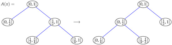
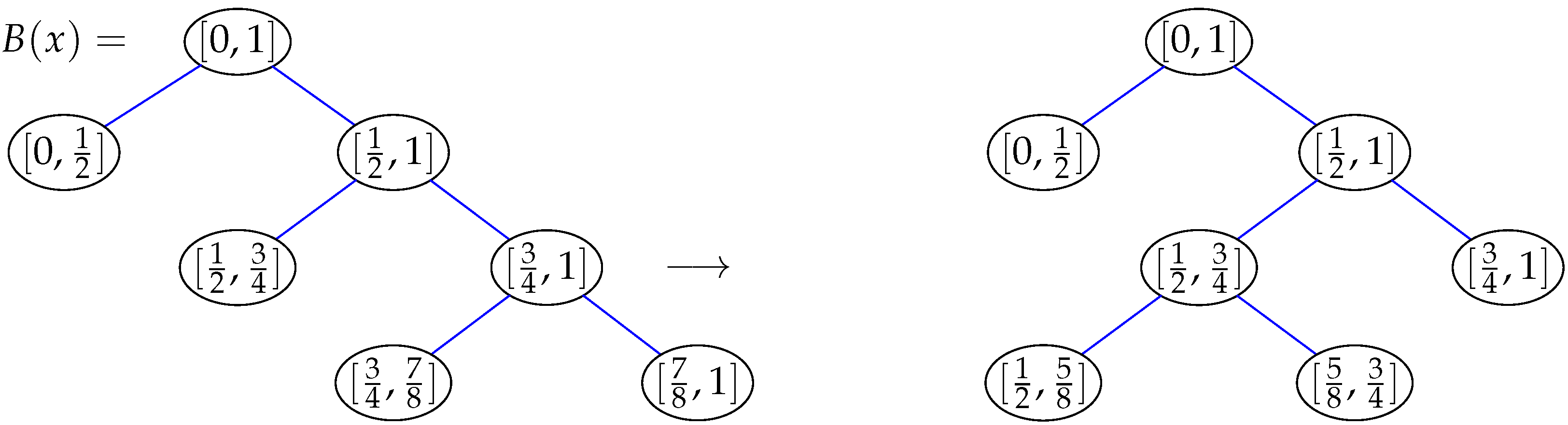
Figure 1.
A pair of binary trees represent generator of Thompson’s group F.
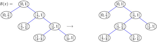
Figure 2.
A pair of binary trees with four leaves represent generator of Thompson’s group F.
A caret in a finite binary tree T is a subgraph of T, which has as a set of vertices , where is a fixed vertex , whereas and are the children of . The caret has the sets and as the only edges. Two elements of F are equivalent if there is a sequence of additions and reductions in carets transforming one into the other. A binary tree with no reducible carets is said to be reduced.
If , and are binary trees and , then the composition is represented by a tree product of the form , which can be realized by finding the least common multiple R of and S, which will play the role of the middle interval in the composition. Find then two representatives for the two elements of the form and [29]. The product element is then represented by the pair tree (see Figure 3).
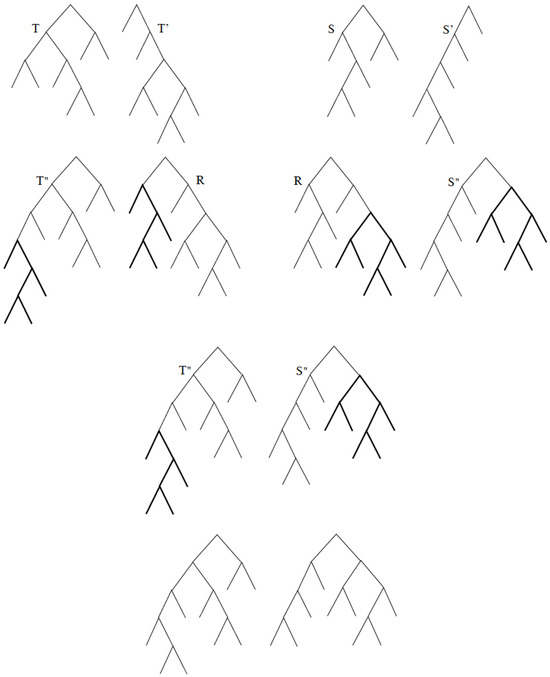
Figure 3.
Example of a composition in Thompson’s group F [29].
The following is a presentation of the group F in terms of generators and [30]:
An infinite presentation of F is given as follows:
where and for , it holds that .
Thompson’s group F satisfies the following properties [30]:
- F is torsion-free, contains free semi-group on two generators, and contains no nonabelian free group.
- Every subgroup of F is finite rank free abelian or contains an infinite rank free abelian subgroup.
- Every proper quotient of F is abelian.
- is simple and .
2.3. Tree Operations
Tree operations are used in the context of dynamic tree problems. For instance, Sleator and Tarjan [7] introduced three kinds of operations (, , and ) to represent trees using a data structure that allowed them to easily extract certain information about the trees and easily update the structure to reflect changes caused by such operations.
- is defined in such a way that if v is a tree root and w is a vertex in another tree, link the trees containing v and w by adding the edge , making w the parent of v.
- divides a given rooted tree into two new trees by deleting the edge from a vertex v (which is not a tree root) to its parent.
- turns a tree containing a vertex v inside out by making v the root of the tree.
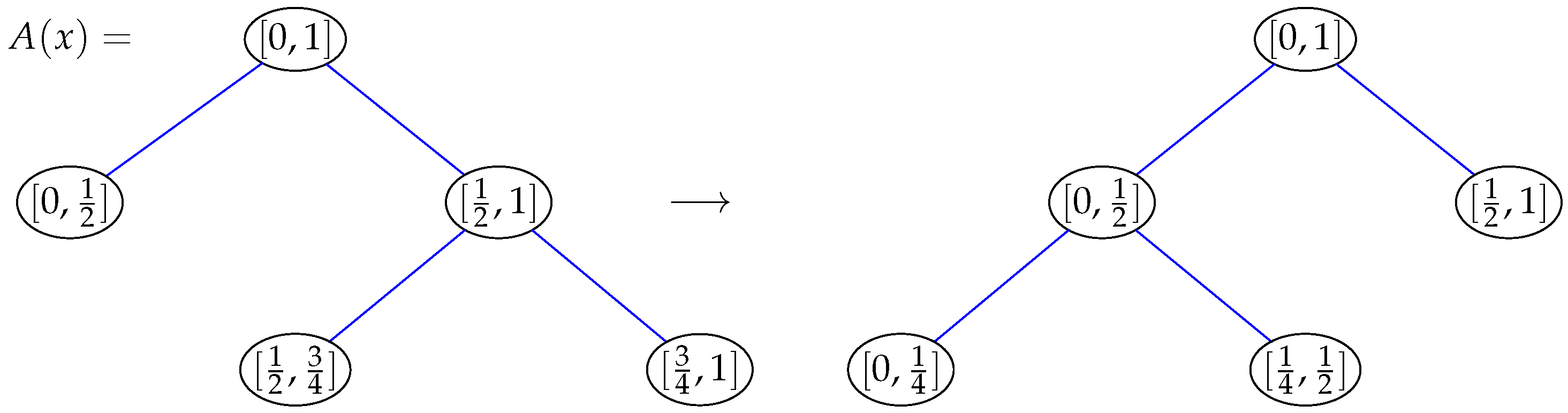
A rotation in a binary tree is obtained by collapsing an internal edge (external nodes have no children) of the tree to a point, thereby obtaining a node with three children, and then re-expanding the node of order three in the alternative way into two nodes of order two [8]. Any binary tree of size n can be converted into any other by performing an appropriate sequence of rotations.
The rotation graph for trees of size n is an undirected graph with one vertex for each tree of size n and an edge between vertices T and if there is a rotation that changes T into .
The main problem regarding rotation graphs is estimating their diameter, i.e., the maximum rotation distance between any two n-node binary trees. The rotation of a tree T with respect to a vertex a is denoted by .
Example 1.
Binary trees shown in Figure 1 are obtained by rotating one into the other. In such a case, if () denotes the binary tree associated with the domain (range) of , then and
2.4. Yang–Baxter Equation and Its Solutions
This section reminds the definition of the Yang–Baxter equation and some well-known methods for solving it.
Let V be a vector space over an algebraically closed field k of characteristic zero. A linear automorphism R of is a solution of the Yang–Baxter equation (sometimes called the braided relation) if the following identity (3) holds:
in the automorphism group .
R is a solution of the quantum Yang–Baxter equation if and only if
where means R acting on the ith, jth tensor factor and as the identity on the remaining factor [31].
To date, finding a complete classification of all the solutions of the YBE is an open problem. However, several approaches have been explored to obtain solutions of these equations. For instance, Drinfeld et al. [32] proposed studying set-theoretical solutions to the YBE; in such a case, for a given set X and a map , the identity (3) has the form [33]
where the maps are defined as , .
Note that, if is defined in such a way that , then a map is a set-theoretical solution of the YBE if and only if and satisfy the quantum Yang–Baxter Equation (4) [34,35].
A bijective map , such that is involutive if . r is said to be left non-degenerate (right non-degenerate) if each map () is bijective.
Note that, if X is finite, then an involutive solution of the braided equation is right non-degenerate if and only if it is left non-degenerate. It is worth noticing that non-degenerate involutive set-theoretical solutions of the YBE have been given by Etingof et al. [36] and Gateva-Ivanova and Van den Bergh [37] by associating a group to the solution .
Rump [23] introduced another line of investigation to tackle the problem of classifying the non-degenerate involutive set theoretical solutions of the YBE. To do that, he defined right braces and left braces. A right brace is a set G with two operations + and · such that
- is an abelian group;
- is a group.
is said to be the additive group and the multiplicative group of the right brace.
A left brace is defined similarly; in this case, the identity (6) has the shape
For , we define (the symmetric group on G) by
Rump proved the following result.
Lemma 1
(Lemma 4.1, [24], Propositions 2 and 3 [23]). Let G be a left brace. The following properties hold.
- 1.
- .
- 2.
- .
- 3.
- The map defined by is a non-degenerate involutive set-theoretical solution of the YBE.
Recently, Guarnieri and Vendramin [38] generalized Rump’s work to the noncommutative setting in order to obtain not necessarily non-degenerate involutive set-theoretical solutions of the YBE. Whereas, Ballester-Bolinches et al. [33] endowed a subgroup (of the symmetric group ) associated with a solution of the YBE with two operations + and · in such a way that the algebraic structure is a left brace. To do that, they used the Cayley graph of .
This paper introduces operations between binary trees representing Thompson’s group F generators to construct set-theoretical solutions of the Yang–Baxter equation.
2.5. Multisets and Brauer Configuration Algebras
This section provides definitions regarding multisets and their applications in the theory of Brauer configuration algebras. The authors refer interested readers to [10,25,39] for more insights about these subjects.
A multiset is a pair consisting of a set M and a map from M to the set of nonnegative integers . Note that a multiset allows element repetition [39]. In such a case, if , then is the multiplicity of m in M, which gives the number of occurrences of . The multiplicity function defines an expansion of the multiset M, which is a chain or linear order with the following form [10]:
If , then the word determined by is a fixed permutation of the elements or letters contained in M including repetitions. Note that has the following form:
In particular, it is possible to assume that .
If the set of letters M is such that , then a collection or set of multisets is said to be of type M if the following conditions hold [25]:
- Each letter has associated a linear ordered set or successor sequence , where , is the collection of all multisets containing m and , with , and , , if .
- If is the size of the multiset , then , .
- There exists a map ) such that , where is said to be the valency of m. If and (), then (). In particular, the successor sequence associated with m is , if .
Note that the successor sequence has the following form:
Each successor sequence can be extended to a circular ordering by adding a relation of the form . Such completion defines equivalent circular orderings as the following:
If denotes the successor of a multiset in some successor sequence , then it holds that
Collections of multisets of type M define Brauer configurations in the sense of Green and Schroll [10], where for each , it holds that and is an orientation given by the successor sequences . Green and Schroll called vertices (polygons) the elements of M ().
The product associated with the map of a Brauer configuration of type M allows for classifying the letters or vertices of the set M as truncated, in which case or nontruncated if . Note that, by definition, vertices or letters in Brauer configurations of type M are nontruncated.
The Brauer quiver (or simply Q if no confusion arises) induced by a collection of multisets of type M (or a Brauer configuration of type M) is a directed graph whose set of vertices is in bijective correspondence with the set (or collection) of polygons . Furthermore, if for some , where is the successor , then there exists an arrow such that and . Moreover, any circular ordering gives rise to a cycle (special cycle) contained in [25].
The quiver defines a bound quiver algebra , generated by paths in and bounded by an admissible ideal generated by relations of the following types and :
- , if and are special cycles at vertices and contained in the same polygon . These are relations of type .
- , where is a special cycle at vertex and f is its first arrow. In particular, if is an arrow defined by with , then is a relation of this type provided that in such a case, is a special cycle at . These relations are said to be of type .
- , where and are arrows in defined by successor sequences and with , and . These relations are said to be of type .
Cañadas et al. [25] introduced the covering graph induced by a Brauer configuration , which has the set of polygons as the set of vertices and there exists an edge connecting two polygons if for some , there exists a successor sequence for which either or (in other words, provided that, for some , is a covering in the corresponding successor sequence ). We note that covering graphs have no multiple arrows or loops.
Given a subset of the set of vertices of a graph , a hair graph with respect to A is obtained from by attaching to each point , , a linear path with vertices.
Remark 1.
The following properties of Brauer configuration algebras were introduced by Green, Schroll [10], Sierra [40], and Cañadas et al. [25] (see [10] Theorem B, Proposition 2.7, Theorem 3.10, Corollary 3.12, [40] Theorem 4.9, and [25], Theorem 8).
- Any Brauer configuration algebra induced by a Brauer configuration is multiserial, and there exists a bijective correspondence between the set of indecomposable projective -modules and the set of multisets or polygons .
- The number of summands in the heart of an indecomposable projective -module equals the number of nontruncated vertices in the corresponding polygon. Where, () denotes the Jacobson radical (socle) of the indecomposable projective -module P.
- Green and Schroll [10] gave the following Formula (13) for the dimension of a Brauer configuration algebra induced by a Brauer configuration .
- Sierra [40] gave the following Formula (14) for the dimension of the center of a Brauer configuration algebra induced by a reduced and connected Brauer configuration (Brauer configurations of type M are reduced).
- We note that any graph gives rise to a Brauer configuration of type M, where and . Cañadas et al. [25] proved that the covering graph induced by a Brauer configuration defined by a graph is isomorphic to if and only if is a disjoint union of copies of connected hair graphs of type , where is an n-point cycle and .
Example 2.
Let us consider the generator of Thompson’s group F shown in Figure 1. We assume the following notation for vertices and edges of its domain and range:
For the domain, it is assumed the Brauer configuration is . Whereas, the Brauer configuration defined by the range of has the form . Where,
- , .
- .
- .
- , , .
- , , for the remaining vertices or letters.
- The Brauer configuration algebra induced by the Brauer configuration is indecomposable as an algebra, .
- Figure 4 shows Brauer quivers and . The following are examples of relations contained in the admissible ideal . Relations in are defined in the same fashion.
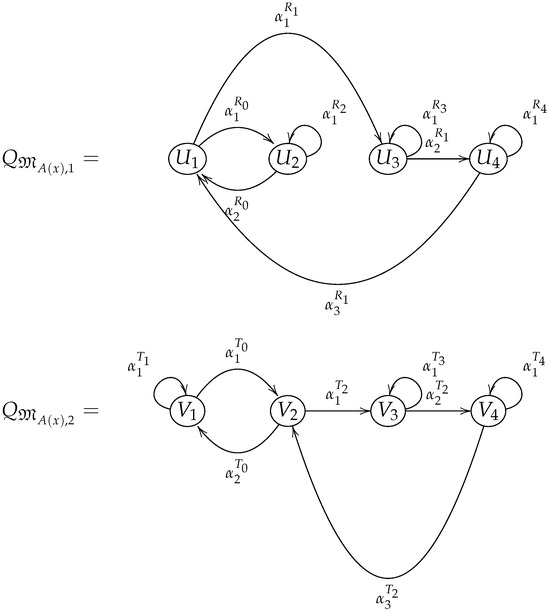 Figure 4. Brauer quivers induced by the generator (see Figure 1) of Thompson’s group F.
- 1.
- , , for all possible values of p and q.
- 2.
- , .
- 3.
- .
- 4.
- .
- 5.
- .
- 6.
- .
- 7.
- ; ; .
- For fixed, it holds that .
- and are isomorphic as algebras.
- is the Brauer configuration algebra induced by the generator of Thompson’s group F. Thus, .
- For fixed, it holds that . Note that there are three vertices with valency one and four polygons (see Formula (18)).
2.6. Entropy of a Graph
The entropy of a graph or network is a measure of its complexity; it was introduced by Rashevsky [41] and Trucco [42]. Cañadas et al. [25] studied based-degree graph entropies denoted , , and to apply extended Brauer analysis to some Dynkin and Euclidean diagrams. Such entropies are defined as follows for a graph and a Brauer configuration of type M induced by a graph .
where () denotes the set of vertices (edges) of a graph , denotes the number of vertices with degree equal to i and , is the degree of . Furthermore, .
Example 3.
Let be the binary tree defined by the domain of Thompson’s group F generator (see Figure 1); then,
The following Example 4 gives an extended Brauer analysis of a hair graph of type , where denotes a three-point cycle.
Example 4.
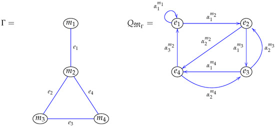
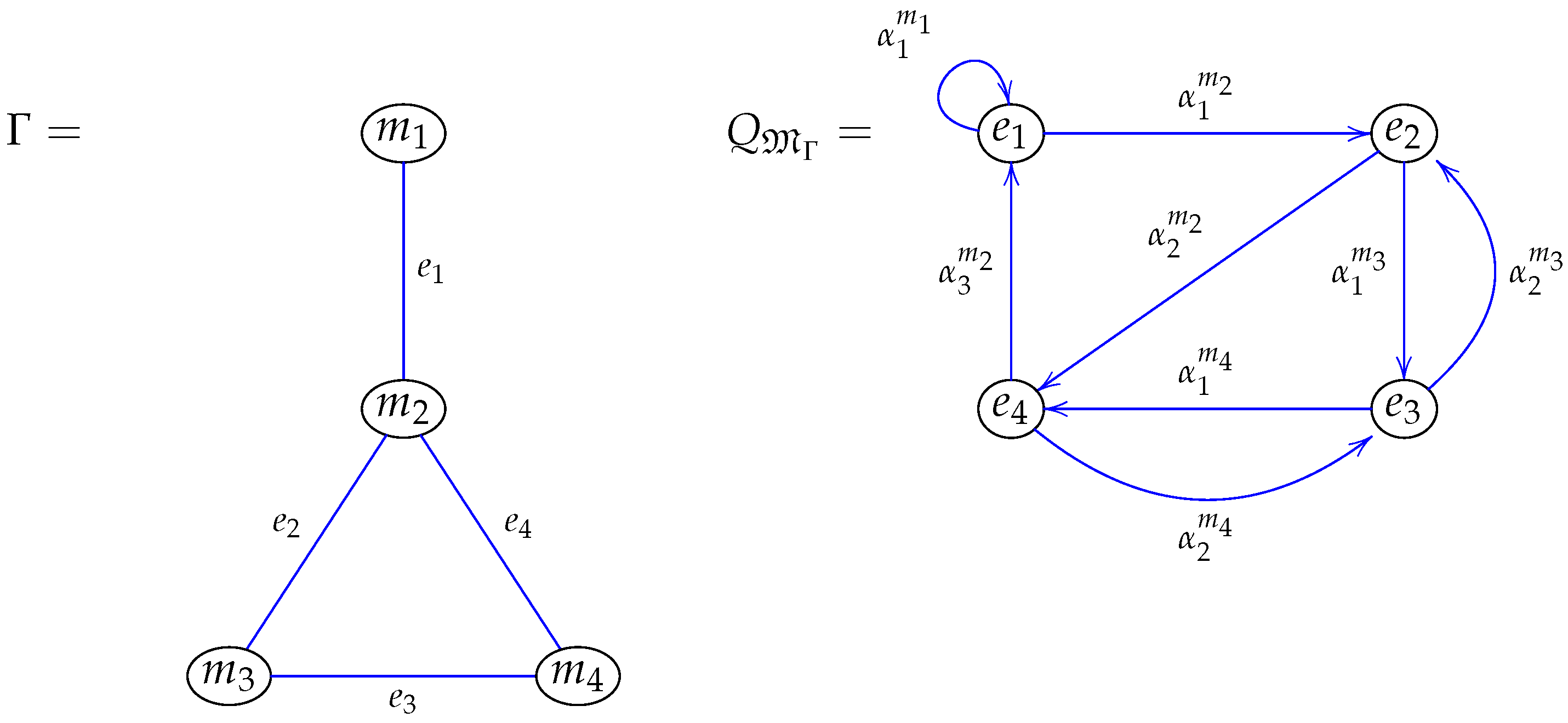
Let and be, respectively, the set of vertices and edges of a graph (see Figure 5). Then Γ defines a Brauer configuration of type M satisfying the following properties:
Figure 5.
A hair graph and its induced Brauer quiver .
- .
- .
- The degree of the vertices gives their valency values, i.e., , and , for .
- The multiplicity values of the elements of M (vertices of the Brauer configuration ) are , , , and .
- Circular orderings associated with vertices , areThese circular orderings define the orientation . The symbol in a circular ordering means that occurs q times at the polygon (edge) .
- The Brauer quiver induced by the Brauer configuration is such that the set of vertices and there exists an arrow if and only if there exists a relation in the circular ordering associated with the vertex (see Figure 5).
- The Brauer configuration algebra is the bound quiver algebra induced by the Brauer configuration , the following are examples of relations contained in the admissible ideal .
- 1.
- , , , .
- 2.
- , , , .
- 3.
- if , for all values of r and s.
- The Brauer configuration algebra is indecomposable as an algebra and reduced, provided that the Brauer quiver is connected and , for any .
- Since Γ is a hair graph of type , then the covering graph is isomorphic to Γ, whose entropies , , and (the entropy of the Brauer configuration ) are as follows:
- 1.
- .
- 2.
- .
- 3.
- , provided that . In [25], Cañadas et al. proved that if Γ is a Dynkin or Euclidean diagram, then allows for giving approximations of .
- The dimensions of the Brauer configuration algebra and its corresponding center are given by the following identities:
3. Main Results
This section gives a Brauer analysis of some generators of Thompson’s group F and provides solutions of the Yang–Baxter equation via covering graphs defined by appropriate Brauer quivers.
3.1. Brauer Analysis of Thompson’s Group F
This section introduces Brauer configuration algebras induced by a set of Thompson’s group F generators.
The following results Theorem 1 and its Corollary 1 give formulas for the center dimension of Brauer configuration algebras of type M.
Theorem 1.
The center dimension of a connected Brauer configuration algebra induced by a Brauer configuration of type M is given by the following formula (see (11)):
Proof.
It is a consequence of Formula (14); note that , which is the number of loops of induced by vertices with valency one. Furthermore, the number of loops in the Brauer quiver , induced by a vertex m contained in a polygon with , is . We are done. □
Corollary 1.
The center dimension of a connected Brauer configuration algebra induced by a Brauer configuration of type M whose polygons have no repeated elements is given by the following formula:
Proof.
We note that in this case. We are done. □
Theorem 2 defines isomorphism classes of Brauer configuration algebras induced by binary trees.
Theorem 2.
Let and be Brauer configuration algebras of type M induced by two binary trees and , where is obtained from by rotation, then and are isomorphic as algebras.
Proof.
The result follows, provided that the rotation operator preserves degree sequences. □
Let us consider now the following Brauer configurations of type M, and , where , and .
The following formulas define polygons and . For and .
Theorem 3 regards Brauer configuration algebras and , induced by Brauer configurations of type M, and .
Theorem 3.
The Brauer configuration algebras and induced by the Brauer configurations of type M, and defined by identities (21) and (22) are isomorphic as algebras.
Proof.
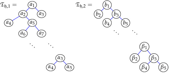
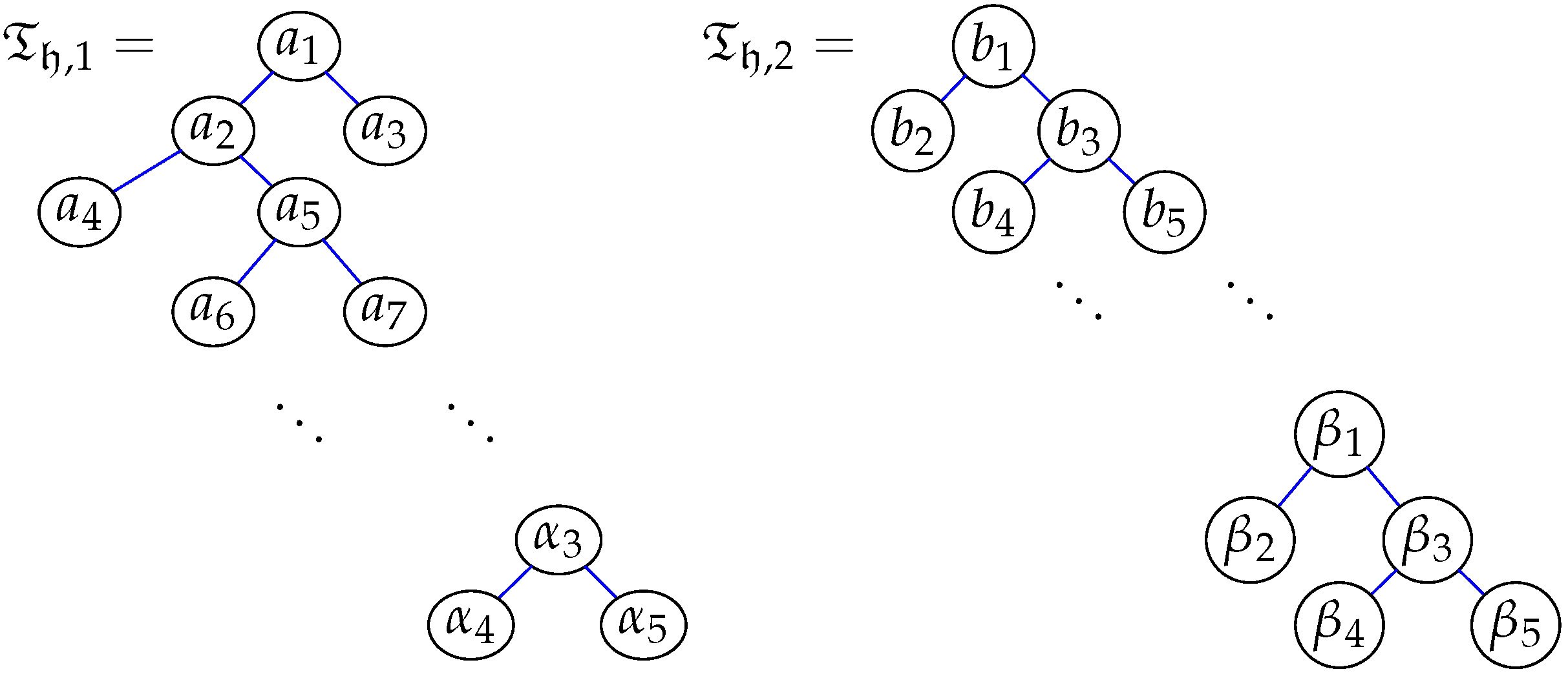
For fixed, Brauer configurations and define binary trees and shown in Figure 6 ( and ):
Figure 6.
Binary trees induced by Brauer configurations and for fixed.
Since is obtained from by rotation at the vertex , the result holds as a consequence of Theorem 2. We are done. □
Let be the decomposable Brauer configuration algebra obtained from the direct sum of the Brauer configurations and , i.e., .
According to Theorem 3, we note that each decomposable Brauer configuration of type M with , gives rise to a generator , with three breakpoints of Thompson’s group F. We let denote such a set of generators.
We note that according to Burillo [29], , so the analysis of algebraic invariants of the Brauer configurations induced by the decomposable Brauer configurations is a Brauer analysis of Thompson’s group F. In the same line, we will assume the notation for Brauer configuration algebras induced by Brauer configurations . Note that, for each generator , it holds that , where and are isomorphic Brauer configuration algebras induced by the reduced binary trees that define the generator .
Brauer configuration algebra () is said to be the first (second) projection of the Brauer configuration algebra .
Theorem 4 regards Brauer configuration algebras of type induced by generators of Thompson’s group F.
Theorem 4.
Let be the first projection of the Brauer configuration algebra of type , then the following results hold for .
- 1.
- is indecomposable as an algebra.
- 2.
- .
- 3.
- .
- 4.
- .
- 5.
- .
- 6.
- .
Proof.
- is indecomposable as an algebra provided that the binary tree , which induces , is connected.
- Note that the number of edges of the binary tree is . Furthermore, , , and . Then, .
- .
- .
- Note that, , then .
- , then . We are done.
□
Theorem 5 regards the rotation graph associated with an element of Thompson’s group F.
Theorem 5.
Let and be reduced binary trees defined by the domain and range of the product with , . Then there exists a linear path in of length connecting and .
Proof.
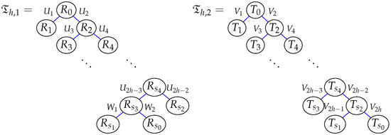
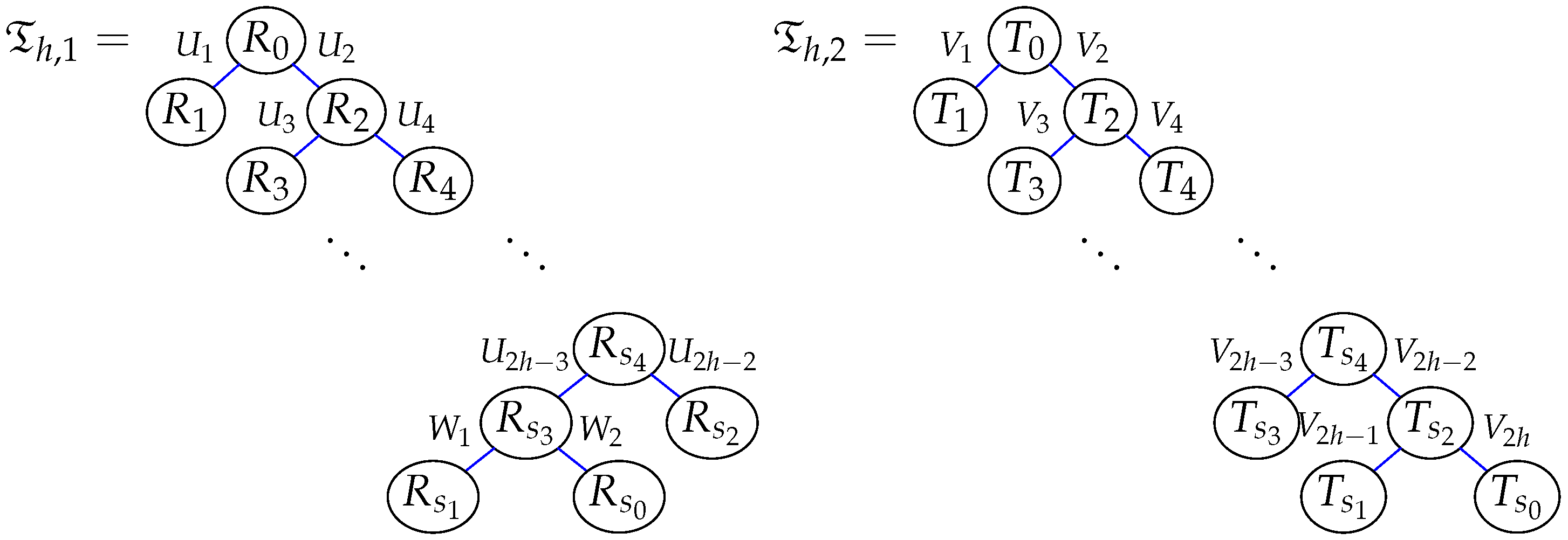
Note that the reduced binary trees and have the shapes shown in Figure 7 with , , and .
Figure 7.
Binary trees defined by the element of Thompson’s group F.
The rotation path connects binary trees and . The result holds taking into account that the size of the path P is . We are done. □
Theorem 6 is a consequence of Theorems 3, 4, and 5.
Theorem 6.
Let be the Brauer configuration algebra induced by the reduced binary tree associated with the domain of with and , then
Proof.
We note that the binary tree associated with the domain of is obtained by a tree concatenation with the following form:
At the points (vertex enumeration as shown in Figure 7). Thus, and have the same number of vertices and edges. Furthermore, they have identical degree sequences, so and can be obtained from via a finite sequence of rotations and the corresponding Brauer configuration algebras and are isomorphic. We are done. □
Theorem 7 describes covering graphs induced by Brauer configurations and defined by generators .
Theorem 7.
Let and be the Brauer quivers induced by Brauer configurations and of type and , respectively, defined by a reduced generator of Thompson’s group F, then the covering graph is isomorphic to the hair graph , whereas the covering graph is isomorphic to . Where , and are edges of binary trees and associated with the domain and range of , respectively. denotes an n-vertex linear path.
Proof.
The successor sequences and associated with nontruncated vertices have the following forms:
In this case, and . We are done. □
3.2. Solutions of the Yang–Baxter Equation Arising from Covering Graphs
For , let us define operators and , where is the set of all reduced binary trees and defined by Burillo’s generators of Thompson’s group F and
In this case, the operator deletes vertex v in a binary tree and the edge connecting it with its parent.
We let denote the product operator , such that .
Theorem 8 proves that operator allows for finding set-theoretical solutions of the Yang–Baxter equation.
Theorem 8.
Let be a generator of Thompson’s group F, then and the map is a solution of the Yang–Baxter equation (see identity (5)).
Proof.
Note that, .
To prove that is a set-theoretical solution of the Yang–Baxter equation, we study the following identity:
Indeed
- If , , , and , then=.On the other hand,.
- If , , with h, i, and f arbitraries, then=.On the other hand,.
Since the remaining cases can be verified in the same way, we conclude that the identity (26) holds. We are done. □
3.3. Brauer Analysis of Thompson’s Group F via Christoffel Words
This section defines Brauer configuration algebras induced by Christoffel words associated with some generators of Thompson’s group F.
Another approach of Brauer analysis to the theory of Thompson’s group can be realized by means of Christoffel paths and Christoffel words. According to Frosini and Tarsissi [43], in the last few decades, the theory of Christoffel words has acquired a prominent role in the study of the discretization of segments and shapes; such a theory has relationships with continued fractions, snake graphs, Markov numbers, and cluster algebras [43].
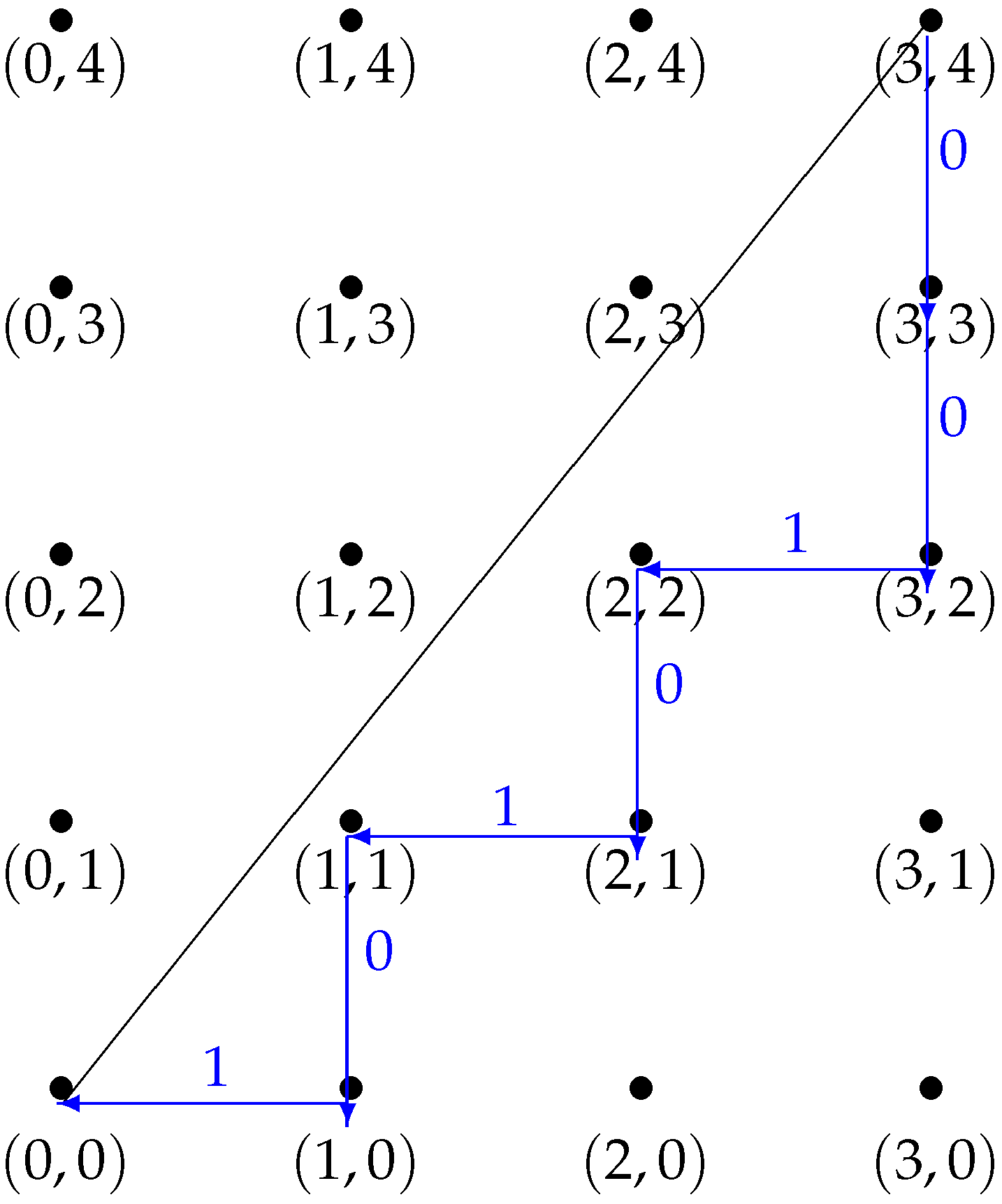
If a and b are co-prime numbers, the Christoffel path of slope is defined as the connected path in the discrete plane joining the origin to the point , such that it is the nearest path below the Euclidean line segment joining these two points, so there are no points of the discrete plane between the path and the line segment.
A Christoffel word is obtained by assigning either a 0 (1) to a vertical (horizontal) step of the Christoffel path.
The Christoffel word related to the path reaching the point is denoted as and its slope , where denotes the number of occurrences of the number x in the word w.
Figure 8 shows the lower Christoffel path associated with the line segment and the corresponding Christoffel word .

Figure 8.
Christoffel path associated with the rational number .
For , generators of Thompson’s group F give rise to Brauer configurations , of type M, where , for , the collection of polygons consists of Christoffel words defined respectively by irreducible fractions associated with generator . Note that, if , then . Furthermore, or in successor sequences, and .
We let denote the Brauer configuration algebra induced by the ordered Christoffel words of the generator .
Example 5.
In , the following identities hold:
- 1.
- , .
- 2.
- .
- 3.
- .
Theorem 9 regards Brauer configuration algebras induced by Christoffel words and the set of generators of Thompson’s group F.
Theorem 9.
For , let be the Brauer configuration algebra induced by the Brauer configuration of type M whose polygons are defined by Christoffel words of Thompson’s group generator whose breakpoints are , then the following results hold
- 1.
- is indecomposable as an algebra.
- 2.
- .
- 3.
- .
- 4.
- The covering graph is a 4-point linear path.
Proof.
- If denotes the polygon defined by the word , , then , hence the Brauer quiver induced by the Brauer configuration is connected. Therefore, the algebra is indecomposable as an algebra.
- We note that, if , and are rational numbers whose Christoffel words are , and , respectively. Then, , , , and . Therefore, , , , . Furthermore, , , , . Where, , denotes the number of occurrences of the number h in the polygon . Thus, and , then .
- Note that, for any , and , and the number of loops in the Brauer quiver induced by the Brauer configuration is . Then, .
- , where is the chain induced by the expansions of .
□
For . The sequence is said to be the Christoffel–Thompson sequence. It is encoded as the sequence A009350 in the On-Line Encyclopedia of Integer Sequences (OEIS) [44]. In such a case, if with , then .
4. Conclusions
Thompson’s group F induces decomposable Brauer configuration algebras whose Brauer analysis allows for finding formulas for their dimensions and the dimensions of their centers. We also note that it is possible to build paths by appropriately rotating the binary trees associated with Thompson’s group F generators. Such generators define Christoffel words, which induce Brauer configurations of type M. A Brauer analysis applied to these algebras allows for giving their dimensions and the structure of corresponding covering graphs.
The covering graph induced by Thompson’s group F generators allows for the formulation of set-theoretical solutions of the Yang–Baxter equation.
Our comments on future work are as follows:
- Applying Brauer analysis to generators of Thompson’s group T and V is an open problem. Such an analysis can include giving values of the super edge-magic total strength of covering graphs, as Deepthi defined in [45].
- Another task for the future consists of giving new solutions of the Yang–Baxter equation arising from the Brauer configuration algebras induced by generators of Thompson’s group T and V.
- Applying Brauer analysis to quantum circuits is a task to be addressed in the future, assuming quantum gates as elements of the ground set M and quantum circuits as elements of a collection of multisets denoted in this paper.
Author Contributions
Investigation, writing, review, and editing, A.M.C., J.G.R.-N., O.P.S.-D., R.V., and H.G. All authors have read and agreed to the published version of the manuscript.
Funding
Convocatoria Nacional para el Establecimiento de Redes de Cooperación bajo el Marco del Modelo Intersedes 2022–2024, Universidad Nacional de Colombia. Cod Hermes 59773.
Data Availability Statement
The original contributions presented in this study are included in the article. Further inquiries can be directed to the corresponding author.
Conflicts of Interest
The authors declare no conflicts of interest.
Abbreviations
The following abbreviations are used in this manuscript:
| Binary tree defined by Thompson’s group generator | |
| Christoffel path | |
| Covering graph of a Brauer quiver | |
| Dimension of a Brauer configuration algebra | |
| Dimension of the center of a Brauer configuration algebra | |
| Entropy of a graph | |
| Entropy of a Brauer configuration induced by a graph | |
| Hair graph | |
| Brauer configuration algebra | |
| Rotation graph whose set of vertices are n-vertex binary trees | |
| M | Set of vertices of a Brauer configuration |
| Collection of polygons of a Brauer configuration | |
| Brauer configuration | |
| Multiplicity function of a Brauer configuration | |
| Orientation of a Brauer configuration | |
| valency of a vertex x | |
| YBE | Yang–Baxter equation |
| Center of a Brauer configuration algebra |
References
- Brin, M.; Squier, C. Groups of piecewise linear homeomorphisms of the real line. Inventiones. Math. 1985, 79, 485–498. [Google Scholar] [CrossRef]
- Higman, G. Finitely Presented Infinite Simple Groups; Notes on Pure Mathematics; Dept. of Pure Mathematics, Dept. of Mathematics, I.A.S., Australian National University: Canberra, Australia, 1974; Volume 8, Available online: https://api.semanticscholar.org/CorpusID:116374349 (accessed on 12 August 2024).
- Brown, K.S. Finiteness properties of groups. J. Pure Appl. Algebra 1987, 44, 45–75. [Google Scholar] [CrossRef]
- McKenzie, R.; Thompson, R.J. An Elementary Construction of Unsolvable Word Problems in Group Theory; Boone, W.W., Cannonito, F.B., Lyndon, R.C., Eds.; Word Problems: North-Holland, The Netherlands, 1973; pp. 35–55. Available online: https://api.semanticscholar.org/CorpusID:118246987 (accessed on 15 August 2024).
- Freyd, P.; Heller, A. Splitting homotopy idempotents. J. Pure Appl. Algebra 1993, 89, 93–106. [Google Scholar] [CrossRef]
- Ohshika, K.; Papadopoulos, A.; Penner, R.C.; Wienhard, A. New trends in Teichmüller theory and mapping class groups. Oberwolfach Rep. 2018, 15, 2475–2534. [Google Scholar] [CrossRef]
- Sleator, D.D.; Tarjan, R.E. A data structure for dynamic trees. J. Comput. Syst. Sci. 1983, 26, 362–391. [Google Scholar] [CrossRef]
- Sleator, D.D.; Tarjan, R.E.; Thurston, W.P. Rotation distance, triangulations, and hyperbolic geometry. J. Am. Math. Soc. 1988, 1, 122–135. [Google Scholar] [CrossRef]
- Cañadas, A.M.; Bravo, G. Dyck path categories and its relationships with cluster algebras. J. Algebra Its Appl. 2022, 23, 2430001. [Google Scholar] [CrossRef]
- Green, E.L.; Schroll, S. Brauer configuration algebras: A generalization of Brauer graph algebras. Bull. Sci. Math. 2017, 121, 539–572. [Google Scholar] [CrossRef]
- Cañadas, A.M.; Gutierrez, I.; Mendez, O.M. Brauer Analysis of Some Cayley and Nilpotent Graphs and Its Application in Quantum Entanglement Theory. Symmetry 2024, 16, 570. [Google Scholar] [CrossRef]
- Cañadas, A.M.; Angarita, M.A.O. Brauer configuration algebras for multimedia based cryptography and security applications. Multimed. Tools. Appl. 2021, 80, 23485–23510. [Google Scholar] [CrossRef]
- Yang, C.N. Some exact results for the many-body problem in one dimension with repulsive delta-function interaction. Phys. Rev. Lett. 1967, 19, 1312–1315. [Google Scholar] [CrossRef]
- Lieb, E.H.; Liniger, W. Exact analysis of an interacting Bose gas. I. The general solution and the ground state. Phys. Rev. 1963, 130, 1605–1616. [Google Scholar] [CrossRef]
- Baxter, R.J. Partition function for the eight-vertex lattice model. Ann. Phys. 1972, 70, 193–228. [Google Scholar] [CrossRef]
- Lieb, E.H. Exact analysis of an interacting Bose gas. II. The excitation spectrum. Phys. Rev. 1963, 130, 1616–1624. [Google Scholar] [CrossRef]
- Caudrelier, V.; Crampé, N. Exact results for the one-dimensional many-body problem with contact interaction: Including a tunable impurity. Rev. Math. Phys. 2007, 19, 349–370. [Google Scholar] [CrossRef]
- Aharonov, D.; Jones, V.; Landau, Z. A Polynomial Quantum Algorithm for Approximating the Jones Polynomial. Algorithmica 2009, 55, 395–421. [Google Scholar] [CrossRef]
- Pachos, J.K. The Jones polynomial algorithm. In Introduction to Topological Quantum Computation; Cambridge University Press: Cambridge, UK, 2012; pp. 157–176. [Google Scholar] [CrossRef]
- Dehornoy, P. The group of parenthesized braids. Adv. Math. 2006, 205, 354–409. Available online: https://www.sciencedirect.com/science/article/pii/S0001870805002045 (accessed on 25 July 2024). [CrossRef]
- Jones, F.R.V. Some unitary representations of Thompson’s groups F and T. J. Comb. Algebra 2017, 1, 1–44. [Google Scholar] [CrossRef]
- Cañadas, A.M.; Ballester-Bolinches, A.; Gaviria, I.D.M. Solutions of the Yang-Baxter equation arising from Brauer configuration algebras. Computation 2022, 11, 2. [Google Scholar] [CrossRef]
- Rump, W. Modules over braces. Algebra Discret. Math. 2006, 2, 127–137. Available online: https://admjournal.luguniv.edu.ua/index.php/adm/article/view/892 (accessed on 15 July 2024).
- Cedó, F.; Jespers, E.; Oniński, J. Braces and the Yang-Baxter equation. Commun. Math. Phys. 2014, 327, 101–116. [Google Scholar] [CrossRef]
- Cañadas, A.M.; Espinosa, P.F.F.; Nieto, J.G.R.; Mendez, O.M.; Arteaga-Bastidas, R.H. Extended Brauer Analysis of Some Dynkin and Euclidean Diagrams. ERA 2024, 32, 5752–5782. [Google Scholar] [CrossRef]
- Schroll, S. Brauer Graph Algebras. In Homological Methods, Representation Theory, and Cluster Algebras; Assem, I., Trepode, S., Eds.; CRM Short Courses; Springer: Cham, Switzerland, 2018; pp. 177–223. [Google Scholar] [CrossRef]
- Espinosa, P.F.F. Categorification of Some Integer Sequences and Its Applications. Ph.D. Thesis, National University of Colombia, Bogotá, Colombia, 2021. Available online: https://repositorio.unal.edu.co/handle/unal/79501 (accessed on 1 July 2024).
- Belk, J.M. Thompson’s Group F. Ph.D. Thesis, Cornell University, Ithaca, NY, USA, 2004. Available online: https://pi.math.cornell.edu/~belk/Thesis.pdf (accessed on 1 July 2024).
- Burillo, J. Introduction to Thompson’s Group F. UPC Universitat Politècnica de Catalunya. Available online: https://api.semanticscholar.org/CorpusID:250274227 (accessed on 5 July 2024).
- Cannon, J.W.; Floyd, W.J.; Parry, W.R. Introductory notes on Richard Thompson’s groups. L’Enseignement Mathématique 1996, 42, 215–256. Available online: https://www.imo.universite-paris-saclay.fr/~emmanuel.breuillard/Cannon.pdf (accessed on 18 August 2024).
- Nichita, F.F. Introduction to the Yang-Baxter equation with open problems. Axioms 2012, 1, 33–37. [Google Scholar] [CrossRef]
- Drinfeld, V.G. On Unsolved Problems in Quantum Group Theory; Lecture Notes Math.; Springer: Berlin, Germany, 1992; Volume 1510, pp. 1–8. [Google Scholar] [CrossRef]
- Ballester-Bolinches, A.; Esteban-Romero, R.; Fuster-Corral, N.; Meng, H. The structure group and the permutation group of a set-theoretical solution of the quantum Yang-Baxter equation. Mediterr. J. Math. 2021, 18, 1347–1364. [Google Scholar] [CrossRef]
- Etingof, P.; Soloviev, A.; Guralnick, R. Indecomposable set-theoretical solutions to the quantum Yang-Baxter equation on a set with a prime number of elements. J. Algebra 2001, 242, 709–719. [Google Scholar] [CrossRef]
- Nichita, F.F. Yang-Baxter equations, computational methods and applications. Axioms 2015, 4, 423–435. [Google Scholar] [CrossRef]
- Etingof, P.; Schedler, T.; Soloviev, A. Set-theoretical solutions to the quantum Yang-Baxter equation. Duke Math. J. 1999, 100, 169–209. [Google Scholar] [CrossRef]
- Gateva-Ivanova, T.; Van den Bergh, M. Semigroups of I-type. J. Algebra 1998, 206, 97–112. [Google Scholar] [CrossRef]
- Guarnieri, L.; Vendramin, L. Skew braces and the Yang-Baxter equation. Math. Comput. 2017, 85, 2519–2534. Available online: https://www.jstor.org/stable/90010152 (accessed on 3 March 2024). [CrossRef]
- Andrews, G.E. The Theory of Partitions; Cambridge University Press: Cambridge, UK, 2010. [Google Scholar] [CrossRef]
- Sierra, A. The dimension of the center of a Brauer configuration algebra. J. Algebra 2018, 510, 289–318. [Google Scholar] [CrossRef]
- Rashevsky, N. Life, information theory, and topology. Bull. Math. Biophys. 1955, 17, 229–235. [Google Scholar] [CrossRef]
- Trucco, E. A note on the information content of graphs. Bull. Math. Biol. 1956, 18, 129–135. [Google Scholar] [CrossRef]
- Frosini, A.; Tarsissi, L. The characterization of the minimal paths in the Christoffel tree according to a second-order balancedness. Developments in Language Theory-DLT2020; Tampa, USA. 2020, pp. 1–14. Available online: https://hal.science/hal-02495529v1 (accessed on 20 August 2024).
- Sloane, N.J.A. The On-Line Encyclopedia of Integer Sequences. Available online: https://oeis.org/A009350 (accessed on 19 August 2024).
- Deepthi, N.S. Super Edge-magic Total Strength of Some Unicyclic Graphs. Ars Comb. 2024, 159, 73–85. [Google Scholar] [CrossRef]


Disclaimer/Publisher’s Note: The statements, opinions and data contained in all publications are solely those of the individual author(s) and contributor(s) and not of MDPI and/or the editor(s). MDPI and/or the editor(s) disclaim responsibility for any injury to people or property resulting from any ideas, methods, instructions or products referred to in the content. |
© 2025 by the authors. Licensee MDPI, Basel, Switzerland. This article is an open access article distributed under the terms and conditions of the Creative Commons Attribution (CC BY) license (https://creativecommons.org/licenses/by/4.0/).