Splitting and Merging for Active Contours: Plug-and-Play

Abstract

This study tackles the challenge of splitting and merging in parametric active contours or snakes. The proposed method comprises three stages: (1) fully 4-connected interpolation, (2) snake splitting, and (3) snakes merging. For this purpose, first, the coordinates of snake points are separated into two corrupted 1D signals, with missing X/Y samples in the signals representing missing snakes’ coordinates. These missing X/Y samples are estimated using a constrained Tikhonov regularisation model, ensuring fully 4-connected snakes. Next, crossing points are identified by plotting snake points onto a raster matrix, detecting overlaps where multiple snake points occupy the same raster cell. Finally, snakes are split or merged by extracting snake points between crossing snake points that form a loop using a heuristic approach. Experimental results on the boundary detection of enamel in Micro-CT images and coronary arteries’ lumen in CT images demonstrate the proposed method’s ability to handle contour splitting and merging effectively.

1. Introduction

1.1. Background

Image segmentation is the process of partitioning an image into meaningful regions. Active contour (AC) models, or snakes, play a crucial role in segmentation by evolving a curve towards object boundaries through energy minimisation techniques. These models incorporate edge information, region statistics, and shape priors to enhance segmentation accuracy, making them particularly effective for detecting complex and irregular structures [1]. The AC model, initially proposed by Kass et al. [2], is a framework where a curve dynamically evolves to minimise defined energy functions. Parametric ACs, or “snakes”, are represented as a parameterised $\mathit{c}\left(s\right)=\left(x\left(s\right),y\left(s\right)\right)$, where $s\in \left[\mathrm{0,1}\right]$ is a parameter. The evolution of the curve is governed by minimising $E_{snake}=E_{internal}+E_{image}+E_{external}$ where $E_{internal}$ ensures smoothness of the curve, defined as: $E_{internal}={\int }_0^1\left(\alpha {‖{\mathit{c}}^{\prime }\left(s\right)‖}^2+\beta {‖{\mathit{c}}^{″}\left(s\right)‖}^2\right)ds$, where ${\mathit{c}}^{\prime }\left(s\right)$ and ${\mathit{c}}^{″}\left(s\right)$ are the first- and second-order derivatives, and $\alpha$ and $\beta$ are weighting parameters. $E_{image}$ attracts the curve toward image features such as edges: $E_{image}=-{\int }_0^1{\left|\nabla I\left(\mathit{c}\left(s\right)\right)\right|}^{2}ds$, where $I(x,y)$ is the image intensity and $\nabla I$ is its gradient. Finally, $E_{external}$ incorporates other forces (e.g., user-defined constraints). Since its introduction, numerous advancements have been made to enhance the snake’s efficiency to address more complex and challenging image segmentation tasks. In recent years, Deep Snake [3] has reignited interest in snake models, a topic that had long been overlooked after the development of data-driven image segmentation methods. Deep learning techniques have contributed to this resurgence by enhancing the flexibility and accuracy of traditional snakes in image segmentation and object boundary detection. However, the key limitations of snakes including the splitting of a parametric contour into multiple contours or the merging of multiple parametric contours into a unique contour have not been addressed in their entirety [4].

• Merging: When two distinct contours (e.g., two objects) approach and eventually collide, the AC model must be capable of merging them into a single contour.
• Splitting:

  ■

  Object Splitting: An object can split into multiple contours (e.g., during cell mitosis). The AC should effectively handle this process, ensuring a clear separation into distinct contours.

  ■

  Self-loop: During evolution, the AC may form small loops within itself, which are undesirable artefacts. These loops typically arise due to the improper handling of contour evolution or issues in the energy minimisation process.

Research addressing these limitations has generally followed two main directions: geometric ACs (GACs) and non-GACs. The following subsection reviews previous methods proposed for splitting and merging of snake models based on these directions.

1.2. Reviewing Splitting and Merging Methods

1.2.1. GACs

GACs are a class of AC models that, unlike snakes, explicitly represent the contour as a deformable curve using an implicit representation based on level set methods. This approach enables the contour to handle topology changes without requiring additional modifications. GACs are widely used in medical imaging, object tracking, and computer vision due to their flexibility in capturing complex shapes. GACs were independently introduced by Caselles et al. [4] and Malladi et al. [5], building upon curve evolution theory [6] and the level set method, where the curve $\mathit{c}=\left\{\left(x,y\right):\varphi \left(x,y\right)=0\right\}$ is implicitly represented as the zero level set of a higher-dimensional function $\varphi \left(x,y\right)$ [7]. The evolution of $\varphi$ is governed by the Hamilton–Jacobi equation: ${\displaystyle \frac{\partial \varphi }{\partial t}}=‖\nabla \varphi ‖\left(\kappa +F_{image}\right)$, where $\nabla \varphi$ is the gradient norm, ensuring proper propagation. $\kappa$ is the curvature of the contour, defined as: $\kappa =\nabla ·\left({\displaystyle \frac{\nabla \varphi }{‖\nabla \varphi ‖}}\right)$, which promotes smoothness. $F_{image}$ is an image-based term, such as: $-\left|\nabla I \right|$, attracting the curve to edges. GACs are further classified into edge-based and region-based methods. In edge-based GACs, the evolving contour is represented as the zero level set of a higher-dimensional embedding function. The contour evolves in the direction perpendicular to the image gradient, stopping at the desired boundary. While edge-based GACs handle topological changes automatically and allow the incorporation of arbitrary geometric or topological constraints, they face significant challenges in introducing user-defined external forces [8]. Furthermore, edge-based GACs are highly sensitive to image noise, weak gradients, or discontinuities in boundaries [9]. To address the limitations of edge-based GACs, region-based GACs were proposed by Chan and Vese [10], Samson et al. [11], and Yezzi et al. [12]. Region-based methods incorporate image region information rather than relying solely on gradient features, improving robustness in challenging scenarios. However, these models are often restricted to a finite number of image regions, limiting their flexibility.

Despite their strengths, the primary drawback of all GAC methods is their computational complexity, leading to high execution times. This limitation hinders their application in real-time tasks, such as online target tracking, where rapid contour evolution is essential.

1.2.2. Non-GACs

Unlike GACs, non-GAC methods are mostly based on computational geometry and focus on the shape and properties of the contour. These methods leverage geometric principles to address curve intersections or topological changes and can be categorised into several distinct classes.

Grid-Based

The first category is the grid-based approach, introduced by McInerney and Terzopoulos as “T-snakes” [8]. This method integrates the AC with a graphical decomposition approach. It employs a simplicial affine cell image decomposition method, also known as triangulation, to iteratively reparameterise snakes in two phases. This technique enables topology transformations and handles collisions effectively. While the T-Snake achieves topological adaptability, it compromises accuracy due to the use of simplicial approximations. Delingette and Montagnat [13] extended the grid-based concept by employing a regular grid not for reparameterisation but to detect intersecting edges. Through their method, the candidates for intersecting edges were stored in a hash table, and topology modification was achieved based on distances between the snakes. Bischoff and Kobbelt [14,15] introduced restricted snake method to reduce computational complexity by dividing images into uniform square grids and confining the positions and movements of snake points to the grid lines. However, this reduction in computation time comes at the cost of accuracy. Additionally, the restricted snake method struggles to perform well in regions with deep concavities and small tubular branches. Oliveira et al. [16,17] introduced the concept of loop snakes to control the self-crossing of T-snakes. In their approach, self-crossing was approximated by piecewise linear mapping. Then, with the aid of additional structural analysis, termed the loop-tree, they determined whether the enclosed region was explored by the snake. Finally, Zheng [18] proposed an enhancement to the original T-snakes by introducing stricter constraints. These constraints limit the movement of snake points to orthogonal equidistant paths, ensuring that each point moves exclusively from one vertex to another.

Force-Based

The second class encompasses approaches that either contribute to or utilise AC forces to handle topological changes. Ivins and Porrill [19] proposed the application of a repulsion force, calculated based on stiffness, tension, and reversed pressure, to prevent self-crossing in snakes. Ďurikovič et al. [20] introduced an area-based force, defined as a discrete approximation of the inner normal vector to the snake. This area-based force initially prevents formation of self-crossings. Wong et al. [21] developed an AC approach for detecting bottleneck edges while avoiding self-collision of AC. Their method involves disconnecting the closed snake into multiple open snakes and guiding the snakes toward bottleneck edges using a force. A scaling function was used to adjust the normal forces acting on the open snakes, while preventing the formation of self-crossing loops. Choi et al. [22] leveraged image forces near the snake points to identify critical points prone to splitting. Then, splitting was executed between point pairs separated by distances below a specified threshold. Lefèvre and Vincent [23] used external energy information to detect splitting points on the snake. Specifically, snake points trapped in the background, where the external energy fell below a noise robust threshold, were identified as splitting points. New snakes were subsequently created from successive points. Li et al. [24] utilised the Gradient vector flow (GVF) as an external force to enable snake splitting in multi-object segmentation tasks. Their approach first segmented all objects into a single region using the external force field. Subsequently, snake splitting was performed along the boundaries of the segmented regions. Similar strategies to those employed by Li et al. [24] can be found in related works [25,26].

Computational Geometry-Based

The third category encompasses intersection detection methods, including brute force, sweep line [27], and sweep-and-prune [28], which are well-established in the field of computational geometry. The brute force algorithm systematically examines all pairs of line segments, formed by connecting successive snake points, to identify intersections. In contrast, the sweep line algorithm introduces a dynamic approach, where a line sweeps across the image plane, recording events as it intersects line segments. At each position of the sweep line, information about segments it intersects is stored in a data structure. This data structure, which is an ordered list of intersected segments, facilitates intersection detection and is dynamically updated as the sweep progresses. Finally, the sweep-and-prune algorithm enhances the sweep line technique by optimising the sorting process, only reordering relevant portions of the list rather than the entire structure. Examples of applying these techniques on handling AC topological changes can be found in [29,30,31,32].

Distance-Based

The fourth category represents a straightforward approach based on measuring the distances between snake points to identify intersections [33]. Araki et al. [34] proposed a method for detecting crossing points between two line segments $v_i{v}_{i+1}$ and $v_j{v}_{j+1}$ ($v$ is a snake point and $j\ne i-1,i,i+1$). They identified an intersection if the equation $p\left(v_{i+1}-v_i\right)=q(v_{j+1}-v_j)$ yielded roots $p,q$ where $0<p<1$ and $0<q<1$. This model was later extended for merging multiple snakes [35]. Ngoi and Jia [36] introduced a positive-negative contour approach to prevent self-loop formation and facilitate contour splitting during multiple object segmentation by measuring the distance between snake points. Similarly, Nakaguro and Makhanov [37] used a distance threshold to detect intersections and proposed a model that allowed multiple snakes to split and merge while employing quadratic constraints [38] to avoid self-looping. Lefèvre and Vincent [23] merged snakes by comparing the centres of gravity, calculated as the mean of the X and Y coordinates of all snake points. If the distance between two centres was below a set threshold, the snakes were merged. Mikula et al. [39,40] introduced a grid-based method to efficiently detect self-crossing by identifying grid boxes containing multiple non-consecutive snake points. This approach was generalised by Benninghoff and Garcke for complex topological scenarios [41] and extended to accommodate free-endpoint snakes [42].

Snake Interpolation-Based

The final approach focuses on fully connecting snake points to identify intersection points. Challenges with this approach are false positive and false negative intersection points (illustrated in Figure 1) introduced during the discretisation of snake points (dashed line in Figure 1). Ji and Yan [43] proposed a linear interpolation method to detect intersection points, effectively making snake points continuously connected on a discrete plane. To mitigate the false positive issue, they employed a distance threshold to filter out erroneous detections. Their method was later extended to address the problem of merging snakes [44]. Building on this work, Nakhmani and Tannenbaum [45] introduced a 4-connected linear interpolation technique that effectively resolved the issue of false negatives.

Figure 1. False positive (detecting an intersection when no crossing has occurred) and false negative (not detecting an intersection when an actual crossing has occurred).

In addition to the above categories, AC models can be classified based on their ability to handle various topological changes, such as merging and splitting. The splitting problem can be further divided into two sub-problems: (1) the segmentation of multiple objects within an initial contour, where the primary snake is divided into multiple snakes, and (2) resolving the small self-loops that form when the internal resistance of snake points becomes highly uneven, leading to the creation of self-loops [44]. Two main strategies are employed to manage self-looping: the first strategy aims to prevent self-loop formation, while the second focuses on eliminating self-loops after their formation. Table 1 summarises the reviewed methods in this section.

Table 1. A review of the methods that address topological issues in AC models.

Categories	Sub-Categories	Methods	Topological Handling				Drawbacks
			Merging	Splitting
				Multiple Object	Self-Crossing
					Pre-Formation	Post-Formation
ACs	Grid-based	McInerney and Terzopoulos [8], Oliveira et al. [16,17]	√	√		√	- Not detecting all intersections due to discretisation [44]. - Deal only with rigid deformation of snakes [44].
		Bischoff and Kobbelt [14,15]		√	√
		Zheng [18]		√		√
		Delingette and Montagnat [13]	√	√		√	- Intersection detection is restricted by the size of grid [13].
	Force-based	Ivins and Porrill [19], Wong et al. [21]			√		- Not always successful prevention of self-loop [45]. - Restricting snakes’ dynamic and convergence [45].
		Ďurikovič et al. [20], Choi et al. [22]		√	√		- Unable to deal with complex objects due to limiting speed of snake’s points to equal value [13].
		Lefèvre and Vincent [23]		√			- False positive in detecting intersection points. - Limiting external energy.
		Li et al. [24], Xingfei and Jie [25], Chuang and Lie [26]		√			- Time consuming due to prior need to GVF field before snake deformation [26].
	Computational geometry-based	Smith and Schaub [29], Perrin et al. [30], Doğan et al. [31], Stoeter and Papanikolopoulos [32]	√	√		√	- Difficult implementation due to existence of different special cases [45].
	Distance-based	Pauš and Beneš [33]	√	√		√	- False positive or negative in detecting intersection points.
		Araki et al. [34]		√		√
		Araki et al. [35]	√	√		√
		Ngoi and Jia [36]		√	√
		Nakaguro and Makhanov [37]	√	√	√
		Lefèvre and Vincent [23]	√
		Mikula et al. [39,40]		√		√	- False positive or negative in detecting intersection points. - Intersection detection is restricted by the size of the grid.
		Benninghoff and Garcke [41,42]	√	√		√
	Snake interpolation-based	Ji and Yan [43]		√		√	- False negative and positive.
		Ji and Yan [44]	√	√		√	- Linear interpolation. - False negative and positive.
		Nakhmani and Tannenbaum [45]		√		√	- False positive.
GACs	Edge-based	Caselles et al. [4], Malladi et al. [5]	√	√	√		- Difficulties in admitting imposition of arbitrary geometric or topological constraints [8] and adding user-defined external force. - Susceptible to noise, low gradient or boundary gap [9]. - High execution time [24].
	Region-based	Chan and Vese [10], Samson et al. [11], Yezzi et al. [12]	√	√	√		- Supervised usage or pre-specified number of regions [24]. - High execution time [24].

1.3. Motivation and Innovation

In this paper, building on the work of Nakhmani and Tannenbaum [45], we extend the approach to address both the merging of collided snakes and the splitting of a contour. Our contributions are two-fold: (1) we propose a novel nonlinear fully 4-connected interpolation method, which overcomes the limitations of linear interpolation in merging scenarios, as illustrated in Figure 2 where linear interpolation cannot detect intersection; and (2) we develop an advanced merging algorithm capable of extracting all snakes, including both the main external and internal snakes, following a collision.

Figure 2. Inefficiency of linear 4-connected interpolation for detecting intersection points. (a) Collided snakes, (b) result of linear 4-connected interpolation, and (c) result of nonlinear 4-connected interpolation.

2. Materials and Methods

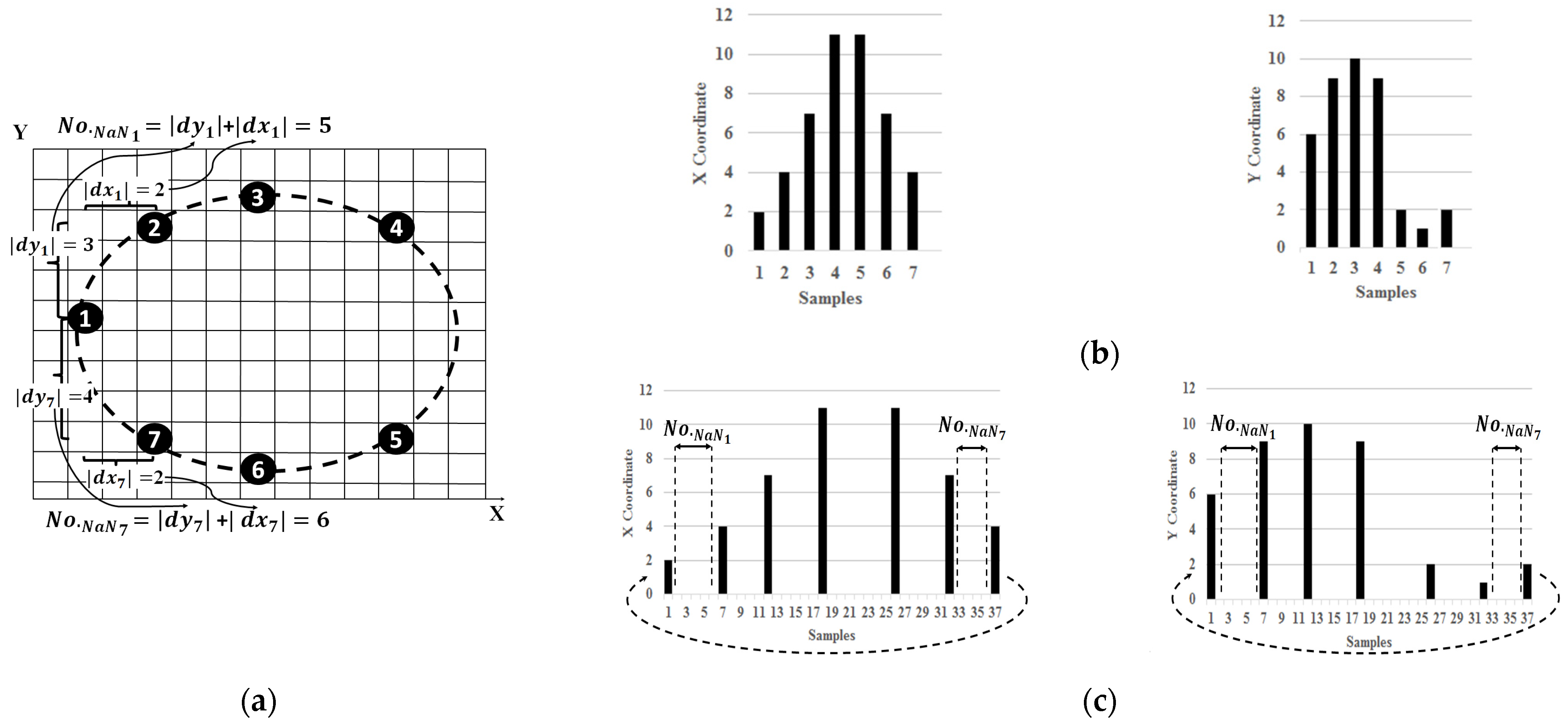
2.1. Fully 4-Connected Interpolation

To form a fully 4-connected snake on a discrete image plane, the difference in coordinates between any two successive snake points must meet specific criteria: along one axis (X or Y) the difference must be exactly one, while along the other axis it must be zero (Figure 3).

Figure 3. Relationship between coordinates of two successive pixels in a 4-connected neighbourhood.

To achieve this, we leverage a well-established 1D signal processing method known as error concealment. In this approach, unknown or missing samples are estimated based on the available known samples. Figure 4 illustrates the application of an error concealment technique, where missing data points are reconstructed using a least-squares optimisation method. In the subsequent subsections, we first reformulate the task of achieving fully 4-connected interpolation of snake points as an error concealment problem. We then propose a constrained Tikhonov regularisation model to solve the error concealment problem effectively. Finally, we extract the location information of the connector points from the solution and embed it back into the image plane.

Figure 4. (a) Corrupted signal; (b) Retrieved signal after using least square error concealment method.

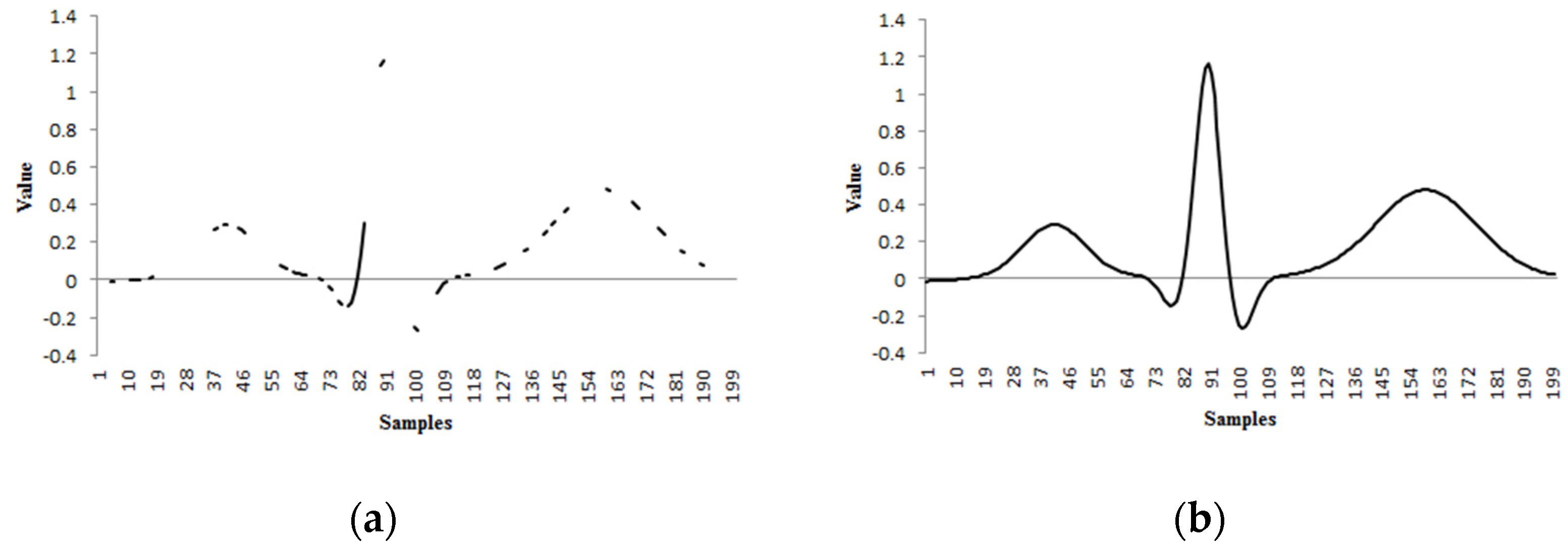
2.1.1. Transformation of 4-Connected Interpolation Problem to Error Concealment

Since the X- and Y-coordinates of snake point locations are independent, the estimation of the X- and Y-coordinates of the connector points can be performed separately. By separating the X- and Y-coordinates of the snake points into two signal vectors, ${\left({\mathit{c}}_x\left(n\right),{\mathit{c}}_y\left(n\right)\right)}_{n=1}^N$, as known samples (Figure 5b), and inserting missing samples represented by $NaN$ (Not a Number) values between the known samples (Figure 5c), the problem is reformulated as an error concealment problem. As shown in Figure 5a, the number of missing samples between each pair of known samples is calculated as ${No.}_{NaN}=(\left|d\mathit{x}\right|+\left|d\mathit{y}\right|)$.

Figure 5. Transformation of fully 4-connected snake point interpolation to an error concealment problem. (a) An example of a snake with 7 points; (b) segregating X- and Y-coordinates of snakes’ points into two signals (${\mathit{c}}_x$and ${\mathit{c}}_y$) as known samples; and (c) formation of corrupted signal by adding missing samples.

2.1.2. Mathematical Notations

Before mathematically formulating the proposed error concealment model, we first introduce some key notations. Let $\mathit{y}$ represent a corrupted signal of length $N$, and let $K$ denote the number of known samples in $\mathit{y}$, where $K<N$. Define $\mathit{S}$ as a sampling matrix of size $K\times N$. For example, if the first, third, and sixth samples of a 6-point signal $\mathit{y}$ are $\mathit{y}\left(1\right),\mathit{y}\left(3\right)$, and $\mathit{y}\left(6\right)$, then the sampling matrix $\mathit{S}$ is given by:

$$\mathit{S}=\left[\begin{array}{cc}\begin{array}{ccc}1& 0& 0\\ 0& 0& 1\\ 0& 0& 0\end{array}& \begin{array}{ccc}0& 0& 0\\ 0& 0& 0\\ 0& 0& 1\end{array}\end{array}\right].$$

(1)

The sampling matrix $\mathit{S}$ is essentially an identity matrix with the rows corresponding to missing samples removed. For instance, applying $\mathit{S}$ to the signal $\mathit{y}$, i.e., $\mathit{S}\mathit{y},$ removes the three corrupted samples, leaving only the known samples.

$$\mathit{S}\mathit{y}=\left[\begin{array}{cc}\begin{array}{ccc}1& 0& 0\\ 0& 0& 1\\ 0& 0& 0\end{array}& \begin{array}{ccc}0& 0& 0\\ 0& 0& 0\\ 0& 0& 1\end{array}\end{array}\right]\left[\begin{array}{c}\begin{array}{c}\mathit{y}\left(0\right)\\ \mathit{y}\left(1\right)\end{array}\\ \begin{array}{c}\mathit{y}\left(2\right)\\ \mathit{y}\left(3\right)\end{array}\\ \begin{array}{c}\mathit{y}\left(4\right)\\ \mathit{y}\left(5\right)\end{array}\end{array}\right]=\left[\begin{array}{c}\mathit{y}\left(0\right)\\ \mathit{y}\left(2\right)\\ \mathit{y}\left(5\right)\end{array}\right].$$

(2)

Also, we define ${\mathit{D}}^{\prime }$ and ${\mathit{D}}^{″}$ as first- and second-derivative matrices, respectively, as follows:

$${\mathit{D}}^{\prime }=\left[\begin{array}{ccc}\begin{array}{ccc}1& -1& 0\\ 0& 1& -1\end{array}& \cdots & 0\\ ⋮& \ddots & ⋮\\ 0& \cdots & \begin{array}{cc}1& -1\end{array}\end{array}\right],$$

(3)

$${\mathit{D}}^{″}=\left[\begin{array}{ccc}\begin{array}{ccc}1& -2& \begin{array}{ccc}1& 0& 0\end{array}\\ 0& 1& \begin{array}{ccc}-2& 1& 0\end{array}\\ 0& 0& \begin{array}{ccc} 1& -2& 1\end{array}\end{array}& \cdots & 0\\ ⋮& \ddots & ⋮\\ 0& \cdots & \begin{array}{ccc}1& -2& 1\end{array}\end{array}\right].$$

(4)

2.1.3. Constrained Tikhonov Regularisation Model

Tikhonov Regularisation is a technique used to stabilise ill-posed problems, by introducing a regularisation term that penalises large or unrealistic solutions. In the context of error concealment—such as video streaming or image processing—this method can be employed to recover missing or corrupted data, ensuring visually or perceptually smooth results. Mathematically, Tikhonov regularisation involves minimising the objective function [46]:

$$\begin{array}{cc}\mathit{m}\mathit{i}\mathit{n}& {‖\mathit{c}-\mathit{r}‖}_2^2+{\lambda ‖{\mathit{D}}^{″}\mathit{r}‖}_2^2\\ \mathit{r}& \end{array},$$

(5)

where $\mathit{c}$ and $\mathit{r}$ denote the corrupted and resultant signals, respectively, $\lambda$ is the regularisation parameter, and ${‖.‖}_2$ represents the Euclidean norm of a vector. The key idea in Tikhonov regularisation is to solve a minimisation problem that balances two objectives:

• Data Fidelity (${‖\mathit{c}-\mathit{r}‖}_2^2$): The reconstructed or filled-in data should be as close as possible to the known data such as neighbouring pixels, frames, or signals.
• Smoothness (Regularisation) (${‖{\mathit{D}}^{″}\mathit{r}‖}_2^2$): The reconstructed data should avoid abrupt changes or inconsistencies, ensuring a smooth appearance.

With our problem, the critical challenge in reconstructing the corrupted signals lies in ensuring that the retrieved signals of ${\mathit{c}}_{\mathit{x}}$ and ${\mathit{c}}_{\mathit{y}}$, when inversely transformed to pixel coordinates, form fully 4-connected lines in the image plane. For this to occur, the difference along one coordinate of two successive snake points must satisfy $-1\le {\mathit{D}}^{\prime }\mathit{r}\le 1$, while the difference along the other coordinate must be zero: ${\mathit{D}}^{\prime }\mathit{r}=0$ (see Figure 3). Since we cannot predetermine which samples should adhere to ${\mathit{D}}^{\prime }\mathit{r}=0$, the constraint $-1\le {\mathit{D}}^{\prime }\mathit{r}\le 1$ is applied to all samples in both signals. Then, in Section 2.1.4, we will identify and adjust the samples that should satisfy ${\mathit{D}}^{\prime }\mathit{r}=0$.

By incorporating the constraint $-1\le {\mathit{D}}^{\prime }\mathit{r}\le 1$ into (5), the optimisation problem becomes

$$\underset{\mathit{r}}{\mathbf{min}}{‖{\mathit{S}}^T\left(\mathit{c}-\mathit{r}\right)‖}_2^2+{\lambda ‖{\mathit{D}}^{″}\mathit{r}‖}_2^2,subject to-1\le {\mathit{D}}^{\prime }\mathit{r}\le 1,$$

(6)

where ${\mathit{S}}^T$ is the transpose of the sampling matrix $\mathit{S}$. The first term in the objective function, ${‖{\mathit{S}}^{\mathit{T}}\left(\mathit{c}-\mathit{r}\right)‖}_2^2$, ensures that the known values of the corrupted signal are preserved, while the second term, ${\lambda ‖{\mathit{D}}^{″}\mathit{r}‖}_2^2$, enforces smoothness across all samples, including “known–unknown” values (as illustrated in Figure 6). This optimisation problem is solved as presented in [46].

Figure 6. Illustration of known, known-unknown, and unknown values.

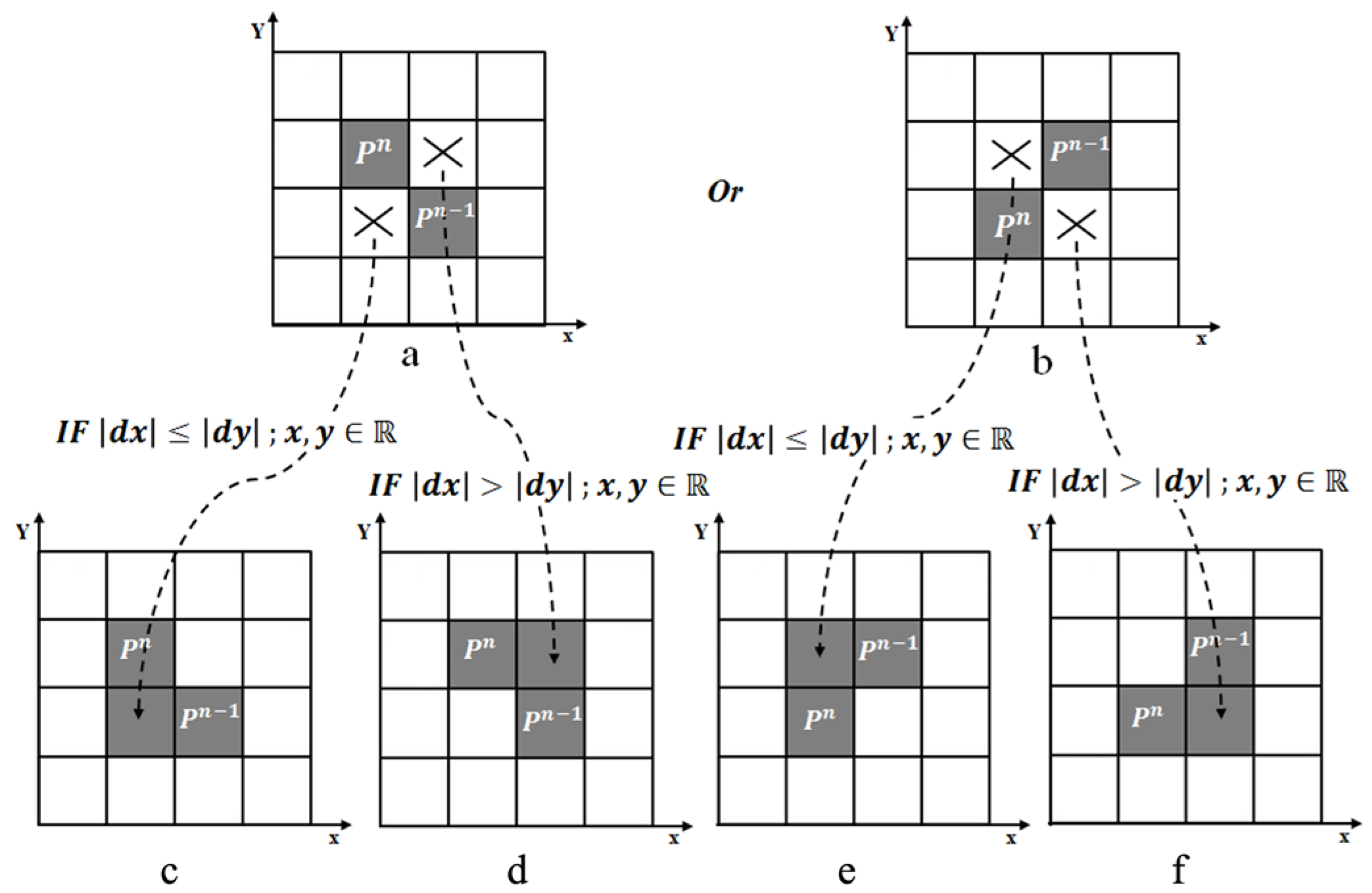
2.1.4. Post-Processing

In this section, some modifications are applied to the retrieved ${\mathit{r}}_x$ and ${\mathit{r}}_y$ signals to ensure their values can be embedded into the image plane. Additionally, paired samples of ${\mathit{r}}_x$ and ${\mathit{r}}_y$ that need to satisfy the condition ${\mathit{D}}^{\prime }\mathit{r}=0$ are detected and adjusted accordingly.

First, the positions of the snake points are determined using the sample values from the reconstructed ${\mathit{r}}_x$ and ${\mathit{r}}_y$ signals. These positions are represented as a set of coordinates: $\mathit{P}=\left\{\left({\mathit{r}}_x^1,{\mathit{r}}_y^1\right),\dots ,\left({\mathit{r}}_x^n,{\mathit{r}}_y^n\right)\right\}$. Here, ${\mathit{r}}_x^n$ and ${\mathit{r}}_y^n$ denote the n-th sample values of the ${\mathit{r}}_x$ and ${\mathit{r}}_y$ signals, respectively.

Second, to embed the members of $\mathit{P}$ into the image plane, the values of $\mathit{P}$ must be rounded to integers. However, rounding may lead to a diagonal neighbourhood between successive points, which must be corrected to ensure a 4-connected neighbourhood. To solve this problem, first, diagonal neighbours are detected using Euclidean distance i.e., $D=\sqrt{{({\mathit{P}}_x^n-{\mathit{P}}_x^{n-1})}^2+{({\mathit{P}}_y^n-{\mathit{P}}_y^{n-1})}^2}$, for $D>1$. To address the diagonal neighbourhood and transform it into a 4-connected neighbourhood, an intermediate snake point is inserted between the diagonally connected snake points. The adjustment can be performed in two ways, depending on the specific configuration of the diagonal connection. This is illustrated in Figure 7a,b. To decide the proper intermediate snake points for converting diagonal connections into 4-connected connections, the relative differences in the X- and Y-coordinates of the diagonally connected snake points are compared. To decide the proper intermediate snake points for converting the diagonal neighbourhood into a 4-connected neighbourhood, $dx={\mathit{c}}_x^n-{\mathit{c}}_x^{n-1}$ and $dy={\mathit{c}}_y^n-{\mathit{c}}_y^{n-1}$ of diagonally connected snake points are compared. If $\left|dx\right|\le \left|dy\right|$, the snake point is chosen in the way $x_{\times }={\mathit{P}}_x^{n-1}$ and $y_{\times }={\mathit{P}}_y^{n-1}+1$ as shown in Figure 7c,e. Otherwise, if $\left|dx\right|>\left|dy\right|$, $x_{\times }={\mathit{P}}_x^{n-1}+1$ and $y_{\times }={\mathit{P}}_y^{n-1}$ (Figure 7d,f). The algorithm for this step is detailed as Algorithm A1 in the Appendix A.

Figure 7. Transformation of diagonal connection of snake points to a 4-connected one. (a,b): Two possible configurations for the diagonal connection. (c): converting (a) to a 4-connected connection when $\left|dx\right|\le \left|dy\right|$, (d): converting (a) to a 4-connected connection when $\left|dx\right|>\left|dy\right|$, (e): converting (b) to a 4-connected connection when $\left|dx\right|\le \left|dy\right|$, (f): converting (b) to a 4-connected connection when $\left|dx\right|>\left|dy\right|$.

2.2. Splitting

After transforming the snake to a fully 4-connected contour, all self-loops within the contour are identified and extracted as separate contours using a straightforward algorithm. The process begins by plotting the resultant fully 4-connected snake onto an image matrix. Subsequently, intersecting snake points are identified at locations where snake points are plotted multiple times within the same array position. Upon detecting a crossing location, the snake points from the first occurrence of the intersection point (denoted as ${\mathit{P}}_k^{i_F}$) to the point just before the second occurrence of the same intersection point (denoted as ${\mathit{P}}_k^{i_S-1}$) are isolated and reassigned to form a new, separate snake. The algorithm iteratively examines the snakes for additional crossing locations and applies the same procedure until no further intersections are detected. The algorithm of the splitting process is detailed as Algorithm A2 in the Appendix A.

2.3. Merging

This section presents a novel algorithm designed to extract all closed loops formed after the collision of two or more separated snakes. For clarity, we illustrate the algorithm using Figure 8, where the white circles (i.e., $i_1=\left(x_1,y_1\right)\in {\mathit{P}}_k\cap {\mathit{P}}_{k+1}$ to $i_8=\left(x_8,y_8\right)\in {\mathit{P}}_k\cap {\mathit{P}}_{k+1}$) represent the crossing points. The problem of merging collided snakes can be subdivided into the extraction of two distinct types of snakes: (1) the outline or external snake (Figure 8, red dashed line 1), and (2) the internal snakes (Figure 8, red dashed lines 2, 3, and 4). The extraction of these internal and external snakes is discussed in the subsequent subsections.

Figure 8. An example of the occlusion of two snakes.

Before delving into the extraction process, we first introduce three key concepts. To accurately extract both external and internal snakes, the relative positions of the crossing points within each snake must be known. To achieve this, we define two “snake vectors”, which consists of each snake’s points arranged in sequence. Figure 9 illustrates two different contour vectors of the black snake in Figure 8. Furthermore, as shown in Figure 9, two types of paths, “Long Path” (LP) and “Short Path” (SP), can be defined within the snake vector based on the chosen starting point and the direction of traversal (clockwise or counterclockwise), illustrated by solid and dashed blue lines for crossing points of $i_2$ and $i_3$. In Figure 9a, the SP passes through both the beginning and end of the snake vector, while the LP does not. In contrast, Figure 9b demonstrates the inverse relationship between the SP and LP.

Figure 9. Two different statuses for LP and SP in snake vectors of the black contour in Figure 8. (a) SP passes the beginning and end of the snake vector while LP does not. (b) LP passes the beginning and end of the snake vector while SP does not.

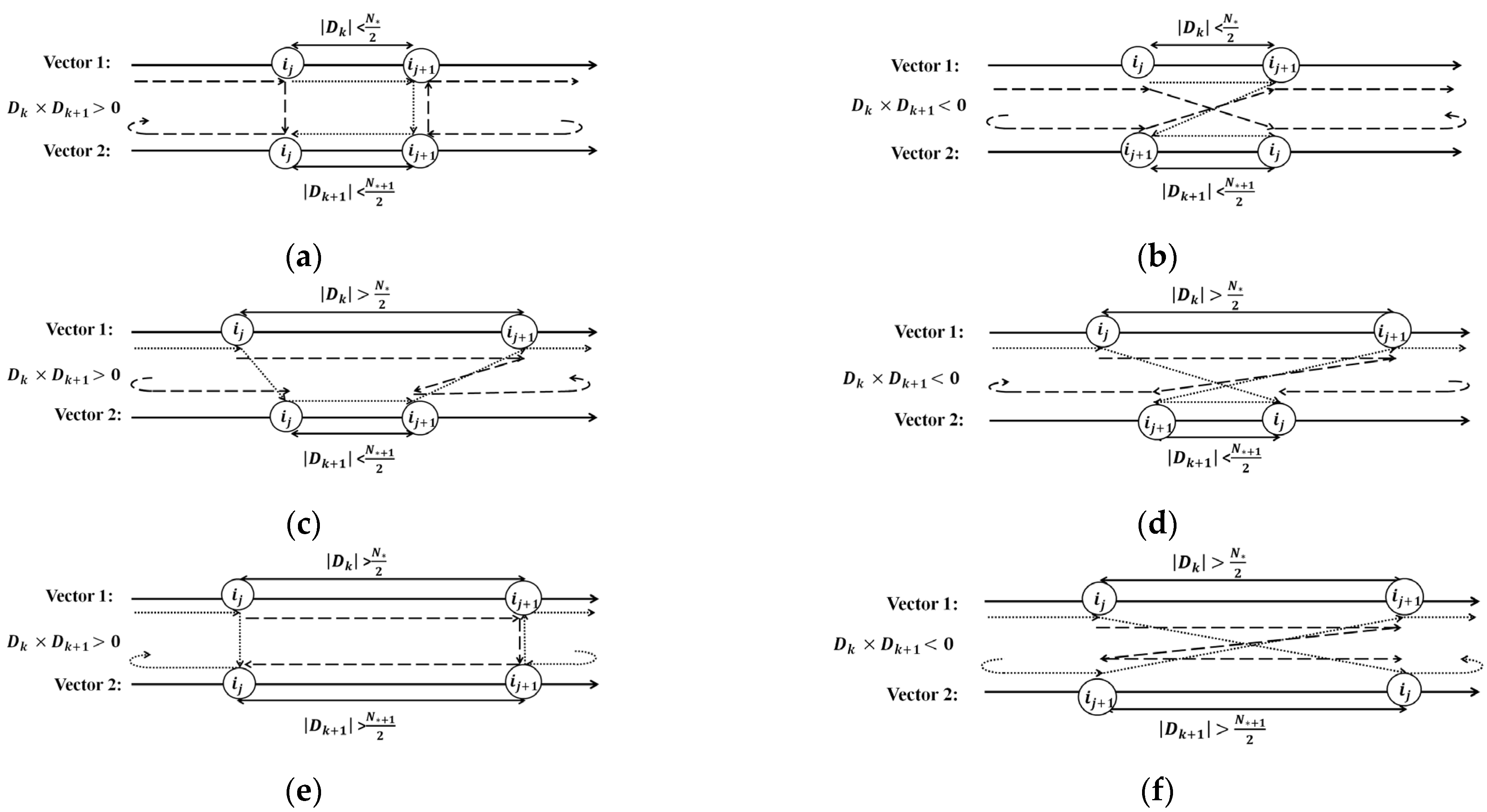
2.3.1. Extracting Internal Contours

To extract internal snakes, the first step is to select two successive, non-adjacent crossing points, such as $i_2$ and $i_3$(with $i_1$ and $i_2$being successive and adjacent). Next, the snake points that lie along the SPs between selected crossing points (depicted by the blue dotted lines in Figure 8) are extracted as part of the internal snake. This process is repeated for all successive, non-adjacent pairs of crossing points. There are six distinct configurations for extracting points along the SPs, depending on the choice of starting point for each snake vector: if both are in LPs, both are in SPs, or one is in LP and another in SP. For example, consider the crossing points $i_2$and $i_3$. If both starting points are in LPs, e.g., point “A” in Figure 8, and the black snake is mapped clockwise while the grey snake is mapped counterclockwise (or vice versa) into the snake vectors, this results in the configuration shown in Figure 10a. If both snakes are mapped into the snake vectors in the same direction (either both clockwise or both counterclockwise), the result corresponds to Figure 10b. If both crossing points are in SPs, e.g., “B”, with the black snake mapped clockwise and the grey snake mapped counterclockwise (or vice versa) into the snake vectors, the extraction status corresponds to Figure 10c, while the same direction for both contours (either clockwise or counterclockwise) results in the configuration shown in Figure 10d. Lastly, if one crossing point is in LP and another in SP, e.g., “C”, with the black snake mapped clockwise and the grey snake mapped counterclockwise (or vice versa) into the snake vectors, the configuration in Figure 10e is obtained, and when both snakes are mapped in the same direction, the configuration is as shown in Figure 10f.

Figure 10. Six different configurations for extracting LP (big dashed arrows) for external snake extraction and SP (small dashed arrows) for internal snake extraction. (a): $\left|D_k\right|<{\displaystyle \frac{N_k}{2}}$, $\left|D_{k+1}\right|<{\displaystyle \frac{N_{k+1}}{2}}$, and $D_{k+1}\times D_k>0$; (b): $\left|D_k\right|<{\displaystyle \frac{N_k}{2}}$, $\left|D_{k+1}\right|<{\displaystyle \frac{N_{k+1}}{2}}$, and $D_{k+1}\times D_k<0$; (c): $\left|D_k\right|>{\displaystyle \frac{N_k}{2}}$, $\left|D_{k+1}\right|<{\displaystyle \frac{N_{k+1}}{2}}$, and $D_{k+1}\times D_k>0$; (d): $\left|D_k\right|>{\displaystyle \frac{N_k}{2}}$, $\left|D_{k+1}\right|<{\displaystyle \frac{N_{k+1}}{2}}$, and $D_{k+1}\times D_k<0$; (e): $\left|D_k\right|>{\displaystyle \frac{N_k}{2}}$, $\left|D_{k+1}\right|>{\displaystyle \frac{N_{k+1}}{2}}$, and $D_{k+1}\times D_k>0$; (f): $\left|D_k\right|>{\displaystyle \frac{N_k}{2}}$, $\left|D_{k+1}\right|>{\displaystyle \frac{N_{k+1}}{2}}$, and $D_{k+1}\times D_k<0$.

To distinguish between each of the six configurations shown in Figure 10, we define the function $D_k=L_k\left(i_{j+1}\right)-L_k\left(i_j\right)$, where $L$ gives the index of the snake point within the snake vector, and $i_{j+1}$ and $i_j$ are two successive and non-adjacent crossing points. For each snake, if $\left|D_k\right|>{\displaystyle \frac{N_k}{2}}$ (where $N_k$ represents the total number of points in each snake vector), the SP passes through both the beginning and end of the snake vector. This situation corresponds to vector 1 in Figure 10c,d, as well as both vectors in Figure 10e,f. Conversely, if $\left|D_k\right|<{\displaystyle \frac{N_k}{2}}$, the SP does not pass through the beginning and end of the snake vector. This case corresponds to vector 2 in Figure 10c,d, as well as both vectors in Figure 10a,b. Additionally, the sign of the product $D_{k+1}\times D_k$ determines the direction of mapping snake points, i.e., clockwise or counterclockwise, in the snake vectors. Specifically:

• If $D_{k+1}\times D_k>0$, the sequence of the two crossing points in both vectors is either clockwise or counterclockwise (Figure 10a,c,e).
• If $D_{k+1}\times D_k<0$, the sequence of the crossing points differs, i.e., one is clockwise while another one is counterclockwise (Figure 10b,d,f).

Based on the output of the function $D$, the SP for each of the six statuses can be identified and extracted, as illustrated by the small dashed lines in Figure 10. Algorithm A3, presented in Appendix A, formalises the process of extracting internal snakes after the collision of two or more snakes.

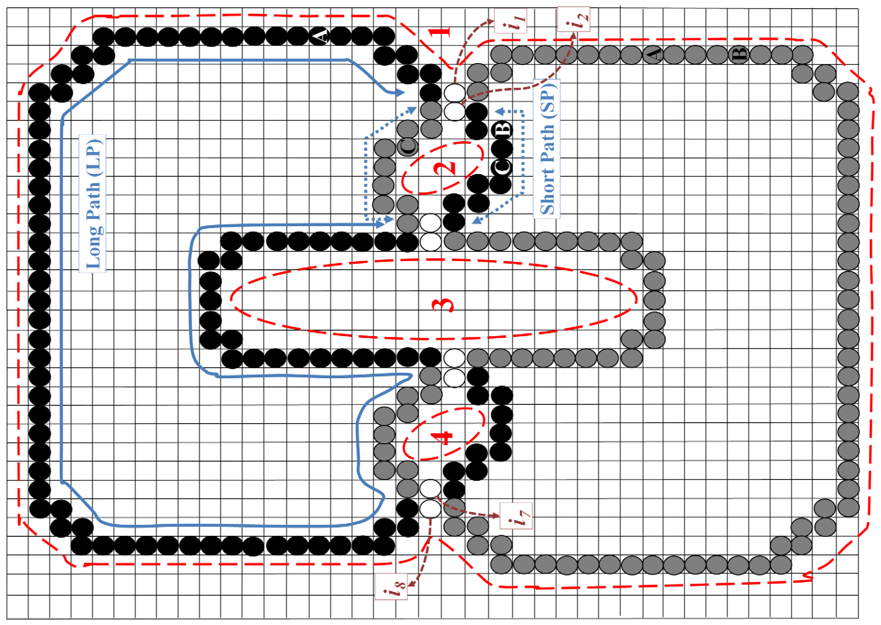
2.3.2. Merging External Contours

To extract the external contour, the process begins by identifying two outer crossing points, i.e., $i_1$ and $i_8$. These points are then used to extract the snake points that lie along the LPs between $i_1$ and $i_8$ (illustrated by the solid blue line in Figure 8), forming the external contour. To detect the pair of outer crossing points, in our example $i_1$ and $i_8$, SPs between crossing points are evaluated two-by-two, and the pair of crossing points with the longest SP is selected as the outer crossing points. To extract LPs, there are six configurations presented in Figure 10 by the large dashed arrows. The sign of $D_{k+1}\times D_k$ retains the same interpretation as discussed in Section 2.3.1. However, the value of $\left|D_k\right|$ has a different meaning for LP extraction. Specifically:

• If $\left|D_k\right|<{\displaystyle \frac{N_k}{2}}$, the LP passes through the beginning and end of the snake vector. This is represented by vector 2 in Figure 10c,d, as well as both vectors in Figure 10a,b.
• If $\left|D_{k }\right|>{\displaystyle \frac{N_k}{2}}$, the LP does not pass through the beginning and end of the contour vector. This corresponds to vector 1 in Figure 10c,d, and both vectors in Figure 10e,f.

Algorithm A4, presented in Appendix A, provides a detailed methodology for extracting the external contour after the collision of two or more snakes.

Below, we present the steps outlining how to plug or integrate the proposed splitting and merging algorithm into an image segmentation process using a snake algorithm:

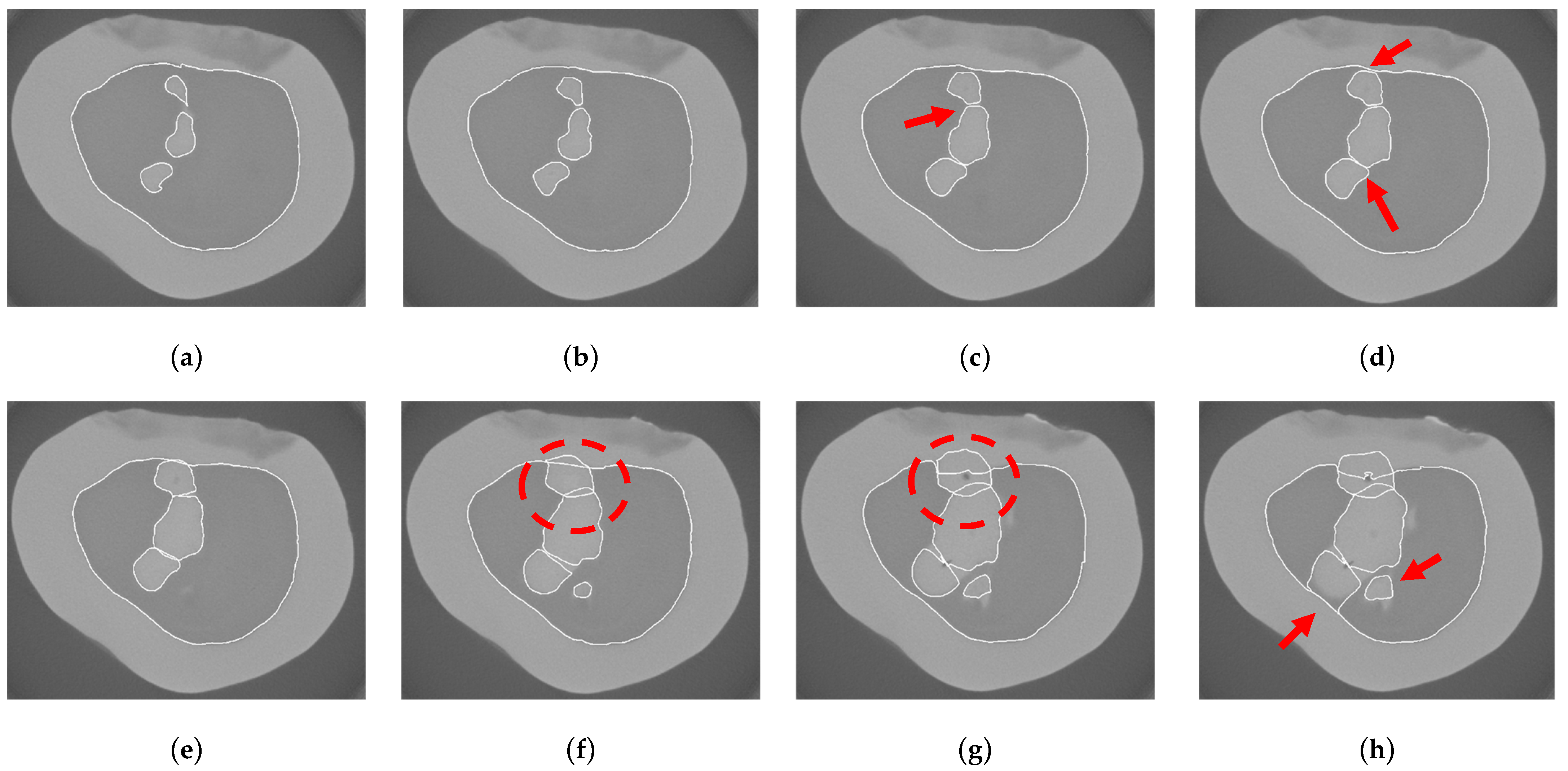
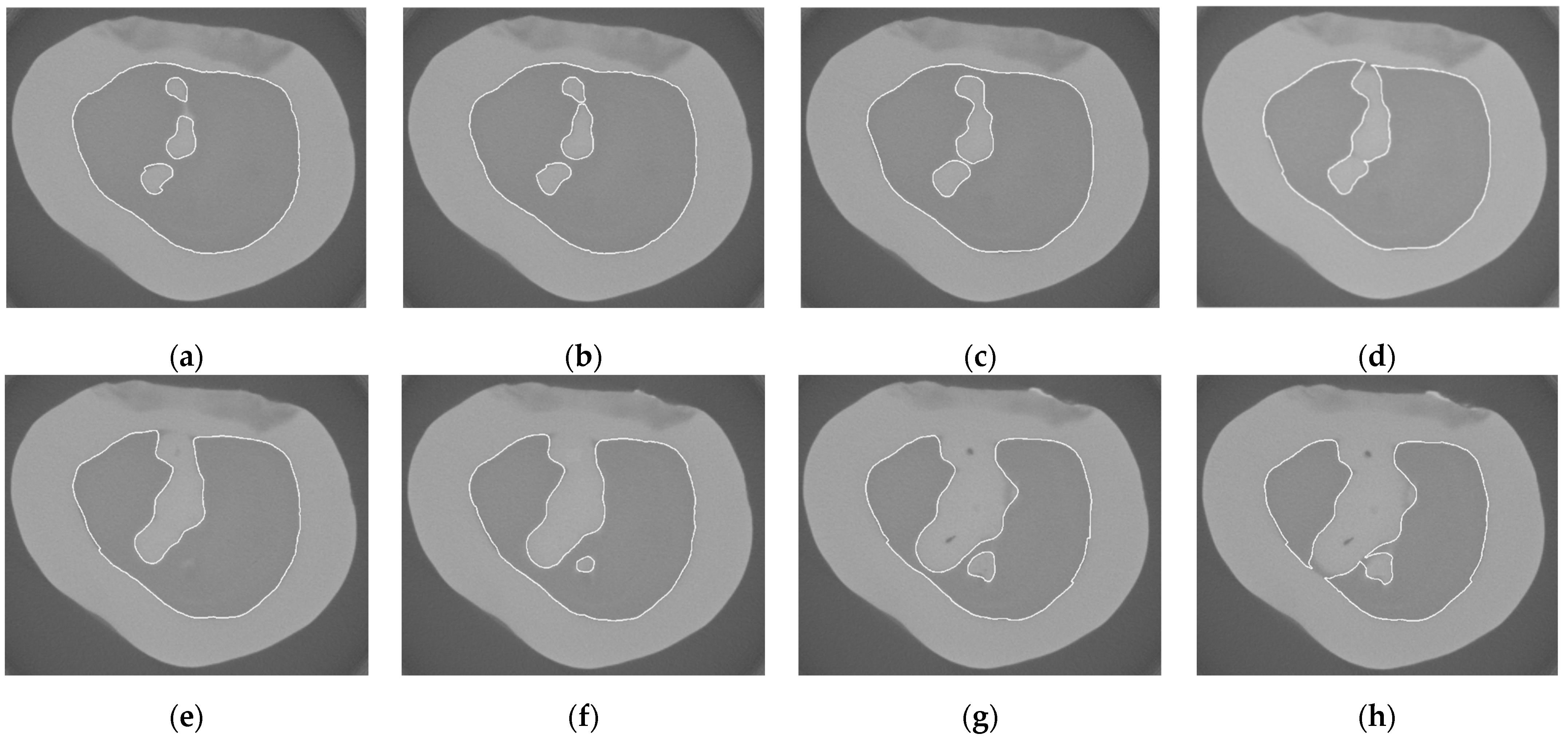
• The locations of snakes in the initial image are manually defined.
• The boundaries are detected using the AC model.
• The resultant boundaries are converted into fully 4-connected contours.
• These fully 4-connected contours are passed through the splitting algorithm, where contours with fewer than 50 points, identified as self-loops, are removed.
• The merging algorithm then processes the remaining contours to identify and merge collided contours.
• Finally, the output contour from the merging algorithm serves as the initial positions for the snakes in the next image, and the process is repeated.

3. Results

This section demonstrates the performance of the proposed algorithm for splitting and merging of the snakes through two experiments.

The first experiment aims to detect the boundary between the dentin (dark grey region in Figure 11) and enamel (light grey region in Figure 11) in sequential 2D images from a tooth Micro-computed tomography (Micro-CT) dataset using a snake. Browsing 2D images of this 3D dataset sequentially exhibit anatomical variations that lead to the splitting and merging of enamel regions in Figure 11. For this experiment, we use a dataset consisting of Micro-CT images of a tooth, described in [47]. In the process of boundary detection, each detected contour in a 2D image serves as the initial position of the snakes in the subsequent image. By applying the proposed splitting and merging method, we effectively regulate topology changes in the snakes, ensuring accurate and adaptive boundary detection.

Figure 11. Results of applying the original snake without proposed splitting and merging method to detect enamel’s boundaries in successive images of 3D Micro-CT. In (a), four snakes begin their evolution, and continue at (b). The first merging is expected to occur at (c), indicated by the red arrow, however, without the splitting and merging algorithm, snakes cannot merge or split. Similarly, in the following image at (d), two additional merges (shown by red arrows) cannot be processed. Then, the snakes continue evolution at (e–g). As shown by red circles at (f,g), the lack of splitting and merging leads to an inaccurate edge detection. Finally, at (h), two more topological changes are expected but cannot be handled without the proposed algorithm.

Before initiating boundary detection using the snake, we perform image denoising as a preprocessing step using the total variation method [48,49]. Micro-CT images inherently contain significant noise, which poses challenges for snakes in accurately detecting boundaries. After noise reduction, the boundary between enamel and dentin regions is detected using a snake implemented by MATLAB, version R2024b, as explained at the end of the method section.

To underscore the importance of splitting and merging in snakes, Figure 11 presents the results of the original snake without implementing the proposed splitting and merging approach, whereas Figure 12 shows the results after applying the proposed method. As shown in Figure 11a, in the initial 2D image, four separate contours are detected in the image. The boundary detection then continues sequentially, image by image, until the first merging is expected to occur in Figure 11c, as indicated by the red arrow. Using the proposed method, two internal snakes merge, and the number of snakes is reduced to three, as observed in Figure 12c. Similarly, in Figure 12d, our proposed algorithm successfully performs two merges. In addition, the lack of topology handling results in inaccurate edge detection in the next images, such as the red dashed circles in Figure 11f,g. Finally, in Figure 12h, the proposed method successfully handles the expected splitting and merging as indicated by red arrows in Figure 11h.

Figure 12. Results of integrating the proposed splitting and merging method with the snake algorithm to handle topology changes in the images from Figure 11. Compared to the corresponding images in Figure 11, the proposed algorithm successfully manages the merging and splitting of snakes, effectively handling the topological changes. As shown at (a,b), four snakes evolve similar to Figure 11a,b. Then, first merging occurs at (c), followed by two additional merges at (d). Subsequently, the snake continues to evolve at (e–g). Finally, one merging and one splitting occur at (h).

In the second experiment, we detect the lumens of coronary arteries in 2D images from a cardiac CT dataset using the snake sequentially, where the detected contour in each 2D image serves as the initial position of the snake in the next image. The dataset used in this experiment is freely available, and further details can be found in [50]. Browsing through the sequential 2D images of this 3D dataset reveals the merging of lumen cross-sections, which corresponds to the joining of different artery branches in 3D. To detect the lumen boundaries, we follow the same procedure as in the first experiment for detecting the boundary between enamel and dentin. Figure 13 and Figure 14 show the results of snake’s edge detection without and with the proposed splitting and merging algorithm. As shown in Figure 13a, in the initial 2D image, four lumens are detected by the snakes. As the snakes evolve sequentially through the images, the first merging is expected in Figure 13b, indicated by the red arrow, which is resolved using the proposed method in Figure 14b. Similarly, the unresolved merges (shown by red arrows) in Figure 13c are processed in Figure 14c. Finally, the last merging expected in Figure 13g is successfully resolved by the proposed method in Figure 14g.

Figure 13. Results of applying the original snake without proposed splitting and merging method to detect lumens’ boundaries. In (a), four snakes (red contours) begin their evolution, with the first expected merging at (b), indicated by the red arrow. Without the splitting and merging algorithm, the snakes cannot merge or split. Similarly, in the following image at (c), one additional merge (shown by red arrow) cannot be processed. Then, four snakes continue to evolve at (d–f). Finally, at (g), another merging is expected but cannot occur without the proposed algorithm. These snakes overlap without merging, as shown at (h).

Figure 14. Results of integrating the proposed splitting and merging method with the snake algorithm to handle topology changes in the images from Figure 13. Compared to the corresponding images in Figure 13, the proposed algorithm successfully manages the merging and splitting of snakes, effectively handling the topological changes. At (a) four snakes (red contours) are detected. The first and second merging happen at (b,c). Then, two snakes continue to evolve at (d–f). Finally, the last merging occurs at (g), after which a snake continues its evolution, as shown at (h).

Finally, to further assess self-loops removal, we conduct a third experiment introducing larger self-loops during initialisation, the green contour in Figure 15. The splitting method effectively removes these loops, as shown in Figure 15, with different colours illustrating results of snake evolution at each iteration.

Figure 15. Performance of splitting algorithm for self-loops removal. The green contour shows the initial contour. Results of applying the splitting algorithm for each iteration are depicted by different colours sequentially.

Performance-wise, the proposed algorithm added less than 8% runtime overhead to the original snake for handling topology changes in the first and second experiments. In the third experiment, detecting and removing self-loops increased runtime by approximately 4%, highlighting the algorithm’s efficiency and effectiveness in handling self-crossing occurrence in the complex topology changes.

4. Conclusions

In this paper, we proposed a novel method for handling topology changes in snakes (parametric ACs). Our approach effectively manages the splitting and merging of snakes through three stages: fully 4-connected interpolation, snake splitting, and snake merging, ensuring improved robustness in snake evolution.

To evaluate our method, we applied it to both dental Micro-CT and cardiac CT datasets to detect the boundary of enamel and artery lumens, respectively, demonstrating its ability to accurately handle complex topological changes. The results confirm that our method successfully preserves snake integrity, though it introduces a moderate increase in runtime.

This advancement is significant because topology changes are a major challenge in snake models, particularly in medical image segmentation, where anatomical structures frequently split and merge. By addressing these challenges, our method enhances the accuracy and adaptability of snakes, making them more reliable for medical imaging and other applications requiring dynamic boundary detection.

The proposed splitting and merging method has demonstrated its effectiveness in boundary detection in CT imaging. Future work should explore its application to other imaging modalities, such as MRI, ultrasound, and PET, where boundary detection challenges differ, particularly in terms of tissue complexity.

Additionally, we aim to optimise the algorithm in the future to reduce computational overhead and explore its integration with deep learning-based AC models, such as DeepSnake. Since learning-based AC models are trained to predict energy terms or forces, they guide the contour through multiple iterations to achieve an optimal shape. Therefore, similar to traditional AC models, the proposed splitting and merging approach can detect and resolve potential collisions at the end of each iteration. Finally, extending our method to 3D ACs could further enhance its applicability in volumetric image analysis.

References

- Jing, J.; Liu, S.; Wang, G.; Zhang, W.; Sun, C. Recent advances on image edge detection: A comprehensive review. Neurocomputing 2022, 503, 259–271. [Google Scholar] [CrossRef]
- Kass, M.; Witkin, A.; Terzopoulos, D. Snakes: Active contour models. Int. J. Comput. Vis. 1988, 1, 321–331. [Google Scholar] [CrossRef]
- Peng, S.; Jiang, W.; Pi, H.; Li, X.; Bao, H.; Zhou, X. Deep snake for real-time instance segmentation. In Proceedings of the IEEE/CVF Conference on Computer Vision and Pattern Recognition, Seattle, WA, USA, 13–19 June 2020. [Google Scholar]
- Caselles, V.; Kimmel, R.; Sapiro, G. Geodesic active contours. In Proceedings of the Fifth International Conference on Computer Vision, Cambridge, MA, USA, 20–23 June 1995; pp. 694–699. [Google Scholar]
- Malladi, R.; Sethian, J.A.; Vemuri, B.C. Shape modeling with front propagation: A level set approach. IEEE Trans. Pattern Anal. Mach. Intell. 1995, 17, 158–175. [Google Scholar] [CrossRef]
- Sapiro, G.; Tannenbaum, A. Affine invariant scale-space. Int. J. Comput. Vis. 1993, 11, 25–44. [Google Scholar] [CrossRef]
- Osher, S.; Sethian, J.A. Fronts propagating with curvature-dependent speed: Algorithms based on Hamilton-Jacobi formulations. J. Comput. Phys. 1988, 79, 12–49. [Google Scholar] [CrossRef]
- McInerney, T.; Terzopoulos, D. T-snakes: Topology adaptive snakes. Med. Image Anal. 2000, 4, 73–91. [Google Scholar] [CrossRef]
- Xu, C.; Pham, D.L.; Prince, J.L. Image segmentation using deformable models. Handb. Med. Imaging 2000, 2, 129–174. [Google Scholar]
- Chan, T.F.; Vese, L.A. Active contours without edges. IEEE Trans. Image Process. 2001, 10, 266–277. [Google Scholar] [CrossRef]
- Samson, C.; Blanc-Féraud, L.; Zerubia, J.; Aubert, G. A level set model for image classification. In Proceedings of the International Conference on Scale-Space Theories in Computer Vision, Corfu, Greece, 26–27 September 1999; pp. 306–317. [Google Scholar]
- Yezzi, A.; Tsai, A.; Willsky, A. A statistical approach to snakes for bimodal and trimodal imagery. In Proceedings of the Seventh IEEE International Conference on Computer Vision, Kerkyra, Greece, 20–27 September 1999; pp. 898–903. [Google Scholar]
- Delingette, H.; Montagnat, J. Shape and topology constraints on parametric active contours. Comput. Vis. Image Underst. 2001, 83, 140–171. [Google Scholar] [CrossRef]
- Bischoff, S.; Kobbelt, L. Snakes with topology control. Vis. Comput. 2003, 20, 217–228. [Google Scholar]
- Bischoff, S.; Kobbelt, L.P. Parameterization-free active contour models with topology control. Vis. Comput. 2004, 20, 217–228. [Google Scholar]
- Oliveira, A.; Ribeiro, S.; Farias, R.; Esperança, C. Loop snakes: Snakes with enhanced topology control. In Proceedings of the 17th Brazilian Symposium on Computer Graphics and Image Processing, Curitiba, Brazil, 20 October 2004; pp. 364–371. [Google Scholar]
- Oliveira, A.; Ribeiro, S.; Esperanca, C.; Giraldi, G. Loop snakes: The generalized model. In Proceedings of the Ninth International Conference on Information Visualisation, London, UK, 6–8 July 2005; pp. 975–980. [Google Scholar]
- Zheng, S. An intensive restraint topology adaptive snake model and its application in tracking dynamic image sequence. Inf. Sci. 2010, 180, 2940–2959. [Google Scholar] [CrossRef]
- Ivins, J.; Porrill, J. Active region models for segmenting textures and colours. Image Vis. Comput. 1995, 13, 431–438. [Google Scholar] [CrossRef]
- Ďurikovič, R.; Kaneda, K.; Yamashita, H. Dynamic contour: A texture approach and contour operations. Vis. Comput. 1995, 11, 277–289. [Google Scholar] [CrossRef]
- Wong, Y.; Yuen, P.C.; Tong, C.S. Segmented snake for contour detection. Pattern Recognit. 1998, 31, 1669–1679. [Google Scholar] [CrossRef]
- Choi, W.-P.; Lam, K.-M.; Siu, W.-C. An adaptive active contour model for highly irregular boundaries. Pattern Recognit. 2001, 34, 323–331. [Google Scholar] [CrossRef]
- Lefèvre, S.; Vincent, N. Real time multiple object tracking based on active contours. In Proceedings of the International Conference Image Analysis and Recognition, Porto, Portugal, 29 September–1 October 2004; pp. 606–613. [Google Scholar]
- Li, C.; Liu, J.; Fox, M.D. Segmentation of external force field for automatic initialization and splitting of snakes. Pattern Recognit. 2005, 38, 1947–1960. [Google Scholar] [CrossRef]
- Xingfei, G.; Jie, T. An automatic active contour model for multiple objects. In Proceedings of the 16th International Conference on Pattern Recognition, Quebec City, QC, Canada, 11–15 August 2002; pp. 881–884. [Google Scholar]
- Chuang, C.-H.; Lie, W.-N. Automatic snake contours for the segmentation of multiple objects. In Proceedings of the 2001 IEEE International Symposium on Circuits and Systems, Sydney, NSW, Australia, 6–9 May 2001; pp. 389–392. [Google Scholar]
- De Berg, M.; Van Kreveld, M.; Overmars, M.; Schwarzkopf, O.C. Computational geometry. In Computational Geometry; Springer: Berlin/Heidelberg, Germany, 2000; pp. 1–17. [Google Scholar]
- Cohen, J.D.; Lin, M.C.; Manocha, D.; Ponamgi, M. I-collide: An interactive and exact collision detection system for large-scale environments. In Proceedings of the 1995 Symposium on Interactive 3D Graphics, Monterey, CA, USA, 9–12 April 1995; pp. 189–ff. [Google Scholar]
- Smith, C.E.; Schaub, H. Efficient polygonal intersection determination with applications to robotics and vision. In Proceedings of the 2005 IEEE/RSJ International Conference on Intelligent Robots and Systems (IROS 2005), Edmonton, AB, Canada, 2–6 August 2005; pp. 3890–3895. [Google Scholar]
- Perrin, D.P.; Ladd, A.M.; Kavraki, L.E.; Howe, R.D.; Cannon, J.W. Fast intersection checking for parametric deformable models. In Proceedings of the Medical Imaging, San Diego, CA, USA, 13–17 February 2005; pp. 1468–1474. [Google Scholar]
- Doğan, G.; Morin, P.; Nochetto, R.H. A variational shape optimization approach for image segmentation with a Mumford–Shah functional. SIAM J. Sci. Comput. 2008, 30, 3028–3049. [Google Scholar] [CrossRef]
- Stoeter, S.A.; Papanikolopoulos, N. Closed dynamic contour models that split and merge. In Proceedings of the ICRA’04: 2004 IEEE International Conference on Robotics and Automation, New Orleans, LA, USA, 26 April–1 May 2004; pp. 3883–3888. [Google Scholar]
- Pauš, P.; Beneš, M. Algorithm for topological changes of parametrically described curves. In Proceedings of the ALGORITMY 2009: 18th Conference on Scientific Computing, Vysoké Tatry, Slovakia, 15–20 March 2009; pp. 176–184. [Google Scholar]
- Araki, S.; Yokoya, N.; Iwasa, H.; Takemura, H. Splitting of active contour models based on crossing detection for extraction of multiple objects. Syst. Comput. Jpn. 1997, 28, 34–42. [Google Scholar] [CrossRef]
- Araki, S.; Yokoya, N.; Takemura, H. Real-time tracking of multiple moving objects using split-and-merge contour models based on crossing detection. Syst. Comput. Jpn. 1999, 30, 25–33. [Google Scholar] [CrossRef]
- Ngoi, K.P.; Jia, J. An active contour model for colour region extraction in natural scenes. Image Vis. Comput. 1999, 17, 955–966. [Google Scholar] [CrossRef]
- Nakaguro, Y.; Makhanov, S.S.; Dailey, M.N. Numerical experiments with cooperating multiple quadratic snakes for road extraction. Int. J. Geogr. Inf. Sci. 2011, 25, 765–783. [Google Scholar] [CrossRef]
- Rochery, M.; Jermyn, I.H.; Zerubia, J. Higher order active contours. Int. J. Comput. Vis. 2006, 69, 27–42. [Google Scholar] [CrossRef]
- Mikula, K.; Urbán, J. New fast and stable Lagrangean method for image segmentation. In Proceedings of the 2012 5th International Congress on Image and Signal Processing (CISP), Chongqing, China, 16–18 October 2012; pp. 688–696. [Google Scholar]
- Balažovjech, M.; Mikula, K.; Petrášová, M.; Urbán, J. Lagrangean method with topological changes for numerical modelling of forest fire propagation. In Proceedings of the ALGORITMY 2012: 19th Conference on Scientific Computing, Vysoké Tatry, Slovakia, 9–14 September 2015; pp. 42–52. [Google Scholar]
- Benninghoff, H.; Garcke, H. Efficient image segmentation and restoration using parametric curve evolution with junctions and topology changes. SIAM J. Imaging Sci. 2014, 7, 1451–1483. [Google Scholar] [CrossRef]
- Benninghoff, H.; Garcke, H. Image Segmentation Using Parametric Contours with Free Endpoints. IEEE Trans. Image Process. 2016, 25, 1639–1648. [Google Scholar] [CrossRef]
- Ji, L.; Yan, H. Loop-free snakes for highly irregular object shapes. Pattern Recognit. Lett. 2002, 23, 579–591. [Google Scholar] [CrossRef]
- Ji, L.; Yan, H. Robust topology-adaptive snakes for image segmentation. Image Vis. Comput. 2002, 20, 147–164. [Google Scholar] [CrossRef]
- Nakhmani, A.; Tannenbaum, A. Self-crossing detection and location for parametric active contours. IEEE Trans. Image Process. 2012, 21, 3150–3156. [Google Scholar] [CrossRef]
- Lashgari, M.; Rabbani, H.; Plonka, G.; Selesnick, I. Reconstruction of Connected Digital Lines Based on Constrained Regularization. IEEE Trans. Image Process. 2022, 31, 5613–5628. [Google Scholar] [CrossRef]
- Lashgari, M.; Shahmoradi, M.; Rabbani, H.; Swain, M. Missing surface estimation based on modified tikhonov regularization: Application for destructed dental tissue. IEEE Trans. Image Process. 2018, 27, 2433–2446. [Google Scholar] [CrossRef]
- Lashgari, M.; Rabbani, H.; Shahmorad, M.; Swain, M. A fast and accurate dental micro-CT image denoising based on total variation modeling. In Proceedings of the 2015 IEEE Workshop on Signal Processing Systems (SiPS), Hangzhou, China, 14–16 October 2015; pp. 1–5. [Google Scholar]
- Shahmoradi, M.; Lashgari, M.; Rabbani, H.; Qin, J.; Swain, M. A comparative study of new and current methods for dental micro-CT image denoising. Dentomaxillofac. Radiol. 2016, 45, 20150302. [Google Scholar] [CrossRef] [PubMed]
- Gharleghi, R.; Adikari, D.; Ellenberger, K.; Webster, M.; Ellis, C.; Sowmya, A.; Ooi, S.; Beier, S. Annotated computed tomography coronary angiogram images and associated data of normal and diseased arteries. Sci. Data 2023, 10, 128. [Google Scholar] [CrossRef]
Disclaimer/Publisher’s Note: The statements, opinions and data contained in all publications are solely those of the individual author(s) and contributor(s) and not of MDPI and/or the editor(s). MDPI and/or the editor(s) disclaim responsibility for any injury to people or property resulting from any ideas, methods, instructions or products referred to in the content. |
© 2025 by the authors. Licensee MDPI, Basel, Switzerland. This article is an open access article distributed under the terms and conditions of the Creative Commons Attribution (CC BY) license (https://creativecommons.org/licenses/by/4.0/).