Abstract
This article presents the Transfer Matrix Method as a mathematical approach for the calculus of different structures that can be discretized into elements using an iterative calculus for future applications in the vehicle industry. Plate calculus is important in construction, medicine, orthodontics, and many other fields. This work is original due to the mathematical apparatus used in the calculus of long rectangular plates embedded in both long borders and required by a uniformly distributed force on a line parallel to the long borders. The plate is discretized along its length in unitary beams, which have the width of the rectangular plate. The unitary beam can also be discretized into parts. As applications, the long rectangular plates embedded on the two long borders and charged with a vertical uniform load that acts on a line parallel to the long borders are studied. A state vector is associated with each side. For each of the four cases studied, a matrix relationship was written for each side, based on a transfer matrix, the state vector corresponding to the origin side, and the vector due to the action of external forces acting on the considered side. After, it is possible to calculate all the state vectors for all sides of the unity beam. Now, the efforts, deformations, and stress can be calculated in any section of the beam, respectively, for the long rectangular plate. This calculus will serve as a calculus of resistance for different pieces of the components of vehicles.
Keywords:
long rectangle plate; unit beam; transfer matrix; state vector; charge density; Dirac’s function and operators; Heaviside’s function and operators; vehicle industry MSC:
74-10
1. Introduction
This study was conducted due to the need to calculate the resistance of plates for the vehicle industry. Vehicles are complex assemblies that have several components like plates. Plate calculus is not only important in the automobile industry, it is also important in construction, medicine, orthodontics, and many other fields. This work is original. The Transfer Matrix Method (TMM) is a mathematical approach to the calculus of different structures that can be discretized into elements using an iterative calculus, as in [1]. Classical Calculus of Material Resistance is presented in [2]. The authors of [3,4] give the calculus of a long cylinder tube for industrial applications by the TMM. An approach with the TMM for mandible body bone calculus is shown in [5]. The authors of [6] present the calculus through the TMM of a beam with intermediate support with applications in dental restorations. The authors of [7] present a triangular shell element for geometrically nonlinear analysis. The calculus of long rectangle plates articulated on both long sides charged with a linear load uniformly distributed on a line parallel to the long borders through the TMM is given in [8]. A simple triangular finite element for nonlinear thin shells: statics, dynamics, and anisotropy is shown in [9]. The authors of [10] present a simple geometrically exact finite element for thin shells in a static state. Meshless analysis of shear deformable shells: boundary and interface constraints are given in [11]. A continuity re-relaxed thin shell formulation for static and dynamic analyses of linear problems is shown in [12]. Another approach by the Finite Elements Method (FEM) applied for the calculus of rectangular plates is presented in [13,14]. The study of bending for a rectangular plate with each edge’s arbitrary point supported under a concentrated load is given in [15]. The authors of [16] present an analysis of folded plate structures by a combined Boundary Element–TMM and the authors of [17] present a FEM-TMM for dynamic analysis of frame structures. Elastic analysis and application tables of rectangular plates with unilateral contact support conditions are given in [18]. The authors of [19] present theoretical aspects for time–harmonic analysis of acoustic pulsation in gas pipeline systems using the FEM and TMM. The authors of [20] present an integrated TMM for multiple connected mufflers, and the authors of [21] present the determination of the stress–strain state in thin orthotropic plates on Winkler’s elastic foundations. An evaluation of a hybrid underwater sound-absorbing meta-structure by using the TMM is given in [22]. Some theoretical and experimental extensions based on the properties of the Intrinsic Transfer Matrix are presented in [23]. The TMM is applied to the parallel assembly of sound-absorbing materials in [24]. The authors of [25,26] use the TMM for multibodies in the past, present, and future and its applications. The authors of [27] present the muffler modeling by TMM and experimental verification. The authors of [28] present the development of the two-dimensional theory of thick plates bending based on the general solution of Lamé equations. A study of coupling the TMM to the FEM for analyzing the acoustics of complex hollow body networks is presented in [29]. Equivalent systems for the analysis of rectangular plates of varying thickness are shown in [30]. The classical theory of plates is presented in [31]. A study about the bending of clamped rectangular plates is given in [32]. The determination of plane stress and the strain of plates on the basis of the three-dimensional theory of elasticity is shown in [33]. Analysis of hypotheses used when constructing the theory of beams and plates is presented in [34]. The calculus of plates by the series representation of the deflection function is given in [35]. The authors of [36] present a solution of non-rectangular plates with the macro element method. The stress state of a compound polygonal plate is shown in [37]. The authors of [38] present a solution of thin rectangular plates with various boundary conditions and the authors of [39] present an exact solution for the deflection of a clamped rectangular plate under uniform load. The stress–strain state in the corner points of a clamped plate under a uniformly distributed normal load is given in [40], and a static analysis of an orthotropic plate is presented in [41]. The theory of plates and shells is given in [42]. A study about stress–strain analysis of rectangular plates with a variable thickness and constant weight is presented in [43] and an analysis of homogeneous and non-homogeneous plates is shown in [44]. A theoretical and comparative study regarding the mechanical response under the static loading for different rectangular plates is given in [45]. Approximate analytical solutions in the analysis of thin elastic plates are given in [46]. Some aspects of implementation of the boundary elements method in plate theory are presented in [47]. A convergence analysis of the finite element approach to the classical approach for analysis of plate bending is presented in [48]. Another study by a method of matched sections as a beam-like approach for plate analysis is presented in [49]. Application of the numerical methods in solving a phenomenon of the theory for thin plates is shown in [50]. A review of a few selected theories of plate bending is given in [51]. The authors of [52] present the calculus of plate–beam systems by the boundary elements method. Analytical solutions of the mechanical answer of thin orthotropic plates are shown in [53]. The Optimized Transfer Matrix approach for global buckling analysis with bypassing zero matrix inversion is given in [54]. The American Standard Test Method for the Measurement of Normal Incidence Sound Transmission of Acoustical Materials Based on the TMM from the American Society for Testing and Materials is presented in [55].
2. Calculus Premises Using the Transfer Matrix Method for Long Rectangular Plates
A rectangular plate with long lengths can be calculated using the TMM. The plate is discretized of its lengths into pieces, as in Figure 1a,b.
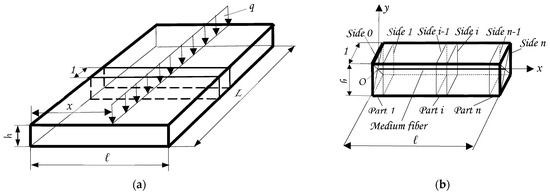
Figure 1.
Long rectangular plate and its discretization: (a) a long rectangle plate discretized into beams (pieces) with width equal at unity; (b) a unit beam (unit piece) discretized into n parts with n + 1 sides.
A piece (a beam) has the width equal to unity.
2.1. The State Vectors and the Transfer Matrix for a Long Rectangular Plate
2.1.1. State Vectors
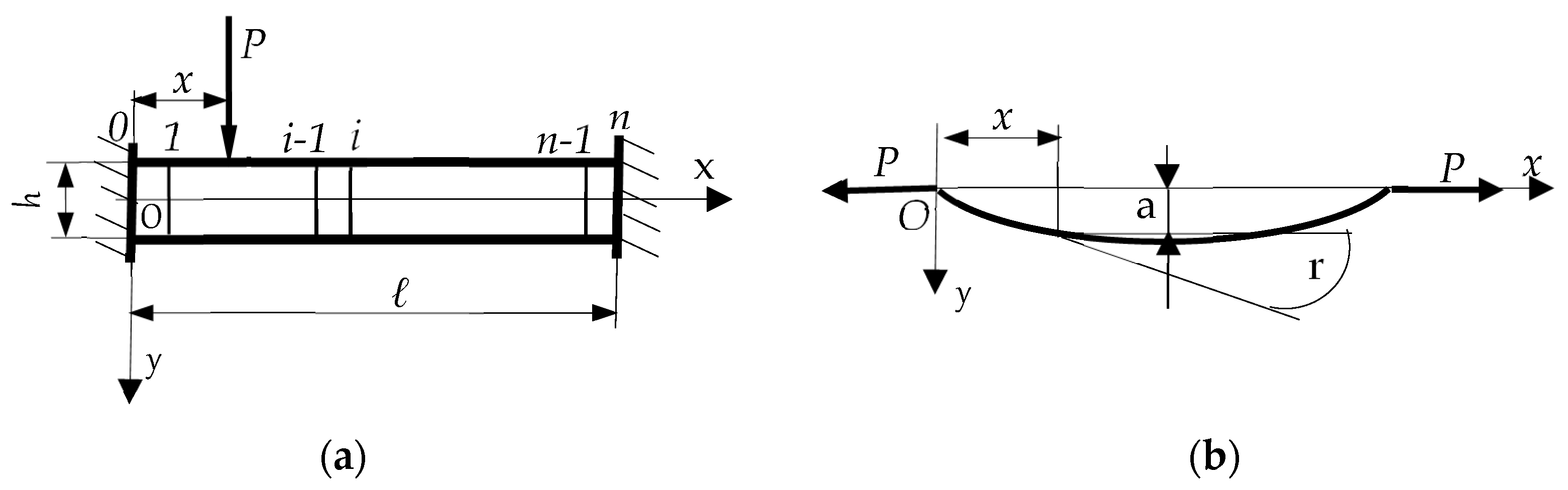
A unitary beam, with the width equal to unity, as in Figure 2a, can be associated with a Transfer Matrix. It is deformed, as in Figure 2b.

Figure 2.
A unitary beam (unitary piece): (a) unitary beam and the xOy reference system; (b) the average deformed fiber of the unitary beam.
Along its length, which is the width of the rectangular plate, the unitary beam can also be discretized into n parts (Figure 1b and Figure 2a). The sectioning of the beam is conducted perpendicularly to the Ox axis. Each part can be defined as the left side and a right side. For the first left part, it is defined as the left side, noted 0, and the right side, noted 1. The last right side of the last part n (on the right of the beam) is noted by n. So, the beam has n parts and n + 1 sides.
- -
- A state vector is associated with each side. For some side x, it is associated a state vector {V(x)} = {V}x with four elements (a(x), r(x), M(x), and C(x)). The state vector and its elements always have the index of the side it is on, (Figure 2b), as in the following:
- -
- {V(x)} = {V}x is state vector corresponding at the side x;
- -
- a(x) = ax is the arrow;
- -
- r(x) = rx is the rotation of the average fiber in the x section;
- -
- M(x) = Mx is the bending moment;
- -
- C(x) = Cx is the cutting force at the x-axis point.
For x = 0, it can be written for the side 0 as follows:
For the last side n, for which x = l, (for the last part n, the right part, that is, the right end of the beam, the state vector can be written as follows:
2.1.2. Transfer Matrix
For some part x of the beam, a Transfer Matrix [M]x is associated. The Transfer Matrix connects two consecutive sides of a part of the beam after the following matrix relation for the part 1, as follows:
where
- -
- {Ve}1 is the state vector corresponding to the external forces acting on part 1.
The matrix relation (3) can be written as (5) for some part x:
For the last side, the side n, for x = l, the matrix relation (5) can be written as follows:
In (6), the conditions of the ends can be established, and the elements of the state vector at the origin can be calculated and, also, the elements for the state vector associated with the last side can be calculated too. Now, matrix relation (5) can be used in which different values can be given for x and the state vectors can be calculated for all sections of the unit beam.
2.2. Approach for Analytical Calculus of a Long Rectangular Plate
The rectangle plate is considered embedded at both ends, charged to bending along a line parallel to the long borders with a uniform constant vertical load q, with a charge density q(x) acting along a generator, as in Figure 1a.
2.2.1. Study Hypotheses
For this work, the following hypotheses are considered:
- -
- The plate is subjected to an axial force along the long sides, with P being the side per unit (as in Figure 2b);
- -
- The charge density q(x) is expressed per unit of length;
- -
- The bending moment due to a single external load is denoted by m(x).
2.2.2. The Arrow Calculus for the Unit Beam
The expression of the total moment M(x) is as follows:
where a(x) is the arrow corresponding to the section x. The bending moment m(x) can be written as follows:
The average deformed fiber has the differential equation as follows:
With R as the bending stiffness of a plate, the thickness h isas follows:
where:
- E is the Young’s modulus;
- h is the thickness of the plate;
- ν is the Poisson’s coefficient.
It is replaced (10) in expression (9) and it can be written as follows:
It is noted by
Differential Equation (11) with (12) becomes
The differential Equation (13) without the second term has the solution as follows:
(15) is the particular solution
The conditions (16) can be verified:
where
For x = 0, in the origin, the conditions can be written as follows:
With the integration constants Ai, i = 1, 4, it can be written follows:
The four integration constants Ai, i = 1, 4, depending on the efforts and deformations from the origin, are as follows:
The deformation has the mathematical expression as follows:
2.3. Transfer Matrix for a Long Rectangular Plate
With mathematical formalism given by Dirac’s and Heaviside’s functions and operators [1], the matrix relation (5) for a long rectangular plate can be written as follows:
Simplified, the matrix relation (22) can be written as follows:
The matrix relation identical to (5) when the Transfer Matrix [M]x is as follows [1]:
In the matrix relation (23), for x = l, the expression of the state vector of the last face n is obtained as a function of the state vector of the origin face 0, the corresponding transfer matrix [M]l, and the external stress vector corresponding to the last face on the right, as follows:
In expression (25), the conditions are placed on the two extreme supports, and the unknown elements of the state vectors corresponding to face 0 and face n can be calculated. Now, it can return to the matrix relation (23) in which the state vector of the origin face is completely known. At this point, it can give values for x along the unity beam and thus calculate all the state vectors along the beam. At this moment, having the efforts—bending moments, shear forces, and the deformations—arrows, and rotations known, it can calculate the stresses in the sections of the unity beam and, generalizing, for the entire long rectangular plate.
3. Applications and Results for the Calculus of a Long Rectangular Plate Embedded in the Two Long Borders Charged with Vertical Uniform Loads That Act on a Line Parallel Along the Long Borders
As applications, long rectangular plates are studied, embedded in the two long borders. The plate is discretized in beams with width equal to unity, as in Figure 1a, with the length equal to the width l of the plate and with the thickness h, equal to the thickness of the long rectangular plate. To simplify the writing, the same notations will be kept in all cases, even if it is obvious that the elements of the state vectors of the transfer matrices and of the vectors corresponding to the external forces are different.
In matrix relation (23), the conditions of the ends can be established, the elements of the state vector at the origin can be calculated, and the elements for the state vector associated at the last side can be calculated. Formula (23) serves to calculate the elements for the state vectors for all sections of the unity beam and, after, the efforts and deformations in the origin section. Then, the efforts, deformations, and stresses can be calculated in any section of the beam, respectively, for the long rectangular plate.
In the following, four cases of loading with a concentrated vertical force will be studied for the plate embedded in the two long borders.
3.1. Unit Width Beam Embedded in the Two Edges Charged with a Concentrated Load (Figure 3a–d)
A unit beam embedded in the two edges, charged with a concentrated load P in different situations is considered, as in Figure 3a–d.

Figure 3.
Unitary beam embedded in both ends with a concentrated vertical load P: (a) concentrated vertical load (-P), which acts in a certain section x0; (b) concentrated vertical load (-P), which acts in the section x0 = l/2; (c) concentrated vertical load P, which acts in a certain section x0; (d) concentrated vertical load P, which acts in a the section x0 = l/2.
3.1.1. Unit Width Beam Embedded in the Two Edges Charged with a Concentrated Load (-P), Which Acts in a Certain Section x0 (As in Figure 3a)
The charge density can be written as follows:
The state vector {}x corresponding to the exterior load is, with Dirac’s and Heaviside’s functions and operators, as follows:
In this case, the matrix relation is as follows:
Or, it can be written as follows:
Expression (29) becomes (30) for the right end, for x = l:
For the two embedded ends of the beam, the conditions are as follows:
The matrix relation (30) with (31) becomes the following:
It can be written more simply, as follows:
or,
From the matrix relation (34), the first two lines and a linear system of two equations with two unknowns is obtained as (35), with the unknowns being the two elements of the state vector of side 0, , and :
with solution (36):
The other two elements of the state vector for the last side on the right end, the side n, for x = l, with (36), will be as follows:
with the following solution:
In this moment, all elements of any state vector of any side can be calculated for all parts in which the unit beam has been discretized.
3.1.2. Unit Width Beam Embedded in the Two Edges Charged with a Concentrated Load (-P), Which Acts in a Section x0 = l/2, (As in Figure 3b)
The charge density for a vertical concentrated load (-P) at the middle, for x0 = l/2, (Figure 3b), is as follows:
The state vector {}x corresponding to the exterior load is as follows:
In this case, the matrix relation is as follows:
The matrix relation (41) can be written as (42), with Dirac’s and Heaviside’s functions and operators:
Expression (42) becomes (43) for the right end, for x = l,
or,
For the two embedded ends of the beam, the conditions are as follows:
The matrix relation (44) becomes (46) with (45):
It can be written more simply as follows:
or,
From the matrix relation (48), a linear system of two equations with two unknowns is obtained as (49), with the unknowns being the two elements of the state vector of side 0, , and :
With the following solution:
The other two elements of the state vector for the last side on the right end, the side n, for x = l, with (50), is as follows:
with the following solution:
In this moment, all elements of any state vector of any side can be calculated for all parts in which the unit beam has been discretized.
3.1.3. Unit Width Beam Embedded at the Two Edges Charged with a Concentrated Load P, Which Acts in a Certain Section x0 (As in Figure 3c)
In this case, the charge density can be written as follows:
The state vector {}x corresponding to the exterior load is as follows:
In this case, the matrix relation is as follows:
or (55) can be written as follows:
Expression (56) becomes (57) for the right end, for x = l:
The conditions for the two embedded ends of the beam are as follows:
with (58), the matrix relation (57) becomes the following:
or, more simply,
or,
A linear system of two equations with two unknowns is obtained as (62), with the unknowns being the two elements of the state vector of side 0, , and :
with the following solution:
with (63), the other two elements of the state vector for the last side on the right end, the side n, for x = l, is as follows:
with solution, as (65):
In this moment, all elements of any state vector of any side can be calculated for all parts in which the unit beam has been discretized.
3.1.4. Unit Width Beam Embedded at the Two Edges Charged with a Concentrated Load P, Which Acts in the Section x0 = l/2, (Figure 3d)
For the vertical concentrated load at the middle, for x0 = l/2, (Figure 3d), the charge density is as follows:
With Dirac’s and Heaviside’s functions and operators, the state vector {}x corresponding to the exterior load is as follows:
The matrix relation, in this case is as follows:
With Dirac’s and Heaviside’s functions and operators the matrix relation (68) can be written as follows:
For the right end, for x = l, expression (69) becomes the following:
or,
The conditions for the two embedded ends of the beam are as follows:
With (72), the matrix relation (71) becomes the following:
or, it can be written more simply as follows:
or,
By writing the first two lines from the matrix relation (75), a linear system of two equations with two unknowns is obtained as (76), with the unknowns being the two elements of the state vector of side 0, , and :
with the following solution:
with (76), the other two elements of the state vector for the last side on the right end, the side n, for x = l, is as follows:
with the following solution:
In this moment, all elements of any state vector of any side can be calculated for all parts in which the unit beam has been discretized.
4. Discussion
This work is an original approach to calculate the long rectangle plates for applications in the vehicle industry. Long rectangular plates embedded in the two long borders are studied as applications. The plate was discretized in unity beams with a width equal to unity, with the length equal to the width of the plate and the thickness equal to the thickness of the long rectangular plate. The unit beam is discretized into parts, with each part having two sides with associated state vectors. For each of the four cases, a matrix relationship was written for side x based on a transfer matrix of part x, the state vector corresponding to face 0, and the vector due to the action of external forces acting on part x. In the next step, the state vector for the last right section, for x = l can be written. In this matrix relation, conditions of two ends can be placed on the two embedded supports of the unitary beam. After, the unknown elements of the state vector of face 0 can be calculated, and then the unknown elements of the state vector of the last face on the right end can also be calculated. In this moment, it is possible to calculate all the state vectors for all sides of the unity beam. Now, the efforts, deformations, and stress can be calculated in any section of the beam, respectively, for the long rectangular plate. This calculus will serve as calculus of resistance for different pieces of components of vehicles. All calculus was made for static requests. The vehicle and, therefore, its component structures are dynamically demanded. And, in fact, all these calculi are conducted to check structures in the vehicle, comparable to long rectangular plates, in terms of shock. In future research we will also address these studies. In the calculation code with the TMM, a calculus module for dynamic requests and a module for optimizing the shape of the parts will be attached.
5. Conclusions
Besides the FEM, widely used today for resistance calculus of various structures, the TMM is a method that can be used, especially where repetitive, iterative calculus is required. This work presents one of the multiple applications of the TMM in the calculus of long rectangular plates loaded with a linear load uniformly distributed on a line parallel to the long borders of plates embedded in the long two borders. The stresses and strains are also calculated. The TMM can be programmed very easily, and the software can be attached to a code to optimize the constructive form of the structure—in this case, the constructive form of a rectangular plate—to have fast and reliable results. In the future, we intend to study parts that will assimilate with the long rectangular plates of the vehicle. In this work, the calculus is presented through the TMM regarding the efforts and deformations for all sections of unity beams in which the long rectangular plate was discretized for exterior efforts that are considered to act statically. In reality, the vehicle as a whole and, therefore, each component of its structures, are dynamically pampered. All these calculi are made for the shock verification of the vehicle structures, comparable to long rectangular plates. In future research, we will also address the calculus in the dynamic field. A dynamic calculus module and a part shape optimization module will be attached to the TMM calculus code.
Author Contributions
Conceptualization, M.S., D.O., M.-S.T., R.G. and A.C.; methodology, M.S., M.-S.T., L.C., C.B. (Cristian Boldor) and A.C.; validation, D.O., C.B. (Cosmin Brisc), P.O., D.D. and M.S.; formal analysis, M.S. and I.B.; data curation, M.S.; writing—original draft preparation, M.S. and M.-S.T.; writing—review and editing, M.S. and M.-S.T.; visualization, D.O., M.-S.T., L.C., C.B. (Cristian Boldor), D.D., R.G., C.B. (Cosmin Brisc), I.B., P.O., A.C. and M.S.; supervision, M.S. and M.-S.T.; project administration, M.S. All authors have read and agreed to the published version of the manuscript.
Funding
This research received no external funding.
Data Availability Statement
Data are contained within the article.
Acknowledgments
We gratefully acknowledge the Technical University of Cluj-Napoca, Romania.
Conflicts of Interest
The authors declare no conflicts of interest.
References
- Gery, P.-M.; Calgaro, J.-A. Les Matrices-Transfert Dans Le Calcul Des Structures; Éditions Eyrolles: Paris, France, 1973. [Google Scholar]
- Suciu, M.; Tripa, M.-S. Strength of Materials; UT Press: Cluj-Napoca, Romania, 2024. [Google Scholar]
- Warren, C.Y. ROARK’S Formulas for Stress & Strain, 6th ed.; McGraw Hill Book Company: New York, NY, USA, 1989. [Google Scholar]
- Codrea, L.; Tripa, M.-S.; Opruţa, D.; Gyorbiro, R.; Suciu, M. Transfer-Matrix Method for Calculus of Long Cylinder Tube with Industrial Applications. Mathematics 2023, 11, 3756. [Google Scholar] [CrossRef]
- Suciu, M. About an approach by Transfer-Matrix Method (TMM) for mandible body bone calculus. Mathematics 2023, 11, 450. [Google Scholar] [CrossRef]
- Cojocariu-Oltean, O.; Tripa, M.-S.; Baraian, I.; Rotaru, D.-I.; Suciu, M. About Calculus Through the Transfer Matrix Method of a Beam with Intermediate Support with Applications in Dental Restorations. Mathematics 2024, 12, 3861. [Google Scholar] [CrossRef]
- Rezaiee-Pajand, M.; Arabi, E.; Masoodi, A.R. A triangular shell element for geometrically nonlinear analysis. Acta Mech. 2018, 229, 323–342. [Google Scholar] [CrossRef]
- Suciu, M. Calculus of Long Rectangle Plate Articulated on Both Long Sides Charged with a Linear Load Uniformly Distributed on a Line Parallel to the Long Borders through the Transfer-Matrix Method. EMSJ 2024, 8, 157–167. [Google Scholar] [CrossRef]
- Viebahn, N.; Pimenta, P.M.; Schröder, J. A simple triangular finite element for nonlinear thin shells: Statics, dynamics and anisotropy. Comput. Mech. 2017, 59, 281–297. [Google Scholar] [CrossRef]
- Sanchez, M.L.; Pimenta, P.M.; Ibrahimbegovic, A. A simple geometrically exact finite element for thin shells—Part 1: Statics. Comput. Mech. 2023, 72, 1119–1139. [Google Scholar] [CrossRef]
- Costa, J.C.; Pimenta, P.M.; Wriggers, P. Meshless analysis of shear deformable shells: Boundary and interface constraints. Comput. Mech. 2016, 57, 679–700. [Google Scholar] [CrossRef]
- Cui, X.Y.; Wang, G.; Li, G.Y. A continuity re-relaxed thin shell formulation for static and dynamic analyses of linear problems. Arch. Appl. Mech. 2015, 85, 1847–1867. [Google Scholar] [CrossRef]
- Yessenbayeva, G.A.; Yesbayeva, D.N.; Syzdykova, N.K. On the finite element method for calculation of rectangular plates. Bul. Karaganda Univ. Math. 2019, 95, 128–135. [Google Scholar] [CrossRef]
- Yessenbayeva, G.A.; Yesbayeva, D.N.; Makazhanova, T.K. On the calculation of the rectangular finite element of the plate. Bul. Karaganda Univ. Mech. 2018, 90, 150–156. [Google Scholar] [CrossRef]
- Yuhong, B. Bending of Rectangular Plate with Each Edges Arbitrary Point Supported under a Concentrated Load. Appl. Math. Mech. 2000, 21, 591–596. [Google Scholar] [CrossRef]
- Ohga, M.; Shigematsu, T.; Kohigashi, S. Analysis of folded plate structures by a combined boundary element-transfer matrix method. Comput. Struct. 1991, 41, 739–744. [Google Scholar] [CrossRef]
- Ohga, M.; Shigematsu, T.; Hara, T. A Finite Element-Transfer Matrix Method For Dynamic Analysis Of Frame Structures. J. Sound Vib. 1993, 167, 401–411. [Google Scholar] [CrossRef]
- Papanikolaou, V.K.; Doudoumis, I.N. Elastic analysis and application tables of rectangular plates with unilateral contact support conditions. Comput. Struct. 2001, 79, 2559–2578. [Google Scholar] [CrossRef]
- Tuozzo, D.M.; Silva, O.M.; Kulakauskas, L.V.Q.; Vargas, J.G.; Lenzi, A. Time-harmonic analysis of acoustic pulsation in gas pipeline systems using the Finite Element Transfer Matrix Method: Theoretical aspects. Mech. Syst. Signal Process. 2023, 186, 109824. [Google Scholar] [CrossRef]
- Vijayasree, N.K.; Munjal, M.L. On an Integrated Transfer Matrix method for multiply connected mufflers. J. Sound Vib. 2012, 331, 1926–1938. [Google Scholar] [CrossRef]
- Delyavs’kyi, M.V.; Zdolbits’ka, N.V.; Onyshko, L.I.; Zdolbits’kyi, A.P. Determination of the stress-strain state in thin orthotropic plates on Winkler’s elastic foundations. Mater. Sci. 2015, 50, 782–791. [Google Scholar] [CrossRef]
- Lin, H.-C.; Lu, S.-C.; Huang, H.-H. Evaluation of a Hybrid Underwater Sound-Absorbing Metastructure by Using the Transfer Matrix Method. Materials 2023, 16, 1718. [Google Scholar] [CrossRef]
- Cretu, N.; Pop, M.-I.; Andia Prado, H.S. Some Theoretical and Experimental Extensions Based on the Properties of the Intrinsic Transfer Matrix. Materials 2022, 15, 519. [Google Scholar] [CrossRef]
- Verdière, K.; Panneton, R.; Elkoun, S.; Dupon, T.; Leclaire, P. Transfer matrix method applied to the parallel assembly of sound absorbing materials. J. Acoust. Soc. Am. 2013, 134, 4648–4658. [Google Scholar] [CrossRef] [PubMed]
- Rui, X.T.; Zhang, J.S.; Wang, X.; Rong, B.; He, B.; Jin, Z. Multibody system transfer matrix method: The past, the present, and the future. Int. J. Mech. Syst. Dyn. 2022, 2, 3–26. [Google Scholar] [CrossRef]
- Roi, X.T.; Wang, X.; Zhou, Q.B.; Zhang, J.S. Transfer matrix method for multibody systems (Rui method) and its applications. China Technol. Sci. 2019, 62, 712–720. [Google Scholar] [CrossRef]
- Gerges, S.N.Y.; Jordan, R.; Thieme, F.A.; Bento Coelho, J.L.; Arenas, J.P. Muffler Modeling by Transfer Matrix Method and Experimental Verification. J. Braz. Soc. Mech. Sci. Eng. 2005, 27, 132–140. [Google Scholar] [CrossRef]
- Revenko, V. Development of two-dimensional theory of thick plates bending on the basis of general solution of Lamé equations. Sci. J. Ternopil Natl. Tech. Univ. 2018, 1, 33–39. [Google Scholar] [CrossRef]
- Chevillotte, F.; Panneton, R. Coupling transfer matrix method to finite element method for analyzing the acoustics of complex hollow body networks. Appl. Acoust. 2011, 72, 962–968. [Google Scholar] [CrossRef]
- Fertis, D.; Lee, C. Equivalent systems for the analysis of rectangular plates of varying thickness. Dev. Theor. Appl. Mech. 1990, 15, 627–637. [Google Scholar]
- Volokh, K.Y. On the classical theory of plates. J. Appl. Math. Mech. 1994, 58, 1101–1110. [Google Scholar] [CrossRef]
- Meleshko, V.V.; Gomilko, A.M. On the bending of clamped rectangular plates. Mech. Res. Commun. 1994, 21, 19–24. [Google Scholar] [CrossRef]
- Revenko, V.P.; Revenko, A.V. Determination of Plane Stress-Strain States of the Plates on the Basis of the Three-Dimensional Theory of Elasticity. Mater. Sci. 2017, 52, 811–818. [Google Scholar] [CrossRef]
- Zveryayev, Y.M. Analysis of the hypotheses used when constructing the theory of beams and plates. J. Appl. Math. Mech. 2003, 67, 425–434. [Google Scholar] [CrossRef]
- Ahanova, A.S.; Yessenbayeva, G.A.; Tursyngaliev, N.K. On the calculation of plates by the series representation of the deflection function. Bull. Karaganda University. Math. Ser. 2016, 82, 15–22. [Google Scholar]
- Delyavskyy, M.; Rosinski, K. Solution of non-rectangular plates with macroelement method. AIP Conf. Proc. 2017, 1822, 020005. [Google Scholar]
- Kuliyev, S. Stress state of compound polygonal plate. Mech. Res. Commun. 2003, 30, 519–530. [Google Scholar] [CrossRef]
- Delyavskyy, M.; Sobczak-Piąstka, J.; Rosinski, K.; Buchaniec, D.; Famulyak, Y. Solution of thin rectangular plates with various boundary conditions. AIP Conf. Proc. 2023, 2949, 020023. [Google Scholar]
- Imrak, C.E.; Gerdemeli, I. An exact solution for the deflection of a clamped rectangular plate under uniform load. Appl. Math. Sci. 2007, 1, 2129–2137. [Google Scholar]
- Matrosov, A.V.; Suratov, V.A. Stress-strain state in the corner points of a clamped plate under uniformly distributed normal load. Mater. Phys. Mech. 2018, 36, 124–146. [Google Scholar]
- Moubayed, N.; Wahab, A.; Bernard, M.; El-Khatib, H.; Sayegh, A.; Alsaleh, F.; Dachouwalyf, Y.; Chehadeh, N. Static analysis of an orthotropic plate. Phys. Procedia 2014, 55, 367–372. [Google Scholar] [CrossRef]
- Bhavikatti, S.S. Theory of Plates and Shells; New Age International (P) Limited Publishers: New Delhi, India; Bangalore, India; Chennai, India; Cochin, India; Guwahati, India; Hyderabad, India; Kolkata, India; Lucknow, India; Mumbai, India, 2024; ISBN (13) 978-81-224-3492-7. Available online: http://117.202.29.23:8080/jspui/bitstream/123456789/1574/1/Theory%20of%20Plates%20and%20Shells-New%20Age%20International%20Ltd%20S.S.%20Bhavikatti.pdf (accessed on 10 August 2024).
- Grigorenko, Y.M.; Rozhok, L.S. Stress–strain analysis of rectangular plates with a variable thickness and constant weight. Int. Appl. Mech. 2002, 38, 167–173. [Google Scholar] [CrossRef]
- Altenbach, H. Analysis of homogeneous and non-homogeneous plates. Solid Mech. Its Appl. 2008, 154, 1–36. [Google Scholar] [CrossRef]
- Fetea, M.S. Theoretical and comparative study regarding the mechanical response under the static loading for different rectangular plates. Ann. Univ. Oradea Fascicle Environ. Prot. 2018, 31, 141–146. [Google Scholar]
- Goloskokov, D.P.; Matrosov, A.V. Approximate analytical solutions in the analysis of thin elastic plates. AIP Conf. Proc. 2018, 1959, 070012. [Google Scholar]
- Kutsenko, A.; Kutsenko, O.; Yaremenko, V.V. On some aspects of implementation of boundary elements method in plate theory. Mach. Energetics 2021, 12, 107–111. [Google Scholar] [CrossRef]
- Niyonyungu, F.; Karangwa, J. Convergence analysis of finite element approach to classical approach for analysis of plates in bending. Adv. Sci. Technol. Res. J. 2019, 13, 170–180. [Google Scholar] [CrossRef]
- Orynyak, I.; Danylenko, K. Method of matched sections as a beam-like approach for plate analysis. Finite Elem. Anal. Des. 2024, 230, 104103. [Google Scholar] [CrossRef]
- Nikolić Stanojević, V.; Dolićanin, Ć.; Radojković, M. Application of Numerical methods in Solving a Phenomenon of the Theory of thin Plates. Sci. Tech. Rev. 2010, 60, 61–65. [Google Scholar]
- Vijayakumar, K. Review of a few selected theories of plates in bending. Int. Sch. Res. Not. 2014, 1, 291478. [Google Scholar] [CrossRef]
- Surianinov, M.; Shyliaiev, O. Calculation of plate-beam systems by method of boundary elements. Int. J. Eng. Technol. UAE 2018, 7, 238–241. [Google Scholar] [CrossRef]
- Sprinţu, I.; Fuiorea, I. Analytical solutions of the mechanical answer of thin orthotropic plates. In Proceedings of the Romanian Academy; Series A. Romanian Academy: Bucharest, Romania, 2013; Volume 14, pp. 343–350. Available online: https://academiaromana.ro/sectii2002/proceedings/doc2013-4/11-Fuiorea.pdf (accessed on 1 August 2023).
- Pinto-Cruz, M.C. Optimized Transfer Matrix Approach for Global Buckling Analysis: Bypassing Zero Matrix Inversion. Period. Polytech. Civ. Eng. 2024, 69, 28–44. [Google Scholar] [CrossRef]
- ASTM E2611-09; Standard Test Method for Measurement of Normal Incidence Sound Transmission of Acoustical Materials Based on the Transfer Matrix Method, 2009. American Society for Testing and Materials: New York, NY, USA, 2009. Available online: https://webstore.ansi.org/standards/astm/astme261109?srsltid=AfmBOopQ-dF-nYZAadkDHf4iJO5UNQICSyTG4_h7E3qEdeXFiXAN8MsP (accessed on 8 November 2024).

Disclaimer/Publisher’s Note: The statements, opinions and data contained in all publications are solely those of the individual author(s) and contributor(s) and not of MDPI and/or the editor(s). MDPI and/or the editor(s) disclaim responsibility for any injury to people or property resulting from any ideas, methods, instructions or products referred to in the content. |
© 2025 by the authors. Licensee MDPI, Basel, Switzerland. This article is an open access article distributed under the terms and conditions of the Creative Commons Attribution (CC BY) license (https://creativecommons.org/licenses/by/4.0/).