Differential Geometry and Matrix-Based Generalizations of the Pythagorean Theorem in Space Forms

Abstract

In this work, we consider Pythagorean triples and quadruples using fundamental form matrices of hypersurfaces in three- and four-dimensional space forms and illustrate various figures. Moreover, we generalize that an immersed hypersphere $M^n$ with radius r in an $(n+1)$-dimensional Riemannian space form ${\mathbb{M}}^{n+1}\left(\mathbf{c}\right)$, where the constant sectional curvature is $\mathbf{c}\in \{-1,0,1\}$, satisfies the $(n+1)$-tuple Pythagorean formula ${\mathcal{P}}_{n+1}$. Remarkably, as the dimension $n\to \infty$ and the fundamental form $N\to \infty$, we reveal that the radius of the hypersphere converges to $r\to {\displaystyle \frac{1}{\sqrt{2}}}$. Finally, we propose that the determinant of the ${\mathcal{P}}_{n+1}$ formula characterizes an umbilical round hypersphere satisfying $k_1=k_2=\cdots =k_n$, i.e., $H^n=K_e$ in ${\mathbb{M}}^{n+1}\left(\mathbf{c}\right)$.

1. Introduction

The Pythagorean theorem is one of the most fundamental and enduring results in mathematics. This article explores its geometric significance through differential geometry, extending its classical formulation to higher-dimensional space forms.

The Pythagorean (or Pythagoras’ of Samos (570–495 BC)) Theorem: Geometrically: The sum of (the areas of) the two small squares equals (the area of) the big one. Algebraically: $a^2+b^2=c^2$, where a and b are the legs of the triangle and c is the hypotenuse.

For centuries, people have been cited and used this theorem. Mordell [1] and Nagell [2] gave the Pythagorean triples and quadruples, algebraically, in their books.

Arnold and Eydelzon [3] studied matrix Pythagorean triples. Crasmareanu [4] introduced a new method to find Pythagorean triples with matrices. Aydın and Mihai [5] worked on surfaces with Pythagorean fundamental forms in 3-space forms. Palmer, Ahuja, and Tikoo [6] studied the Pythagorean triples preserving matrices. Some authors, such as [7,8,9], gave the Pythagorean theorem in their books, historically.

Remarkably, the Babylonians empirically knew the hypotenuse length of a square, i.e., $\sqrt{2}$. See Figure 1 (Left and Middle: written in the original Babylonian sexagesimal system using base 60; Right: converted to our decimal system using base 10) for the best-known ancient Babylonian tablet, known as YBC 7289, which is approximately 4000 years old and related to the Pythagorean theorem [7,9].

Figure 1. The best known old Babylonian tablet from Mesopotamia: YBC 7289. (Left) Original tablet. (Middle) Babylonian numbers and their decoded values. (Right) Decimal number transformation.

See [10,11] for more details on the Babylonian clay tablet YBC 7289.

Next, we give the fundamental notions of the differential geometry of hypersurfaces. See [12] for details.

Let ${\mathbb{E}}^m$ denote the Euclidean m-space, where $(x_1,x_2,\dots ,x_m)$ is a rectangular coordinate system, with the canonical Euclidean metric tensor defined by $\tilde{g}=⟨,⟩={\displaystyle \sum _{i=1}^m}d{x}_i^2$. We denote the Levi-Civita connections [13] of the manifold $\tilde{M},$ and its submanifold M of ${\mathbb{E}}^m$ by $\tilde{\nabla },$ $\nabla ,$ respectively. We use the letters $X,Y,Z,W$ (resp., $\xi ,\eta$) to denote the vectors fields tangent (resp., normal) to M. The Gauss and Weingarten formulas are given, respectively, by

$$\begin{array}{ccc}\hfill {\tilde{\nabla }}_{X}Y& =& {\nabla }_{X}Y+h(X,Y),\hfill \end{array}$$

(1)

$$\begin{array}{ccc}\hfill {\tilde{\nabla }}_X\xi & =& -A_{\xi }\left(X\right)+D_X\xi ,\hfill \end{array}$$

(2)

where h, D, and A are the second fundamental form, the metric connection, and the shape operator of M, respectively. The shape operator $A_{\xi }$ is a symmetric endomorphism of the tangent space $T_{p}M$ at $p\in M$ for each $\xi \in T_p^{\perp }M$. The shape operator and the second fundamental form are related by

$$⟨h(X,Y),\xi ⟩=⟨A_{\xi }X,Y⟩.$$

The Gauss and Codazzi equations are, respectively, defined by

$$\begin{array}{ccc}\hfill ⟨R(X,Y,)Z,W⟩& =& ⟨h(Y,Z),h(X,W)⟩-⟨h(X,Z),h(Y,W)⟩,\hfill \end{array}$$

(3)

$$\begin{array}{ccc}\hfill \left({\overline{\nabla }}_{X}h\right)(Y,Z)& =& \left({\overline{\nabla }}_{Y}h\right)(X,Z),\hfill \end{array}$$

(4)

where $R,R^D$ are the curvature tensors related with connections ∇ and D, respectively, and then $\overline{\nabla }h$ is given by the Levi-Civita connection

$$\left({\overline{\nabla }}_{X}h\right)(Y,Z)=D_{X}h(Y,Z)-h({\nabla }_{X}Y,Z)-h(Y,{\nabla }_{X}Z).$$

Let M be an oriented hypersurface in ${\mathbb{E}}^{n+1}$, $\mathbf{S}$ its shape operator, and $\mathbf{x}$ its position vector. Considering a local orthonormal frame field $\{e_1,e_2,\dots ,e_n\}$ consisting of principal directions of M corresponding from the principal curvature $k_i$ for $i=1,2,\dots ,n$, we assume the dual basis of this frame field be $\{{\theta }_1,{\theta }_2,\dots ,{\theta }_n\}$. Hence, the first structural equation of Cartan is given by

$$d{\theta }_i=\sum _{i=1}^n{\theta }_j\wedge {\omega }_{ij},i,j=1,2,\dots ,n,$$

(5)

where ${\omega }_{ij}$ denotes the connection forms corresponding to the chosen frame field. Denoting the Levi-Civita connections of M in ${\mathbb{E}}^{n+1}$ by ∇ and $\tilde{\mathrm{\nabla }}$, respectively, from the Codazzi Equation (3), we obtain

$$\begin{array}{ccc}\hfill e_i\left(k_j\right)& =& {\omega }_{ij}\left(e_j\right)(k_i-k_j),\hfill \end{array}$$

(6)

$$\begin{array}{ccc}\hfill {\omega }_{ij}\left(e_l\right)(k_i-k_j)& =& {\omega }_{il}\left(e_j\right)(k_i-k_l)\hfill \end{array}$$

(7)

for distinct $i,j,l=1,2,\dots ,n$.

Taking $s_j={\sigma }_j(k_1,k_2,\dots ,k_n)$, where ${\sigma }_j$ is the j-th symmetric function defined by

$${\sigma }_j(a_1,a_2,\dots ,a_n)=\sum _{1\le i_1<i_2<\dots <i_j\le n}{a}_{i_1}{a}_{i_2}\dots a_{i_j},$$

we use the following notation:

$$r_i^j={\sigma }_j(k_1,k_2,\dots ,k_{i-1},k_{i+1},k_{i+2},\dots ,k_n).$$

By the definition, we have $r_i^0=1$ and $s_{n+1}=s_{n+2}=\cdots =0$. Calling the function $s_k$ as the k-th mean curvature of M, the functions $H={\displaystyle \frac{1}{n}}{s}_1$ and $K=s_n$ are named the mean curvature and the Gauss–Kronecker curvature of M, respectively. M is called the j-minimal if $s_j\equiv 0$ on M.

In ${\mathbb{E}}^{n+1},$ finding the i-th curvature formulas ${\mathfrak{C}}_i$, where $i=0,\dots ,n,$ we use the following characteristic polynomial of $\mathbf{S}$:

$$P_{\mathbf{S}}\left(\lambda \right)=0=det(\mathbf{S}-\lambda {\mathcal{I}}_n)=\sum _{k=0}^n{\left(-1\right)}^k{s}_k{\lambda }^{n-k},$$

(8)

and ${\mathcal{I}}_n$ denotes the identity matrix of order $n.$ Then, we obtain curvature formulas $\left({\displaystyle \genfrac{}{}{0pt}{}{n}{i}}\right){\mathfrak{C}}_i=s_i$. Here, $\left({\displaystyle \genfrac{}{}{0pt}{}{n}{0}}\right){\mathfrak{C}}_0=s_0=1$ (by definition), $\left({\displaystyle \genfrac{}{}{0pt}{}{n}{1}}\right){\mathfrak{C}}_1=s_1,\dots ,\left({\displaystyle \genfrac{}{}{0pt}{}{n}{n}}\right){\mathfrak{C}}_n=s_n=K.$

k-th fundamental form of M is defined by

$$\left({\mathbf{S}}^{k-1}\left(X\right),Y\right)=⟨{\mathbf{S}}^{k-1}\left(X\right),Y⟩.$$

Then, one obtains

$$\sum _{i=0}^n{\left(-1\right)}^i\left({\displaystyle \genfrac{}{}{0pt}{}{n}{i}}\right){\mathfrak{C}}_{i}I\left({\mathbf{S}}^{n-i}\left(X\right),Y\right)=0.$$

(9)

Recently, Güler [14] introduced curvature formulas for hypersurfaces in four-dimensional space. For further details on the nature of hypersurfaces, see also [15,16,17,18].

In this work, we present several results related to the Pythagorean ${\mathcal{P}}_{n+1}$ formula. In Section 2, we introduce the Pythagorean triples ${\mathcal{P}}_3$ using fundamental form matrices of surfaces in three-dimensional space forms.

In Section 3, we examine Pythagorean quadruples ${\mathcal{P}}_4$ using fundamental form matrices of hypersurfaces in four-dimensional space forms ${\mathbb{M}}^4\left(\mathbf{c}\right)$, where $\mathbf{c}\in \{-1,0,1\}$.

In Section 4, we generalize the Pythagorean formula for hypersurfaces immersed in ${\mathbb{M}}^{n+1}\left(\mathbf{c}\right)$ using matrices corresponding to the fundamental forms $I,II,III,\dots ,N,N+1$ of the hypersurface. Additionally, we show that an immersed hypersphere $M^n$ with radius r in ${\mathbb{M}}^{n+1}\left(\mathbf{c}\right)$ satisfies the Pythagorean $\left(n+1\right)$-tuple equation ${\mathcal{P}}_{n+1}$. Remarkably, as $n\to \infty$ and $N\to \infty$, we reveal that the radius converges to $r\to {\displaystyle \frac{1}{\sqrt{2}}}$ for the hypersphere $M^n$. Finally, we show that the determinant of the ${\mathcal{P}}_{n+1}$ formula characterizes an umbilical round hypersphere satisfying $k_1=k_2=\cdots =k_n$, i.e., $H^n=K_e$ in ${\mathbb{M}}^{n+1}\left(\mathbf{c}\right)$.

We also provide a conclusion in Section 5.

2. The Pythagorean Triples ${\mathcal{P}}_3$

Using the fundamental form matrices, we consider the Pythagorean triples Equation as follows

$$I^2+I{I}^2=II{I}^2.$$

(10)

For any surface, taking $n=2$ in Equation (9), we have

$${\mathfrak{C}}_{0}III-2{\mathfrak{C}}_{1}II+{\mathfrak{C}}_{2}I=0,$$

(11)

where ${\mathfrak{C}}_0=1$ (by definition),${\mathfrak{C}}_1=H$ (mean curvature),${\mathfrak{C}}_2=K=K_e$ (extrinsic Gaussian curvature, where $K=K_e+\mathbf{c}).$

Next, we obtain the solutions of the Pythagorean triples formula ${\mathcal{P}}_3$ with the fundamental form matrices, using two different ways, excluding the way of Aydın and Mihai [5].

2.1. First Solution of the Pythagorean Triples Formula ${\mathcal{P}}_3$

Substituting $III$ of Equation (11) into the right side of Equation (10), we obtain the Pythagorean triples formula ${\mathcal{P}}_3,$ as follows

$$I^2+I{I}^2={\left(2HII-K_{e}I\right)}^2,$$

considering that $\mathcal{A}.\mathcal{B}\ne \mathcal{B}.\mathcal{A}$ for matrices in general, and taking $II=I.\mathbf{S},$ we have the following equation

$$\left[\left(1-4H^2\right)\left(\mathbf{S}\right)+2H{K}_e\left({\mathcal{I}}_2\right)\right]\left(I.\mathbf{S}\right)-\left[\left(K_e^2-1\right)\left({\mathcal{I}}_2\right)-2H{K}_e\left(\mathbf{S}\right)\right]\left(I\right)=0.$$

(12)

Substituting the following matrices: shape operator $\mathbf{S}=\left(\begin{array}{cc}{k}_1& 0\\ 0& k_2\end{array}\right),$ the first fundamental form $I=\left(\begin{array}{cc}{a}_{11}& a_{12}\\ a_{12}& a_{22}\end{array}\right),$ and identity ${\mathcal{I}}_2=\left(\begin{array}{cc}1& 0\\ 0& 1\end{array}\right)$ into the Equation (12), we obtain

$$\left(\begin{array}{cc}{a}_{11}{\mathcal{X}}_{11}& a_{12}{\mathcal{X}}_{12}\\ a_{12}{\mathcal{X}}_{12}& a_{22}{\mathcal{X}}_{22}\end{array}\right)=\left(\begin{array}{cc}0& 0\\ 0& 0\end{array}\right),$$

(13)

where

$$\begin{array}{ccc}\hfill {\mathcal{X}}_{11}& =& \left(1-4H^2\right)k_1^2+4H{K}_e{k}_1+1-K_e^2,\hfill \end{array}$$

(14)

$$\begin{array}{ccc}\hfill {\mathcal{X}}_{22}& =& \left(1-4H^2\right)k_2^2+4H{K}_e{k}_2+1-K_e^2,\hfill \end{array}$$

(15)

$$\begin{array}{ccc}\hfill {\mathcal{X}}_{12}& =& \left(1-4H^2\right)k_1{k}_2+2H{K}_e\left(k_1+k_2\right)+1-K_e^2.\hfill \end{array}$$

(16)

Here, $a_{11}\ne 0,$ $a_{12}\ne 0,$ $a_{22}\ne 0,$ since $I\ne 0.$ Hence, we have ${\mathcal{X}}_{ij}=0,$ as follows

$$\begin{array}{ccc}\hfill \left(1-4H^2\right)k_1^2+4H{K}_e{k}_1+1-K_e^2& =& 0,\hfill \end{array}$$

(17)

$$\begin{array}{ccc}\hfill \left(1-4H^2\right)k_2^2+4H{K}_e{k}_2+1-K_e^2& =& 0,\hfill \end{array}$$

(18)

$$\begin{array}{ccc}\hfill \left(1-4H^2\right)k_1{k}_2+2H{K}_e\left(k_1+k_2\right)+1-K_e^2& =& 0.\hfill \end{array}$$

(19)

Adding Equations (17) and (18), and extending Equation (19) by 2, respectively, we obtain

$$\begin{array}{ccc}\hfill \left(1-4H^2\right)\left(k_1^2+k_2^2\right)+4H{K}_e\left(k_1+k_2\right)+2\left(1-K_e^2\right)& =& 0,\hfill \end{array}$$

(20)

$$\begin{array}{ccc}\hfill 2\left(1-4H^2\right)k_1{k}_2+4H{K}_e\left(k_1+k_2\right)+2\left(1-K_e^2\right)& =& 0.\hfill \end{array}$$

(21)

Replacing ${\left(k_1+k_2\right)}^2=k_1^2+k_2^2+2k_1{k}_2,$ $k_1+k_2=2H,$ $k_1{k}_2=K_e,$ $k_1^2+k_2^2=4H^2-2K_e,$ into Equation (20) and Equation (21), respectively, we obtain the following

$$\begin{array}{ccc}\hfill K_e^2+K_e-1& =& 2H^2\left(1+4\left(K_e-H^2\right)\right),\hfill \end{array}$$

(22)

$$\begin{array}{ccc}\hfill K_e^2-K_e-1& =& 0.\hfill \end{array}$$

(23)

$K_e$ solutions of Equation (23) are the golden ratio $\phi ={\displaystyle \frac{1+\sqrt{5}}{2}},$ and its conjugate ${\phi }^{*}={\displaystyle \frac{1-\sqrt{5}}{2}}$ as in [5]. Together with complex solutions, all $\left\{H,K_e\right\}$ solutions of Equations (22) and (23) are the following

$$\begin{array}{ccc}& & \left\{-{\displaystyle \frac{1}{2}},{\phi }^{*}\right\},\left\{-{\displaystyle \frac{1}{2}},\phi \right\},\left\{{\displaystyle \frac{1}{2}},{\phi }^{*}\right\},\left\{{\displaystyle \frac{1}{2}},\phi \right\},\hfill \\ & & \left\{-i\sqrt{-{\phi }^{*}},{\phi }^{*}\right\},\left\{i\sqrt{-{\phi }^{*}},{\phi }^{*}\right\},\left\{-\sqrt{\phi },\phi \right\},\left\{\sqrt{\phi },\phi \right\}.\hfill \end{array}$$

Corollary 1.

Whenever $H^2=K_e$ in Equation (22), we obtain Equation (23). Therefore, $H^2=K_e$ is the common solution, and then the real $\left\{H,K_e\right\}$ solutions of ${\mathcal{P}}_3$ are $\left\{-\sqrt{\phi },\phi \right\}$, $\left\{\sqrt{\phi },\phi \right\}.$

Definition 1.

The surface is called totally umbilical if all its points are umbilical, i.e., $k_1=k_2$ or equivalently $H^2=K_e$.

For simplicity, we will use the term “umbilical surface” instead of “totally umbilical surface” for the rest of the paper.

The only totally umbilical surfaces are (pieces of) planes and spheres. See [19] for details.

2.2. Second Solution of the Pythagorean Triples Formula ${\mathcal{P}}_3$

Taking the determinant of both sides of the following

$$\left(\begin{array}{cc}{\mathcal{X}}_{11}& {\mathcal{X}}_{12}\\ {\mathcal{X}}_{12}& {\mathcal{X}}_{22}\end{array}\right)=\left(\begin{array}{cc}0& 0\\ 0& 0\end{array}\right),$$

(24)

where ${\mathcal{X}}_{ij}$ is given by Equations (14), (15), and (16), respectively, we obtain

$$\left(-4H^2-K_e^2+1\right)\left(k_1^2+k_2^2\right)+2\left(4H^2+K_e^2-1\right)k_1{k}_2=0.$$

Substituting $k_1^2+k_2^2=4H^2-2K_e,$$k_1{k}_2=K_e,$ we obtain an implicit algebraic curve ${\Phi }_1(H,K_e)=0$ (See Figure 2, Left):

$$4\left(K_e-H^2\right)\left(4H^2+K_e^2-1\right)=0.$$

(25)

Figure 2. Algebraic curves. (Left) ${\Phi }_1(H,K_e)=0$, (Right) ${\Phi }_2(k_1,k_2)=0$.

Corollary 2 (Geometric Conclusion 1).

The determinant described by Equation (25) of the ${\mathcal{P}}_3$ matrix given by Equation (24) draws a parabola $K_e=H^2$ or an ellipse ${\left(2H\right)}^2+K_e^2=1.$

Taking $H={\displaystyle \frac{k_1+k_2}{2}}$ and $K_e=k_1{k}_2$ in Equation (25), we obtain the implicit algebraic curve ${\Phi }_2(k_1,k_2)=0$, which depends on the principal curvatures, curvature $k_1$, and torsion $k_2$, as follows (see Figure 2, right):

$$-k_1^4{k}_2^2-k_1^2{k}_2^4+2k_1^3{k}_2^3-k_1^4-k_2^4+2k_1^2{k}_2^2+k_1^2+k_2^2-2k_1{k}_2=0.$$

(26)

Corollary 3.

The determinant of the ${\mathcal{P}}_3$ matrix defined in Equation (24) and given by Equation (25), corresponds to an umbilical round sphere where the principal curvatures satisfy $k_1=k_2$, i.e., $H^2=K_e$, in ${\mathbb{M}}^3\left(\mathbf{c}\right)$ with $\mathbf{c}\in \{-1,0,1\}$.

3. The Pythagorean Quadruples ${\mathcal{P}}_4$

Let $a,b,c,d\in \mathbb{N}-\left\{0\right\}$, and let $\left\{a,b,c,d\right\}$ be a quadruple with $a^2+b^2+c^2=d^2$, called a Pythagorean quadruple (we called it ${\mathcal{P}}_4$).

In addition, if $\left\{a,b,c,d\right\}$ is a ${\mathcal{P}}_4$, so is $\left\{ta,tb,tc,td\right\}$ for any $t\in \mathbb{N}-\left\{0\right\}$. If gcd $(a,b,c,d)=1$, the quadruple $\left\{a,b,c,d\right\}$ is named a primitive Pythagorean quadruple. Here are some of the quadruples $\left\{1,2,2,3\right\}$, $\left\{2,10,11,15\right\}$, $\left\{3,4,12,13\right\}$, $\left\{7,24,312,313\right\}$, $\left\{17,144,408,433\right\}$, and $\left\{1089,4840,6480,8161\right\}.$

See [1,2,20,21] for the algebric cases, and for the geometric cases [3,4,5,6] of the Pythagorean theorem. Considering the algebraic findings of it, we continue our computations with the geometric ways. Nelsen [22] gave the proof of the Pythagorean quadruples, virtually.

The set of the primitive Pythagorean quadruples for which a is odd can be obtained by

$$\left\{\underset{a}{\underbrace{m^2+n^2-p^2-q^2}},\underset{b}{\underbrace{2\left(mp+nq\right)}},\underset{c}{\underbrace{2\left(nq-mp\right)}},\underset{d}{\underbrace{m^2+n^2+p^2+q^2}}\right\},$$

(27)

where $m,n,p,q$ are the non-negative integers, gcd$(m,n,p,q)=1$, and $m+n+p+q$ is odd. Here, $a^2+b^2+c^2=d^2$ is also known as Lebesgue’s identity. See [2] for Lebesgue’s identity.

Better understanding the Pythagorean quadruples ${\mathcal{P}}_4$, we consider the Hopf fibration map defined by Hopf: $\mathbb{C}\times \mathbb{C}\to {\mathbb{E}}^3,$

$$\mathrm{Hopf}\left(z,w\right)=\left({\left|z\right|}^2-{\left|w\right|}^2,2Re\left(z\overline{w}\right),2Im\left(z\overline{w}\right)\right),$$

or briefly, it is defined by Hopf: ${\mathbb{S}}^3\to {\mathbb{S}}^2.$ Adding on the last term d of Equation (27) on the image Hopf$\left(z,w\right)$, we can define ${\mathcal{P}}_4:\mathbb{C}\times \mathbb{C}\to {\mathbb{E}}^4$, as follows:

$$\left(z,w\right)\mapsto {\mathcal{P}}_4\left(z,w\right)=\left(\underset{a}{\underbrace{{\left|z\right|}^2-{\left|w\right|}^2}},\underset{b}{\underbrace{2Re\left(z\overline{w}\right)}},\underset{c}{\underbrace{2Im\left(z\overline{w}\right)}},\underset{d}{\underbrace{{\left|z\right|}^2+{\left|w\right|}^2}}\right),$$

where $z=m+ni,$ $w=p+qi,$ $m,n,p,q$ are the non-negative integers; gcd$(m,n,p,q)=1$; and $m+n+p+q$ is odd. Then, we obtain that ${\mathcal{P}}_4\left(z,w\right)$ transforms into a Pythagorean quadruple (27).

Let ${\mathbb{M}}^4\left(\mathbf{c}\right)$ be a 4-dimensional Riemannian space form, which has constant sectional curvature $\mathbf{c}\in \{-1,0,1\}$, with metric ${⟨.,.⟩}_{\mathbb{M}}.$ While $\mathbf{c}\in \{-1,0,1\}$, ${\mathbb{M}}^4\left(\mathbf{c}\right)$ represents a hyperbolic space ${\mathbb{H}}^4,$ Euclidean space ${\mathbb{E}}^4,$ 4-sphere ${\mathbb{S}}^4,$ respectively. The hypersphere with radius r in ${\mathbb{E}}^5$ is defined by ${\mathbb{S}}^4\left(r\right)=\left\{\mathbf{x}\in {\mathbb{E}}^5\mid {⟨\mathbf{x},\mathbf{x}⟩}_{\mathbb{E}}=r^2\right\}$, and the hyperquadric in Lorentz–Minkowski space ${\mathbb{L}}^5={\mathbb{E}}_1^5$ is defined by ${\mathbb{H}}^4\left(r\right)=\left\{\mathbf{x}\in {\mathbb{L}}^5\mid {⟨\mathbf{x},\mathbf{x}⟩}_{\mathbb{L}}=-r^2\right\}.$ We remark that the open hemi-hypersphere, which has all points $\mathbf{x}=\left(x_1,\dots ,x_5\right)$ of ${\mathbb{S}}^4$, is ${\mathbb{S}}_{i,+}^4$, where $x_i>0.$

We assume $M^3$ to be an orientable hypersurface immersed into ${\mathbb{M}}^4\left(\mathbf{c}\right).$ For any hypersurface of ${\mathbb{M}}^4\left(\mathbf{c}\right)$, taking $n=3$ in Equation (9), the fundamental forms and the curvatures are related by

$${\mathfrak{C}}_{0}IV-3{\mathfrak{C}}_{1}III+3{\mathfrak{C}}_{2}II-{\mathfrak{C}}_{3}I=0.$$

(28)

Here, ${\mathfrak{C}}_0=1,$${\mathfrak{C}}_1=H,$${\mathfrak{C}}_3=K_e.$ See [14] for details.

Next, we consider a hypersurface $M^3$ immersed in a space form ${\mathbb{M}}^4\left(\mathbf{c}\right)$, $\mathbf{c}\in \{-1,0,1\}$, satisfying Pythagorean quadruples Equation ${\mathcal{P}}_4$:

$$I^2+I{I}^2+II{I}^2=I{V}^2,$$

(29)

geometrically. In the next theorem, we only use the following 3-sphere ${\mathbb{S}}^3\left(r\right)$ with spherical representing $\mathbf{x}:$${\mathbb{E}}^3\to {\mathbb{S}}^3\left(r\right)\subset {\mathbb{E}}^4$:

$$\left(rcos{\theta }_{1}cos{\theta }_{2}cos{\theta }_3,rsin{\theta }_{1}cos{\theta }_{2}cos{\theta }_3,rsin{\theta }_{2}cos{\theta }_3,rsin{\theta }_3\right),$$

(30)

where $r>0$ and $0\le {\theta }_i\le 2\pi .$ It can be given for ${\mathbb{H}}^3$ and ${\mathbb{E}}^4,$ similarly.

Theorem 1.

The Pythagorean quadruple given Equation (29) of the hypersphere determined by Equation (30) can be denoted by

$${\left({\mathcal{I}}_3\right)}^2+{\left(\mathbf{S}\right)}^2+{\left({\mathbf{S}}^2\right)}^2={\left({\mathbf{S}}^3\right)}^2.$$

${\mathbb{S}}^3\left(r\right)$ has the Pythagorean quadruple described by Equation (29) if and only if the following algebraic equation holds:

$$x^3+x^2+x-1=0,$$

(31)

where $x=r^2$.

Proof. 

Let ${\mathbb{M}}^4\left(\mathbf{c}\right)$ with $\mathbf{c}=0$ be a Euclidean 4-space ${\mathbb{E}}^4$, and let ${\mathbb{S}}^3\left(r\right)$ be a hypersphere with radius r given by Equation (30). Then, we compute the fundamental forms of the hypersphere as follows

$$\begin{array}{ccc}\hfill I& =& \mathrm{diag}\left(r^2{cos}^2{\theta }_2{cos}^2{\theta }_3,r^2{cos}^2{\theta }_3,r^2\right),\hfill \\ \hfill II& =& \mathrm{diag}\left(-r{cos}^2{\theta }_2{cos}^2{\theta }_3,-r{cos}^2{\theta }_3,-r\right),\hfill \\ \hfill III& =& \mathrm{diag}\left({cos}^2{\theta }_2{cos}^2{\theta }_3,{cos}^2{\theta }_3,1\right),\hfill \\ \hfill IV& =& \mathrm{diag}\left(-{\displaystyle \frac{1}{r}}{cos}^2{\theta }_2{cos}^2{\theta }_3,-{\displaystyle \frac{1}{r}}{cos}^2{\theta }_3,-{\displaystyle \frac{1}{r}}\right).\hfill \end{array}$$

Using Equation (29), and with the help of the fundamantel form matrices of the ${\mathbb{S}}^3\left(r\right)$, we obtain $r^6+r^4+r^2-1=0,$ and $r\ne 0.$ The shape operator matrix of the hypersphere described by Equation (30) is given by $\mathbf{S}=-{\displaystyle \frac{1}{r}}{\mathcal{I}}_3,$ where ${\mathcal{I}}_3$ is the identitity matrix. See [14] for details.

Numerical solutions of the Equation (31) are $x_1$≈ 0.54369, $x_2,x_3\in \mathbb{C}.$ Since $x=r^2,$ we have $r_1\approx 0.73735.$ □

Next, we indicate the solutions of the Pythagorean quadruples formula ${\mathcal{P}}_4,$ using two different ways with the fundamental form matrices.

3.1. First Solution of the Pythagorean Quadruples Formula ${\mathcal{P}}_4$

Substituting $IV$ of Equation (28) into the right side of Equation (29), we have the Pythagorean quadruple formula ${\mathcal{P}}_4,$ as follows

$$I^2+I{I}^2+II{I}^2={\left(3HIII-3{\mathfrak{C}}_{2}II+K_{e}I\right)}^2.$$

(32)

Taking into account $\mathcal{A}.\mathcal{B}\ne \mathcal{B}.\mathcal{A}$ for matrices in general, and $\mathbf{S}=I^{-1}.II,$${\mathbf{S}}^{-1}=I{I}^{-1}.I,$$III=II.\mathbf{S}=I.{\mathbf{S}}^2,$ after some computations, we obtain the following equation

$$\begin{array}{ccc}\hfill 0& =& \left[-K_{e}M\left({\mathcal{I}}_3\right)+MT\left(\mathbf{S}\right)+\left(1-M^2\right)\left({\mathbf{S}}^2\right)\right]\left(I.{\mathbf{S}}^2\right)\hfill \\ & & +\left[T{K}_e\left({\mathcal{I}}_3\right)+\left(1-T^2\right)\left(\mathbf{S}\right)+MT\left({\mathbf{S}}^2\right)\right]\left(I.\mathbf{S}\right)\hfill \\ & & +\left[\left(1-K_e^2\right)\left({\mathcal{I}}_3\right)+T{K}_e\left(\mathbf{S}\right)-M{K}_e\left({\mathbf{S}}^2\right)\right]\left(I\right).\hfill \end{array}$$

(33)

To shorten the computations, we use

$$\begin{array}{ccc}\hfill k_1+k_2+k_3& =& 3H=M,\hfill \\ \hfill k_1{k}_2+k_1{k}_3+k_2{k}_3& =& 3{\mathfrak{C}}_2=T,\hfill \\ \hfill k_1{k}_2{k}_3& =& K_e.\hfill \end{array}$$

Substituting the shape operator $\mathbf{S}=\left(\begin{array}{ccc}{k}_1& 0& 0\\ 0& k_2& 0\\ 0& 0& k_3\end{array}\right),$ the first fundamental form $I=\left(\begin{array}{ccc}{a}_1& a_2& a_3\\ a_2& a_4& a_5\\ a_3& a_5& a_6\end{array}\right),$ and the identity ${\mathcal{I}}_3=\left(\begin{array}{ccc}1& 0& 0\\ 0& 1& 0\\ 0& 0& 1\end{array}\right)$ matrices into the Equation (33), we obtain

$$\left(\begin{array}{ccc}{a}_1{\mathcal{Y}}_{11}& a_2{\mathcal{Y}}_{12}& a_3{\mathcal{Y}}_{13}\\ a_2{\mathcal{Y}}_{12}& a_4{\mathcal{Y}}_{22}& a_5{\mathcal{Y}}_{23}\\ a_3{\mathcal{Y}}_{13}& a_5{\mathcal{Y}}_{23}& a_6{\mathcal{Y}}_{33}\end{array}\right)=\left(\begin{array}{ccc}0& 0& 0\\ 0& 0& 0\\ 0& 0& 0\end{array}\right),$$

where

$$\begin{array}{ccc}\hfill {\mathcal{Y}}_{11}& =& \left(1-M^2\right)k_1^4+2TM{k}_1^3+\left(1-T^2-2M{K}_e\right)k_1^2\hfill \\ & & +2T{K}_e{k}_1+1-K_e^2,\hfill \end{array}$$

(34)

$$\begin{array}{ccc}\hfill {\mathcal{Y}}_{22}& =& \left(1-M^2\right)k_2^4+2TM{k}_2^3+\left(1-T^2-2M{K}_e\right)k_2^2\hfill \\ & & +2T{K}_e{k}_2+1-K_e^2,\hfill \end{array}$$

(35)

$$\begin{array}{ccc}\hfill {\mathcal{Y}}_{33}& =& \left(1-M^2\right)k_3^4+2TM{k}_3^3+\left(1-T^2-2M{K}_e\right)k_3^2\hfill \\ & & +2T{K}_e{k}_3+1-K_e^2,\hfill \end{array}$$

(36)

$$\begin{array}{ccc}\hfill {\mathcal{Y}}_{12}& =& -M{K}_e\left(k_1^2+k_2^2\right)+T{K}_e\left(k_1+k_2\right)+\left(1-M^2\right)k_1^2{k}_2^2\hfill \\ & & +TM\left(k_1^2{k}_2+k_1{k}_2^2\right)+\left(1-T^2\right)k_1{k}_2+1-K_e^2,\hfill \end{array}$$

(37)

$$\begin{array}{ccc}\hfill {\mathcal{Y}}_{13}& =& -M{K}_e\left(k_1^2+k_3^2\right)+T{K}_e\left(k_1+k_3\right)+\left(1-M^2\right)k_1^2{k}_3^2\hfill \\ & & +TM\left(k_1^2{k}_3+k_1{k}_3^2\right)+\left(1-T^2\right)k_1{k}_3+1-K_e^2,\hfill \end{array}$$

(38)

$$\begin{array}{ccc}\hfill {\mathcal{Y}}_{23}& =& -M{K}_e\left(k_2^2+k_3^2\right)+T{K}_e\left(k_2+k_3\right)+\left(1-M^2\right)k_2^2{k}_3^2\hfill \\ & & +TM\left(k_2^2{k}_3+k_2{k}_3^2\right)+\left(1-T^2\right)k_2{k}_3+1-K_e^2.\hfill \end{array}$$

(39)

Since $I\ne 0,$ $a_i\ne 0$, where $i=1,2,...,6.$ Hence, ${\mathcal{Y}}_{11}=0,$ ${\mathcal{Y}}_{12}=0,$ ${\mathcal{Y}}_{13}=0,$ ${\mathcal{Y}}_{22}=0,$ ${\mathcal{Y}}_{23}=0$, and ${\mathcal{Y}}_{33}=0.$ Adding diagonal elements $\sum {\mathcal{Y}}_{ii}$ and other elements $\sum {\mathcal{Y}}_{jk}$$\left(j\ne k\right),$ we find

$$\begin{array}{ccc}\hfill \begin{array}{c}-3K_e^2-2M\left(3M^2-6T-2\right)K_e+M^{2}T\left(6M^2-9T-4\right)\\ -M^6+M^4+M^2+1+2\left(T^3+T^2-T+1\right)\end{array}& =& 0,\hfill \end{array}$$

(40)

$$\begin{array}{ccc}\hfill -3K_e^2+M\left(3T-2\right)K_e+2-\left(T^3-T^2-T-1\right)& =& 0,\hfill \end{array}$$

(41)

respectively. We use

$$\begin{array}{ccc}\hfill k_1^4+k_2^4+k_3^4& =& {\left(M^2-2T\right)}^2-2\left(T^2-2M{K}_e\right)\hfill \\ & =& {\left(9H^2-6{\mathfrak{C}}_2\right)}^2-2\left(9{\mathfrak{C}}_2^2-6H{K}_e\right),\hfill \\ \hfill k_1^3+k_2^3+k_3^3& =& M^3-3MT+3K_e=27H^3-27H{\mathfrak{C}}_2+3K_e,\hfill \\ \hfill k_1^2+k_2^2+k_3^2& =& M^2-2T=9H^2-6{\mathfrak{C}}_2,\hfill \\ \hfill k_1^2{k}_2^2+k_1^2{k}_3^2+k_2^2{k}_3^2& =& T^2-2M{K}_e=9{\mathfrak{C}}_2^2-6H{K}_e,\hfill \end{array}$$

and

$$k_1{k}_2^2+k_1^2{k}_2+k_1{k}_3^2+k_1^2{k}_3+k_2{k}_3^2+k_2^2{k}_3=MT-3K_e=9H{\mathfrak{C}}_2-3K_e$$

to obtain Equations (40) and (41). Therefore, by replacing $T,M$ with $3{\mathfrak{C}}_2,3H,$ respectively, Equations (40) and (41) reduce to ${\mathrm{\Omega }}_1\left(H,{\mathfrak{C}}_2,K_e\right)=0$ and ${\mathrm{\Omega }}_2\left(H,{\mathfrak{C}}_2,K_e\right)=0$, as follows

$$\begin{array}{ccc}\hfill {\mathrm{\Omega }}_1\left(H,{\mathfrak{C}}_2,K_e\right)& =& -3(K_e^2-2H\left(18{\mathfrak{C}}_2-27H^2+2\right)K_e\hfill \\ & & +9{\mathfrak{C}}_2{H}^2\left(27{\mathfrak{C}}_2-54H^2+4\right)\hfill \\ & & +243H^6-27H^4-3H^2-18{\mathfrak{C}}_2^3-6{\mathfrak{C}}_2^2+2{\mathfrak{C}}_2-1),\hfill \end{array}$$

(42)

$$\begin{array}{ccc}\hfill {\mathrm{\Omega }}_2\left(H,{\mathfrak{C}}_2,K_e\right)& =& -3\left(K_e^2-H\left(9{\mathfrak{C}}_2-2\right)K_e+9{\mathfrak{C}}_2^3-3{\mathfrak{C}}_2^2-{\mathfrak{C}}_2-1\right),\hfill \end{array}$$

(43)

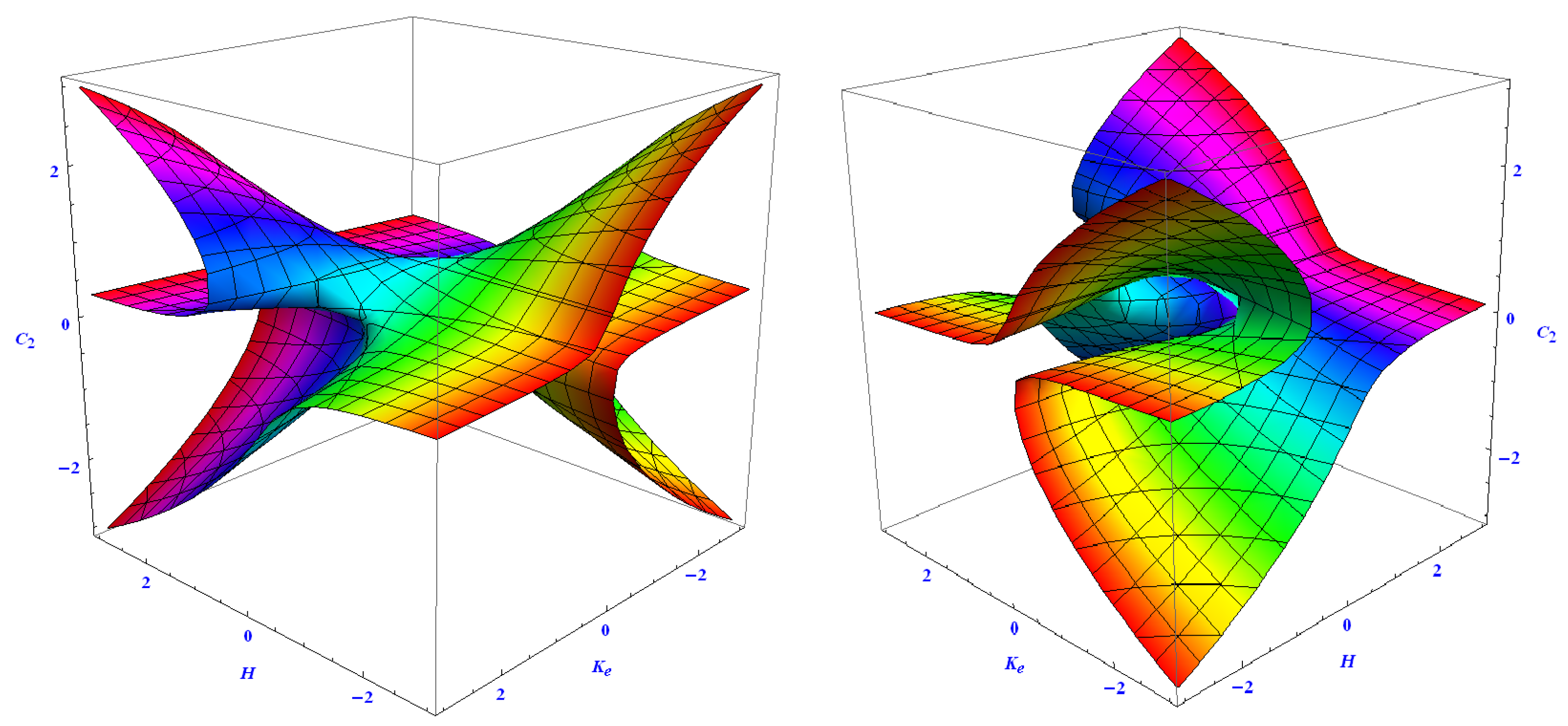
respectively. Equations (42) and (43) are the implicit algebraic surfaces. See Figure 3 and Figure 4, respectively.

Figure 3. Algebraic surface ${\mathrm{\Omega }}_1\left(H,{\mathfrak{C}}_2,K_e\right)=0$. (Left) Front view, (Right) back view.

Figure 4. Algebraic surface ${\mathrm{\Omega }}_2\left(H,{\mathfrak{C}}_2,K_e\right)=0$ in. (Left) Front side view, (Right) back side view.

$K_e$ solutions of Equations (42) and (43) and are as follows

$$\begin{array}{ccc}\hfill K_e& =& \left(18{\mathfrak{C}}_2-27H^2+2\right)H\pm (18{\mathfrak{C}}_2^3+6{\mathfrak{C}}_2^2-2{\mathfrak{C}}_2+1+81{\mathfrak{C}}_2^2{H}^2\hfill \\ & & -486{\mathfrak{C}}_2{H}^4+36{\mathfrak{C}}_2{H}^2+486H^6-81H^4+7H^2{)}^{1/2},\hfill \\ \hfill K_e& =& {\displaystyle \frac{1}{2}}\left(\left(9{\mathfrak{C}}_2-2\right)H\pm {\left({\left(9{\mathfrak{C}}_2-2\right)}^2{H}^2-4\left(9{\mathfrak{C}}_2^3-3{\mathfrak{C}}_2^2-{\mathfrak{C}}_2-1\right)\right)}^{1/2}\right),\hfill \end{array}$$

respectively.

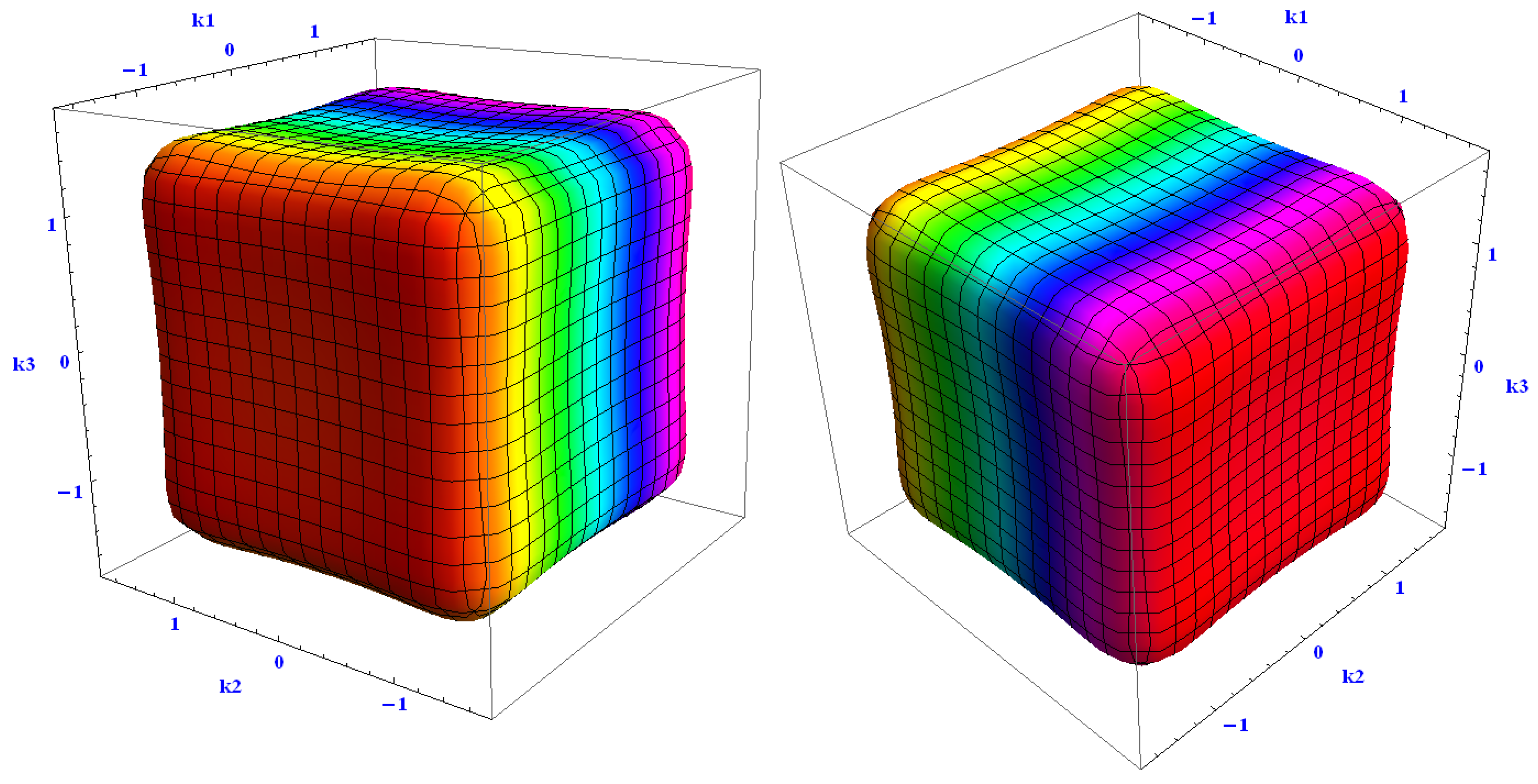
We also obtain that the implicit algebraic surfaces depend on the principal curvatures $k_1, k_2, k_3$ as ${\mathrm{\Omega }}_1\left(k_1,k_2,k_3\right)=0$ and ${\mathrm{\Omega }}_2\left(k_1,k_2,k_3\right)=0,$ replacing $H,{\mathfrak{C}}_2,K_e$ with ${\displaystyle \frac{k_1+k_2+k_3}{3}},$ ${\displaystyle \frac{k_1{k}_2+k_1{k}_3+k_2{k}_3}{3}},$ $k_1{k}_2{k}_3,$ respectively, in Equation (42) and Equation (43). See Figure 5 and Figure 6 for the algebraic surfaces ${\mathrm{\Omega }}_1, {\mathrm{\Omega }}_2,$ respectively.

Figure 5. Algebraic surface ${\mathrm{\Omega }}_1\left(k_1,k_2,k_3\right)=0$. (Left) Front side view, (Right) back side view.

Figure 6. Algebraic surface ${\mathrm{\Omega }}_2\left(k_1,k_2,k_3\right)=0$. (Left) Front side view, (Right) back side view.

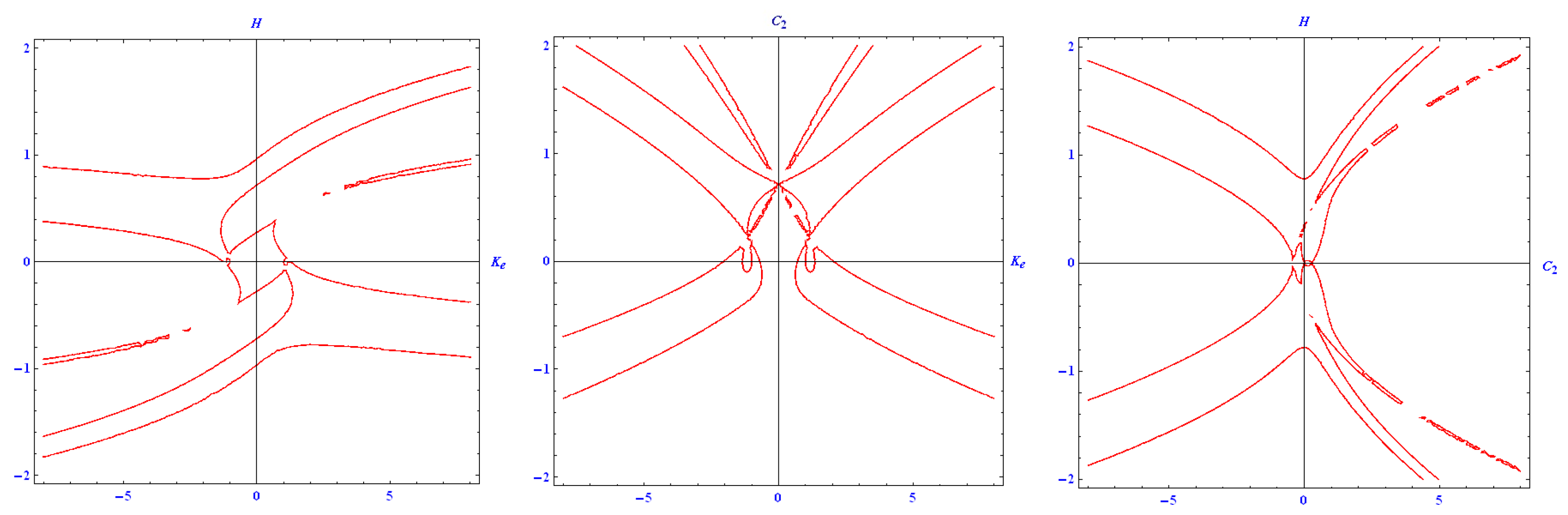
Eliminating ${\mathfrak{C}}_2,H,K_e,$ respectively, in Equation (42) and Equation (43), we have the following implicit algebraic equations. ${\mathrm{\Omega }}_3\left(H,K_e\right)=0$ (see Figure 7, Left), ${\mathrm{\Omega }}_3\left({\mathfrak{C}}_2,K_e\right)=0$ (See Figure 7, Middle), and ${\mathrm{\Omega }}_3\left(H,{\mathfrak{C}}_2\right)=0$ (see Figure 7, Right), respectively.

$$\begin{array}{ccc}\hfill {\mathrm{\Omega }}_3\left(H,K_e\right)& =& -387420489H^{18}+387420489H^{16}+516560652H^{15}{K}_e\hfill \\ & & -33480783H^{14}-420901272H^{13}{K}_e-200884698H^{12}{K}_e^2\hfill \\ & & +60584274H^{12}+74401740H^{11}{K}_e+136580337H^{10}{K}_e^2\hfill \\ & & +18068994H^9{K}_e^3-49483062H^{10}-49837356H^9{K}_e\hfill \\ & & -30114990H^8{K}_e^2-12045996H^7{K}_e^3+177147H^6{K}_e^4\hfill \\ & & +2827791H^8+15348366H^7{K}_e+8815797H^6{K}_e^2\hfill \\ & & +2033910H^5{K}_e^3+347733H^4{K}_e^4-39366H^3{K}_e^5\hfill \\ & & -1081107H^6-783918H^5{K}_e-1579014H^4{K}_e^2\hfill \\ & & -265842H^3{K}_e^3-23328H^2{K}_e^4-7290H{K}_e^5-729K_e^6\hfill \\ & & -43335H^4+278208H^3{K}_e+41292H^2{K}_e^2+17100H{K}_e^3\hfill \\ & & +2871K_e^4-10332H^2-9810H{K}_e-3699K_e^2+1557,\hfill \end{array}$$

$$\begin{array}{ccc}\hfill {\mathrm{\Omega }}_3\left({\mathfrak{C}}_2,K_e\right)& =& -387420489{\mathfrak{C}}_2^{18}+774840978{\mathfrak{C}}_2^{17}+516560652{\mathfrak{C}}_2^{15}{K}_e^2\hfill \\ & & -387420489{\mathfrak{C}}_2^{16}-903981141{\mathfrak{C}}_2^{14}{K}_e^2-200884698{\mathfrak{C}}_2^{12}{K}_e^4\hfill \\ & & +114791256{\mathfrak{C}}_2^{15}+449599086{\mathfrak{C}}_2^{13}{K}_e^2+306110016{\mathfrak{C}}_2^{11}{K}_e^4\hfill \\ & & +18068994{\mathfrak{C}}_2^9{K}_e^6-286978140{\mathfrak{C}}_2^{14}-157306536{\mathfrak{C}}_2^{12}{K}_e^2\hfill \\ & & -150929244{\mathfrak{C}}_2^{10}{K}_e^4-24446286{\mathfrak{C}}_2^8{K}_e^6+177147{\mathfrak{C}}_2^6{K}_e^8\hfill \\ & & +153055008{\mathfrak{C}}_2^{13}+199113228{\mathfrak{C}}_2^{11}{K}_e^2+39090438{\mathfrak{C}}_2^9{K}_e^4\hfill \\ & & +10628820{\mathfrak{C}}_2^7{K}_e^6-39366{\mathfrak{C}}_2^3{K}_e^{10}+2125764{\mathfrak{C}}_2^{12}\hfill \\ & & -99615663{\mathfrak{C}}_2^{10}{K}_e^2-24229773{\mathfrak{C}}_2^8{K}_e^4+2342277{\mathfrak{C}}_2^6{K}_e^6\hfill \\ & & -91854{\mathfrak{C}}_2^4{K}_e^8+45927{\mathfrak{C}}_2^2{K}_e^{10}-729K_e^{12}+46766808{\mathfrak{C}}_2^{11}\hfill \\ & & +17990262{\mathfrak{C}}_2^9{K}_e^2+14464818{\mathfrak{C}}_2^7{K}_e^4-4531464{\mathfrak{C}}_2^5{K}_e^6\hfill \\ & & +77274{\mathfrak{C}}_2^3{K}_e^8-10206{\mathfrak{C}}_2{K}_e^{10}-25863462{\mathfrak{C}}_2^{10}\hfill \\ & & -13161366{\mathfrak{C}}_2^8{K}_e^2-2138886{\mathfrak{C}}_2^6{K}_e^4+1972188{\mathfrak{C}}_2^4{K}_e^6\hfill \\ & & -125145{\mathfrak{C}}_2^2{K}_e^8+5994K_e^{10}-5117580{\mathfrak{C}}_2^9+7619508{\mathfrak{C}}_2^7{K}_e^2\hfill \\ & & -57834{\mathfrak{C}}_2^5{K}_e^4-259686{\mathfrak{C}}_2^3{K}_e^6+19818{\mathfrak{C}}_2{K}_e^8-5078214{\mathfrak{C}}_2^8\hfill \\ & & -1570995{\mathfrak{C}}_2^6{K}_e^2-141426{\mathfrak{C}}_2^4{K}_e^4+106146{\mathfrak{C}}_2^2{K}_e^6-16551K_e^8\hfill \\ & & +2152008{\mathfrak{C}}_2^7-303750{\mathfrak{C}}_2^5{K}_e^2-2970{\mathfrak{C}}_2^3{K}_e^4+18396{\mathfrak{C}}_2{K}_e^6\hfill \\ & & +819396{\mathfrak{C}}_2^6-326268{\mathfrak{C}}_2^4{K}_e^2-76158{\mathfrak{C}}_2^2{K}_e^4+20700K_e^6\hfill \\ & & +454896{\mathfrak{C}}_2^5+97524{\mathfrak{C}}_2^3{K}_e^2-49716{\mathfrak{C}}_2{K}_e^4-43740{\mathfrak{C}}_2^4\hfill \\ & & +80919{\mathfrak{C}}_2^2{K}_e^2-13383K_e^4-40824{\mathfrak{C}}_2^3+26082{\mathfrak{C}}_2{K}_e^2\hfill \\ & & -24057{\mathfrak{C}}_2^2+4698K_e^2-4374{\mathfrak{C}}_2-729,\hfill \end{array}$$

$$\begin{array}{ccc}\hfill {\mathrm{\Omega }}_3\left(H,{\mathfrak{C}}_2\right)& =& 4782969H^{12}-9565938{\mathfrak{C}}_2{H}^{10}+4782969{\mathfrak{C}}_2^2{H}^8\hfill \\ & & -3188646H^{10}+1062882{\mathfrak{C}}_2^3{H}^6+6731586{\mathfrak{C}}_2{H}^8\hfill \\ & & -1062882{\mathfrak{C}}_2^4{H}^4-4901067{\mathfrak{C}}_2^2{H}^6+413343H^8\hfill \\ & & +1417176{\mathfrak{C}}_2^3{H}^4-944784{\mathfrak{C}}_2{H}^6+59049{\mathfrak{C}}_2^6\hfill \\ & & -157464{\mathfrak{C}}_2^4{H}^2+597051{\mathfrak{C}}_2^2{H}^4-223074H^6\hfill \\ & & +13122{\mathfrak{C}}_2^5-83106{\mathfrak{C}}_2^3{H}^2+266814{\mathfrak{C}}_2{H}^4\hfill \\ & & -12393{\mathfrak{C}}_2^4-78003{\mathfrak{C}}_2^2{H}^2+50301H^4-1458{\mathfrak{C}}_2^3\hfill \\ & & -27702{\mathfrak{C}}_2{H}^2+729{\mathfrak{C}}_2^2-2916H^2.\hfill \end{array}$$

Figure 7. Algebraic curves. (Left) ${\mathrm{\Omega }}_3\left(H,K_e\right)=0,$ (Middle) ${\mathrm{\Omega }}_3\left({\mathfrak{C}}_2,K_e\right)=0$, and (Right) ${\mathrm{\Omega }}_3\left(H,{\mathfrak{C}}_2\right)=0$.

We obtain the implicit algebraic surface, which depends on principal curvatures $k_1, k_2, k_3$ as ${\mathrm{\Omega }}_3\left(k_1,k_2,k_3\right)=0,$ replacing $H,K_e$ with ${\displaystyle \frac{k_1+k_2+k_3}{3}},$ $k_1{k}_2{k}_3,$ respectively, in ${\mathrm{\Omega }}_3\left(H,K_e\right)=0.$ See Figure 8 for the algebraic surface ${\mathrm{\Omega }}_3$.

Figure 8. Algebraic surface ${\mathrm{\Omega }}_3\left(k_1,k_2,k_3\right)=0$. (Left) Front side view, (Right) back side view.

3.2. Second Solution of the Pythagorean Quadruple Formula ${\mathcal{P}}_4$

Before defining the umbilical hypersurface in 4-space, we make some remarks.

Remark 1.

The following are equivalent

$$\begin{array}{ccc}{k}_1=k_2=k_3& \iff & k_1-k_2=0\wedge k_1-k_3=0\wedge k_2-k_3=0\\ & \iff & {\left(k_1-k_2\right)}^2=0\wedge {\left(k_1-k_3\right)}^2=0\wedge {\left(k_2-k_3\right)}^2=0\\ & \iff & \left\{\begin{array}{c}{k}_1^2-2k_1{k}_2+k_2^2=0\\ k_1^2-2k_1{k}_3+k_3^2=0\\ k_2^2-2k_2{k}_3+k_3^2=0\end{array}\right\}\\ & \iff & k_1^2+k_2^2+k_3^2=k_1{k}_2+k_1{k}_3+k_2{k}_3(\mathit{Adding}\mathit{above}\mathit{eqs}.)\\ & \iff & H^2={\mathfrak{C}}_2.\end{array}$$

Remark 2.

The following are equivalent

$$\begin{array}{ccc}{k}_1=k_2=k_3& \iff & k_1-k_2=0\wedge k_1-k_3=0\wedge k_2-k_3=0\\ & \iff & {\left(k_1-k_2\right)}^2=0\wedge {\left(k_1-k_3\right)}^2=0\wedge {\left(k_2-k_3\right)}^2=0\\ & \iff & \left\{\begin{array}{c}{k}_1^2+2k_1{k}_2+k_2^2=4k_1{k}_2\\ k_1^2+2k_1{k}_3+k_3^2=4k_1{k}_3\\ k_2^2+2k_2{k}_3+k_3^2=4k_2{k}_3\end{array}\right\}\\ & \iff & {\left(k_1+k_2\right)}^2=4k_1{k}_2\wedge {\left(k_1+k_3\right)}^2=4k_1{k}_3\wedge {\left(k_2+k_3\right)}^2=4k_2{k}_3\\ & \iff & \left(k_1+k_2\right)\left(k_1+k_3\right)\left(k_2+k_3\right)=8k_1{k}_2{k}_3\\ & \iff & H{\mathfrak{C}}_2=K_e.\end{array}$$

Remark 3.

Using the results of the Remarks 1 and 2 together, we have

$$k_1=k_2=k_3\iff H^3=K_e.$$

Next, we describe the umbilical hypersurface of four dimensional space.

Definition 2.

The hypersurface $M^3$ immersed into a ${\mathbb{M}}^4\left(\mathbf{c}\right)$, $\mathbf{c}\in \{-1,0,1\}$ is called umbilical if all its points are umbilical, i.e., $k_1=k_2=k_3$ or, equivalently, $H^3-K_e=0,$ with $H{\mathfrak{C}}_2=K_e,$$H^2={\mathfrak{C}}_2$.

The only umbilical hypersurfaces are (open to) hyperplanes and hyperspheres in ${\mathbb{M}}^4\left(\mathbf{c}\right)$.

Next, taking determinants of both sides of

$$\left(\begin{array}{ccc}{\mathcal{Y}}_{11}& {\mathcal{Y}}_{12}& {\mathcal{Y}}_{13}\\ {\mathcal{Y}}_{12}& {\mathcal{Y}}_{22}& {\mathcal{Y}}_{23}\\ {\mathcal{Y}}_{13}& {\mathcal{Y}}_{23}& {\mathcal{Y}}_{33}\end{array}\right)=\left(\begin{array}{ccc}0& 0& 0\\ 0& 0& 0\\ 0& 0& 0\end{array}\right),$$

(44)

we obtain

$$\begin{array}{ccc}\hfill 0& =& -[\left(k_1^2{k}_2^4+k_1^4{k}_2^2+k_1^2{k}_3^4+k_1^4{k}_3^2+k_2^2{k}_3^4+k_2^4{k}_3^2\right)\hfill \\ & & +6k_1^2{k}_2^2{k}_3^2+2\left(k_1^3{k}_2^3+k_1^3{k}_3^3+k_2^3{k}_3^3\right)+2k_1{k}_2{k}_3\left(k_1^3+k_2^3+k_3^3\right)\hfill \\ & & -2k_1{k}_2{k}_3\left(k_1{k}_2^2+k_1^2{k}_2+k_1{k}_3^2+k_1^2{k}_3+k_2{k}_3^2+k_2^2{k}_3\right)]\left(K_e^2+M^2+T^2-1\right).\hfill \end{array}$$

Here, ${\mathcal{Y}}_{ij}$ are given by Equations (34), (35), (36), (37), (38), and (39), respectively. Hence, the above Equation reduces to

$$-{\left(k_1-k_2\right)}^2{\left(k_1-k_3\right)}^2{\left(k_2-k_3\right)}^2\left(K_e^2+M^2+T^2-1\right)=0.$$

(45)

Then, $-{\left(k_1-k_2\right)}^2{\left(k_1-k_3\right)}^2{\left(k_2-k_3\right)}^2$ transforms to the following

$$-{\left(k_2-k_3\right)}^2{\left(k_1-k_3\right)}^2{\left(k_1-k_2\right)}^2=27\left(4H^3{K}_e-3{\mathfrak{C}}_2^2{H}^2+4{\mathfrak{C}}_2^3+K_e^2-6{\mathfrak{C}}_{2}H{K}_e\right),$$

by using

$$\begin{array}{ccc}\hfill k_1^2{k}_2^4+k_1^4{k}_2^2+k_1^2{k}_3^4+k_1^4{k}_3^2+k_2^2{k}_3^4+k_2^4{k}_3^2& =& \left(T^2-2M{K}_e\right)\left(M^2-2T\right)-3K_e^2\hfill \\ & =& \left(9{\mathfrak{C}}_2^2-6H{K}_e\right)\left(9H^2-6{\mathfrak{C}}_2\right)-3K_e^2.\hfill \end{array}$$

Therefore, we obtain the following.

Corollary 4.

Since $H^2={\mathfrak{C}}_2,$ $H{\mathfrak{C}}_2=K_e,$ $H^3=K_e$, the determinant of the ${\mathcal{P}}_4$ matrix (44) satisfies

$$4H^3{K}_e-3{\mathfrak{C}}_2^2{H}^2+4{\mathfrak{C}}_2^3+K_e^2-6{\mathfrak{C}}_{2}H{K}_e=0,$$

by using

$$\begin{array}{ccc}\hfill k_1^3{k}_2^3+k_1^3{k}_3^3+k_2^3{k}_3^3& =& T^3-3TM{K}_e+3K_e^2\hfill \\ & =& 27{\mathfrak{C}}_2^3-27H{\mathfrak{C}}_2{K}_e+3K_e^2.\hfill \end{array}$$

We also have the following.

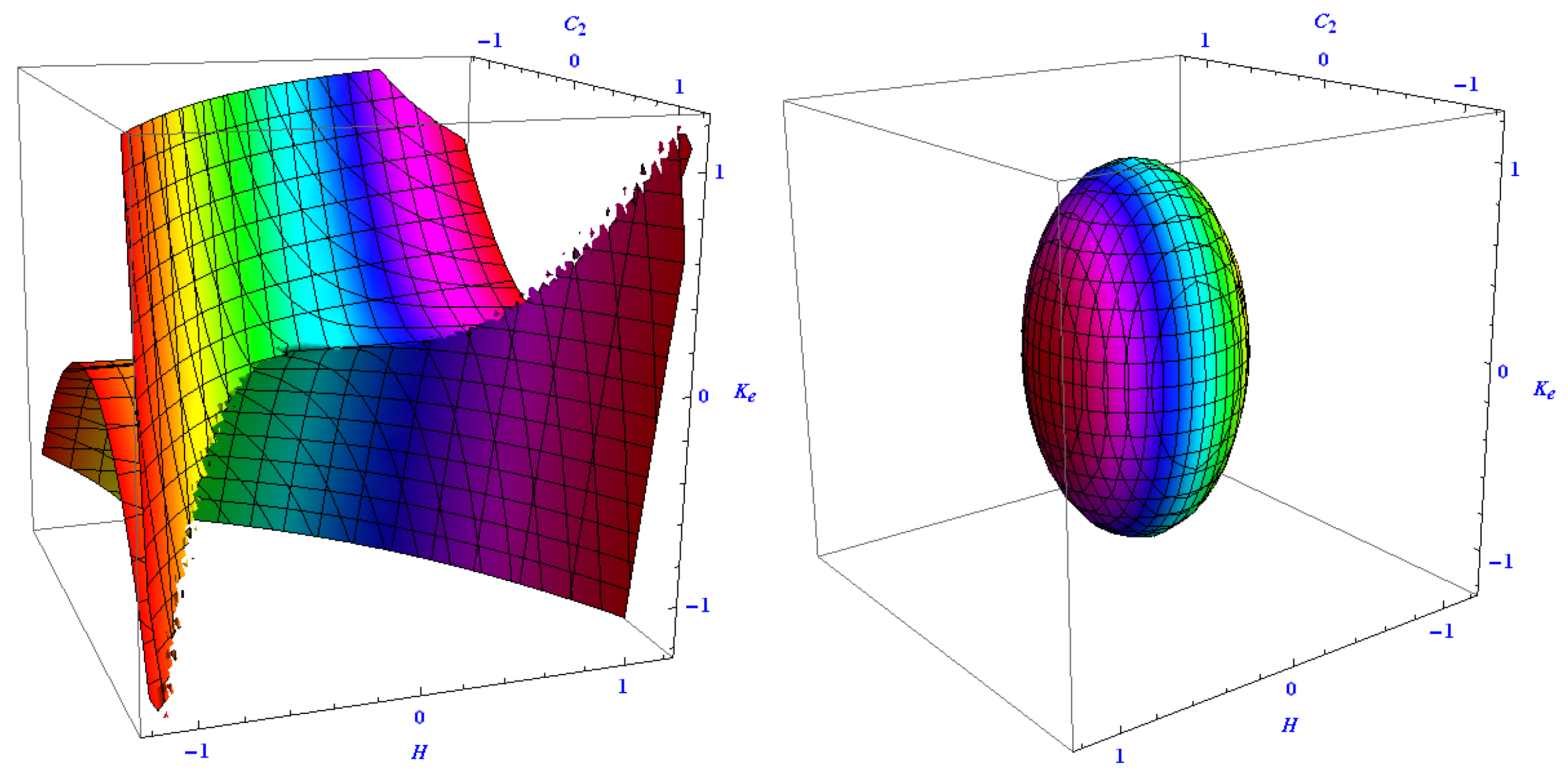
Corollary 5 (Geometric Conclusion 2).

The determinant given by Equation (45) of the ${\mathcal{P}}_4$ matrix described by Equation (44) draws the surface $K_e=H^3$ with $H^2={\mathfrak{C}}_2,$ $H{\mathfrak{C}}_2=K_e$ and the ellipsoid surface ${\left(3H\right)}^2+{\left(3{\mathfrak{C}}_2\right)}^2+K_e^2=1.$

The determinant of the ${\mathcal{P}}_4$ is also given by as follows

$$27\left(4H^3{K}_e-3{\mathfrak{C}}_2^2{H}^2+4{\mathfrak{C}}_2^3+K_e^2-6{\mathfrak{C}}_{2}H{K}_e\right)\left({\left(3H\right)}^2+{\left(3{\mathfrak{C}}_2\right)}^2+K_e^2-1\right)=0.$$

Here, $4H^3{K}_e-3{\mathfrak{C}}_2^2{H}^2+4{\mathfrak{C}}_2^3+K_e^2-6{\mathfrak{C}}_{2}H{K}_e=0$ is the implicit surface as ${\mathrm{\Theta }}_1\left(H,{\mathfrak{C}}_2,K_e\right)=0$ (See Figure 9, Left), satisfying $H^3-K_e=0,$ with $H{\mathfrak{C}}_2=K_e,$$H^2={\mathfrak{C}}_2$, and the implicit ellipsoid, or ellipsoidal surface ${\left(3H\right)}^2+{\left(3{\mathfrak{C}}_2\right)}^2+K_e^2=1$ as ${\mathrm{\Theta }}_2\left(H,{\mathfrak{C}}_2,K_e\right)=0$ (See Figure 9, Right).

Figure 9. Algebraic surfaces. (Left) ${\mathrm{\Theta }}_1\left(H,{\mathfrak{C}}_2,K_e\right)=0$, (Right) ${\mathrm{\Theta }}_2\left(H,{\mathfrak{C}}_2,K_e\right)=0$.

Hence, extending the determinant of the ${\mathcal{P}}_4,$ we obtain the implicit algebraic surface $\mathrm{\Psi }\left(H,{\mathfrak{C}}_2,K_e\right)=0,$ as follows (see Figure 10):

$$\begin{array}{ccc}\hfill \mathrm{\Psi }\left(H,{\mathfrak{C}}_2,K_e\right)& =& -108H^3{K}_e+972H^5{K}_e+81{\mathfrak{C}}_2^2{H}^2+972{\mathfrak{C}}_2^3{H}^2-729{\mathfrak{C}}_2^2{H}^4\hfill \\ & & -729{\mathfrak{C}}_2^4{H}^2+243{\mathfrak{C}}_2^2{K}_e^2+108{\mathfrak{C}}_2^3{K}_e^2+243H^2{K}_e^2+108H^3{K}_e^3\hfill \\ & & -108{\mathfrak{C}}_2^3+972{\mathfrak{C}}_2^5-27K_e^2+27K_e^4-81{\mathfrak{C}}_2^2{H}^2{K}_e^2-162{\mathfrak{C}}_{2}H{K}_e^3\hfill \\ & & -1458{\mathfrak{C}}_2{H}^3{K}_e-1458{\mathfrak{C}}_2^{3}H{K}_e+972{\mathfrak{C}}_2^2{H}^3{K}_e+162{\mathfrak{C}}_{2}H{K}_e.\hfill \end{array}$$

Figure 10. Algebraic surface $\mathrm{\Psi }\left(H,{\mathfrak{C}}_2,K_e\right)=0$. (Left) Front side view, (Right) back side view.

Corollary 6.

The determinant given by Equation (45) of the ${\mathcal{P}}_4$ matrix described by Equation (44) corresponds to an umbilical round hypersphere where the principal curvatures satisfy $k_1=k_2=k_3$. In other words, it satisfies $H^3=K_e$ with $H{\mathfrak{C}}_2=K_e$ and $H^2={\mathfrak{C}}_2$ in ${\mathbb{M}}^4\left(\mathbf{c}\right)$, where $\mathbf{c}\in \{-1,0,1\}$.

We remark that this work relies on the Phythagorean formula but does not depend on the distance between points in the running space form.

On the other hand, we use the upper hypersphere ${\mathbb{S}}^3\left(r\right)$ with the Cartesian map $\mathbf{x}:$${\mathbb{E}}^3\to {\mathbb{S}}^3\left(r\right)\subset {\mathbb{E}}^4$ given by

$$\left(u,v,w\right)\mapsto \left(u,v,w,\sqrt{r^2-u^2-v^2-w^2}\right),$$

(46)

where $r>0.$ Next, we compute the fundamental forms of the upper hypersphere given by Equation (46). The first fundamental form matrix of it as follows

$$I=\left(\begin{array}{ccc}{\displaystyle \frac{r^2-v^2-w^2}{r^2-u^2-v^2-w^2}}& {\displaystyle \frac{uv}{r^2-u^2-v^2-w^2}}& {\displaystyle \frac{uw}{r^2-u^2-v^2-w^2}}\\ {\displaystyle \frac{uv}{r^2-u^2-v^2-w^2}}& {\displaystyle \frac{r^2-u^2-w^2}{r^2-u^2-v^2-w^2}}& {\displaystyle \frac{vw}{r^2-u^2-v^2-w^2}}\\ {\displaystyle \frac{uw}{r^2-u^2-v^2-w^2}}& {\displaystyle \frac{vw}{r^2-u^2-v^2-w^2}}& {\displaystyle \frac{r^2-u^2-v^2}{r^2-u^2-v^2-w^2}}\end{array}\right),$$

Then, the shape operator matrix is given by $\mathbf{S}={\displaystyle \frac{1}{r}}{\mathcal{I}}_3.$ We obtain $II=I.\mathbf{S},$ $III=II.\mathbf{S}$, and $IV=III.\mathbf{S},$ easily.

Taking into account the Pythagorean quadruple formula $\underset{\mathrm{\Omega }}{\underbrace{I^2+I{I}^2+II{I}^2}}=\underset{\mathrm{\Phi }}{\underbrace{I{V}^2}},$ of the hypersphere described by Equation (46), and considering $det\left(\mathrm{\Omega }\right)=det\left(\mathrm{\Phi }\right),$ we have the following.

Corollary 7.

The hypersphere given by Equation (46) has the Pythagorean quadruple formula mentioned by (29) if and only if the following holds

$$r^6\left(r^{12}+3r^{10}+6r^8+7r^6+6r^4+3r^2+1\right)-1=0.$$

The roots of above equation are $r_1=-0.73735\in {\mathbb{R}}^{-},$ $r_2=0.73735\in {\mathbb{R}}^{+}, r_{3,4,\dots ,18}\in \mathbb{C}.$ Here, the positive and real $r_2$ solution is also given in the second row of the Table 1.

Table 1. x and r solutions of Pythagorean 3–26-tuples.

Dimension	x (11 Digits)	r (11 Digits)
3	$0.6180349887$	$0.7861513777$
4	$0.5436890126$	$0.7373527058$
5	$0.5187900636$	$0.7202708266$
6	$0.5086603916$	$0.7132043127$
7	$0.5041382583$	$0.7100269420$
8	$0.5020170551$	$0.7085316191$
9	$0.5009941779$	$0.7078094220$
10	$0.5004931182$	$0.7074553826$
11	$0.5002454622$	$0.7072803279$
12	$0.5001224294$	$0.7071933466$
13	$0.5000611322$	$0.7071500069$
14	$0.5000305436$	$0.7071283785$
15	$0.5000152657$	$0.7071175757$
16	$0.5000076312$	$0.7071121773$
17	$0.5000038151$	$0.7071094789$
18	$0.5000019074$	$0.7071081300$
19	$0.5000009537$	$0.7071074556$
20	$0.5000004768$	$0.7071071183$
21	$0.5000002384$	$0.7071069498$
22	$0.5000001192$	$0.7071068655$
23	$0.5000000596$	$0.7071068233$
24	$0.5000000298$	$0.7071068023$
25	$0.5000000149$	$0.7071067917$
26	$0.5000000074$	$0.7071067864$

Let $M^3$ be an immersed hypersurface into ${\mathbb{H}}^4$, ${\mathbb{E}}^4$, or ${\mathbb{S}}^4.$$M^3$ is named totally geodesic while $II=0$ and totally umbilical while $II=\mu I$, where $\mu \ne 0$ is a constant. When $II=0$, then $III=0$ and $IV=0$. This is not possible for the Pythagorean ${\mathcal{P}}_4$ formula. On the other hand, while $II$ is degenerate (i.e., $det\left(II\right)=0$), using Equations (28) and (29), and considering $III=II.\mathbf{S}=I.{\mathbf{S}}^2,$ $K_e=det\mathbf{S},$ we obtain $I=0$, which contradicts $det\left(II\right)=0.$ So, $det\left(II\right)\ne 0.$

When $M^3$ is minimal, and $K_e\ne 0,$ using Equations (28) and (29) again, we find the following:

$$\left(K_e^2-1\right)I^2=\left(1-{\left(3{\mathfrak{C}}_2\right)}^2\right)I{I}^2.$$

Taking both sides of the determinant, we have

$$K_e^6-3K_e^4+\left({\left(3{\mathfrak{C}}_2\right)}^2+2\right)K_e^2-1=0.$$

(47)

Here, $K_e$ has 4 complex roots, 1 negative real root ($K_e=-1.3936$, ${\mathfrak{C}}_2=-0.251538$), and the following positive real root ($K_e=0.317103,$${\mathfrak{C}}_2=0.956641)$

$$K_e={\left(0.381571c-{\displaystyle \frac{7.86222{\left({\mathfrak{C}}_2\right)}^2}{c}}+{\displaystyle \frac{0.87358}{c}}+1\right)}^{1/2},$$

where

$$c={\left(-81{\left({\mathfrak{C}}_2\right)}^2+1.73205{\left(2916{\left({\mathfrak{C}}_2\right)}^6+1215{\left({\mathfrak{C}}_2\right)}^4-378{\left({\mathfrak{C}}_2\right)}^2+23\right)}^{1/2}+9\right)}^{1/3}.$$

Then, $K_e$ is a constant. When the space is ${\mathbb{H}}^4$ or ${\mathbb{E}}^4$, then $M^3$ should be totally geodesic (see [23,24] for $M^2$ case.). Then, it gives a contradiction.

Therefore, the case of $K_e=1$ and $M^3$ is totally geodesic and does not take place. The case of $K_e=0$, $M^3$ is an open piece of the Clifford torus. Then, $K_e=-1$, which is incompatible with Equation (47). So, the immersed hypersurface into ${\mathbb{H}}^4$, ${\mathbb{E}}^4$, or ${\mathbb{S}}_{+}^4$ supplying the ${\mathcal{P}}_4$ formula mentioned by Equation (29) cannot be totally geodesic, may not be minimal, and does not have a degenerate second fundamental form.

On the other side, we want to see the real solutions of ${\displaystyle \sum _{k=1}^n}{x}^k-1=0$ for some integers. See Table 1, Table 2, Table 3 and Table 4 for some solutions to it. To see the real solutions of ${\displaystyle \sum _{k=1}^{99999}}{x}^k-1=0$ in ${\mathbb{E}}^{100000}$ on graphics depending on x and r, respectively, see Figure 11.

Table 2. x and r solutions of Pythagorean $30,40,50$-tuples.

Dimension	x (17 Digits)	r (17 Digits)
30	$0.5000000004656613$	$0.7071067815158197$
40	$0.5000000000004547$	$0.7071067811868691$
50	$0.5000000000000004$	$0.7071067811865478$

Table 3. x and r solutions of Pythagorean 75-tuples of ${\mathbb{S}}^{74}\left(r\right)$ in ${\mathbb{E}}^{75}$.

Dimension	75
x (27 digits)	$0.50000000000000000000001323$
r (27 digits)	$0.70710678118654752440085372$

Table 4. x and r solutions of Pythagorean 100-tuples of ${\mathbb{S}}^{99}\left(r\right)$ in ${\mathbb{E}}^{100}$.

Dimension	100
x (41 digits)	$0.5000000000000000000000000000003944304526$
r (41 digits)	$0.7071067811865475244008443621051279437326$

Figure 11. Real graphics of the Pythagorean ${10}^5$-tuples of ${\mathbb{S}}^{99999}\left(r\right)$. (Left) $y={\displaystyle \sum _{k=1}^{99999}}{x}^k-1,$$x\approx {\displaystyle \frac{1}{2}},($Right$)y={\displaystyle \sum _{k=1}^{99999}}{r}^{2k}-1,$$r\approx {\displaystyle \frac{1}{\sqrt{2}}}$.

In dimension 200, i.e., in ${\mathbb{E}}^{200}$, x and r solutions of the Pythagorean 200-tuples of the ${\mathbb{S}}^{199}\left(r\right)$ are as follows (with 321 digits):

$$\begin{array}{ccc}& & x\approx 0.5000000000000000000000000000000000000000000000000000000000003\hfill \\ & & 11150763893057085357203202689006212029512608436058356655094556658\hfill \\ & & 63343488449735236553010467476138303976881738641100895335924232023\hfill \\ & & 34114463199807863070347568289193325695011780175081122039993867410\hfill \\ & & 2867738110784051939243798551104507095592401999618923621906567756,\hfill \end{array}$$

and

$$\begin{array}{ccc}& & r\approx 0.7071067811865475244008443621051279437325833055886006739067917\hfill \\ & & 94344757197397837300988207418918995590004395380321440946772513382\hfill \\ & & 49838886753552692449588190583402000578194741957214813556875759537\hfill \\ & & 82813770690555701346636538769813156446384560892821446168091144026\hfill \\ & & 0791134133607458928495481181021022394644625344379042586920744364.\hfill \end{array}$$

Interestingly, when the dimension n increasing regularly, we observe that $x\to {\displaystyle \frac{1}{2}},$ and $r\to {\displaystyle \frac{1}{\sqrt{2}}}$ from all of the above results. To understand the larger results of the Pythagorean ${10}^5$-tuples, virtually, see Figure 11.

4. Pythagorean $\left(n+1\right)$-Tuples ${\mathcal{P}}_{n+1}$

In this section, considering all findings of the previous two sections, we obtain the generalized Pythagorean formula ${\mathcal{P}}_{n+1},$ using the fundamental form matrices for the hypersurfaces in higher dimension space forms.

Theorem 2.

Let a hypersurface $M^n$ immersed into a $(n+1)$-dimensional Riemannian space form ${\mathbb{M}}^{n+1}\left(\mathbf{c}\right)$, $\mathbf{c}\in \{-1,0,1\}$ satisfy the following Pythagorean $\left(n+1\right)$-tuples ${\mathcal{P}}_{n+1}$ equation

$$I^2+I{I}^2+II{I}^2+\dots +N^2={(N+1)}^2,$$

(48)

if and only if the following algebraic equation holds:

$$\sum _{k=1}^n{x}^k-1=0,$$

where $x=r^2.$ Here, $I,II,III,\cdots ,N,N+1$ are the fundamental form matrices of the hypersurface $M^n$.

Proof. 

Let $M^n$ be an immersed hypersurface into ${\mathbb{H}}^{n+1}$, ${\mathbb{E}}^{n+1}$, or ${\mathbb{S}}^{n+1}.$ The shape operator matrix is given by $\mathbf{S}={\displaystyle \frac{1}{r}}{\mathcal{I}}_n,$ where ${\mathcal{I}}_n$ is the identitity matrix. The ${\mathcal{P}}_{n+1}$ given by Equation (48) of the hypersurface can be denoted by

$${\left({\mathcal{I}}_n\right)}^2+{\left(\mathbf{S}\right)}^2+{\left({\mathbf{S}}^2\right)}^2+\dots +{\left({\mathbf{S}}^{n-1}\right)}^2={\left({\mathbf{S}}^n\right)}^2.$$

Considering the ${\mathcal{P}}_{n+1}$ determined by Equation (48) with the fundamantel form matrices of the hypersurface, we obtain $r^{2n}+r^{2n-2}+\dots +r^2-1=0,$ and $r\ne 0.$ The hypersurface $M^n$ has the Pythagorean $\left(n+1\right)$-tuples ${\mathcal{P}}_{n+1}$ described by Equation if and only if algebraic equation $x^n+x^{n-1}+\dots +x-1=0$ holds, where $x=r^2$.

Additionally, the geometric series is defined by ${\displaystyle \sum _{k=0}^{\infty }}{x}^k={\displaystyle \frac{1}{1-x}},$ where $\left|x\right|<1$. Therefore, we have the following

$$\begin{array}{ccc}{\displaystyle \sum _{k=1}^{\infty }}{x}^k-1=0\hfill & \iff \hfill & {\displaystyle \sum _{k=0}^{\infty }}{x}^k-2=0\hfill \\ \hfill & \hfill & \\ \hfill & \iff \hfill & {\displaystyle \frac{-1+2x}{1-x}}=0,x\ne 1\hfill \\ \hfill & \hfill & \\ \hfill & \iff \hfill & x={\displaystyle \frac{1}{2}}\hfill \\ \hfill & \hfill & \\ \hfill & \iff \hfill & r={\displaystyle \frac{1}{\sqrt{2}}},\left(x=r^2,r>0\right).\hfill \end{array}$$

(49)

□

Corollary 8.

Let $M^n$ be an immersed hypersphere into ${\mathbb{M}}^{n+1}\left(\mathbf{c}\right)$, $\mathbf{c}\in \{-1,0,1\}$ with radius r satisfying the Pythagorean $\left(n+1\right)$-tuples ${\mathcal{P}}_{n+1}$ mentioned by Equation (48). When $n\to \infty ,$ then $N\to \infty ,$ and $r\to {\displaystyle \frac{1}{\sqrt{2}}}$.

Next, we define the umbilic hypersurface, then give a generalization of the determinant of the Pythagorean $\left(n+1\right)$-tuples ${\mathcal{P}}_{n+1}$ formula.

Definition 3.

The hypersurface $M^n$ immersed into a $(n+1)$-dimensional Riemannian space form ${\mathbb{M}}^{n+1}\left(\mathbf{c}\right)$, $\mathbf{c}\in \{-1,0,1\}$ is called umbilical if all its points are umbilical, i.e., $k_1=k_2=\dots =k_n,$ or, equivalently, $H^n-K_e=0$.

Proposition 1.

Let a hypersurface $M^n$ immersed into a ${\mathbb{M}}^{n+1}\left(\mathbf{c}\right)$, $\mathbf{c}\in \{-1,0,1\}$ satisfy the Pythagorean $\left(n+1\right)$-tuples ${\mathcal{P}}_{n+1}$ formula

$$I^2+I{I}^2+II{I}^2+\dots +N^2={\left(\sum _{i=1}^n{\left(-1\right)}^{i+1}\left({\displaystyle \genfrac{}{}{0pt}{}{n}{i}}\right){\mathfrak{C}}_{i}I\left({\mathbf{S}}^{n-i}\left(X\right),Y\right)\right)}^2.$$

(50)

Then, the determinant of Equation (50) is given by

$$n^n\left({\mathfrak{C}}_n-{\mathfrak{C}}_1^n\right)\left({\left(n{\mathfrak{C}}_1\right)}^2+{\left(n{\mathfrak{C}}_2\right)}^2+\dots +{\left(n{\mathfrak{C}}_{n-1}\right)}^2+{\mathfrak{C}}_n^2-1\right)=0,$$

(51)

or equivalently by

$$-\prod _{1\le i<j\le n}^n{\left(k_i-k_j\right)}^2\left(\sum _{\ell =1}^{n-1}{\left(n{\mathfrak{C}}_{\ell }\right)}^2+{\mathfrak{C}}_n^2-1\right)=0,$$

(52)

where ${\mathfrak{C}}_1=H,$${\mathfrak{C}}_n=K_e.$

Finally, we have the following.

Conjecture 1.

The determinant of the ${\mathcal{P}}_{n+1}$ matrix, as defined in Equation (50), generates a hypersurface $H^n=K_e$ and a hyperellipsoid ${\left(nH\right)}^2+{\left(n{\mathfrak{C}}_2\right)}^2+{\left(n{\mathfrak{C}}_3\right)}^2+\dots +{\left(n{\mathfrak{C}}_{n-1}\right)}^2+K_e^2=1$ in ${\mathbb{M}}^{n+1}\left(\mathbf{c}\right)$, where $\mathbf{c}\in \{-1,0,1\}$.

Then, we present the following generalization for the determinant of ${\mathcal{P}}_{n+1}$.

Conjecture 2.

The determinant given by Equation (51) (or equivalently by Equation (52)) of the ${\mathcal{P}}_{n+1}$ formula mentioned by Equation corresponds to an umbilical round hypersphere satisfying $k_1=k_2=\dots =k_n$, i.e., $H^n=K_e$, in ${\mathbb{M}}^{n+1}\left(\mathbf{c}\right)$, where $\mathbf{c}\in \{-1,0,1\}$.

5. Conclusions

This article provides a thorough investigation of the Pythagorean theorem from the perspective of differential geometry, offering insightful generalizations in higher-dimensional space forms. It establishes a connection between classical geometric identities and the intrinsic properties of hypersurfaces, filling a notable gap in the field.

Specifically, the paper generalizes that an immersed hypersphere $M^n$ with radius r in ${\mathbb{M}}^{n+1}\left(\mathbf{c}\right)$, where $\mathbf{c}\in \{-1,0,1\}$, satisfies the $(n+1)$-tuple Pythagorean formula. Furthermore, as the dimension $n\to \infty$ and the fundamental form $N\to \infty$, it is shown that $r\to {\displaystyle \frac{1}{\sqrt{2}}}$.

Finally, the paper proposes that the determinant of the Pythagorean formula characterizes an umbilical round hypersphere with equal principal curvatures, satisfying $H^n=K_e$ in ${\mathbb{M}}^{n+1}\left(\mathbf{c}\right)$. These findings contribute to a broader understanding of curvature relations and their role in the geometry of hypersurfaces.