Distributions of Outputs Given Subsets of Inputs and Dependent Generalized Sensitivity Indices

Abstract

Better understanding mathematical and numerical models often requires investigating the impacts of inputs on the model outputs, as well as interactions. Quantifying such effects for models with non-independent input variables (NIVs) relies on conditional distributions of the outputs given every subset of inputs. In this paper, by firstly providing additional dependency models of NIVs, functional outputs are composed by dependency models (yielding equivalent representations of outputs) to derive distributions of outputs conditional on inputs. We then provide an algorithm for selecting the necessary and sufficient equivalent representations that allow for obtaining all the conditional distributions of outputs given every subset of inputs, and for assessing the main, total, and interaction effects (i.e., indices) of every subset of NIVs. Unbiased estimators of covariances of sensitivity functionals and consistent estimators of such indices are derived by distinguishing the case of the multivariate and/or functional outputs, including dynamic models. Finally, analytical results and numerical results are provided, including an illustration based on a dynamic model.

1. Introduction

Mathematical and numerical models and/or simulators are being increasingly developed and used for supporting decision-making in different scientific fields, such as engineering, environment, agronomy, and biology. To better understand such complex models or to design emulators, it is worth investigating the impacts of inputs on the model outputs, including the interactions among inputs. Uncertainty quantification and global sensitivity analysis are dedicated to addressing such issues. While variance-based methods (see, e.g., Sobol’ indices [1] for real-valued functions and generalized sensitivity indices [2,3,4,5,6,7] for dynamic and multivariate outputs) are well established for independent inputs, three are cases where the input variables are correlated or dependent.

Non-independent variables (NIVs) arise when two or more variables do not vary freely and are widely encountered in different scientific fields, such as in data analysis, quantitative risk analysis, and inverse problems. Performing uncertainty quantification and variance-based sensitivity analysis of computer and/or mathematical models in the presence of dependent and/or correlated input variables (i.e., NIVs) still remains a challenge when one is interested in assessing the contributions of any subset of input variables and their interactions over all the outputs. Indeed, the dependency structures inferred by the constraints imposed on model outputs and/or inputs, and the dependency structures of the initial distributions of inputs may have significant impacts on the results of Sobol’ indices and generalized sensitivity indices. A number of papers report inconsistent ranking of inputs using the above indices in the presence of NIVs (e.g., [8,9,10,11]).

In the presence of NIVs, most existing variance-based methodologies provide the same first-order index of one input or one group of dependent inputs (e.g., [8,9,10,11,12,13]). Some of them provide the total indices of inputs, and there can be cases in which the first-order index is greater than the total index. To be able to rank input variables, the works in [14,15] introduced a methodology that ensures that the first-order index is always less than the total index for every single input and for real-valued functions. In the same sense, the recent works in [16,17,18] provided in-depth approaches for quantifying the effects of each single input and some subsets of inputs (but not all the subsets) by making use of dependency models of NIVs. Note that dependency models provide functions that model the dependency structures of NIVs ([16,19,20]), and such recent approaches rely on different DMs of the same NIVs for defining and computing dependent generalized sensitivity indices (dGSIs) of some subsets of inputs.

In this paper, we propose a new methodology for (i) deriving all the conditional distributions of outputs given every subset of NIVs and (ii) assessing the impacts of every subset of uncertain NIVs and their interactions on the model outputs by making use of the necessary and sufficient equivalent representations of the model of interest. Equivalent representations are obtained by composing the model outputs by the necessary and sufficient DMs, leading to reducing the number of model runs for computing such quantities of interest.

This paper is organized as follows: in Section 2, we provide additional and generic DMs of NIVs so as to cover more distribution functions, and we investigate the DM transforms, which avoids searching dependency functions for some distributions by making use of known DMs already derived in [16,19,20]. We also provide computational DMs when analytical distributions of the input variables are not available, such as the resultant distribution of inputs associated with complex mathematical models under constraints. Section 3 provides the famous algorithm for selecting the necessary and sufficient DMs. It also deals with different representations of the model outputs associated with subsets of NIVs that are equivalent in distributions using the necessary and sufficient DMs. Such representations are useful for assessing the main, total, and interaction effects of any subset of NIVs in Section 4 by providing dGSIs of every subset of inputs and for the multivariate and/or functional outputs, including spatiotemporal models and dynamic models. Section 5 aims at constructing unbiased estimators of the cross-covariances of sensitivity functionals and the consistent estimators of dGSIs. We also provide the asymptotic distributions of dGSIs. Analytical results and numerical results are provided, including an illustration based on a dynamic model (see Section 6), and we conclude this work in Section 7.

General Notation

For an integer $d>0$, we use $\mathbf{X}$: = $(X_1,\dots ,X_d)$ for a random vector of NIVs. Given $u\subseteq \{1,\dots ,d\}$, we use ${\mathbf{X}}_u$: =$(X_j,\forall j\in u)$, ${\mathbf{X}}_{\sim u}$: = $(X_j,\forall j\in \{1,\dots ,d\}\setminus u)$ and $\left|u\right|$ for its cardinality, leading to the partition $\mathbf{X}=({\mathbf{X}}_u,{\mathbf{X}}_{\sim u})$. We also use $\mathbf{Z}\stackrel{d}{=}\mathbf{X}$ to say that $\mathbf{Z}$ and $\mathbf{X}$ have the same cumulative distribution function (CDF). For $\mathbf{a}\in {\mathbb{R}}^n$, we use ${\left|\left|\mathbf{a}\right|\right|}_{L^2}$ for the Euclidean norm. For a matrix $\Sigma \in {\mathbb{R}}^{n\times n}$, we use $\mathrm{Tr}(\Sigma )$ for the trace of $\Sigma$, and ${\left|\left|\Sigma \right|\right|}_F:=\sqrt{\mathrm{Tr}\left(\Sigma {\Sigma }^T\right)}$ for the Frobenius norm of $\Sigma$. We use $\mathbb{E}[·]$ for the expectation operator and $\mathbb{V}[·]$ for the variance–covariance operator.

2. Dependency Functions of Non-Independent Random Variables

This section provides generic DMs of NIVs and some transformations of such DMs. Formally, the inputs $\mathbf{X}$ have F as the CDF and C as the copula, that is, $F\left(\mathbf{x}\right)=C(F_1\left(x_1\right),\dots ,F_d\left(x_d\right))$ with $F_{x_j}$ or $F_j$ the marginal CDF of $X_j$, $j=1,\dots ,d$ and $\mathbf{x}$ a sample value of $\mathbf{X}$. We use $F_j^{\leftarrow }$ for the generalized inverse of $F_j$, and $F_{j|k}$ for the distribution of $X_j$ conditional on $X_k$ for all $j,k\in \{1,\dots ,d\}$ and $j\ne k$. For a given discrete variable $X_i$, let us consider the distribution transform of $X_i$ given by ${\tau }_{F_i}(x_i,{\lambda }_i)=\mathbb{P}(X_i<x_i)+{\lambda }_i\mathbb{P}(X_i=x_i)$ with ${\lambda }_i\in [0,1]$. Such a distribution transform ensures that for all $U_i\sim \mathcal{U}(0,1)$ [21,22,23,24]

$$V_i:={\tau }_{F_i}(X_i,U_i)\sim \mathcal{U}(0,1),X_i\stackrel{d}{=}{F}_i^{\leftarrow }\left(V_i\right)\mathrm{a}.\mathrm{s}..$$

(1)

For continuous distributions, the former term of Equation (1) comes down to the Rosenblatt transform [25], and the latter term is equivalent to the inverse of the Rosenblatt transform. Denote with $(w_1,\dots ,w_{d-1})$ an arbitrary permutation of $\{1,\dots ,d\}\setminus \left\{j\right\}$, ${\mathbf{X}}_{\sim j}:=(X_{w_1},\dots ,X_{w_{d-1}})$ and $\mathbf{Z}\sim \mathcal{U}{(0,1)}^{d-1}$. A generic DM of $\mathbf{X}$ is given by [16,20]

$$\begin{array}{c}\hfill {\mathbf{X}}_{\sim j}\stackrel{d}{=}{r}_j\left(X_j,\mathbf{Z}\right)=\left(r_{w_1}\left(X_j,Z_{w_1}\right),r_{w_2}\left(X_j,Z_{w_1},Z_{w_2}\right),\dots ,r_{w_{d-1}}\left(X_j,\mathbf{Z}\right)\right),\end{array}$$

(2)

where $\mathbf{Z}$ is a random vector of independent variables, and it is independent of $X_j$ as well. It is worth noting that the dependency function $r_j:=(r_{w_1},\dots ,r_{w_{d-1}}):{\mathbb{R}}^d\to {\mathbb{R}}^{d-1}$ is not unique. Indeed, one may replace, in Equation, (2) $Z_{w_i}$ with $F_{w_i}\left(V_{w_i}\right)$ for any continuous variable $V_{w_i}\sim F_{w_i}$ or with ${\tau }_{G_{w_i}}(W_{w_i},U_{w_i})$ for any discrete variable $W_{w_i}\sim G_{w_i}$, provided that such variables are independent of $X_j$. But, DMs are uniquely defined once the marginal CDFs of $\mathbf{Z}$ are prescribed.

Proposition 1

([18]). Let $r_j$ be a dependency function; $0<p\le d-1$; $v:=(j,w_1,\dots ,w_p)$ be a vector and ${\mathbf{Z}}_{\sim v}\sim \mathcal{U}{(0,1)}^{d-p-1}$. Then,

$${\mathbf{X}}_v:=(X_j,X_{w_1},\dots ,X_{w_p})\stackrel{d}{=}\left(X_j,r_{w_1}\left(X_j,Z_{w_1}\right),\dots ,r_{w_p}\left(X_j,Z_{w_1},\dots ,Z_{w_p}\right)\right).$$

(3)

Moreover, there exists $r_v:{\mathbb{R}}^d\to {\mathbb{R}}^{d-p-1}$ such that

$${\mathbf{X}}_{\sim v}:=(X_{w_{p+1}},\dots ,X_{w_{d-1}})\stackrel{d}{=}{r}_u\left({\mathbf{X}}_v,{\mathbf{Z}}_{\sim u}\right).$$

(4)

2.1. Distribution-Based and Copula-Based Expressions of Dependency Models

The distribution-based dependency model of $\mathbf{X}$ is given by [16,19]

$$\begin{array}{c}\hfill \begin{array}{ccc}{X}_{w_1}& =& r_{w_1}\left(X_j,Z_{w_1}\right)=F_{w_1|j}^{\leftarrow }\left(Z_{w_1}|X_j\right)\hfill \\ X_{w_{d-1}}& =& F_{w_{d-1}|j,w_1,\dots ,w_{d-2}}^{\leftarrow }\left(Z_{w_{d-1}}|X_j,r_{w_1}(X_j,Z_{w_1}),\dots ,r_{w_{d-2}}(X_j,Z_{w_1},\dots ,Z_{w_{d-2}})\right)\hfill \end{array}.\end{array}$$

(5)

Likewise, the copula-based dependency function is of interest to master all joint distributions having the same copula C, regardless of their marginal CDFs ([23,26]). It allows one to use the same DMs for the class of distributions sharing the same copula. For independent variables $\mathbf{U}\sim \mathcal{U}{(0,1)}^d$, $\mathbf{Z}$, and $X_j$, the copula-based DM is given by

$$\begin{array}{c}\hfill \begin{array}{ccc}{X}_{w_1}& =& r_{w_1}\left(X_j,Z_{w_1},U_j\right)=F_{w_1}^{\leftarrow }\left(C_{w_1|j}^{\leftarrow }\left(Z_{w_1}|{\tau }_{F_j}(X_j,U_j)\right)\right)\hfill \\ X_{w_{d-1}}& =& F_{w_{d-1}}^{\leftarrow }\left(C_{w_{d-1}|(\sim w_{d-1})}^{\leftarrow }\left(Z_{w_{d-1}}|{\tau }_{F_j}(X_j,U_j),{\tau }_{F_{w_1}}\left(r_{w_1}(X_j,Z_{w_1},U_j),U_{w_1}\right),\dots \right)\right)\hfill \end{array},\end{array}$$

(6)

by making use of the conditional sampling algorithm based on copulas [26,27]. Note that for Gaussian copulas and continuous marginal CDFs of inputs, DMs in (6) have a particular form provided in [16]. Lemma 1 extends such DMs to cope with discrete CDFs as well. To that end, denote with $C^{Gauss}(U_1,\dots ,U_d,\mathcal{R})$ the Gauss copula having $\mathcal{R}$ as the correlation matrix; $\mathcal{L}$ the Cholesky factor of $\mathcal{R}$ (i.e., $\mathcal{R}=\mathcal{L}{\mathcal{L}}^T$); $\Phi$ the CDF of the standard Gaussian variable; and $\mathcal{I}$ the identity matrix.

Lemma 1.

Let $X_j$, $\mathbf{Z}\sim {\mathcal{N}}_{d-1}\left(\mathbf{0},\mathcal{I}\right)$ and $U_j\sim \mathcal{U}(0,1)$ be independent variables.

If $(X_j,{\mathbf{X}}_{\sim j})$ has the copula $C^{Gauss}\left(U_j,U_{w_1},\dots ,U_{w_{d-1}},\mathcal{R}\right)$, then

$${\mathbf{X}}_{\sim j}\stackrel{d}{=}{r}_j\left(X_j,\mathbf{Z},U_j\right)=\left[\begin{array}{ccc}{X}_{w_1}& =& F_{w_1}^{\leftarrow }\left[\Phi \left(Y_{w_1}\right)\right]\hfill \\ & ⋮& \\ X_{w_{d-1}}& =& F_{w_{d-1}}^{\leftarrow }\left[\Phi \left(Y_{w_{d-1}}\right)\right]\hfill \end{array}\right],$$

(7)

with

$$\left[\begin{array}{c}{Y}_j\\ {\mathbf{Y}}_{\sim j}\end{array}\right]:=\mathcal{L}\left[\begin{array}{c}{\Phi }^{-1}\left({\tau }_{F_j}(X_j,U_j)\right)\\ \mathbf{Z}\end{array}\right].$$

Proof. 

See Appendix A.    □

Likewise, to provide DMs for the Student copulas (Lemma 2), we use $t(\nu ,0,1)$ for the standard t-distribution with $\nu$ degrees of freedom and $T_{\nu }$ for its CDF.

Lemma 2.

Let $X_j$, ${\left\{Z_{w_i}\sim t(\nu +i,0,1)\right\}}_{i=1}^{d-1}$ and $U_j$ be independent variables.

If $(X_j,{\mathbf{X}}_{\sim j})$ has the Student copula $C^{St}\left(U_j,U_{w_1},\dots ,U_{w_{d-1}},\nu ,\mathcal{R}\right)$, then

$${\mathbf{X}}_{\sim j}\stackrel{d}{=}{r}_j\left(X_j,\mathbf{Z},U_j\right)=\left[\begin{array}{ccc}{X}_{w_1}& =& F_{w_1}^{\leftarrow }\left[T_{\nu }\left(Y_{w_1}\right)\right]\hfill \\ & ⋮& \\ X_{w_{d-1}}& =& F_{w_{d-1}}^{\leftarrow }\left[T_{\nu }\left(Y_{w_{d-1}}\right)\right]\hfill \end{array}\right],$$

(8)

with

$${\displaystyle \left[\begin{array}{c}{Y}_j\\ {\mathbf{Y}}_{\sim j}\end{array}\right]:=\mathcal{L}\left[\begin{array}{c}{T}_{\nu }^{-1}\left({\tau }_{F_j}(X_j,U_j)\right)\\ \sqrt{\frac{\nu +{\left(T_{\nu }^{-1}\left({\tau }_{F_j}(X_j,U_j)\right)\right)}^2}{\nu +1}}{Z}_{w_1}\\ ⋮\\ \sqrt{\frac{\left(\nu +{\left(T_{\nu }^{-1}\left({\tau }_{F_j}(X_j,U_j)\right)\right)}^2\right){\prod }_{k=1}^{d-2}\left(\nu +k+Z_{w_k}^2\right)}{{\prod }_{k=1}^{d-1}(\nu +k)}}{Z}_{w_{d-1}}\end{array}\right].}$$

Proof. 

See Appendix B.    □

Note that for every continuous variable $X_j$, we have to replace ${\tau }_{F_j}(X_j,U_j)$ with $F_j\left(X_j\right)$ in Lemmas 1 and 2. For discrete variables, we have to include additional and independent uniformly distributed variables $\mathbf{U}$ in copula-based DMs (see Equation (6)).

2.2. Empirical and Computational Dependency Models

This section deals with the derivation of DMs for unknown distributions of inputs, such as distributions obtained by imposing constraints on the initial inputs or outputs. Formally, given a function $c:{\mathbb{R}}^d\to {\mathbb{R}}^n$ and a domain of interest D, we are interested in deriving a dependency function of a random vector defined by

$${\mathbf{X}}^c\stackrel{d}{=}\left\{\mathbf{X}\sim F:c\left(\mathbf{X}\right)\in D\right\}.$$

(9)

While we are able to derive the analytical distribution of ${\mathbf{X}}^c$ and its dependency function for some distributions and constraints (see [16,20]), we have to estimate such dependency functions in general. Using Equation (9), we can generate a sample of ${\mathbf{X}}^c$, that is, ${\mathbf{X}}_1^c,\dots ,{\mathbf{X}}_m^c$ and a pseudo-sample from the copula C of ${\mathbf{X}}^c$, that is, ${\widehat{F}}_1\left(X_{i,1}^c\right),\dots ,{\widehat{F}}_d\left(X_{i,d}^c\right)$ with $i=1,\dots ,m$ for continuous variables, where ${\widehat{F}}_j$ is an estimator of $F_j$. In general, we use $\widehat{{\tau }_{F_1}}(X_{i,1}^c,U_1),\dots ,\widehat{{\tau }_{F_d}}(X_{i,d}^c,U_d)$.

With such samples, we consider two main ways to derive the empirical dependency functions. Firstly, we fit a distribution to such observations and then derive dependency functions using results from Section 2. To that end, there are numerous papers about fitting a distribution to data. For instance, direct methods for estimating densities and distributions can be found in [28,29,30,31], and the copula-based methods for modeling distributions are provided in [23,27,32,33,34,35].

Secondly, we derive empirical dependency functions using the estimators of the conditional quantile functions [36,37,38,39,40,41,42,43]. Formally, consider the loss function of Koenker and Bassett [36] given by $L(x,u)=x\left(u-1I_{\{x<0\}}\right)$ with $u\in [0,1]$ and $1I_{\{x<0\}}$ the indicator function. A dependency function can be written as follows:

$$r_j(X_j^c,Z_{w_1}):=arg\underset{f\in \mathcal{F}}{min}\mathbb{E}\left[L(X_{w_1}^c-f\left(X_j^c\right),Z_{w_1})|X_j^c,Z_{w_1}\right],$$

where $\mathcal{F}$ is a class of smooth functions, and $Z_{w_1}\sim \mathcal{U}(0,1)$ is independent of $(X_j^c,X_{w_1}^c)$. Using the sample of $(X_j^c,X_{w_1}^c)$, the M-estimator of a dependency function is given by ([43], Lemma 3)

$$\widehat{r_j}(X_j^c,Z_{w_1}):=arg\underset{f\in \mathcal{H}}{min}\sum _{i=1}^{m}L(X_{i,w_1}^c-f\left(X_{i,j}^c\right),Z_{w_1})+{\displaystyle \frac{\lambda }{2}}{\left|\left|f\left(X_j^c\right)-b\right|\right|}_{\mathcal{H}}^2,$$

(10)

where $\lambda \in {\mathbb{R}}_{+}$ is a bandwidth, ${\left|\left|·\right|\right|}_{\mathcal{H}}$ is a given norm, and $b\in \mathbb{R}$.

3. Equivalent Representations of Functional Outputs

This section formalizes different representations of complex models with NIVs $\mathbf{X}$. Formally, given $\Theta \subseteq \mathbb{R}$, $n\in {\mathbb{N}}^{*}$, consider a function $f:{\mathbb{R}}^d\times \Theta \to {\mathbb{R}}^n$ with random evaluations, that is, $f(\mathbf{X},\theta )\in {\mathbb{R}}^n$ with $\theta \in \Theta$. It may represent any multivariate and functional outputs. When $\Theta =\left\{{\theta }_0\right\}$ with ${\theta }_0\in \mathbb{R}$, we obtain a class of vector-valued functions. In what follows, $\mathbf{X}$ is organized as follows:

(O): $\mathbf{X}:=(X_1,\dots ,X_d)$ consists of K independent random vector(s), that is, $\mathbf{X}=\left({\mathbf{X}}_{{\mathit{\pi }}_1},\dots ,{\mathbf{X}}_{{\mathit{\pi }}_K}\right)$ where ${\mathit{\pi }}_1,\dots ,{\mathit{\pi }}_K$ are the sets that form a partition of $\{1,\dots ,d\}$; ${\mathbf{X}}_{{\mathit{\pi }}_{k_1}}$: = $\left(X_j,\forall j\in {\mathit{\pi }}_{k_1}\right)$ is independent of ${\mathbf{X}}_{{\mathit{\pi }}_{k_2}}$: = $\left(X_j,\forall j\in {\mathit{\pi }}_{k_2}\right)$ for all $k_1,k_2\in \{1,\dots ,K\}$ and $k_1\ne k_2$. Without loss of generality, we use ${\mathbf{X}}_{{\mathit{\pi }}_1}$ for a random vector of $d_1\ge 0$ independent variable(s); ${\mathbf{X}}_{{\mathit{\pi }}_k}$ with $k\ge 2$ for a random vector of $d_k\ge 2$ NIVs. Note that $|{\mathit{\pi }}_k|=d_k$.

Denote with ${\mathbf{w}}_k$: = $(w_{1,k},\dots ,w_{d_k,k})$ an arbitrary permutation of ${\mathit{\pi }}_k$ and ${\mathbf{w}}_{\sim 1,k}$: = $(w_{2,k},\dots ,w_{d_k,k})$. Thus, $w_{i,k}\in {\mathit{\pi }}_k,\forall i\in \{1,\dots ,d_k\}$. If we use $\mathbf{s}$: = $\{w_{1,2},\dots ,w_{1,K}\}$, then ${\mathbf{X}}_{\mathbf{s}}$: = $\left(X_{w_1,2},\dots ,X_{w_1,K}\right)$ contains $K-1$ independent variables and ${\mathbf{X}}_{\sim \mathbf{s}}$: = $\left({\mathbf{X}}_{{\mathbf{w}}_{\sim 1,2}},\dots ,{\mathbf{X}}_{{\mathbf{w}}_{\sim 1,K}}\right)$ with ${\mathbf{X}}_{{\mathbf{w}}_{\sim 1,k}}$: = $\left(X_{w_2,k},\dots ,X_{w_{d_k},k}\right)$, $k=2,\dots ,K$.

Using the DMs of Section 2, we can write

$${\mathbf{X}}_{\sim \mathbf{s}}=\left({\mathbf{X}}_{{\mathbf{w}}_{\sim 1,2}}\stackrel{d}{=}{r}_{w_{1,2}}\left(X_{w_{1,2}},{\mathbf{Z}}_{{\mathbf{w}}_{\sim 1,2}}\right),\dots ,{\mathbf{X}}_{{\mathbf{w}}_{\sim 1,K}}\stackrel{d}{=}{r}_{w_{1,K}}\left(X_{w_{1,K}},{\mathbf{Z}}_{{\mathbf{w}}_{\sim 1,K}}\right)\right);$$

(11)

where ${\mathbf{Z}}_{{\mathbf{w}}_{\sim 1,k}}$: = $\left(Z_{w_{2,k}},\dots ,Z_{w_{d_k},k}\right)$ is a vector of independent variables, $X_{w_{1,k}}$ is independent of ${\mathbf{Z}}_{{\mathbf{w}}_{\sim 1,k}},k=2,\dots ,K$. By using ${\mathbf{Z}}_{{\mathbf{w}}_{\sim 1}}$: = $({\mathbf{Z}}_{{\mathbf{w}}_{\sim 1,2}},\dots ,{\mathbf{Z}}_{{\mathbf{w}}_{\sim 1,K}})$, we can see that $({\mathbf{X}}_{{\mathit{\pi }}_1},{\mathbf{X}}_{\mathbf{s}},{\mathbf{Z}}_{{\mathbf{w}}_{\sim 1}})$ contains only independent variables. Compiling the $K-1$ DMs given by (11) in one function, that is, $r_{\mathbf{s}}:{\mathbb{R}}^{d-d_1}\to {\mathbb{R}}^{d-d_1-K+1}$ yields

$${\mathbf{X}}_{\sim \mathbf{s}}\stackrel{d}{=}{r}_{\mathbf{s}}\left({\mathbf{X}}_{\mathbf{s}},{\mathbf{Z}}_{{\mathbf{w}}_{\sim 1}}\right)=\left(r_{w_{1,2}}\left(X_{w_{1,2}},{\mathbf{Z}}_{{\mathbf{w}}_{\sim 1,2}}\right),\dots ,r_{w_{1,K}}\left(X_{w_{1,K}},{\mathbf{Z}}_{{\mathbf{w}}_{\sim 1,K}}\right)\right),$$

and we have the following partition:

$$({\mathbf{X}}_2,\dots ,{\mathbf{X}}_K)=({\mathbf{X}}_{\mathbf{s}},{\mathbf{X}}_{\sim \mathbf{s}}),\mathbf{X}\stackrel{\mathrm{d}}{=}\left({\mathbf{X}}_{{\mathit{\pi }}_1},{\mathbf{X}}_{\mathbf{s}},r_{\mathbf{s}}\left({\mathbf{X}}_{\mathbf{s}},{\mathbf{Z}}_{{\mathbf{w}}_{\sim 1}}\right)\right).$$

(12)

Composing $f(·,\theta )$ by (12) yields

$$g\left({\mathbf{X}}_{{\mathit{\pi }}_1},{\mathbf{X}}_{\mathbf{s}},{\mathbf{Z}}_{{\mathbf{w}}_{\sim 1}},\theta \right):=f\left({\mathbf{X}}_{{\mathit{\pi }}_1},{\mathbf{X}}_{\mathbf{s}},r_{\mathbf{s}}\left({\mathbf{X}}_{\mathbf{s}},{\mathbf{Z}}_{{\mathbf{w}}_{\sim 1}}\right),\theta \right),$$

(13)

and Lemma 3 provides useful properties of g linked to f. For a given integer $0\le p_k\le d_k$, consider the vectors ${\mathbf{v}}_k$: = $(w_{2,k},\dots ,w_{p_k,k})$ and ${\mathbf{u}}_k$: = $(w_{1,k},{\mathbf{v}}_k)$ with $k=2,\dots ,K$. By definition, when $p_k=0$, we have ${\mathbf{v}}_k={\mathbf{u}}_k=\varnothing$, and when $p_k=1$, ${\mathbf{v}}_k=\varnothing$ and ${\mathbf{u}}_k=w_{1,k}$.

Lemma 3.

Let $u_0\subseteq {\mathit{\pi }}_1$, $\{k_1,\dots ,k_m\}\subseteq \{2,\dots ,K\}$, $\{w_{1,k_1},\dots ,w_{1,k_m}\}\subseteq \mathbf{s}$. Then,

$$f\left(\mathbf{X},\theta \right)|{\mathbf{X}}_{u_0},{\mathbf{X}}_{{\mathbf{u}}_{k_1}},\dots ,{\mathbf{X}}_{{\mathbf{u}}_{k_m}}\stackrel{d}{=}g\left({\mathbf{X}}_{{\mathit{\pi }}_1},{\mathbf{X}}_{\mathbf{s}},{\mathbf{Z}}_{{\mathbf{w}}_{\sim 1}},\theta \right)|{\mathbf{X}}_{u_0},X_{w_{1,k_1}},{\mathbf{Z}}_{{\mathbf{v}}_{k_1}},\dots ,X_{w_{1,k_m}},{\mathbf{Z}}_{{\mathbf{v}}_{k_m}}.$$

Proof. 

See Appendix C.    □

It comes out from Lemma 3 that the distribution of $f(\mathbf{X},\theta )$ given the inputs ${\mathbf{X}}_u$: = $\left({\mathbf{X}}_{u_0},{\mathbf{X}}_{{\mathbf{u}}_{k_1}},\dots ,{\mathbf{X}}_{{\mathbf{u}}_{k_m}}\right)$ is equal (in distribution) to the distribution of $g\left({\mathbf{X}}_{{\mathit{\pi }}_1},{\mathbf{X}}_{\mathbf{s}},{\mathbf{Z}}_{{\mathbf{w}}_{\sim 1}},\theta \right)$ conditional on $\left({\mathbf{X}}_{u_0},X_{w_{1,k_1}},{\mathbf{Z}}_{{\mathbf{v}}_{k_1}},\dots ,X_{w_{1,k_m}},{\mathbf{Z}}_{{\mathbf{v}}_{k_m}}\right)$. Thus, we are able to assess the effect of ${\mathbf{X}}_u$ on $f(\mathbf{X},\theta )$ using $g\left({\mathbf{X}}_{{\mathit{\pi }}_1},{\mathbf{X}}_{\mathbf{s}},{\mathbf{Z}}_{{\mathbf{w}}_{\sim 1}},\theta \right)$ and $\left({\mathbf{X}}_{u_0},X_{w_{1,k_1}},{\mathbf{Z}}_{{\mathbf{v}}_{k_1}},\dots ,X_{w_{1,k_m}},{\mathbf{Z}}_{{\mathbf{v}}_{k_m}}\right)$, leading to the following definition.

Definition 1.

Consider $u\subseteq \{1,\dots ,d\}$, and f and g are given by Equation (13).

A function g is said to be an equivalent representation of f regarding the input(s) ${\mathbf{X}}_u$ if the distribution of $f(\mathbf{X},\theta )|{\mathbf{X}}_u$ can be determined using g and some of its inputs.

Different equivalent representations (ERs) of f (i.e., g) are necessary for assessing the effects of ${\mathbf{X}}_u$ for all $u\subseteq \{1,\dots ,d\}$. For instance, a representation in Lemma 3 for a given set $\mathbf{s}$ can be used to assess the effects of some subsets of inputs given by

$$\begin{array}{c}\hfill \left\{\left({\mathbf{X}}_{u_0},{\mathbf{X}}_{{\mathbf{u}}_{k_1}},\dots ,{\mathbf{X}}_{{\mathbf{u}}_{k_m}}\right):\begin{array}{c}\forall u_0\subseteq {\mathit{\pi }}_1,\forall \{k_1,\dots ,k_m\}\subseteq \{2,\dots ,K\},\hfill \\ \forall p_{k_i}\in \{0,\dots ,d_{k_i}\},i=1,\dots ,m\hfill \end{array}\right\}.\end{array}$$

Modifying $\mathbf{s}$ and ${\mathbf{v}}_k,k=2,\dots ,K$ leads to another representation of f, which allows for assessing other inputs’ effects, such as the effects of $X_{\iota }$s with $\iota \notin \mathbf{s}$. Permutations of ${\mathit{\pi }}_k$s give such modifications. Obviously, we have ${\prod }_{\begin{array}{c}i=2\end{array}}^K{d}_i!$ ERs of f that allow for deriving the effects of all the subsets of inputs with the possibility to have some replications.

Definition 2.

Let $u\subseteq \{1,\dots ,d\}$ and $g_1\ne g_2$ be two ERs of f.

The representations $g_1,g_2$ are said to be replicated representations of f regarding ${\mathbf{X}}_u$ if $g_1,g_2$ allow for determining the distribution of $f(\mathbf{X},\theta )|{\mathbf{X}}_u$.

To avoid unnecessary replicated representations and to be able to recover all the subsets of $\{1,\dots ,d\}$ using permutations, we use Algorithm 1 for selecting the necessary and sufficient permutations (see Lemma 4). Formally, consider integers

$$j_{0,k}:=\left\{\begin{array}{cc}{\displaystyle \frac{d_k}{2}}& \mathrm{if}{d}_k\mathrm{is} \mathrm{even}\hfill \\ {\displaystyle \frac{d_k+1}{2}}& \mathrm{otherwise}\hfill \end{array}\right.,k=2,\dots ,K,$$

(14)

and the super-sets ${\mathcal{A}}_{j_{0,k}}$ given by

$${\mathcal{A}}_{j_{0,k}}=\{u\subseteq {\mathit{\pi }}_k:\left|u\right|=j_{0,k}\},k=2,\dots ,K.$$

The set ${\mathcal{A}}_{j_{0,k}}$ consists of all the subsets of ${\mathit{\pi }}_k$ that contain exactly $j_{0,k}$ elements, and its cardinality is $\left|{\mathcal{A}}_{j_{0,k}}\right|=\left(\genfrac{}{}{0pt}{}{d_k}{j_{0,k}}\right)$. Basically, the algorithm takes ${\mathcal{A}}_{j_{0,k}}$ as the input and provides the super-sets ${\mathcal{B}}_k,{\mathcal{P}}_k,{\mathcal{E}}_k$, which are initially empty. The first step of Algorithm 1, corresponding to $e_0=1$, focuses on selecting $d_k=\left(\genfrac{}{}{0pt}{}{d_k}{e_0=1}\right)$ permutations, and on bringing different sets of the form $\left\{w_{1,k}\right\},\dots ,\{w_{1,k},\dots ,w_{j_{0,k},k}\}$ in one hand and $\{w_{d_k-J_{0,k}+1,k},\dots ,w_{d_k,k}\},\dots ,\left\{w_{d_k,k}\right\}$ in the other hand. We repeat that process by increasing $e_0$ and bringing the sets of the forms:

$$\{w_{1,k},\dots ,w_{e_0,k}\},\dots ,\{w_{1,k},\dots ,w_{j_{0,k},k}\};\{w_{d_k-J_{0,k}+1,k},\dots ,w_{d_k,k}\},\dots ,\{w_{d_k-e_0+1,k},\dots ,w_{d_k,k}\};$$

until we are able to derive all the subsets of ${\mathit{\pi }}_k$, that is, until $\left|{\mathcal{A}}_{j_{0,k}}\right|=0$. The formal algorithm is given as follows:

Algorithm 1: Construction of the sets ${\mathcal{B}}_k$ and ${\mathcal{P}}_k$ for all $k\in \{2,\dots ,K\}$.

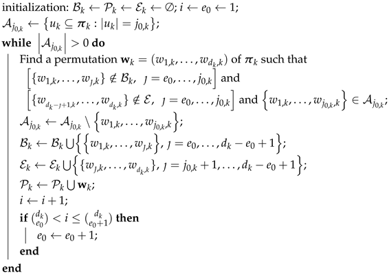Algorithm 1 provides the permutations selected (i.e., ${\mathcal{P}}_k$) that are used for deriving different DMs. For instance, if $d_2=3,{\mathit{\pi }}_2=\{1,2,3\}$, the permutations $(1,2,3)$ and $(3,2,1)$ lead to the following DMs:

$$(X_2,X_3)\stackrel{d}{=}{r}_1(X_1,Z_2,Z_3);(X_2,X_1)\stackrel{d}{=}{r}_3(X_3,Z_2,Z_1),$$

and the associated ERs, that is,

$$f\left(\mathbf{X}\right)\stackrel{d}{=}f(X_1,r_1(X_1,Z_2,Z_3));f\left(\mathbf{X}\right)\stackrel{d}{=}f(X_3,r_3(X_3,Z_2,Z_1)).$$

The set ${\mathcal{P}}_k$ from Algorithm 1 contains $\left(\genfrac{}{}{0pt}{}{d_k}{j_{0,k}}\right)$ permutations. The set ${\mathcal{B}}_k$ is built using ${\mathcal{P}}_k$, and it consists of sets containing the first ı elements of ${\mathbf{w}}_k$ for any $\iota \in \{1,\dots ,d_k\}$ and ${\mathbf{w}}_k\in {\mathcal{P}}_k$. Lemma 4 shows the properties of such sets.

Lemma 4.

Consider $j_{0,k}$ given by (14) and ${\mathcal{B}}_k,{\mathcal{P}}_k$ given by Algorithm 1. Then,

$${\mathcal{B}}_k=\left\{u\subseteq {\mathit{\pi }}_k:\forall \left|u\right|>0\right\};$$

(15)

$${\mathcal{B}}_k=\left\{\{w_{1,k},\dots ,w_{\iota ,k}\},\iota =1,\dots ,d_k:\forall {\mathbf{w}}_k\in {\mathcal{P}}_k\right\}.$$

(16)

Proof. 

See Appendix D. □

Based on Lemma 4, we quantify the necessary and sufficient number of ERs of f given ${\mathbf{X}}_u$ for all $u\subseteq \{1,\dots ,d\}$ in Theorem 1. For ${\mathbf{w}}_k\in {\mathcal{P}}_k$, recall that ${\mathbf{w}}_{\sim 1,k}$: = $(w_{2,k},\dots ,w_{d_k,k})$ and $\left|{\mathcal{P}}_k\right|=\left(\genfrac{}{}{0pt}{}{d_k}{j_{0,k}}\right)$ with $k=2,\dots ,K$.

Theorem 1.

Consider integers $p_2\le d_2,\dots ,p_K\le d_K$. Then, the minimum number of ERs of f given ${\mathbf{X}}_u$ for all $u\subseteq \{1,\dots ,d\}$ is

$$R_{min}:=\prod _{k=2}^K\left({\displaystyle \genfrac{}{}{0pt}{}{d_k}{j_{0,k}}}\right).$$

(17)

Such necessary and sufficient ERs are given by

$$\begin{array}{ccc}\hfill f\left(\mathbf{X},\theta \right)& \stackrel{d}{=}& g_{\mathcal{l}}\left({\mathbf{X}}_{{\mathit{\pi }}_1},X_{w_{1,2}},{\mathbf{Z}}_{{\mathbf{w}}_{\sim 1,2}},\dots ,X_{w_{1,K}},{\mathbf{Z}}_{{\mathbf{w}}_{\sim 1,K}},\theta \right),\hfill \end{array}$$

(18)

where $\mathcal{l}:=\left({\mathbf{w}}_2,\dots ,{\mathbf{w}}_K\right)$ for all ${\mathbf{w}}_k\in {\mathcal{P}}_k$ and $k=2,\dots ,K$.

Proof. 

See Appendix E. □

It is worth noting that each ER of Equation (18) shares the same distribution of $f\left(\mathbf{X},\theta \right)$, and two different ERs should be considered independent to avoid misleading dependencies. When a function includes only independent variables, we see that $R_{min}=1$. Reducing $R_{min}$ will depend on the analysis of interest one is going to perform. For instance, one ER is sufficient to determine the distribution of $f\left(\mathbf{X},\theta \right)$ conditional on ${\mathbf{X}}_u$ for all

$$u\in \left\{\{u_0,w_{1,k},\dots ,w_{\iota ,k}\}:\forall u_0\subseteq {\mathit{\pi }}_1,\forall \iota \in \{0,\dots ,d_k\},k=2,\dots ,K\right\}.$$

Likewise, $R_1=max(d_2,\dots ,d_K)$ ERs are used for assessing the main and total effects of $X_j$s for any $j\in \{1,\dots ,d\}$ in [16]. It is also worth noting that the above ERs can lead to assessing the effects of other inputs or groups of inputs.

Discussions About High-Dimensional Cases

Implementation of Algorithm 1 can be made fast for moderate values of each $d_k$, that is $d_k\le 10$ with $k=2,\dots ,K$. Since Algorithm 1 must be run separately for each ${\mathit{\pi }}_k$ with $k=2,\dots ,K$ and $d={\sum }_{k=1}^K{d}_k$, implementation of Algorithm 1 remains fast in high-dimensional settings, provided that each $d_k\le 10$ with $k=2,\dots ,K$. When there is $k_0\in \{2,\dots ,K\}$ such that $d_{k_0}>10$, Algorithm 1 can still be used with a substantial requirement of time to obtain all the necessary and sufficient permutations of ${\mathit{\pi }}_{k_0}$. But, as the selected permutations are not going to change for a given $d_k$ with $k\ge 2$, a table of selected permutations for different values of $d_k$ will avoid tuning this algorithm all the time.

Regarding the $R_{min}$ ERs, we can check that $2^K=2^{\frac{d-d_1}{2}}\le R_{min}\le 2^{d-d_1}$ because $\left(\genfrac{}{}{0pt}{}{d_k}{j_{0,k}}\right)=\left(\genfrac{}{}{0pt}{}{d_k}{\left[\frac{d_k}{2}\right]}\right)\le 2^{d_k}$ with $\left[{\displaystyle \frac{d_k}{2}}\right]$ the largest integer that is less than ${\displaystyle \frac{d_k}{2}}$. Thus, computing all the effects of inputs will require at least $2^{\frac{d-d_1}{2}}$ ERs and at most $2^{d-d_1}$ ERs, which grow exponentially with respect to $d(1-\alpha )$ with $\alpha :={\displaystyle \frac{d_1}{d}}\in [0,1]$. If the effects of ${\mathbf{X}}_{{\mathit{\pi }}_{k_0}}$ are not significant, then $\alpha =\frac{d_1+d_{k_0}}{d}$. Based on the values of $\alpha$, different conclusions can be drawn.

4. Dependent Multivariate Sensitivity Analysis

This section extends dependent generalized sensitivity indices (dGSIs) for models with NIVVs introduced in [16] by defining the dGSIs for every subset of inputs and for functional outputs. Since the ER given by Equation (18) includes only independent variables, we define dGSIs by relying on the multivariate sensitivity analysis ([2,3,4,44,45]). To ensure that the proposed dGSIs in this section are well defined, assume that

(A1): ${\displaystyle 0<{\int }_{\Theta }\mathbb{E}\left[{\left|\left|f\left(\mathbf{X},\theta \right)\right|\right|}_{L^2}^2\right]d\theta <+\infty }$.

Definitions of GSIs and dGSIs are based on sensitivity functionals (SFs), which contain information about the single and overall contributions of input variables over the whole functional outputs [2,6,16,46]. To define SFs, recall that $0\le p_k\le d_k$, ${\mathbf{v}}_k=(w_{2,k},\dots ,w_{p_k,k})$ and ${\mathbf{u}}_k=(w_{1,k},{\mathbf{v}}_k)$ with $k=2,\dots ,K$, and define ${\overline{\mathbf{u}}}_k:=\left(w_{p_k+1,k},\dots ,w_{d_k,k}\right)$. According to Lemmas 3 and 4, for all $u\subseteq \{1,\dots ,d\}$, there exists $u_0\subseteq {\mathit{\pi }}_1$, a vector ${\mathbf{w}}_k\in {\mathcal{P}}_k$ and $p_k$ with $k=2,\dots ,K$ such that ${\mathbf{X}}_u=\left({\mathbf{X}}_{u_0},{\mathbf{X}}_{{\mathbf{u}}_2},\dots ,{\mathbf{X}}_{{\mathbf{u}}_K}\right)$ and

$$f(\mathbf{X},\theta )|{\mathbf{X}}_u\stackrel{d}{=}{g}_{\mathcal{l}}\left({\mathbf{X}}_{{\mathit{\pi }}_1},X_{w_{1,2}},{\mathbf{Z}}_{{\mathbf{w}}_{\sim 1,2}},\dots ,X_{w_{1,K}},{\mathbf{Z}}_{{\mathbf{w}}_{\sim 1,K}},\theta \right)|{\mathbf{X}}_{u_0},{\mathbf{R}}_{{\mathbf{u}}_2},\dots ,{\mathbf{R}}_{{\mathbf{u}}_K},$$

where ${\mathbf{R}}_{{\mathbf{u}}_k}:=(X_{w_1,k},{\mathbf{Z}}_{{\mathbf{v}}_k})$, $k=2,\dots ,K$. Thus, the effects of inputs ${\mathbf{X}}_u$ are equal to the effects of ${\mathbf{X}}_{u_0},{\mathbf{R}}_{{\mathbf{u}}_2},\dots ,{\mathbf{R}}_{{\mathbf{u}}_K}$ using $g_{\mathcal{l}}$. For concise notations, we use

$${\mathbf{X}}_{\{{\mathit{\pi }}_1,\mathbf{s}\}}:=\left(X_j,\forall j\in \{{\mathit{\pi }}_1,\mathbf{s}\}\right);{\mathbf{Z}}_{{\mathbf{w}}_{\sim 1}}=\left({\mathbf{Z}}_{{\mathbf{w}}_{\sim 1,2}},\dots ,{\mathbf{Z}}_{{\mathbf{w}}_{\sim 1,K}}\right),$$

$${\mathbf{R}}_u:=\left({\mathbf{X}}_{u_0},{\mathbf{R}}_{{\mathbf{u}}_2},\dots ,{\mathbf{R}}_{{\mathbf{u}}_K}\right);{\mathbf{R}}_{\sim u}:=\left({\mathbf{X}}_{{\mathit{\pi }}_1\setminus u_0},{\mathbf{Z}}_{{\overline{\mathbf{u}}}_2},\dots ,{\mathbf{Z}}_{{\overline{\mathbf{u}}}_K}\right).$$

Note that $\mathbf{R}:=({\mathbf{R}}_u,{\mathbf{R}}_{\sim u})$ is a partition of $\left({\mathbf{X}}_{\{{\mathit{\pi }}_1,\mathbf{s}\}},{\mathbf{Z}}_{{\mathbf{w}}_{\sim 1}}\right)$.

The first-order SF of ${\mathbf{X}}_u$ with $u=\left\{u_0,{\mathbf{u}}_2,\dots ,{\mathbf{u}}_K\right\}$ is given by

$$f_u^{fo}\left({\mathbf{R}}_u,\theta \right):=\mathbb{E}\left[g_{\mathcal{l}}\left({\mathbf{X}}_{\{{\mathit{\pi }}_1,\mathbf{s}\}},{\mathbf{Z}}_{{\mathbf{w}}_{\sim 1}},\theta \right)\mathcal{|}{\mathbf{R}}_u\right]-\mathbb{E}\left[g_{\mathcal{l}}\left({\mathbf{X}}_{\{{\mathit{\pi }}_1,\mathbf{s}\}},{\mathbf{Z}}_{{\mathbf{w}}_{\sim 1}},\theta \right)\right],$$

(19)

and the total SF, which contains the overall information about ${\mathbf{X}}_u$, is given by

$$f_u^{tot}\left({\mathbf{X}}_{\{{\mathit{\pi }}_1,\mathbf{s}\}},{\mathbf{Z}}_{{\mathbf{w}}_{\sim 1}},\theta \right):=g_{\mathcal{l}}\left({\mathbf{X}}_{\{{\mathit{\pi }}_1,\mathbf{s}\}},{\mathbf{Z}}_{{\mathbf{w}}_{\sim 1}},\theta \right)-{\mathbb{E}}_{{\mathbf{R}}_u}\left[g_{\mathcal{l}}\left({\mathbf{X}}_{\{{\mathit{\pi }}_1,\mathbf{s}\}},{\mathbf{Z}}_{{\mathbf{w}}_{\sim 1}},\theta \right)\right],$$

(20)

where ${\mathbb{E}}_{{\mathbf{R}}_u}$ means that the expectation is taken with respect to ${\mathbf{R}}_u$. The SFs given by (19) and (20) are random processes, and their components may be correlated and/or dependent. Using the variance–covariance as an importance measure, the definitions of dGSIs rely on the cross-covariances of SFs. For ${\theta }_1,{\theta }_2\in \Theta$, the first-order cross-covariance or the cross-covariance of $f_u^{fo}$ is given by

$${\Sigma }_u({\theta }_1,{\theta }_2):=\mathbb{E}\left[f_u^{fo}\left({\mathbf{R}}_u,{\theta }_1\right)f_u^{fo}{\left({\mathbf{R}}_u,{\theta }_2\right)}^T\right].$$

Furthermore, the cross-covariances of $f_u^{tot}$ and f are given as follows:

$${\Sigma }_u^{tot}({\theta }_1,{\theta }_2):=\mathbb{E}\left[f_u^{tot}\left({\mathbf{X}}_{\{{\mathit{\pi }}_1,\mathbf{s}\}},{\mathbf{Z}}_{{\mathbf{w}}_{\sim 1}},{\theta }_1\right)f_u^{tot}{\left({\mathbf{X}}_{\{{\mathit{\pi }}_1,\mathbf{s}\}},{\mathbf{Z}}_{{\mathbf{w}}_{\sim 1}},{\theta }_2\right)}^T\right],$$

$$\begin{array}{ccc}\hfill \Sigma ({\theta }_1,{\theta }_2)& :=& \mathbb{E}\left[g_{\mathcal{l}}\left({\mathbf{X}}_{\{{\mathit{\pi }}_1,\mathbf{s}\}},{\mathbf{Z}}_{{\mathbf{w}}_{\sim 1}},{\theta }_1\right)g_{\mathcal{l}}{\left({\mathbf{X}}_{\{{\mathit{\pi }}_1,\mathbf{s}\}},{\mathbf{Z}}_{{\mathbf{w}}_{\sim 1}},{\theta }_2\right)}^T\right]\hfill \\ & & -\mathbb{E}\left[g_{\mathcal{l}}\left({\mathbf{X}}_{\{{\mathit{\pi }}_1,\mathbf{s}\}},{\mathbf{Z}}_{{\mathbf{w}}_{\sim 1}},{\theta }_1\right)\right]\mathbb{E}\left[g_{\mathcal{l}}{\left({\mathbf{X}}_{\{{\mathit{\pi }}_1,\mathbf{s}\}},{\mathbf{Z}}_{{\mathbf{w}}_{\sim 1}},{\theta }_2\right)}^T\right].\hfill \end{array}$$

To account for the different properties of the aforementioned SFs, we distinguish three different types of dGSIs.

Definition 3. 

Consider the cross-covariances of SFs, and assume that (A1) holds.

(i) 

For the first-type dGSIs, the first-order and total indices are given by

$${\displaystyle dGS{I}_{u,1}:=\frac{{\int }_{\Theta }Tr\left({\Sigma }_u(\theta ,\theta )\right)d\theta }{{\int }_{\Theta }Tr\left(\Sigma (\theta ,\theta )\right)d\theta },dGS{I}_{T_u,1}:=\frac{{\int }_{\Theta }Tr\left({\Sigma }_u^{tot}(\theta ,\theta )\right)d\theta }{{\int }_{\Theta }Tr\left(\Sigma (\theta ,\theta )\right)d\theta }.}$$

(21)

(ii) 

The second-type dGSIs are defined as follows:

$${\displaystyle dGS{I}_{u,2}:={\left(\frac{{\int }_{\Theta }{\left|\left|{\Sigma }_u(\theta ,\theta )\right|\right|}_F^{2}d\theta }{{\int }_{\Theta }{\left|\left|\Sigma (\theta ,\theta )\right|\right|}_F^{2}d\theta }\right)}^{1/2},dGS{I}_{T_u,2}:={\left(\frac{{\int }_{\Theta }{\left|\left|{\Sigma }_u^{tot}(\theta ,\theta )\right|\right|}_F^{2}d\theta }{{\int }_{\Theta }{\left|\left|\Sigma (\theta ,\theta )\right|\right|}_F^{2}d\theta }\right)}^{1/2}.}$$

(22)

(iii) 

The third-type dGSIs are given as follows:

$${\displaystyle dGS{I}_{u,3}:={\left(\frac{{\int }_{{\Theta }^2}{\left|\left|{\Sigma }_u({\theta }_1,{\theta }_2)\right|\right|}_F^{2}d{\theta }_{1}d{\theta }_2}{{\int }_{{\Theta }^2}{\left|\left|\Sigma ({\theta }_1,{\theta }_2)\right|\right|}_F^{2}d{\theta }_{1}d{\theta }_2}\right)}^{1/2},dGS{I}_{T_u,3}:={\left(\frac{{\int }_{{\Theta }^2}{\left|\left|{\Sigma }_u^{tot}({\theta }_1,{\theta }_2)\right|\right|}_F^{2}d{\theta }_{1}d{\theta }_2}{{\int }_{{\Theta }^2}{\left|\left|\Sigma ({\theta }_1,{\theta }_2)\right|\right|}_F^{2}d{\theta }_{1}d{\theta }_2}\right)}^{1/2}.}$$

(23)

The first-type and the second-type dGSIs treat independently the outputs $f(\mathbf{X},{\theta }_1)$ and $f(\mathbf{X},{\theta }_2)$ when ${\theta }_1\ne {\theta }_2$, but the second-type dGSIs account for the correlations among the components of SFs from the same output $f(\mathbf{X},\theta )$. Furthermore, the third-type dGSIs account for the correlations among the cross-components of SFs.

4.1. Properties of Dependent Generalized Sensitivity Indices

The two types of dGSIs share the same properties as those proposed in [16] for $0\le p_k\le 1$, only. Proposition 2 extends such properties for all $p_k\in \{0,\dots ,d_k\}$.

Proposition 2.

Under (A1), consider the dGSIs of Definition 3. Then,

$$0\le dGS{I}_{u,1}\le dGS{I}_{T_u,1}\le 1;0\le dGS{I}_{u,2}\le dGS{I}_{T_u,2}\le 1.$$

Moreover, if the cross-covariances are positive semi-definite, then we have

$$0\le dGS{I}_{u,3}\le dGS{I}_{T_u,3}\le 1.$$

Proof. 

See Appendix F. □

When the total dGSI of ${\mathbf{X}}_u=\left({\mathbf{X}}_{u_0},{\mathbf{X}}_{u_1},\dots ,{\mathbf{X}}_{u_K}\right)$ is zero or almost zero (i.e., $dGS{I}_{T_u,•}\approx 0$), we have to fix ${\mathbf{X}}_u$ using the DM associated with each ${\mathbf{X}}_{{\mathit{\pi }}_k}$, $k=2,\dots ,K$. Indeed, for the DM ${\mathbf{X}}_{u_k}=r_{\sim u_k}({\mathbf{X}}_{\sim u_k},{\mathbf{Z}}_{u_k}))$, fixing ${\mathbf{X}}_{u_K}$ comes down to fix ${\mathbf{Z}}_{u_k}$ to its nominal values. Since we can compute the total $dGSI$ of each block of NIVs, that is, ${\mathbf{X}}_{{\mathit{\pi }}_k}$ using any ER of f, it becomes possible to quickly identify the non-influential block of NIVs, and then put our computational efforts on the most important groups of NIVs.

Remark 1.

Given $j_1,j_2\in \{1,\dots ,d\}$, the same rankings of the inputs $X_{j_1}$ and $X_{j_2}$ using either $dGS{I}_{T_j,1}$ or $dGS{I}_{T_j,2}$ with $j\in \{j_1,j_2\}$ are obtained under the assumptions ${\Sigma }_{j_1}^{tot}(\theta ,\theta )⪯{\Sigma }_{j_2}^{tot}(\theta ,\theta )$ or ${\Sigma }_{j_2}^{tot}(\theta ,\theta )⪯{\Sigma }_{j_1}^{tot}(\theta ,\theta )$. Note that ${\mathcal{A}}_1⪯{\mathcal{A}}_2$ means that ${\mathcal{A}}_2-{\mathcal{A}}_1$ is a positive semi-definite matrix, a.k.a. the Loewner partial ordering between matrices (see also Section 6.3 in [16]).

Remark 2.

Case of the multivariate dynamic function

Consider a model that is evaluated at $\mathbf{X}$ and provides n dynamic(s), such as a spatiotemporal model. Such a model is a particular case of multivariate and functional outputs. Indeed, the multivariate dynamic model given by $f:{\mathbb{R}}^d\times [0,T]\to {\mathbb{R}}^n$ and $f(\mathbf{X},t)\in {\mathbb{R}}^n$ with $t\in [0,T]$ is mathematically identical to $f(\mathbf{X},\theta )$ using $\Theta =[0,T]$ and $\theta =t$.

4.2. Case of the Multivariate Response Models

When $\Theta =\left\{{\theta }_0\right\}$, the multivariate and functional outputs come down to $f(\mathbf{X},{\theta }_0)=:h\left(\mathbf{X}\right)$ with h: ${\mathbb{R}}^d\to {\mathbb{R}}^n$. Thus, the dGSIs of Definition 3 can be adapted for quantifying the effect of inputs. It is worth noting that the third-type dGSIs are equal to the second-type dGSIs, and both types of dGSIs boil down to the second-type dGSIs provided in Definition 4. Moreover, the cross-covariances become the covariances, and we use ${\Sigma }_u$: = ${\Sigma }_u({\theta }_0,{\theta }_0)$, ${\Sigma }_u^{tot}$: = ${\Sigma }_u^{tot}({\theta }_0,{\theta }_0)$ and $\Sigma$: = $\Sigma ({\theta }_0,{\theta }_0)$.

Definition 4.

Consider the above covariances of SFs and assume (A1) holds.

(i) 

The first-type dGSIs for a given multivariate response function are

$$dGS{I}_{u,1}^M:={\displaystyle \frac{Tr\left({\Sigma }_u\right)}{Tr\left(\Sigma \right)}},dGS{I}_{T_u,1}^M:={\displaystyle \frac{Tr\left({\Sigma }_u^{tot}\right)}{Tr\left(\Sigma \right)}}.$$

(24)

(ii) 

The second-type dGSIs are defined as follows:

$$dGS{I}_{u,2}^M:={\displaystyle \frac{{\left|\left|{\Sigma }_u\right|\right|}_F}{{\left|\left|\Sigma \right|\right|}_F}},dGS{I}_{T_u,2}^M:={\displaystyle \frac{{\left|\left|{\Sigma }_u^{tot}\right|\right|}_F}{{\left|\left|\Sigma \right|\right|}_F}}.$$

(25)

Also, in the case where $n=1$, the two types of dGSIs of Definition 4 are equal and boil down to dependent sensitivity indices (dSIs) for single-response models (see Definition 5).

Definition 5.

For a function $f:{\mathbb{R}}^d\to \mathbb{R}$ ($n=1$), the dSIs of ${\mathbf{X}}_u$ are given by

$$d{S}_u:={\displaystyle \frac{{\Sigma }_u}{\Sigma }},d{S}_{T_u}:={\displaystyle \frac{{\Sigma }_u^{tot}}{\Sigma }}.$$

(26)

5. Estimators of Dependent Generalized Sensitivity Indices

In this section, we provide unbiased estimators of the cross-covariances and covariances of SFs, consistent estimators of dGSIs, and their asymptotic distributions. For the sake of simplicity, we provide estimators of covariances and dGSIs using the functions $g_{\mathcal{l}}$ that include only independent variables, that is, ${\mathbf{X}}_{\{{\mathit{\pi }}_1,\mathbf{s}\}},{\mathbf{Z}}_{{\mathbf{w}}_{\sim 1}}$ Note that the Supplementary Materials provides such estimators using f directly thanks to the relation

$$\begin{array}{ccc}\hfill g_{\mathcal{l}}\left({\mathbf{X}}_{\{{\mathit{\pi }}_1,\mathbf{s}\}},{\mathbf{Z}}_{{\mathbf{w}}_{\sim 1}},\theta \right)& =& f\left({\mathbf{X}}_{\{{\mathit{\pi }}_1,\mathbf{s}\}},r_{\mathbf{s}}\left({\mathbf{X}}_{\mathbf{s}},{\mathbf{Z}}_{{\mathbf{w}}_{\sim 1}}\right),\theta \right)\hfill \\ & =& f\left({\mathbf{X}}_{\{{\mathit{\pi }}_1,\mathbf{s}\}},r_{w_{1,2}}(X_{w_{1,2}},{\mathbf{Z}}_{{\mathbf{w}}_{\sim 1,2}}),\dots ,r_{w_{1,K}}(X_{w_{1,K}},{\mathbf{Z}}_{{\mathbf{w}}_{\sim 1,K}}),\theta \right).\hfill \end{array}$$

To derive the estimators of cross-covariances that are useful for computing dGSIs, we are given two i.i.d. samples from $\left({\mathbf{X}}_{\{{\mathit{\pi }}_1,\mathbf{s}\}},{\mathbf{Z}}_{{\mathbf{w}}_{\sim 1}}\right)$, that is, ${\left\{\left({\mathbf{X}}_{i,\{{\mathit{\pi }}_1,\mathbf{s}\}}^{\left(1\right)},{\mathbf{Z}}_{i,{\mathbf{w}}_{\sim 1}}^{\left(1\right)}\right)\right\}}_{i=1}^m$ and ${\left\{\left({\mathbf{X}}_{i,\{{\mathit{\pi }}_1,\mathbf{s}\}}^{\left(2\right)},{\mathbf{Z}}_{i,{\mathbf{w}}_{\sim 1}}^{\left(2\right)}\right)\right\}}_{i=1}^m$, and we use ${\mathbf{X}}_i^{\left(k\right)}:=\left({\mathbf{X}}_{i,\{{\mathit{\pi }}_1,\mathbf{s}\}}^{\left(k\right)},r_{\mathbf{s}}\left({\mathbf{X}}_{i,\mathbf{s}}^{\left(k\right)},{\mathbf{Z}}_{i,{\mathbf{w}}_{\sim 1}}^{\left(k\right)}\right)\right)$, $k=1,2$, $i=1,\dots ,m$. Since $\mathbf{R}:=({\mathbf{R}}_u,{\mathbf{R}}_{\sim \mathbf{u}})$ is a partition of $\left({\mathbf{X}}_{\{{\mathit{\pi }}_1,\mathbf{s}\}},{\mathbf{Z}}_{{\mathbf{w}}_{\sim 1}}\right)$, we can deduce the following two i.i.d. samples: ${\left\{{\mathbf{R}}_i^{\left(1\right)}:=\left({\mathbf{R}}_{i,u}^{\left(1\right)},{\mathbf{R}}_{\mathbf{i},\sim \mathbf{u}}^{\left(1\right)}\right)\right\}}_{i=1}^m$ and ${\left\{{\mathbf{R}}_i^{\left(2\right)}:=\left({\mathbf{R}}_{i,u}^{\left(2\right)},{\mathbf{R}}_{\mathbf{i},\sim \mathbf{u}}^{\left(2\right)}\right)\right\}}_{i=1}^m$.

Theorem 2.

Assume (A1) holds. Then, unbiased and consistent estimators of ${\Sigma }_u({\theta }_1,{\theta }_2)$, ${\Sigma }_u^{tot}({\theta }_1,{\theta }_2)$ and $\Sigma ({\theta }_1,{\theta }_2)$ are, respectively, given by

$$\begin{array}{ccc}\hfill & & \widehat{{\Sigma }_u({\theta }_1,{\theta }_2)}:={\displaystyle \frac{1}{2m}}\sum _{i=1}^m\hfill \\ & & \left[g_{\mathcal{l}}\left({\mathbf{R}}_i^{\left(1\right)},{\theta }_1\right)-g_{\mathcal{l}}\left({\mathbf{R}}_{i,u}^{\left(2\right)},{\mathbf{R}}_{i,\sim u}^{\left(1\right)},{\theta }_1\right)\right]{\left[g_{\mathcal{l}}\left({\mathbf{R}}_{i,u}^{\left(1\right)},{\mathbf{R}}_{i,\sim u}^{\left(2\right)},{\theta }_2\right)-g_{\mathcal{l}}\left({\mathbf{R}}_i^{\left(2\right)},{\theta }_2\right)\right]}^T;\hfill \end{array}$$

$$\begin{array}{ccc}\hfill & & \widehat{{\Sigma }_u^{tot}({\theta }_1,{\theta }_2)}:={\displaystyle \frac{1}{2m}}\sum _{i=1}^m\hfill \\ & & \left[g_{\mathcal{l}}\left({\mathbf{R}}_i^{\left(1\right)},{\theta }_1\right)-g_{\mathcal{l}}\left({\mathbf{R}}_{i,u}^{\left(2\right)},{\mathbf{R}}_{i,\sim u}^{\left(1\right)},{\theta }_1\right)\right]{\left[g_{\mathcal{l}}\left({\mathbf{R}}_{i,u}^{\left(1\right)},{\mathbf{R}}_{i,\sim u}^{\left(1\right)},{\theta }_2\right)-g_{\mathcal{l}}\left({\mathbf{R}}_{i,u}^{\left(2\right)},{\mathbf{R}}_{i,\sim u}^{\left(1\right)},{\theta }_2\right)\right]}^T;\hfill \end{array}$$

$$\begin{array}{ccc}\hfill \widehat{\Sigma ({\theta }_1,{\theta }_2)}& :=& {\displaystyle \frac{1}{2m}}\sum _{i=1}^m\left[g_{\mathcal{l}}\left({\mathbf{R}}_i^{\left(1\right)},{\theta }_1\right)-g_{\mathcal{l}}\left({\mathbf{R}}_i^{\left(2\right)},{\theta }_1\right)\right]{\left[g_{\mathcal{l}}\left({\mathbf{R}}_i^{\left(1\right)},{\theta }_2\right)-g_{\mathcal{l}}\left({\mathbf{R}}_i^{\left(2\right)},{\theta }_2\right)\right]}^T\hfill \\ & & ={\displaystyle \frac{1}{2m}}\sum _{i=1}^m\left[f\left({\mathbf{X}}_i^{\left(1\right)},{\theta }_1\right)-f\left({\mathbf{X}}_i^{\left(2\right)},{\theta }_1\right)\right]{\left[f\left({\mathbf{X}}_i^{\left(1\right)},{\theta }_2\right)-f\left({\mathbf{X}}_i^{\left(2\right)},{\theta }_2\right)\right]}^T.\hfill \end{array}$$

Proof. 

See Appendix G. □

Note that when ${\theta }_1={\theta }_2=\theta$, the estimators provided in Theorem 2 are minimum-variance unbiased estimators (MVUEs). Using Theorem 2, we deduce the estimators of the variance–covariances of SFs for the multivariate response models and single-response models. To provide such results for the vector-valued function $f:{\mathbb{R}}^d\to {\mathbb{R}}^n$ in Corollary 1, let us consider the following symmetric kernels:

$$\begin{array}{ccc}\hfill K_u^{fo}\left({\mathbf{R}}_i^{\left(1\right)},{\mathbf{R}}_i^{\left(2\right)}\right)& :=& \left[g_{\mathcal{l}}\left({\mathbf{R}}_i^{\left(1\right)}\right)-g_{\mathcal{l}}\left({\mathbf{R}}_{i,u}^{\left(2\right)},{\mathbf{R}}_{i,\sim u}^{\left(1\right)}\right)\right]{\left[g_{\mathcal{l}}\left({\mathbf{R}}_{i,u}^{\left(1\right)},{\mathbf{R}}_{i,\sim u}^{\left(2\right)}\right)-g_{\mathcal{l}}\left({\mathbf{R}}_i^{\left(2\right)}\right)\right]}^T\hfill \\ & & +\left[g_{\mathcal{l}}\left({\mathbf{R}}_{i,u}^{\left(1\right)},{\mathbf{R}}_{i,\sim u}^{\left(2\right)}\right)-g_{\mathcal{l}}\left({\mathbf{R}}_i^{\left(2\right)}\right)\right]{\left[g_{\mathcal{l}}\left({\mathbf{R}}_i^{\left(1\right)}\right)-g_{\mathcal{l}}\left({\mathbf{R}}_{i,u}^{\left(2\right)},{\mathbf{R}}_{i,\sim u}^{\left(1\right)}\right)\right]}^T;\hfill \end{array}$$

$$\begin{array}{ccc}\hfill K_u^{tot}\left({\mathbf{R}}_i^{\left(1\right)},{\mathbf{R}}_i^{\left(2\right)}\right)& :=& \left[g_{\mathcal{l}}\left({\mathbf{R}}_i^{\left(1\right)}\right)-g_{\mathcal{l}}\left({\mathbf{R}}_{i,u}^{\left(2\right)},{\mathbf{R}}_{i,\sim u}^{\left(1\right)}\right)\right]{\left[g_{\mathcal{l}}\left({\mathbf{R}}_i^{\left(1\right)}\right)-g_{\mathcal{l}}\left({\mathbf{R}}_{i,u}^{\left(2\right)},{\mathbf{R}}_{i,\sim u}^{\left(1\right)}\right)\right]}^T\hfill \\ & & +\left[g_{\mathcal{l}}\left({\mathbf{R}}_{i,u}^{\left(1\right)},{\mathbf{R}}_{i,\sim u}^{\left(2\right)}\right)-g_{\mathcal{l}}\left({\mathbf{R}}_i^{\left(2\right)}\right)\right]{\left[g_{\mathcal{l}}\left({\mathbf{R}}_{i,u}^{\left(1\right)},{\mathbf{R}}_{i,\sim u}^{\left(2\right)}\right)-g_{\mathcal{l}}\left({\mathbf{R}}_i^{\left(2\right)}\right)\right]}^T;\hfill \end{array}$$

$$\begin{array}{ccc}\hfill K\left({\mathbf{R}}_i^{\left(1\right)},{\mathbf{R}}_i^{\left(2\right)}\right)& :=& \left[g_{\mathcal{l}}\left({\mathbf{R}}_{i,u}^{\left(1\right)},{\mathbf{R}}_{i,\sim u}^{\left(2\right)}\right)-g_{\mathcal{l}}\left({\mathbf{R}}_{i,u}^{\left(2\right)},{\mathbf{R}}_{i,\sim u}^{\left(1\right)}\right)\right]{\left[g_{\mathcal{l}}\left({\mathbf{R}}_{i,u}^{\left(1\right)},{\mathbf{R}}_{i,\sim u}^{\left(2\right)}\right)-g_{\mathcal{l}}\left({\mathbf{R}}_{i,u}^{\left(2\right)},{\mathbf{R}}_{i,\sim u}^{\left(1\right)}\right)\right]}^T\hfill \\ & & +\left[g_{\mathcal{l}}\left({\mathbf{R}}_i^{\left(1\right)}\right)-g_{\mathcal{l}}\left({\mathbf{R}}_i^{\left(2\right)}\right)\right]{\left[g_{\mathcal{l}}\left({\mathbf{R}}_i^{\left(1\right)}\right)-g_{\mathcal{l}}\left({\mathbf{R}}_i^{\left(2\right)}\right)\right]}^T.\hfill \end{array}$$

Corollary 1.

Assume that f has finite fourth moments (i.e., (A2)) and (A1) hold. Then, the MVUEs and consistent estimators of the covariance matrices ${\Sigma }_u$, ${\Sigma }_u^{tot}$, and Σ are, respectively, given by

$$\widehat{{\Sigma }_u}:={\displaystyle \frac{1}{4m}}\sum _{i=1}^m{K}_u^{fo}\left({\mathbf{R}}_i^{\left(1\right)},{\mathbf{R}}_i^{\left(2\right)}\right),\widehat{{\Sigma }_u^{tot}}:={\displaystyle \frac{1}{4m}}\sum _{i=1}^m{K}_u^{tot}\left({\mathbf{R}}_i^{\left(1\right)},{\mathbf{R}}_i^{\left(2\right)}\right);$$

$$\widehat{\Sigma }:={\displaystyle \frac{1}{4m}}\sum _{i=1}^{m}K\left({\mathbf{R}}_i^{\left(1\right)},{\mathbf{R}}_i^{\left(2\right)}\right).$$

Proof. 

See Appendix H. □

For single-response models (i.e., $n=1$), the MVUEs of the covariances of SFs in Corollary 1 have simple expressions, given below.

Corollary 2.

Under the assumptions (A1)-(A2) and $n=1$, the MVUEs $\widehat{{\Sigma }_u}$, $\widehat{{\Sigma }_u^{tot}}$, and $\widehat{\Sigma }$ become, respectively,

$$\widehat{{\sigma }_u}:={\displaystyle \frac{1}{2m}}\sum _{i=1}^m\left[g_{\mathcal{l}}\left({\mathbf{R}}_i^{\left(1\right)}\right)-g_{\mathcal{l}}\left({\mathbf{R}}_{i,u}^{\left(2\right)},{\mathbf{R}}_{i,\sim u}^{\left(1\right)}\right)\right]\left[g_{\mathcal{l}}\left({\mathbf{R}}_{i,u}^{\left(1\right)},{\mathbf{R}}_{i,\sim u}^{\left(2\right)}\right)-g_{\mathcal{l}}\left({\mathbf{R}}_i^{\left(2\right)}\right)\right];$$

$$\widehat{{\sigma }_u^{tot}}:={\displaystyle \frac{1}{4m}}\sum _{i=1}^m\left\{{\left[g_{\mathcal{l}}\left({\mathbf{R}}_i^{\left(1\right)}\right)-g_{\mathcal{l}}\left({\mathbf{R}}_{i,u}^{\left(2\right)},{\mathbf{R}}_{i,\sim u}^{\left(1\right)}\right)\right]}^2+{\left[g_{\mathcal{l}}\left({\mathbf{R}}_{i,u}^{\left(1\right)},{\mathbf{R}}_{i,\sim u}^{\left(2\right)}\right)-g_{\mathcal{l}}\left({\mathbf{R}}_i^{\left(2\right)}\right)\right]}^2\right\};$$

$$\widehat{\sigma }:={\displaystyle \frac{1}{4m}}\sum _{i=1}^m\left\{{\left[g_{\mathcal{l}}\left({\mathbf{R}}_i^{\left(1\right)}\right)-g_{\mathcal{l}}\left({\mathbf{R}}_i^{\left(2\right)}\right)\right]}^2+{\left[g_{\mathcal{l}}\left({\mathbf{R}}_{i,u}^{\left(1\right)},{\mathbf{R}}_{i,\sim u}^{\left(2\right)}\right)-g_{\mathcal{l}}\left({\mathbf{R}}_{i,u}^{\left(2\right)},{\mathbf{R}}_{i,\sim u}^{\left(1\right)}\right)\right]}^2\right\}.$$

If we are only interested in the total effects, we should use the expressions of $\widehat{{\Sigma }_u^{tot}}$ and $\widehat{{\sigma }_u^{tot}}$ given, respectively, by

$${\displaystyle \frac{1}{2m}}\sum _{i=1}^m\left[g_{\mathcal{l}}\left({\mathbf{R}}_i^{\left(1\right)}\right)-g_{\mathcal{l}}\left({\mathbf{R}}_{i,u}^{\left(2\right)},{\mathbf{R}}_{i,\sim u}^{\left(1\right)}\right)\right]{\left[g_{\mathcal{l}}\left({\mathbf{R}}_i^{\left(1\right)}\right)-g_{\mathcal{l}}\left({\mathbf{R}}_{i,u}^{\left(2\right)},{\mathbf{R}}_{i,\sim u}^{\left(1\right)}\right)\right]}^T;$$

$${\displaystyle \frac{1}{2m}}\sum _{i=1}^m{\left[g_{\mathcal{l}}\left({\mathbf{R}}_i^{\left(1\right)}\right)-g_{\mathcal{l}}\left({\mathbf{R}}_{i,u}^{\left(2\right)},{\mathbf{R}}_{i,\sim u}^{\left(1\right)}\right)\right]}^2.$$

Using the results from Theorem 2, Corollary 1, and Corollary 2, we derive the estimators of dGSIs and dSIs in Corollary 3, Theorem 3, and Corollary 4, respectively.

Corollary 3.

Assume that (A1) and (A2) hold. If we observe the model outputs at ${\theta }_{\mathcal{l}}\in \Theta$ with $\mathcal{l}=1,\dots ,L$, then

(i) 

the consistent estimators of the first-type dGSIs are given as follows:

$${\displaystyle \widehat{dGS{I}_{u,1}}:=\frac{{\sum }_{\mathcal{l}=1}^{L}Tr\left(\widehat{{\Sigma }_u({\theta }_{\mathcal{l}},{\theta }_{\mathcal{l}})}\right)}{{\sum }_{\mathcal{l}=1}^{L}Tr\left(\widehat{\Sigma ({\theta }_{\mathcal{l}},{\theta }_{\mathcal{l}})}\right)}\stackrel{\mathcal{P}}{\to }dGS{I}_{u,1},}$$

when $L\to \infty ,m\to \infty$, where $\stackrel{\mathcal{P}}{\to }$ denotes the convergence in probability.

$${\displaystyle \widehat{dGS{I}_{T_u,1}}:=\frac{{\sum }_{\mathcal{l}=1}^{L}Tr\left(\widehat{{\Sigma }_u^{tot}({\theta }_{\mathcal{l}},{\theta }_{\mathcal{l}})}\right)}{{\sum }_{\mathcal{l}=1}^{L}Tr\left(\widehat{\Sigma ({\theta }_{\mathcal{l}},{\theta }_{\mathcal{l}})}\right)}\stackrel{\mathcal{P}}{\to }dGS{I}_{T_u,1}.}$$

(ii) 

The estimators of the second-type dGSIs are given as follows:

$${\displaystyle \widehat{dGS{I}_{u,2}}:={\left(\frac{{\sum }_{\mathcal{l}=1}^L{\left|\left|\widehat{{\Sigma }_u({\theta }_{\mathcal{l}},{\theta }_{\mathcal{l}})}\right|\right|}_F^2}{{\sum }_{\mathcal{l}=1}^L{\left|\left|\widehat{\Sigma ({\theta }_{\mathcal{l}},{\theta }_{\mathcal{l}})}\right|\right|}_F^2}\right)}^{1/2}\stackrel{\mathcal{P}}{\to }dGS{I}_{u,2},}$$

$${\displaystyle \widehat{dGS{I}_{T_u,2}}:={\left(\frac{{\sum }_{\mathcal{l}=1}^L{\left|\left|\widehat{{\Sigma }_u^{tot}({\theta }_{\mathcal{l}},{\theta }_{\mathcal{l}})}\right|\right|}_F^2}{{\sum }_{\mathcal{l}=1}^L{\left|\left|\widehat{\Sigma ({\theta }_{\mathcal{l}},{\theta }_{\mathcal{l}})}\right|\right|}_F^2}\right)}^{1/2}\stackrel{\mathcal{P}}{\to }dGS{I}_{T_u,2},}$$

(iii) 

The estimators of the third-type dGSIs are given as follows:

$${\displaystyle \widehat{dGS{I}_{u,3}}:={\left(\frac{{\sum }_{{\mathcal{l}}_1=1}^L{\sum }_{{\mathcal{l}}_2=1}^L{\left|\left|\widehat{{\Sigma }_u({\theta }_{{\mathcal{l}}_1},{\theta }_{{\mathcal{l}}_2})}\right|\right|}_F^2}{{\sum }_{{\mathcal{l}}_1=1}^L{\sum }_{{\mathcal{l}}_2=1}^L{\left|\left|\widehat{\Sigma ({\theta }_{{\mathcal{l}}_1},{\theta }_{{\mathcal{l}}_2})}\right|\right|}_F^2}\right)}^{1/2}\stackrel{\mathcal{P}}{\to }dGS{I}_{u,3},}$$

$${\displaystyle \widehat{dGS{I}_{T_u,3}}:={\left(\frac{{\sum }_{{\mathcal{l}}_1=1}^L{\sum }_{{\mathcal{l}}_2=1}^L{\left|\left|\widehat{{\Sigma }_u^{tot}({\theta }_{{\mathcal{l}}_1},{\theta }_{{\mathcal{l}}_2})}\right|\right|}_F^2}{{\sum }_{{\mathcal{l}}_1=1}^L{\sum }_{{\mathcal{l}}_2=1}^L{\left|\left|\widehat{\Sigma ({\theta }_{{\mathcal{l}}_1},{\theta }_{{\mathcal{l}}_2})}\right|\right|}_F^2}\right)}^{1/2}\stackrel{\mathcal{P}}{\to }dGS{I}_{T_u,3}.}$$

Proof. 

Using Theorem 2, the results hold by applying the Slutsky theorem. □

For computing the first-order and total-effect covariances of each $X_j$, $2m(d+1)$ model runs are needed. Some of such runs can be combined for computing the model outputs’ covariance. From now on, M model runs are used for computing the model outputs’ covariance. The operator $\mathrm{Vec}(·)$ transforms a matrix $\Sigma \in {\mathbb{R}}^{n\times n}$ into a vector, that is, $\mathrm{Vec}(\Sigma )\in {\mathbb{R}}^{n^2}$ and $\mathsf{O}\in {\mathbb{R}}^{n\times n}$ denotes the null matrix.

Theorem 3.

Assume that (A1) and (A2) hold, $m\to +\infty$, $M\to +\infty$ and $m/M\to 0$.

(i) The estimators of the first-type dGSIs are given as follows:

$$\widehat{dGS{I}_{u,1}^M}:={\displaystyle \frac{Tr\left(\widehat{{\Sigma }_u}\right)}{Tr\left(\widehat{\Sigma }\right)}}\stackrel{\mathcal{P}}{\to }dGS{I}_{u,1}^M;\widehat{dGS{I}_{T_u,1}^M}:={\displaystyle \frac{Tr\left(\widehat{{\Sigma }_u^{tot}}\right)}{Tr\left(\widehat{\Sigma }\right)}}\stackrel{\mathcal{P}}{\to }dGS{I}_{T_u,1}^M,$$

(27)

with the following asymptotic distributions:

$$\sqrt{m}\left(\widehat{dGS{I}_{u,1}^M}-dGS{I}_{u,1}^M\right)\stackrel{\mathcal{D}}{\to }\mathcal{N}\left(0,{\displaystyle \frac{\mathbb{V}\left[Tr\left\{K_u^{fo}\left({\mathbf{R}}_1^{\left(1\right)},{\mathbf{R}}_1^{\left(2\right)}\right)\right\}\right]}{{\left(Tr(\Sigma )\right)}^2}}\right);$$

$$\sqrt{m}\left(\widehat{dGS{I}_{T_u,1}^M}-dGS{I}_{T_u,1}^M\right)\stackrel{\mathcal{D}}{\to }\mathcal{N}\left(0,{\displaystyle \frac{\mathbb{V}\left[Tr\left\{K_u^{tot}\left({\mathbf{R}}_1^{\left(1\right)},{\mathbf{R}}_1^{\left(2\right)}\right)\right\}\right]}{{\left(Tr(\Sigma )\right)}^2}}\right).$$

(ii) For the second-type dGSIs, we have

$$\widehat{dGS{I}_{u,2}^M}:={\displaystyle \frac{{\left|\left|\widehat{{\Sigma }_u}\right|\right|}_F}{{\left|\left|\widehat{\Sigma }\right|\right|}_F}}\stackrel{\mathcal{P}}{\to }dGS{I}_{u,2}^M;\widehat{dGS{I}_{T_u,2}^M}:={\displaystyle \frac{{\left|\left|\widehat{{\Sigma }_u^{tot}}\right|\right|}_F}{{\left|\left|\widehat{\Sigma }\right|\right|}_F}}\stackrel{\mathcal{P}}{\to }dGS{I}_{T_u,2}^M,$$

(28)

$$\sqrt{m}\left(\widehat{dGS{I}_{u,2}^M}-dGS{I}_{u,2}^M\right)\stackrel{\mathcal{D}}{\to }\mathcal{N}\left(0,{\displaystyle \frac{Vec{\left({\Sigma }_u\right)}^T\mathbb{V}\left[Vec\left\{K_u^{fo}\left({\mathbf{R}}_1^{\left(1\right)},{\mathbf{R}}_1^{\left(2\right)}\right)\right\}\right]Vec\left({\Sigma }_u\right)}{{\left|\left|{\Sigma }_u\right|\right|}_F^2{\left|\left|\Sigma \right|\right|}_F^2}}\right).$$

$$\sqrt{m}\left(\widehat{dGS{I}_{T_u,2}^M}-dGS{I}_{T_u,2}^M\right)\stackrel{\mathcal{D}}{\to }\mathcal{N}\left(0,{\displaystyle \frac{Vec{\left({\Sigma }_u^{tot}\right)}^T\mathbb{V}\left[Vec\left\{K_u^{tot}\left({\mathbf{R}}_1^{\left(1\right)},{\mathbf{R}}_1^{\left(2\right)}\right)\right\}\right]Vec\left({\Sigma }_u^{tot}\right)}{{\left|\left|{\Sigma }_u^{tot}\right|\right|}_F^2{\left|\left|\Sigma \right|\right|}_F^2}}\right),$$

provided that ${\Sigma }_u\ne \mathsf{O}$ and ${\Sigma }_u^{tot}\ne \mathsf{O}$.

Proof. 

See Appendix I. □

Using Theorem 3, we give the estimators of dSIs (see Definition 5) for real-valued functions in Corollary 4.

Corollary 4.

Let $n=1$ and ${\sigma }^2:=\mathbb{V}\left[f\left(\mathbf{X}\right)\right]$. Assume that (A1)-(A2) hold, $m\to +\infty$, $M\to +\infty$ and $m/M\to 0$. The estimators of dSIs are given as follows:

$$\widehat{d{S}_u}:={\displaystyle \frac{\widehat{{\sigma }_u}}{\widehat{\sigma }}}\stackrel{\mathcal{P}}{\to }d{S}_u;\sqrt{m}\left(\widehat{d{S}_u}-d{S}_u\right)\stackrel{\mathcal{D}}{\to }\mathcal{N}\left(0,{\displaystyle \frac{\mathbb{V}\left[K_u^{fo}\left({\mathbf{R}}_1^{\left(1\right)},{\mathbf{R}}_1^{\left(2\right)}\right)\right]}{{\sigma }^4}}\right);$$

(29)

$$\widehat{d{S}_{T_u}}:={\displaystyle \frac{\widehat{{\sigma }_u^{tot}}}{\widehat{\sigma }}}\stackrel{\mathcal{P}}{\to }d{S}_{T_u};\sqrt{m}\left(\widehat{d{S}_{T_u}}-d{S}_{T_u}\right)\stackrel{\mathcal{D}}{\to }\mathcal{N}\left(0,{\displaystyle \frac{\mathbb{V}\left[K_u^{tot}\left({\mathbf{R}}_1^{\left(1\right)},{\mathbf{R}}_1^{\left(2\right)}\right)\right]}{{\sigma }^4}}\right).$$

(30)

The computation of the dGSIs or dSIs of ${\mathbf{X}}_u$ for all $u\subseteq \{1,\dots ,d\}$ using the above estimators will require $R_{min}$ ERs of f. When we are only interested in $u\subseteq \{1,\dots ,d\}$ with $\left|u\right|=1$, $R_{min,1}:=max\left(d_2,\dots ,d_K\right)$, the ERs of f are necessary and sufficient, and we need $2\times m(d+1)$ model evaluations to estimate the first-order and total dGSIs or dSIs of $X_j$ for all $j\in \{1,\dots ,d\}$. Note that with the same $R_{min,1}$ ERs and additional model runs, we are able to compute the effects of other subsets of inputs and interactions.

6. Analytical and Numerical Results

In this section, we illustrate our approach by means of analytical test cases, including a dynamic model so as to highlight some theoretical properties of the new indices.

6.1. Linear Function Without Explicit Interaction ($d=3$, $n=1$)

We consider $f\left(\mathbf{X}\right)=X_1+X_2+X_3$ with $\mathbf{X}\sim \mathcal{N}\left(\mathbf{0},\left[\begin{array}{ccc}{\sigma }_1^2& {\rho }_{12}{\sigma }_1{\sigma }_2& {\rho }_{13}{\sigma }_1{\sigma }_3\\ {\rho }_{12}{\sigma }_1{\sigma }_2& {\sigma }_2^2& {\rho }_{23}{\sigma }_2{\sigma }_3\\ {\rho }_{13}{\sigma }_1{\sigma }_3& {\rho }_{23}{\sigma }_2{\sigma }_3& {\sigma }_3^2\end{array}\right]\right)$. A dependency function of $\mathbf{X}$ is given by $(X_2,X_3)=r_1(X_1,Z_2,Z_3)$, where

$$\begin{array}{c}\hfill \left\{\begin{array}{ccc}{X}_2& =& {\displaystyle \frac{{\rho }_{12}{\sigma }_2}{{\sigma }_1}}{X}_1+\sqrt{1-{\rho }_{12}^2}{Z}_2\hfill \\ X_3& =& {\displaystyle \frac{{\rho }_{13}{\sigma }_3}{{\sigma }_1}}{X}_1+{\displaystyle \frac{{\sigma }_3({\rho }_{23}-{\rho }_{12}{\rho }_{13})}{{\sigma }_2\sqrt{1-{\rho }_{12}^2}}}{Z}_2+\sqrt{{\displaystyle \frac{1-{\rho }_{12}^2-{\rho }_{13}^2-{\rho }_{23}^2+2{\rho }_{12}{\rho }_{13}{\rho }_{23}}{1-{\rho }_{12}^2}}}{Z}_3\hfill \end{array}\right.,\end{array}$$

$Z_i\sim \mathcal{N}\left(0,{\sigma }_i^2\right),i=2,3$, and an ER of f is given by

$$\begin{array}{ccc}\hfill g_1\left(X_1,Z_2,Z_3\right)& =& \left(1+{\displaystyle \frac{{\rho }_{12}{\sigma }_2}{{\sigma }_1}}+{\displaystyle \frac{{\rho }_{13}{\sigma }_3}{{\sigma }_1}}\right)X_1+\left(\sqrt{1-{\rho }_{12}^2}+{\displaystyle \frac{{\sigma }_3({\rho }_{23}-{\rho }_{12}{\rho }_{13})}{{\sigma }_2\sqrt{1-{\rho }_{12}^2}}}\right)Z_2\hfill \\ & & +\sqrt{{\displaystyle \frac{1-{\rho }_{12}^2-{\rho }_{13}^2-{\rho }_{23}^2+2{\rho }_{12}{\rho }_{13}{\rho }_{23}}{1-{\rho }_{12}^2}}}{Z}_3.\hfill \end{array}$$

Using such ERs of f, we have the following dSIs of $X_1$ and $(X_1,X_2)$:

$$d{S}_1=d{S}_{T_1}={\displaystyle \frac{{({\sigma }_1+{\rho }_{12}{\sigma }_2+{\rho }_{13}{\sigma }_3)}^2}{{\sum }_{j=1}^3{\sigma }_j^2+2{\rho }_{12}{\sigma }_1{\sigma }_2+2{\rho }_{13}{\sigma }_1{\sigma }_3+2{\rho }_{23}{\sigma }_2{\sigma }_3}},$$

$$d{S}_{12}=d{S}_{T_{12}}={\displaystyle \frac{\left(1-{\rho }_{12}^2\right){({\sigma }_1+{\rho }_{12}{\sigma }_2+{\rho }_{13}{\sigma }_3)}^2+{\left({\sigma }_2\left(1-{\rho }_{12}^2\right)+{\sigma }_3({\rho }_{23}-{\rho }_{12}{\rho }_{13})\right)}^2}{\left(1-{\rho }_{12}^2\right)\left({\sum }_{j=1}^3{\sigma }_j^2+2{\rho }_{12}{\sigma }_1{\sigma }_2+2{\rho }_{13}{\sigma }_1{\sigma }_3+2{\rho }_{23}{\sigma }_2{\sigma }_3\right)}},$$

respectively. Using the same reasoning and knowing that $R_{min}=3$, the two extra ERs of f lead to the remaining results. When using $g_2\left(X_2,Z_3,Z_1\right)$, we have

$$d{S}_2=d{S}_{T_2}={\displaystyle \frac{{({\sigma }_2+{\rho }_{12}{\sigma }_1+{\rho }_{23}{\sigma }_3)}^2}{{\sum }_{j=1}^3{\sigma }_j^2+2{\rho }_{12}{\sigma }_1{\sigma }_2+2{\rho }_{13}{\sigma }_1{\sigma }_3+2{\rho }_{23}{\sigma }_2{\sigma }_3}},$$

$$d{S}_{23}=d{S}_{T_{23}}={\displaystyle \frac{\left(1-{\rho }_{23}^2\right){({\sigma }_2+{\rho }_{12}{\sigma }_1+{\rho }_{23}{\sigma }_3)}^2+{\left({\sigma }_3\left(1-{\rho }_{23}^2\right)+{\sigma }_1({\rho }_{13}-{\rho }_{12}{\rho }_{23})\right)}^2}{\left(1-{\rho }_{23}^2\right)\left({\sum }_{j=1}^3{\sigma }_j^2+2{\rho }_{12}{\sigma }_1{\sigma }_2+2{\rho }_{13}{\sigma }_1{\sigma }_3+2{\rho }_{23}{\sigma }_2{\sigma }_3\right)}}.$$

Likewise, using $g_3\left(X_3,Z_1,Z_2\right)$, we obtain

$$d{S}_3=d{S}_{T_3}={\displaystyle \frac{{({\sigma }_3+{\rho }_{13}{\sigma }_1+{\rho }_{23}{\sigma }_2)}^2}{{\sum }_{j=1}^3{\sigma }_j^2+2{\rho }_{12}{\sigma }_1{\sigma }_2+2{\rho }_{13}{\sigma }_1{\sigma }_3+2{\rho }_{23}{\sigma }_2{\sigma }_3}},$$

$$d{S}_{13}=d{S}_{T_{13}}={\displaystyle \frac{\left(1-{\rho }_{13}^2\right){({\sigma }_3+{\rho }_{13}{\sigma }_1+{\rho }_{23}{\sigma }_2)}^2+{\left({\sigma }_1\left(1-{\rho }_{13}^2\right)+{\sigma }_2({\rho }_{12}-{\rho }_{13}{\rho }_{23})\right)}^2}{\left(1-{\rho }_{13}^2\right)\left({\sum }_{j=1}^3{\sigma }_j^2+2{\rho }_{12}{\sigma }_1{\sigma }_2+2{\rho }_{13}{\sigma }_1{\sigma }_3+2{\rho }_{23}{\sigma }_2{\sigma }_3\right)}}.$$

6.2. Functional Outputs: Dynamic Model ($d=2$, $n=1$)

The following dynamic model includes two inputs $\mathbf{X}\sim \mathcal{N}\left(\mathbf{0},\left[\begin{array}{cc}1& \rho \\ \rho & 1\end{array}\right]\right)$:

$$f(\mathbf{X},t)=(X_1+X_2+a{X}_1{X}_2)(2-\alpha \left(t\right))+\left(X_1^2+\sqrt{2}{X}_2\right)(-1+\alpha \left(t\right)),$$

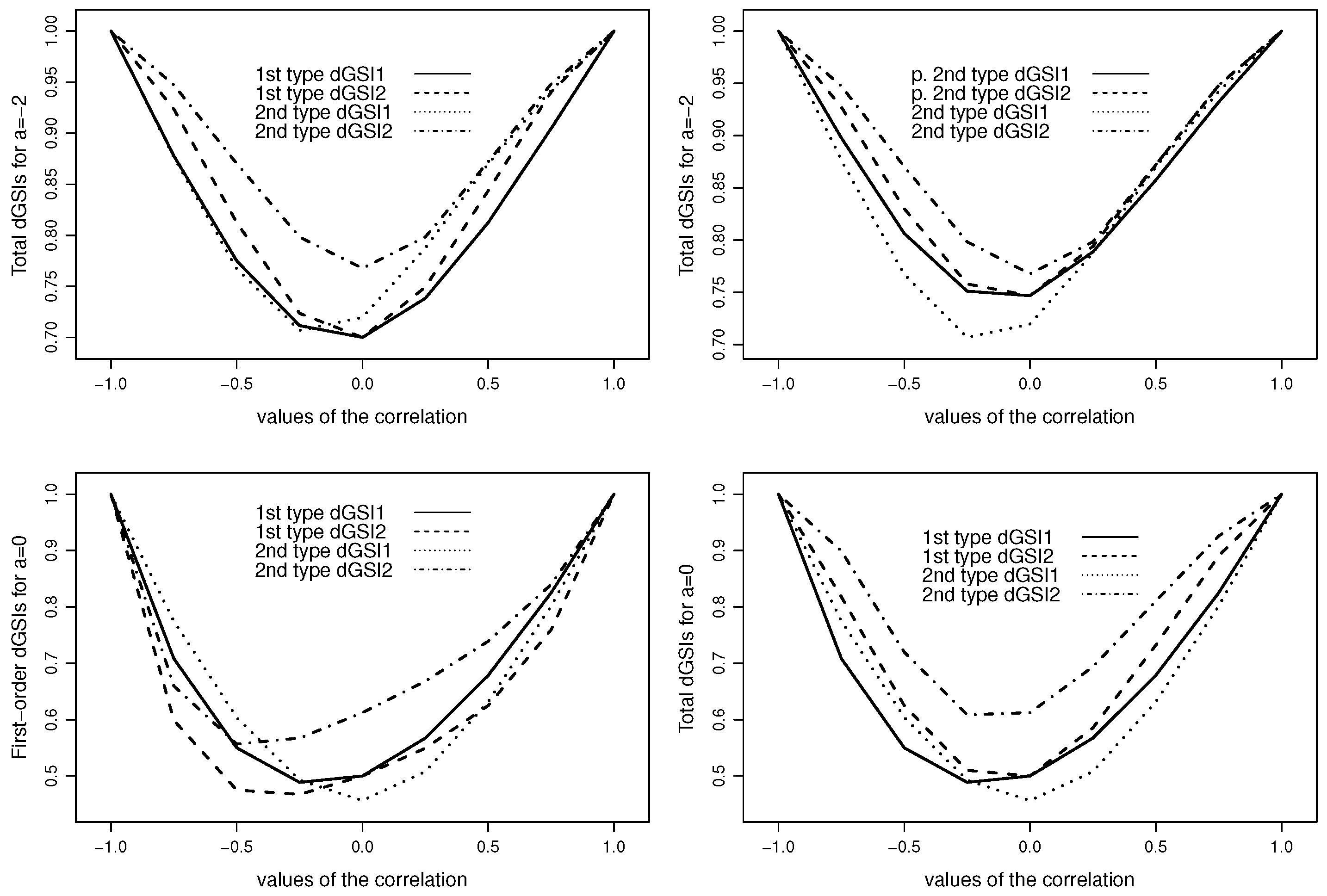
where $a\in \mathbb{R}$, $t\in [0,365]$ and $\alpha \left(t\right)\in \mathbb{R}$. When $a=0$, there is no explicit interaction between $X_1$ and $X_2$. To illustrate the difference between both types of dGSIs, we suppose that we have observed the model outputs at $t\in \{t_1,t_2\}$ with $\alpha \left(t_1\right)=1$ and $\alpha \left(t_2\right)=2$. Using the dependency functions $X_2=r_1(X_1,Z_2)=\rho X_1+\sqrt{1-{\rho }^2}{Z}_2$ and $X_1=r_2(X_2,Z_1)=\rho X_2+\sqrt{1-{\rho }^2}{Z}_1$ with $Z_i\sim \mathcal{N}\left(0,1\right)$ and $i=1,2$, Figure 1 shows the two types of dGSIs.

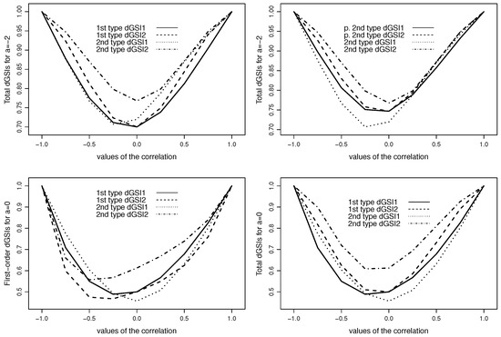
Figure 1. First-type, prime second-type, and second-type dGSIs for different values of the correlation between the two inputs and for $a=-2,0$.

The first figure (top-left panel) depicts the first-type and second-type dGSIs, and we see that both types of dGSIs give the same ranking of inputs for negative values of the correlation. In the absence of correlation (i.e., $\rho =0$), $X_1$ and $X_2$ have the same effect according to the first-type dGSIs, while the second-type dGSIs identify $X_2$ as the most influential input. When $\rho >0.5$, the first-type dGSIs show that $X_2$ is the most important input, while the second-type dGSIs suggest that both inputs have the same total effects. The second figure (top-right panel) compares the prime second-type and the second-type total dGSIs, and the results are similar to those of the first figure. The third figure (bottom-left panel) compares the first-order dGSIs of the first and second types, and it comes out that such dGSIs give different main effects of inputs for positive correlations. In the last figure, the first-type and second-type dGSIs give the same ranking of inputs except for $\rho =0$. As different rankings of inputs can happen using both types of dGSIs, and knowing that the second-type dGSIs account for the correlations among SFs, we should prefer such indices.

6.3. Sobol’s g-Function ($d=10$, $K=3$)

Here, we consider $f\left(\mathbf{x}\right):={\prod }_{j=1}^{d=10}{\displaystyle \frac{|4x_j-2|+a_j}{1+a_j}}$ with $\mathbf{a}:=(35,35,\dots ,35)\in {\mathbb{R}}^d$. The $d=10$ inputs are organized into $K=3$ blocks as follows:

• $(X_j\sim \mathcal{U}(0,1),j=4,\dots ,8)$ are independent variables, that is, ${\mathit{\pi }}_1=\{4,\dots ,8\}$;
• ${\mathit{\pi }}_2=\{1,\dots ,3\}$ and $(X_1,X_2,X_3)$ have a Gaussian copula with ${\rho }_{12}=0, {\rho }_{13}=0.01, {\rho }_{23}=0.85$ as the correlation values, and $X_j\sim \mathcal{U}(0,1),j=1,2,3$;
• ${\mathit{\pi }}_3=\{9,10\}$, where $X_9\sim \mathcal{U}(0,1),X_{10}\sim \mathcal{U}(0,1)$ with $X_9+X_{10}\le 1$.

The dependency functions of ${\mathbf{X}}_{{\mathit{\pi }}_3}$ are given by $X_{10}^c=U_{10}(1-X_9^c)$ and $X_9^c=U_9(1-X_{10}^c)$ where $U_{10}\sim \mathcal{U}(0,1)$, $U_9\sim \mathcal{U}(0,1)$; and $U_9,U_{10}$ are independent of $X_9^c\sim Beta(1,2)$, $X_{10}^c\sim Beta(1,2)$ [20].

Based on the $R_{min}=6$ ERs of $f\left(\mathbf{X}\right)$ (see Appendix J), we computed the dSIs using Sobol’s sequences and the sample size m = 10,000 (see Table 1). We can see that $X_2,X_3,X_9,X_{10}$ are the most influential inputs. For fixing $X_1$, we need the copula-based dependency model of ${\mathbf{X}}_{{\mathit{\pi }}_2}$, that is, $X_1=r_1(X_2,Z_3,Z_1)$. Since the block of inputs ${\mathbf{X}}_{{\mathit{\pi }}_1}$ is not important, we have also computed the dSIs of the pairs of variables selected out of $({\mathbf{X}}_{{\mathit{\pi }}_2},{\mathbf{X}}_{{\mathit{\pi }}_3})$ (see Table 1). As expected, the total indices are always greater than the first-order indices.

Table 1. Estimates of dSIs for Sobol’s g-function with NIVs.

	$\widehat{\mathbf{dSI}}$			$\widehat{\mathbf{dSI}}$
	Main	Total			First-Order	Total
X1	0.089	0.090		X1:X2	0.321	0.372
X2	0.241	0.294		X1:X3	0.321	0.372
X3	0.231	0.282		X1:X9	0.192	0.216
X4	0.093	0.093		X1:X10	0.193	0.217
X5	0.093	0.093		X2:X3	0.298	0.299
X6	0.093	0.093		X2:X9	0.349	0.426
X7	0.093	0.093		X2:X10	0.348	0.425
X8	0.093	0.093		X3:X9	0.334	0.407
X9	0.107	0.131		X3:X10	0.335	0.409
X10	0.108	0.132		X9:X10	0.185	0.185

7. Conclusions

In this paper, we have proposed a new way of deriving the distributions of the model outputs conditional on every subset of inputs using dependency models of random vectors of NIVs. We have provided additional generic dependency models, including empirical or computational dependency functions, of d-dimensional random vectors following many distributions, such as copula-based distributions with discrete variables, as well as distributions of inputs of complex mathematical models subjected to constraints. It came out that ${\prod }_{k=2}^K\left(\genfrac{}{}{0pt}{}{d_k}{j_{0,k}}\right)$ different equivalent representations of the model output of interest are necessary and sufficient for recovering all the conditional distributions and for assessing the effects of every subset of NIVs, including their interactions. An algorithm is then provided for selecting such representations or equivalently such dependency models.

Based on such conditional distributions and using variance–covariance as an important measure, we have extended i) dGSIs for the multivariate and/or functional outputs (including spatiotemporal models and dynamic models), and ii) dependent sensitivity indices for single-response models so as to cope with every subset of NIVs. Such indices are also well suited for models with both discrete and continuous variables. Consistent estimators of such indices and their asymptotic distributions are provided. It is worth noting that such conditional distributions are also relevant for commuting the variance-based Shapley effects [47].

Analytical test cases confirmed that the first-order index of any subset of inputs is less than its total index, as expected. In the case of the dynamic model considered, it came out that the second-type dGSIs, which account for the correlations among the components of sensitivity functionals, and the first-type dGSIs can give different rankings of input variables. Therefore, we should prefer the second-type dGSIs in practice. Moreover, it came out that the sum of the main and interaction indices can be greater than one. In the next works, it will be interesting to investigate a new approach for which the main and interactions indices sum up to one. Also, the derivation of MSEs of the estimators of covariances of sensitivity functionals is quite interesting.

Since the computations of the effects of all the subsets of inputs rely on $2^{\frac{d-d_1}{2}}\le R_{min}{2}^{d-d_1}$ ERs, which grow exponentially with respect to $d(1-\alpha )$, it becomes difficult to deploy such efficient approaches in higher dimensions under the following conditions: $\alpha =d_1/d\ll 1$ and all the K groups of NIVs are important, which is not often the case.

References

- Sobol, I.M. Sensitivity analysis for non-linear mathematical models. Math. Model. Comput. Exp. 1993, 1, 407–414. [Google Scholar]
- Lamboni, M. Multivariate sensitivity analysis: Minimum variance unbiased estimators of the first-order and total-effect covariance matrices. Reliab. Eng. Syst. Saf. 2019, 187, 67–92. [Google Scholar] [CrossRef]
- Lamboni, M.; Monod, H.; Makowski, D. Multivariate sensitivity analysis to measure global contribution of input factors in dynamic models. Reliab. Eng. Syst. Saf. 2011, 96, 450–459. [Google Scholar] [CrossRef]
- Gamboa, F.; Janon, A.; Klein, T.; Lagnoux, A. Sensitivity indices for multivariate outputs. Comptes Rendus Math. 2013, 351, 307–310. [Google Scholar] [CrossRef]
- Xiao, S.; Lu, Z.; Xu, L. Multivariate sensitivity analysis based on the direction of eigen space through principal component analysis. Reliab. Eng. Syst. Saf. 2017, 165, 1–10. [Google Scholar] [CrossRef]
- Lamboni, M. Derivative-based generalized sensitivity indices and Sobol’ indices. Math. Comput. Simul. 2020, 170, 236–256. [Google Scholar] [CrossRef]
- Perrin, T.; Roustant, O.; Rohmer, J.; Alata, O.; Naulin, J.; Idier, D.; Pedreros, R.; Moncoulon, D.; Tinard, P. Functional principal component analysis for global sensitivity analysis of model with spatial output. Reliab. Eng. Syst. Saf. 2021, 211, 107522. [Google Scholar] [CrossRef]
- Veiga, S.D.; Wahl, F.; Gamboa, F. Local Polynomial Estimation for Sensitivity Analysis on Models With Correlated Inputs. Technometrics 2009, 51, 452–463. [Google Scholar] [CrossRef]
- Mara, T.A.; Tarantola, S. Variance-based sensitivity indices for models with dependent inputs. Reliab. Eng. Syst. Saf. 2012, 107, 115–121. [Google Scholar] [CrossRef]
- Kucherenko, S.; Tarantola, S.; Annoni, P. Estimation of global sensitivity indices for models with dependent variables. Comput. Phys. Commun. 2012, 183, 937–946. [Google Scholar] [CrossRef]
- Hao, W.; Zhenzhou, L.; Wei, P. Uncertainty importance measure for models with correlated normal variables. Reliab. Eng. Syst. Saf. 2013, 112, 48–58. [Google Scholar] [CrossRef]
- Chastaing, G.; Gamboa, F.; Prieur, C. Generalized Hoeffding-Sobol’ decomposition for dependent variables—Applications to sensitivity analysis. Electron. J. Stat. 2012, 6, 2420–2448. [Google Scholar] [CrossRef]
- Kucherenko, S.; Klymenko, O.; Shah, N. Sobol’ indices for problems defined in non-rectangular domains. Reliab. Eng. Syst. Saf. 2017, 167, 218–231. [Google Scholar] [CrossRef]
- Mara, T.A.; Tarantola, S.; Annoni, P. Non-parametric methods for global sensitivity analysis of model output with dependent inputs. Environ. Model. Softw. 2015, 72, 173–183. [Google Scholar] [CrossRef]
- Tarantola, S.; Mara, T.A. Variance-based sensitivity indices of computer models with dependent inputs: The fourier amplitude sensitivity test. Int. J. Uncertain. Quantif. 2017, 7, 511–523. [Google Scholar] [CrossRef]
- Lamboni, M.; Kucherenko, S. Multivariate sensitivity analysis and derivative-based global sensitivity measures with dependent variables. Reliab. Eng. Syst. Saf. 2021, 212, 107519. [Google Scholar] [CrossRef]
- Lamboni, M. On exact distribution for multivariate weighted distributions and classification. Methodol. Comput. Appl. Probab. 2023, 25, 1–41. [Google Scholar] [CrossRef]
- Lamboni, M. Kernel-based Measures of Association Between Inputs and Outputs Using ANOVA. Sankhya A 2024, 86, 790–826. [Google Scholar] [CrossRef]
- Skorohod, A.V. On a representation of random variables. Theory Probab. Appl. 1976, 21, 645–648. [Google Scholar]
- Lamboni, M. Efficient dependency models: Simulating dependent random variables. Math. Comput. Simul. 2021, 200, 199–217. [Google Scholar] [CrossRef]
- Ferguson, T. Mathematical Statistics: A Decision Theoretic Approach; Academic Press: New York, NY, USA, 1967. [Google Scholar]
- Rschendorf, L. Stochastically ordered distributions and monotonicity of the oc-function of sequential probability ratio tests. Ser. Stat. 1981, 12, 327–338. [Google Scholar] [CrossRef]
- Rschendorf, L. Stochastic ordering of risks, influence of dependence and a.s. constructions. In Advances on Models, Characterizations and Applications; Balakrishnan, N., Bairamov, I.G., Gebizlioglu, O.L., Eds.; CRC Press: Boca Raton, FL, USA, 2005. [Google Scholar]
- Rschendorf, L. On the distributional transform, Sklar’s theorem, and the empirical copula process. J. Stat. Plan. Inference 2009, 139, 3921–3927. [Google Scholar] [CrossRef]
- Rosenblatt, M. Remarks on a Multivariate Transformation. Ann. Math. Statist. 1952, 23, 470–472. [Google Scholar] [CrossRef]
- Nelsen, R. An Introduction to Copulas; Springer: New York, NY, USA, 2006. [Google Scholar]
- McNeil, A.J.; Frey, R.; Embrechts, P. Quantitative Risk Management; Princeton University Press: Princeton, NJ, USA; Oxford, UK, 2015. [Google Scholar]
- Rosenblatt, M. Remarks on some nonparametric estimates of a density function. Ann. Math. Stat. 1956, 27, 832–837. [Google Scholar] [CrossRef]
- Parzen, E. On estimation of a probability density function and mode. Ann. Math. Stat. 1962, 33, 1065–1076. [Google Scholar] [CrossRef]
- Epanechnikov, V. Nonparametric estimation of a multidimensional probability density. Theory Probab. Appl. 1969, 14, 153–158. [Google Scholar] [CrossRef]
- Silverman, B. Density Estimation for Statistics and Data Analysis; Chapman & Hall: New York, NY, USA, 1986. [Google Scholar]
- Clayton, D.G. A Model for Association in Bivariate Life Tables and Its Application in Epidemiological Studies of Familial Tendency in Chronic Disease Incidence. Biometrika 1978, 65, 141–151. [Google Scholar] [CrossRef]
- Joe, H. Multivariate Models and Dependence Concepts; Chapman & Hall/CRC: Boca Raton, FL, USA; London, UK; New York, NY, USA, 1997. [Google Scholar]
- Smith, M.; Min, A.; Almeida, C.; Czado, C. Modeling Longitudinal Data Using a Pair-Copula Decomposition of Serial Dependence. J. Am. Stat. Assoc. 2010, 105, 1467–1479. [Google Scholar] [CrossRef]
- Durante, F.; Sempi, C. Principles of Copula Theory; CRC/Chapman & Hall: London, UK, 2015. [Google Scholar]
- Koenker, R.; Bassett, G. Regression quantiles. Econometrica 1978, 46, 33–50. [Google Scholar] [CrossRef]
- Truong, Y.K. Asymptotic Properties of Kernel Estimators Based on Local Medians. Ann. Stat. 1989, 17, 606–617. [Google Scholar] [CrossRef]
- Hendricks, W.; Koenker, R. Hierarchical Spline Models for Conditional Quantiles and the Demand for Electricity. J. Am. Stat. Assoc. 1992, 87, 58–68. [Google Scholar] [CrossRef]
- Koenker, R.; Ng, P.; Portnoy, S. Quantile smoothing splines. Biometrika 1994, 81, 673–680. [Google Scholar] [CrossRef]
- Koenker, R.; Hallock, K.F. Quantile Regression. J. Econ. Perspect. 2001, 15, 143–156. [Google Scholar] [CrossRef]
- Bassett, R., Jr.; Koenker, R. An Empirical Quantile Function for Linear Models with iid Errors. J. Am. Stat. Assoc. 1982, 77, 407–415. [Google Scholar]
- Koenker, R. Quantile Regression; Cambridge University Press: Cambridge, UK, 2005. [Google Scholar]
- Takeuchi, I.; Le, Q.V.; Sears, T.D.; Smola, A.J. Nonparametric Quantile Estimation. J. Mach. Learn. Res. 2006, 7, 1231–1264. [Google Scholar]
- Lamboni, M. Uncertainty quantification: A minimum variance unbiased (joint) estimator of the non-normalized Sobol’ indices. Stat. Pap. 2018, 61, 1939–1970. [Google Scholar] [CrossRef]
- Lamboni, M. Weak derivative-based expansion of functions: ANOVA and some inequalities. Math. Comput. Simul. 2022, 194, 691–718. [Google Scholar] [CrossRef]
- Lamboni, M. Global sensitivity analysis: An efficient numerical method for approximating the total sensitivity index. Int. J. Uncertain. Quantif. 2016, 6, 1–17. [Google Scholar] [CrossRef]
- Owen, A.B. Sobol’ Indices and Shapley Value. Siam/Asa J. Uncertain. Quantif. 2014, 2, 245–251. [Google Scholar] [CrossRef]
- Sugiura, N. Multisample and multivariate nonparametric tests based on U-statistics and their asymptotic efficiencies. Osaka J. Math. 1965, 2, 385–426. [Google Scholar]
Disclaimer/Publisher’s Note: The statements, opinions and data contained in all publications are solely those of the individual author(s) and contributor(s) and not of MDPI and/or the editor(s). MDPI and/or the editor(s) disclaim responsibility for any injury to people or property resulting from any ideas, methods, instructions or products referred to in the content. |
© 2025 by the author. Licensee MDPI, Basel, Switzerland. This article is an open access article distributed under the terms and conditions of the Creative Commons Attribution (CC BY) license (https://creativecommons.org/licenses/by/4.0/).