Abstract
Optimization techniques aim to identify optimal solutions for a given problem.
In single-objective optimization, the best solution corresponds to the one that maximizes or
minimizes the objective function. However, when dealing with multi-objective optimization,
particularly when the objectives are conflicting, identifying the best solution becomes
significantly more complex. In such cases, exact or analytical methods are often impractical,
leading to the widespread use of heuristic and metaheuristic approaches to identify
optimal or near-optimal solutions. Recent advancements have led to the development
of various nature-inspired metaheuristics designed to address these challenges. Among
these, the Whale Optimization Algorithm (WOA) has garnered significant attention. An
adapted version of the WOA has been proposed to handle multi-objective optimization
problems. This work extends the WOA to tackle multi-objective optimization by incorporating
a decomposition-based approach with a cooperative mechanism to approximate
Pareto-optimal solutions. The multi-objective problem is decomposed into a series of
scalarized subproblems, each with a well-defined neighborhood relationship. Comparative
experiments with seven state-of-the-art bio-inspired optimization methods demonstrate
that the proposed decomposition-based multi-objective WOA consistently outperforms its
counterparts in both real-world applications and widely used benchmark test problems.
Keywords:
multi-objective evolutionary optimization; decomposition-based optimization; whale optimization algorithm MSC:
68T20
1. Introduction
Optimization problems are prevalent across various industries, involving the search for optimal values of decision variables to achieve the best solution. However, exact methods often need to be more practical, necessitating metaheuristics. Numerous real-world problems also require the simultaneous optimization of several competing objectives. Such problems are referred to in the literature as multi-objective optimization problems (MOPs). Finding decision variable values that offer the optimum trade-offs between many objectives is the goal of multi-objective optimization, which makes the optimization work more difficult.
Several metaheuristic algorithms that draw inspiration from natural processes have been created recently. These methods are often categorized by the paradigm from which they draw inspiration, with one prominent paradigm being swarm intelligence. These approaches explore the collective behaviors that arise from interactions between individual components and their environment. Several notable metaheuristics have emerged within the swarm intelligence paradigm, including Particle Swarm Optimization [1], Ant Colony Optimization [2], the Artificial Bee Colony [3], the Gray Wolf Optimizer [4], and the Whale Optimization Algorithm [5], among others. These algorithms harness collective intelligence principles to tackle optimization challenges.
The social behavior of whales, especially humpback whales’ hunting tactics, served as the inspiration for the Whale Optimization Algorithm (WOA), a metaheuristic. It employs concepts of exploration and exploitation to find optimal solutions. Throughout the search phase, the algorithm explores the solution space by strategically updating the whales’ positions, allowing for diverse exploration.
By moving the whales’ locations in the direction of the best solution thus far discovered, the algorithm converges towards promising areas of the solution space throughout the encircling phase. The WOA applies a randomization element based on the bubble-net feeding behavior to prevent local optima while promoting comprehensive exploration of the solution space. Conventional optimization algorithms such as the WOA focus on finding a single optimal solution, but real-world scenarios often require optimizing multiple conflicting objectives simultaneously.
Recent research has introduced extensions to the WOA to tackle MOPs [6,7,8,9]. One such extension, the Non-Dominated Sorting Whale Optimization Algorithm (NSWOA) [9], uses the Pareto dominance principle to address MOPs. The NSWOA applies a non-dominated sorting strategy that categorizes solutions into different levels or fronts. Solutions that are not dominated by any other belong to the first front. The algorithm assigns a fitness value to each solution based on its front and the agglomeration distance between neighboring solutions. A key limitation of Pareto-based Multi-Objective Evolutionary Algorithms (MOEAs), such as the NSWOA, is their decreasing effectiveness as the number of objectives increases. While the NSWOA has demonstrated competitive performance compared to other algorithms, there is still room for improvement in multi-objective optimization. Historically, multi-objective algorithms have relied on Pareto-based and performance indicator-based approaches. However, these methods face challenges: Pareto-based MOEAs struggle as the number of objectives grows, while indicator-based MOEAs increase computational costs. Decomposition-based approaches, which bio-inspired metaheuristics have not fully explored, offer a promising alternative. This has led to the development of new decomposition-based strategies for addressing complex MOPs in real-world applications, which is the primary focus of the present investigation.
This paper presents a novel multi-objective algorithm based on the WOA that uses swarm intelligence approaches to avoid the drawbacks of current multi-objective algorithms. The algorithm has several key features, including the following:
- The decomposition of multi-objective problems: the suggested algorithm improves the approximation of Pareto optimum solutions by separating complex multi-objective issues into scalarizing subproblems.
- Divide and conquer strategy: the proposed approach defines a neighborhood link between subproblems and whales, which can strategically move and collaborate to address nearby subproblems.
- No external archive: this method eliminates the need for extra processing time because it does not involve an external archive, contrary to many bio-inspired multi-objective systems.
Multi-objective optimization problems in continuous and unconstrained domains can be solved using the suggested method. Experiments are carried out utilizing two real-world applications with unknown features and a well-known test suite to assess their performance. According to the results of our comparison investigation, the suggested method is computationally efficient and performs more effectively than seven cutting-edge algorithms.
The structure of the paper is as follows. Section 2 introduces the principles of evolutionary multi-objective optimization, while Section 3 reviews related research. Section 4 describes the proposed decomposition-based multi-objective algorithm. The experimental study is presented in Section 5, followed by an analysis of two real-world applications in Section 6. Finally, Section 7 provides conclusions and describes potential paths for future investigation.
2. Multi-Objective Evolutionary Optimization
This section begins with an introduction to the fundamental concepts related to multi-objective optimization, followed by a description of the three evolutionary methodologies for addressing problems with multiple objectives. Finally, the section concludes with a description of the decomposition approach for multi-objective optimization problems.
2.1. Multi-Objective Optimization in a Nutshell
Consider a continuous minimization problem. The formulation of a multi-objective optimization problem (MOP) is given by (without loss of generality, we assume minimization problems since [10]):
such that , F is the vector of the M objective functions, and, regarding that represents the decision variable space,
Here, () are the functions to be optimized. For box-constrained problems, which are the focus of this study, , meaning for all .
In single-objective optimization, the scalar objective values can be compared using the “less than or equal to” (≤) relation, which induces a total order on . Sorting solutions from best to worst is made possible by this overall order. Weaker order definitions are necessary to compare vectors in since there is no such canonical order on in multi-objective optimization problems. The following definitions are offered to handle this [11].
Definition 1.
Let . We say that dominates (denoted by ) if and only if and .
Definition 2.
Let . We say that is a Pareto optimal solution if there is no other solution such that .
Definition 3.
The Pareto set (PS) of an MOP is defined by:
Definition 4.
The Pareto front (PF) of an MOP is defined by:
The primary objective in multi-objective evolutionary optimization is to generate diverse solutions from the Pareto optimal set, ensuring that these solutions are well distributed across the Pareto optimal front.
2.2. Evolutionary Approaches for Multi-Objective Optimization
Identifying the best trade-offs between conflicting objectives is essential to solving multi-objective optimization problems. Unlike single-objective optimization, which results in a single optimal solution, this approach produces a set of solutions that represent the best compromises among various objective functions. Due to their population-based approach, multi-objective evolutionary algorithms (MOEAs) are widely used for these problems. MOEAs are typically classified into three main types: Pareto-based, indicator-based, and decomposition-based methods.
- Pareto-based approaches. The Pareto dominance relation is the most commonly used method for comparing objective vectors in multi-objective optimization. Many MOEAs rely on this technique to rank the population, evaluate proximity to the Pareto front (PF), and guide selection for mating or survival. Examples include dominance deep [12], dominance rank [13], and dominance count [14]. To enhance the distribution of solutions, Pareto dominance is often combined with methods such as fitness sharing [15], clustering [14], and crowding distance [16]. This combination is important because obtaining a good approximation of the PF requires balancing both convergence and diversity. Although Pareto-based MOEAs were widely used in the early 2000s, their popularity has decreased due to challenges in spreading solutions [17,18,19] and diminished effectiveness in high-dimensional spaces [20,21].
- Indicator-based approaches. This method in MOEAs achieves a good representation and approximation of the PF by using a performance indicator. The creation of new algorithms based on this idea was made possible by the Indicator-Based Evolutionary Algorithm (IBEA) [22]. [23], [24], and hypervolume [25] are a few examples of indicators that evaluate convergence and diversity, but they can be computationally expensive, particularly when there are numerous objectives. RIB-EMOA [26], MOMBI-II [27], and LIBEA [28,29] are a few indicator-based techniques.
- Decomposition-based approaches. Over the past decade, decomposition-based approaches, which rely on scalarizing functions, have gained prominence in MOEAs. These methods solve multiple scalarizing functions, each guided by a weight vector, to tackle multi-objective problems. A new age of MOEAs began with the introduction of the multi-objective evolutionary algorithm based on decomposition (MOEA/D) [30], which provided efficient and effective problem-solving capabilities. Various improvements and adaptations of the MOEA/D are discussed in [31,32,33]. Other decomposition-based metaheuristics include MOPSO/D [34], dMOPSO [35], and MOGWO/D [36].
Typically, evolutionary algorithms for multi-objective optimization are built upon the three multi-objective evolutionary approaches mentioned earlier. For a more detailed analysis, refer to the works [37,38,39].
2.3. The Decomposition of a Multi-Objective Problem
It is widely acknowledged that a Pareto optimal solution to the problem in Equation (1) can also be viewed as an optimal solution to a scalar optimization problem, where the objective function combines all the individual objective functions [11].
To achieve this, several scalar aggregation methods have been proposed. The scalar Tchebycheff approach [40] is considered one of the most commonly used techniques for this purpose. The Tchebycheff scalar method transforms the vector of objective function values into a single-objective scalar optimization problem. This can be expressed as follows:
Here, represents the feasible region, is a reference point where , and is a convex weight vector, with for all j and .
For each Pareto optimal point , there exists a convex weight vector such that is the optimal solution to the problem in Equation (2). On the other hand, any Pareto optimal solution of the problem in Equation (1) corresponds to an optimal solution of Equation (2).
Thus, different scalar optimization problems described by different weight vectors can be solved to obtain an effective representation of the Pareto front. During the optimization process, these weight vectors define the search direction. This concept is central to both traditional mathematical programming techniques for multi-objective problems and modern multi-objective evolutionary approaches based on decomposition.
3. Related Work
We can find many proposals to solve multi-objective optimization problems. However, the related work reviewed in this investigation is focused on related studies dealing with the Whale Optimization Algorithm (WOA), multi-objective optimization approaches based on the WOA, and bio-inspired decomposition-based approaches for multi-objective optimization.
3.1. Whale Optimization Algorithm
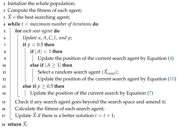
The Whale Optimization Algorithm (WOA) [5] is a metaheuristic inspired by the social behavior of humpback whales.. Key advantages of the WOA include its balanced approach to exploration and exploitation, two distinct exploitation methods, a flexible mechanism that helps avoid local optima, and minimal structural adjustments for different problems, as it only requires tuning two main parameters. The algorithm starts by generating a random population of whales, which then search for prey using the bubble-net hunting strategy, encircling their target. The key search movements of the WOA are outlined below.
- Encircling prey. Using this technique, the whale modifies its location according to the best-known location. By decreasing the distance between its present location and the best-known individual, the whale progressively approaches this ideal solution. This method aids in focusing the search on regions that show promise. The following is a description of the mathematical specifics of this position adjustment:where denotes the space between a whale and the prey position vector. The component t denotes the current iteration, represents the position vector, and refers to the position vector of the best solution found so far. and are coefficient vectors defined by:where the value of falls linearly between two and zero as iterations increase and is a random vector .
- Bubble-net attacking method. The bubble-net strategy can be implemented using two approaches: (1) the shrinking encircling mechanism and (2) spiral position updating. By decreasing the value of in Equation (5), the shrinking encircling process reduces . The spiral position update mimics the humpback whale’s spiral trajectory by imitating the whale’s movement around its target prey using a spiral equation:where l is a random number , b is a constant that establishes the shape of the logarithmic spiral, and represents the distance between the whales and their prey. · is a multiplication of elements. It is essential to remember that the humpback whale can swim both a spiral path and a shrinking circle around its food. The following is a mathematical expression of this behavior:where is a random number that represents the likelihood of selecting the spiral model or the shrinking encircling approach to fit the whales’ positions.
- Search for prey. In the exploration phase, humpback whales search for prey more broadly by exploring the solution space. A random search agent is selected instead of using the best-known search agent to guide the process. This approach helps the whales explore new regions and reduces the risk of becoming trapped in local optima. The position of each whale is updated based on this randomly chosen agent, allowing for greater diversity in the search process.where a randomly selected point from the current population is denoted by . Algorithm 1 describes the general process of the Whale Optimization Algorithm (WOA). The original article [5] is recommended to the interested reader for a comprehensive explanation and detailed approach.
| Algorithm 1: General framework of WOA [5] |
 |
3.2. Multi-Objective Approaches Based on the WOA
In specialized research, several notable contributions focus on multi-objective optimization using the Whale Optimization Algorithm (WOA). One significant extension is the multi-objective version of the WOA (MOWOA), proposed by Dao et al. [6], which applies the algorithm to the robot route planning problem. In this case, two criteria, distance and path smoothness, are transformed into a minimization problem. Another example by Kumawat et al. [8] demonstrates that this multi-objective variant of the WOA not only shows accurate convergence on the Pareto front but also maintains effective diversity among solutions while preserving the benefits of the original WOA.
Additionally, Kasturi and Nayak [41] present an interesting application where a novel MOWOA technique is used to identify optimal locations for Electric Vehicle (EV) charging stations, considering solar (PV) and battery energy storage (BES). Another notable proposal is by El Aziz et al. [42], who adapt the WOA algorithm for multi-level thresholding in image segmentation, using objective functions such as Otsu inter-class variance maximization and Kapur entropy.
Another remarkable use of the WOA algorithm in a multi-objective context is by Narendrababu Reddy and Kumar [43], who apply it in cloud computing environments. Their approach optimizes energy, quality of service, and resource utilization. An interesting version of the MOWOA is also developed in [44], where it is tested on several well-known benchmark problems, utilizing performance indicators like inverted generational distance (IGD) for comparison.
In another study, Shayeghi et al. [45] combine the MOWOA with a fuzzy decision-making system to optimize the location and size of Distributed Flexible AC Transmission System (D-FACTS) devices and Unified Power Quality Conditioners (UPQCs). A unique non-dominated sorting algorithm based on multi-objective whale optimization for content-based image retrieval (NSMOWOA) was introduced in [7], offering an intriguing method for this domain.
Further interesting studies include [46], which combines the Opposition-Based Learning approach with the WOA, employing a Global Grid Ranking (GGR) system. To reduce energy consumption and extend the lifespan of large-scale wireless sensor networks (LSWSNs), Ahmed et al. [47] propose using the MOWOA to determine the minimum number of receiver nodes required to cover the network.
Saleh et al. [48] extend the MOWOA with three objective functions to optimize the distributed generation (DG) and capacitors in radial distribution systems, which is a compelling implementation. Additionally, in [49], the NSWOA is applied to a hydro–photovoltaic (PV)–wind energy system model, where the goal is to maximize yearly power generation while minimizing power variability. These are just a few examples of how the multi-objective variant of the WOA algorithm has been applied in various domains.
3.3. Bio-Inspired Decomposition-Based Approaches for Multi-Objective Optimization
One of the earliest examples of MOEAs using decomposition intrinsically is given in the literature by Ishibuchi et al. [50]. Their algorithm, Multi-Objective Genetic Local Search (MOGLS), showed a different way of solving MOPs following evolutionary computation principles and scalarizing functions. However, significant progress in decomposition-based approaches was made in the 2000s with the development of the Multi-Objective Evolutionary Algorithm based on Decomposition (MOEA/D) [30]. To reduce computational complexity, the MOEA/D introduced the idea of breaking down an MOP into many scalar optimization subproblems and optimizing them concurrently. This approach marked the beginning of more efficient methods for solving MOPs. Several extensions of the MOEA/D were later developed, including those by Li et al. [31] and Zhang et al. [51]. These research efforts provide the groundwork for a wide range of decomposition-based evolutionary algorithms for multi-objective optimization.
In addition to evolutionary algorithms, swarm intelligence methods have also been used to solve multi-objective optimization issues through decomposition. One of the first such approaches was the Multi-Objective Particle Swarm Optimizer based on Decomposition (MOPSO/D) [34]. This method integrates the decomposition strategy from the MOEA/D, where the MOP is transformed into a set of scalar aggregation subproblems. Each scalar problem function has a particle in the swarm, with weights established for each objective function. A notable extension of this approach is the decomposition-based Multi-Objective Particle Swarm Optimizer (dMOPSO) [35], which updates particle positions using the best solutions derived through decomposition techniques. Other PSO-based methods have been proposed to improve performance, including those investigations reported in [52,53,54]. Beyond PSO, the Multi-Objective Artificial Bee Colony Algorithm based on Decomposition (MOABC/D) [55] applies decomposition to swarm intelligence, using artificial bee colonies [56,57] to approximate Pareto optimal solutions. Similarly, the Multi-Objective Teaching–Learning Algorithm based on Decomposition (MOTLA/D) [58] builds on the teaching–learning strategy developed by Rao et al. [59] to optimize MOPs using decomposition. More recently, the Decomposition-based Multi-Objective Symbiotic Organism Search (MOSOS/D) algorithm [60] was introduced. This method is based on the symbiotic interactions among organisms and is capable of solving large and complex MOPs. The Cuckoo Search (CS) algorithm for multi-objective problems with a decomposition approach [61] is another noteworthy contribution. It selects from a pool of operators using an adaptive operator selection mechanism based on bandits.
The Ant Colony Optimizer (ACO) was also adapted for multi-objective optimization using decomposition. Ning et al. [62] proposed the Negative Pheromone Matrix-based ACO (NMOACO/D), which maintains both positive and negative pheromone matrices to update non-dominated solutions. Zhao et al. [63] developed the MaOACO/D-RP algorithm, which incorporates an adaptive set point mechanism to optimize set points based on the distribution of solutions throughout the iterative process. A decomposition-based approach has also been explored in the domain of immune algorithms. Li et al. [64] proposed a variant of multi-objective immune algorithms (MOIAs) called the MOIA with a Decomposition-based Clonal Selection Strategy (MOIA-DCSS). This method enhances diversity in the population of solutions and employs differential evolution to increase the algorithm’s exploration abilities.
The suggested algorithm based on the WOA, which considers the decomposition principle for multi-objective optimization, is described in depth in the following section.
4. Decomposition-Based Multi-Objective Whale Optimization
The proposed Multi-objective Whale Optimization Algorithm based on decomposition (MOWOA/D), presented in this research, tackles MOPs by decomposing them down into a number of single-objective subproblems. This method gives a more precise approximation of the PF by solving a set of N scalar subproblems, each of which is derived from the original MOP. The MOWOA/D uses the appropriate weight vector and scalar function for each subproblem to find the best solution during the search phase.
As with other MOEAs based on decomposition, the MOWOA/D is an a posteriori algorithm, meaning it achieves a sample of the whole PF. These alternative solutions are then presented to the decision maker, who can choose the preferred solution(s) based on specific requirements. Unlike a posteriori weighting methods, decomposition-based approaches differ in their handling of scalar single-objective problems. Each problem is addressed independently in weighting methods, often requiring multiple executions of an optimization algorithm. In decomposition-based approaches, however, all subproblems are solved simultaneously, with individuals in the population contributing to the optimization of any subproblem.
Several methods exist for decomposing problems to approximate Pareto optimal solutions, but boundary intersection-based methods offer distinct advantages over alternatives like the Tchebycheff and weighted sum approaches (for further discussion, see [30,65]). Therefore, the MOWOA/D uses the Penalty Boundary Intersection (PBI) method [30] as its decomposition approach. Formally, the scalar optimization problem described by the PBI approach [30] consists in minimizing:
For example:
where , such that , is the set of feasible solutions, and is a weight vector such that and for each .
Due to the nature of general multi-objective optimization problems, the vector is unknown. Therefore, the proposed MOWOA/D assigns each component the minimum value found for each objective () along the search process.
When the process first starts, there are N whales in the population , initialized randomly. Each whale is tasked with optimizing the i-th subproblem defined by a weight vector , drawn from a well-distributed set of N weight vectors . Consequently, each whale optimizes its associated scalarized problem for moving into a better location to pursue its prey. Different from existing multi-objective approaches based on the WOA, the MOWOA/D performs the hunting process cooperatively. For each whale , let be the neighborhood of the T closest weight vectors to within . For convenience, only contains the indices of the T closest weight vectors to . Similarly, let be the complement set of indices. In this manner, a sub-group of whales, s (), is implicitly specified to cooperatively optimize the i-th subproblem (), which is determined by the weight vector . The position update process in the MOWOA/D works as follows. The first step is to update the values of a, p, l, A, and C. In contrast to the original WOA, the MOWOA/D employs a probability (provided by the user) to decide whether to use the bubble-net attack approach or the encircling prey/search for prey phase.
If , the encircling prey phase is applied according to Equation (4), with and , where is a random index selected from . Otherwise, the search for prey phase is performed, following Equation (10), where and , where is a random index chosen from . The encircling prey movement implicitly carries out the exploitation phase, while the search for prey movement carries out exploration. As a result, the best positions in the population are updated accordingly. In the MOWOA/D, when the encircling prey (exploitation) is performed, the neighborhood to be updated is local, i.e., . On the other hand, during the search for prey (exploration) phase, the complement of is updated, i.e., .
If , the bubble-net attack method is performed according to Equation (7), with and , where is a random index selected from . In this case, the neighborhood to be updated is stated as .
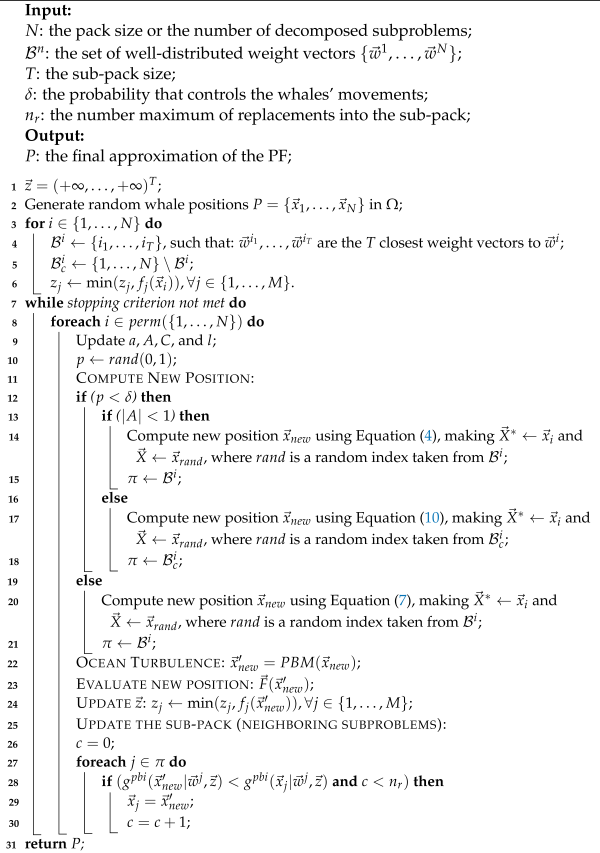
The MOWOA/D integrates an ocean turbulence mechanism applied after determining the new whale position (). To simulate this, the MOWOA/D uses the PBM operator [16], resulting in the updated position (), which is then evaluated. After evaluation, the reference point is updated. Finally, if is better than the whale positions in the neighborhood , those positions are replaced. To maintain diversity, the number of replacements in is limited to a maximum of . The steps of the hypothesized MOWOA/D are described in Algorithm 2.
| Algorithm 2: A general framework of the proposed MOWOA/D |
 |
5. Experimental Study
In the experimental study, the main goal is to evaluate the performance of the proposed MOWOA/D on both benchmark test functions and real-world scenarios. To achieve this, this section first introduces the baseline algorithms for comparison with the MOWOA/D, followed by a description of the experimental setup, which details the configuration of each algorithm used in the study. Next, the multi-objective performance indicators employed in this study are presented. The two parameters of the MOWOA/D are then tuned to determine the values that yield optimal performance. Finally, the solutions obtained by the MOWOA/D are compared with those generated by the baseline algorithms to assess overall performance.
5.1. Adopted Algorithms for Performance Comparison
As mentioned earlier, the literature includes numerous metaheuristic algorithms designed for solving multi-objective problems. In this study, six modern algorithms have been selected to compare the performance of the proposed MOWOA/D, as their methodologies align with the objectives of this investigation.
More specifically, the algorithms that have been selected to be compared in this investigation are the NSWOA [9], MO-SCA [66], MOEA/D [30], MOPSO/D [34], MOTLA/D [58], and MOABC/D [55]. All of these algorithms were adapted in accordance with their standard parameters and in order to achieve optimal performance in alignment with the specifications outlined in their original articles.
5.2. Experimental Setup
The solutions found by the MOWOA/D were validated against those reached by the NSWOA, MO-SCA, MOEA/D, MOPSO/D, MOTLA/D, and MOABC/D on the UF benchmark test suit [67]. To guarantee a fair comparison, the population size N was the same for all algorithms. The number of subproblems that the algorithms were able to deconstruct naturally expressed this value. Using a well-distributed collection of weight vectors and a penalty value of , the PBI method was used to define the scalar subproblems. As employed by Zhang et al. [30], the normalized PBI method was used to handle different objective scales. The simplex-lattice design [68] was used to define the weight vectors. Consequently, , where M is the number of objectives, corresponds to the number of weight vectors. Thus, the number of weights N is controlled by the parameter H. The weight vectors in this study are 100, 210, 220, and 210, respectively, since when , when , when , and when .
For each decomposition-based MOEA, the search was limited to performing fitness function evaluations for UF test problems and for real-world problems. The remaining parameters were defined as follows:
- NSWOA: It was configured using standard values according to its authors: l was set to randomly select a value in the interval , and .
- MO-SCA: It was set to use the parameter values proposed by the authors: , where , which means that linearly decreases from a to 2, , , and . Function returns a random value from the interval . g is the current iteration, and is the maximum number of generations.
- MOEA/D: It was executed employing the parameters recommended by its authors. That is, , , , , and , where n denotes the number of decision variables.
- MOPSO/D: It was set considering the suggestions accustomed by its authors. More precisely, , , , , and . The velocity constraints () and the inertia factor (w) were set as recommended in [69,70]. More precisely, these values were uniformly distributed for each velocity calculation in the ranges and .
- MOABC/D: It was executed following the suggestions stated by its authors. , , , , and .
- MOTLA/D: It was configured according to the suggestions proposed by its authors. , , and , where n denotes the number of decision variables.
- MOWOA/D: It was performed using and . The parameters’ sub-pack size () and probability threshold () were analyzed. The outcomes of this parameter study are conferred later in this section, suggesting for this approach and . The parameters for the ocean turbulence were set as and , where n is the number of decision variables.
In addition, a table of the parameters used is presented for better visualization (Table 1). It is also noteworthy that the parameters of the algorithms used for the comparison were obtained from the original articles and subsequently adapted to the requirements of the experimental tests.

Table 1.
Parameter settings of experiments.
5.3. Performance Assessment
MOEAs have garnered significant attention from the research community. With the increasing interest in developing new approaches and proposals, numerous performance indicators have been introduced to enhance the quality of comparisons [71,72]. For multi-objective problems, the outcome is typically an approximation of the Pareto front, focusing on the closeness and distribution of the solutions. Given that the analysis of the Pareto approximation has primarily been empirical, evaluating and comparing the performance of different multi-objective methods has become a crucial area of study. To enable more quantitative comparisons, Ref. [73] reviewed the statistical performance of several methods based on Pareto dominance. In this context, MOEAs are assessed using two performance indicators that measure the closeness and distribution of the non-dominated solutions produced by a multi-objective technique. These indicators are described in detail below.
5.3.1. Inverted Generational Distance Plus
According to Coello and Reyes [23], the concept of generational distance was first introduced in [74,75] to estimate how far the elements of a Pareto approximation produced by an algorithm are from the true Pareto front of a given problem. Later, Ishibuchi et al. [76] proposed a modification to the inverted generational distance, called the inverted generational distance plus (). This is a weakly Pareto-compliant performance indicator that incorporates an adjustment to assess the quality of generated solutions against a larger reference set. The formulation of is as follows:
In the above equation, is the reference , is an approximation to the , and is defined as:
For this performance measure, a value closer to zero indicates that each non-dominated solution obtained by an algorithm is nearer to the Pareto front.
5.3.2. Normalized Hypervolume Indicator
The hypervolume performance indicator (), introduced by Zitzler and Thiele [25], provides a qualitative assessment of MOEA performance. It quantifies both the distribution and proximity of non-dominated solutions throughout the Pareto optimal front. The hypervolume represents the non-overlapping volume of all hypercubes formed between a user-defined reference point and each solution in the Pareto front approximation (). Mathematically, the hypervolume is expressed as follows:
From the above equation, denotes the Lebesgue measurement. represents the reference vector being dominated by all the solutions in . Using the above equation, the normalized indicator is defined as follows:
Here, is the known ideal vector and M denotes the number of objectives. A higher value of this indicator implies that the set has a better approximation and distribution over the Pareto front. The range of this indicator is .
5.4. Parameter Tuning
The performance of MOWOA/D in finding accurate Pareto front approximations largely depends on two parameters: the sub-pack size (T) and the probability threshold () for selecting the update position method. A tuning process was conducted to determine the best values for these parameters. The results to variate the T and parameters are shown in the heat map of Figure 1. This figure presents two main sets of heat maps corresponding to the two performance indicators and . For each heap map set, there are ten heap maps, one corresponding to each UF test function. Each heat map shows the sub-pack size T in the vertical axis and the probability threshold in the horizontal axis. The heat map’s darker regions represent better performance indicator values.
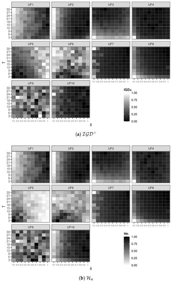
Figure 1.
A performance assessment of the MOWOA/D with varying values of parameters T and . The plots show (a) the indicator and (b) the indicator. For clarity, the values are normalized for each test problem.
From this figure, we can observe that, for test functions UF2, UF4, UF7, UF8, and UF10, values of and make the MOWOA/D find appropriate Pareto front approximations. This can be seen in the darker regions of the heat maps for both and . There is no clear evidence for the remaining test functions that any value of or T supports the MOWOA/D in obtaining proper approximation sets.
Given these observations, we can conjecture that and T would benefit the MOWOA/D if they were adjusted automatically during the execution. This particular feature of the MOWOA/D will be discussed later as part of future work. However, in the proposed MOWOA/D, the suggested values for these parameters are and .
The parameter defines the maximum number of replacements allowed for a solution within a neighborhood. This parameter has been examined in previous studies focusing on the design of MOEAs based on decomposition; see the investigations presented in [31,77]. These studies have suggested that the number of replacements should be considerably smaller than the neighborhood size being updated. In our research, we set , in line with the recommendation made by Li et al. [31].
5.5. Algorithm Performance Assessment
The proposed MOWOA/D is compared to the six multi-objective algorithms presented earlier in terms of the and performance indicators. Table 2 and Table 3 show the average performance indicator values and the corresponding standard deviation for the and , respectively.
Table 2.
Average values for each UF test function obtained by multi-objective algorithms under consideration. Bold values show the best performance and underlined values indicate that the concerned algorithm significantly outperformed all other algorithms.
Table 3.
Average values for each UF test function obtained by multi-objective algorithms under consideration. Bold values show the best performance and underlined values indicate that the concerned algorithm significantly outperformed all other algorithms.
In order to provide a more effective visualization of the results obtained by the performance indicators used for the comparison, the best average values of the results are highlighted in bold. Additionally, to provide a way to identify significant differences, it was decided to consider the non-parametric statistical Wilcoxon test [78], using a p-value of 0.05 and Bonferroni [79] correction. Therefore, if an algorithm is statistically better than others, it can be considered superior concerning the respective performance indicator. In this case, the value is underlined.
Table 2 shows the results obtained for the performance indicator for the ten benchmark functions. As we can see, the MOWOA/D was able to find approximation sets to six test functions that achieved the closest distance to the Pareto front, namely, UF1, UF2, UF3, UF8, UF9, and UF10. Moreover, the improvement is statistically significant for four of these six test functions. For the other four test functions, three different algorithms found the best non-dominated sets, with only one being statistically superior.
On the other hand, Table 3 shows the results obtained for the performance indicator for the ten benchmark functions. Again, the MOWOA/D obtained the best average hypervolume in the same six benchmark functions for the indicator, though the difference is not significantly greater. Similarly to the case, the best averages for the other four benchmark functions were obtained by the same three algorithms, and none of them was statistically significant.
In summary, we can conjecture that the MOWOA/D was the best algorithm for finding better approximation sets for six out of the ten test functions.
Additionally, to analyze the performance of the MOWOA/D in terms of the and indicators, it is important to have an idea of the Pareto approximations produced by the proposed MOWOA/D. Figure 2 depicts the approximation and distribution of the non-dominated solutions found by a typical MOWOA/D execution for each UF test problem. In these plots, it is observable that the MOWOA/D has a low performance on problems UF5 and UF6, which is consistent with the results of the and indicators. On average, it is possible to see the good performance of the proposed MOWOA/D in the majority of the UF test problems.
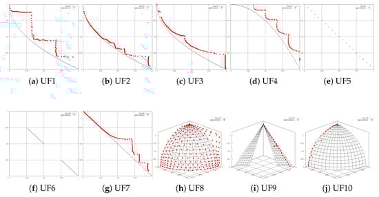
Figure 2.
Pareto front approximations obtained by MOWOA/D on UF test suite.
Considering the analysis made in the present experimental study, we find that the proposed MOWOA/D is, overall, adequate to tackle multi-objective problems that involve complicated Pareto sets.
5.6. Computational Complexity
At each iteration of the MOWOA/D, N new solutions are generated to represent the evolution of whale positions throughout the search space. These solutions update the neighborhood structure of the whales, which directly impacts the computational effort required for each iteration. Specifically, the update process of the whales’ neighborhoods (outlined in lines 27–30 of Algorithm 2) constitutes the primary computational bottleneck in the MOWOA/D.
The neighborhood update’s computational complexity is determined by the cardinality of the set , which varies probabilistically based on the parameter . In particular, the cardinality of could take a maximum value with probability and T with probability ; see lines 12–21 in Algorithm 2. This probabilistic behavior affects the number of solutions that need to be updated between whales, which in turn determines the computational complexity.
This probabilistic behavior influences how many solutions need to be updated between whales, which directly determines the computational complexity.
- Computational complexity for one whale update. The time complexity for updating a single whale’s position in one iteration of the MOWOA/D can be described as follows:
- –
- With probability : .
- –
- With probability : .
- Computational complexity for the whole pack of whales. Given N whales in the population, the overall computational complexity per iteration is as follows:
- –
- With probability : .
- –
- With probability : .
Therefore, in the worst case, the computational complexity of the MOWOA/D is:
This complexity is comparable to most of the traditional MOEAs, which also have a computational complexity of .
6. Performance on Two Real-World Applications
The MOWOA/D was also run to solve two real-world multi-objective problems. Such problems are introduced first in this section, followed by an analysis of the MOWOA/D’s performance on these two real-world applications.
6.1. Real-World Multi-Objective Problems
The two real-world multi-objective problems chosen for assessing the MOWOA/D’s performance were taken from the literature and are introduced next.
- Liquid-rocket single-element injector design.Injectors for liquid-rocket propulsion can be divided into two basic types, depending on how the propellant is mixed [80]. The first type is an impact element where mixing is achieved by direct impact of the propellant streams at an acute angle. The second injector type consists of non-impact elements in which the fuel streams flow in parallel, usually in a coaxial direction [81]. The aforementioned principles have yielded a hybrid element, as developed by The Boeing Company (U.S. Patent 6253539) [82], which is utilized in the design of a single-element liquid-rocket engine injector. The liquid-rocket single-element injector design (LSID) problem involves optimizing the injectors used in liquid-rocket engines. The consideration of these design variables is imperative when addressing the design problem of the injector. The subsequent list enumerates the design variables, their reference values, and their respective ranges:
- –
- Hydrogen flow angle ) is the angle at which hydrogen is directed toward the oxidizer. The maximum angle varies between and . The baseline hydrogen flow angle is .
- –
- Hydrogen area is defined as the incremental change in the cross-section area of the tube carrying hydrogen, relative to the baseline cross-section area of . This incremental change ranges from to of the baseline hydrogen area.
- –
- Oxygen area is defined as the decrement concerning the baseline cross-section area, which is measured at inches. The oxygen area ranges from to of the baseline area.
- –
- Oxidizer post tip thickness (OPTT) is a critical component that can vary significantly. It can range from to , with the baseline value of tip thickness set at .
The design of injectors is driven by two primary objectives: enhanced performance and extended lifespan [83]. The performance of an injector is characterized by the axial length of its thrust chamber, whereas its service life is contingent on the thermal field within the chamber. Elevated temperatures result in elevated thermal stresses within the injector and thrust chamber, thereby reducing the component’s lifespan but enhancing injector performance. The dependent variables that are selected for the design evaluation and regarded as objective functions are as outlined below:- Face temperature : The maximum surface temperature of the injector’s face. A reduction in this temperature is advantageous for increasing the longevity of the injector.
- Wall temperature is defined as the temperature of the wall material located at a distance of from the injector’s face. It has been established that an increase in the wall temperature results in a reduction in the injector’s lifespan.
- Tip temperature is a critical performance indicator. Achieving a low temperature for this parameter is crucial for ensuring the longevity of the injector.
- Combustion length is defined as the distance from the inlet where of the combustion process is complete. It is imperative to minimize the combustion length to optimize the combustor’s size and efficiency.
It is evident that the dual objective of maximizing performance and lifetime has been transformed into a four-objective design problem. These objectives impose distinct and frequently conflicting requirements on the design scenarios, indicating the absence of a single optimal solution to this problem. As a result, the multi-objective optimization problem can be formulated as follows:The mathematical description of this problem can be seen in [82]. - Ultra-wideband antenna design.Ultra-wideband (UWB) antenna design involves creating antennas capable of transmitting or receiving signals across a broad frequency spectrum, typically from 3.1 GHz to 10.6 GHz. This wide bandwidth enables UWB antennas to support various applications, such as high-speed data transmission, radar systems, and location tracking.To design a UWB antenna with two stopbands—one for the WiMAX (3.3–3.7 GHz) and another for the WLAN (5.15–5.825 GHz) bands—it is essential to achieve not only the desired impedance characteristics but also uniform gain and high fidelity. However, an efficient design method that meets all these requirements remains underexplored [84].Following Chen’s approach [85], the antenna design consists of a planar rectangular patch with notches at the lower corners, fed by a 50-ohm microstrip line. Two narrow U-shaped slots are etched into the monopole patch to create the stopbands for WiMAX and WLAN. The dimensions of the radiating patch are determined by the parameters and , which are chosen based on typical printed UWB monopole antenna sizes. The FR4 substrate is sized at to accommodate both the antenna structure and the ground conductor.This approach is primarily guided by antenna theory and practical experience. However, the multi-objective fractional factorial design (MO-FFD) can be applied to other UWB antenna topologies, such as wide-slot antennas, tapered-slot antennas, and dielectric resonator antennas. Additionally, while the U-shaped slots are oriented to face each other in this design, further studies have explored other orientations. The results of these studies show that different orientations have minimal impact on the performance of MO-FFD.Designing a UWB antenna with two stopbands requires achieving appropriate impedance characteristics, as well as ensuring uniform gain and high fidelity [84]. The antenna design includes a planar rectangular patch with notches at the lower corners and two U-shaped narrow slots incorporated into the monopole patch to create the desired stopbands.The design process involves optimizing ten parameters (lengths in mm) and five objective functions. These objective functions include the voltage standing wave ratio (VSWR) across the passband (), the VSWR over the WiMAX band (), the VSWR over the WLAN band (), the fidelity factor for both the E- and H-planes (), and the maximum gain across the passband () [85]. As a result, the multi-objective optimization problem can be formulated as follows:where , such that , , , , , , , , , and . The mathematical formulation of this problem is presented in [85].
6.2. Performance Analysis on Real-World Problems
The MOWOA/D and the six baseline algorithms were run to solve the two real-world applications described above, and the non-dominated solutions they found were analyzed following the same procedure as for the UF test functions. For these two problems, the Pareto front is not known; thus, a Pareto reference set was needed. For each problem, the Pareto approximations from all seven algorithms were combined. From this set, the non-dominated solutions were identified and chosen to be the Pareto reference set to compute the performance indicator. For the indicator, the reference vector was defined by searching the maximum value for each objective in the constructed reference Pareto front and multiplied by 1.1.
The summary of the results of the and performance indicators are shown in Table 4 and Table 5. Furthermore, to facilitate a more effective comparison of the results, the best average values are highlighted in bold font. In these tables, the first column indicates the real-world multi-objective problem, where LSID corresponds to the liquid-rocket single-element injector design [82] and UWAD refers to the ultra-wideband antenna design [85] problems.
Table 4.
The average values for the two real-world problems obtained by the multi-objective algorithms under consideration. Bold values show the best performance and underlined values indicate that the concerned algorithm significantly outperformed all other algorithms.
Table 5.
The average values for the two real-world problems obtained by the multi-objective algorithms under consideration. Bold values show the best performance and underlined values indicate that the concerned algorithm significantly outperformed all other algorithms.
Table 4 shows the results of the indicator . As we can see, the MOWOA/D is the algorithm with the best average results in the two problems by obtaining the minimum , and, more importantly, for one of the problems there is a statistical improvement over the results obtained by the other six algorithms. On the other hand, the results regarding the metric are displayed in Table 5. In this case, non-dominated solutions from the MOWOA/D cover a larger hypervolume for one real-world problem. After these results, we can conjecture that the performance of the MOWOA/D on the two real-world multi-objective engineering problems is better than that of the other six algorithms.
6.3. An Overview of Objective Relations
Finally, it is also interesting to know if the MOWOA/D finds non-dominated solutions that are consistent with the Pareto reference set in terms of the relations between objectives. To this end, the Pareto reference sets and the non-dominated solutions found by the MOWOA/D for the two real-world problems were plotted in parallel coordinates, as shown in Figure 3 and Figure 4. In these plots, the horizontal axes correspond to the objective functions, and the vertical axes refer to the normalized objective function values. These plots show the relation between objective functions considering the slope of the lines between consecutive objectives. If the slope of the lines is zero or nearly zero, those objectives support each other. That is, the optimization of one of those objectives leads to the optimization of the other. On the other hand, if the slope of the lines is large, the objectives are in conflict; that is to say, the optimization of one of the objectives leads to the deterioration of the other.
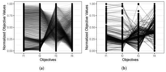
Figure 3.
Parallel coordinate plots of the LSID problem for (a) the reference Pareto and (b) the non-dominated solutions obtained by the MOWOA/D.
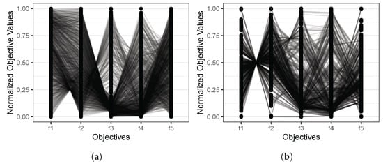
Figure 4.
Parallel coordinate plots of the UWAD problem for (a) the reference Pareto and (b) the non-dominated solutions obtained by the MOWOA/D.
Figure 3 shows the parallel plots for the liquid-rocket single-element injector design problem [82]. The plot in Figure 3a, which corresponds to the Pareto reference set, depicts that there is no conflict for the first pair of objectives, but there is in the other two pairs. As shown in Figure 3b, the same relations between pairs of objectives are present in the non-dominated solutions found by the MOWOA/D.
For the ultra-wideband antenna design [85], we can observe that the parallel plots of the Pareto reference set (Figure 4a) evidence that there is conflict in each pair of objectives, something that the non-dominated solutions found by the MOWOA/D (Figure 4b) also proved.
After this analysis, it can be concluded that solving these real-world multi-objective problems is difficult, not only because of the number of objective functions but also because of the conflict that exists between the objectives.
7. Conclusions
This research introduced and examined a Multi-objective Whale Optimization Algorithm based on decomposition (MOWOA/D). The decomposition technique, commonly employed in conventional multi-criteria methods, converts a multi-objective problem into multiple single-objective subproblems. The MOWOA/D approximates Pareto optimal solutions by concurrently solving these scalarized subproblems. Each subproblem is assigned to a sub-group of whales, selected from the entire population, which work together to approximate the Pareto front of the multi-objective problem. The effectiveness of the MOWOA/D was demonstrated through experiments on well-known benchmark problems from the UF test suite and two real-world engineering applications. A thorough evaluation was conducted to assess the performance of the MOWOA/D with varying neighborhood sizes and updated position selection probabilities. Comparative analysis revealed that the MOWOA/D consistently outperformed state-of-the-art MOEAs and the standard MOWOA, which uses Pareto optimality for environmental selection. These results highlight the advantages of incorporating multi-objective decomposition for solving complex optimization problems. Particularly, the proposed algorithm demonstrated superior effectiveness in solving real-world applications with four or five objective functions.
Some limitations and disadvantages of the MOWOA/D include the fact that the algorithm was applied only for unconstrained optimization problems, continuous optimization problems, and problems without many objectives. Future research will focus on extending the MOWOA/D to address constrained multi-objective problems. Additionally, integrating single-objective mathematical programming techniques into the MOWOA/D will be explored, and this hybrid approach is expected to lead to significant performance improvements. Applying the MOWOA/D to real-world problems, which often require diverse heuristics due to their unknown characteristics, is another promising direction. Given that the MOWOA/D is a relatively recent development, its potential in practical applications remains largely unexplored. Further studies will also aim to develop a version of the MOWOA that incorporates performance indicators to enhance optimization outcomes.
Author Contributions
Conceptualization, S.Z.-M. and D.O.; Formal analysis, J.R.-F., A.C.-O., S.Z.-M., D.O. and A.G.-N.; Funding acquisition, M.P.-C.; Investigation, J.R.-F., A.C.-O., S.Z.-M., D.O., A.V.-G. and A.G.-N.; Methodology, S.Z.-M.; Software, J.R.-F. and A.C.-O.; Validation, J.R.-F., A.C.-O., S.Z.-M. and A.G.-N.; Visualization, A.G.-N.; Writing—original draft, J.R.-F., A.C.-O., S.Z.-M., D.O., A.V.-G., A.G.-N. and M.P.-C.; Writing—review and editing, J.R.-F., A.C.-O., S.Z.-M., D.O., A.V.-G., A.G.-N. and M.P.-C. All authors have read and agreed to the published version of the manuscript.
Funding
This research received no external funding.
Data Availability Statement
The original contributions presented in the study are included in the article; further inquiries can be directed to the corresponding author.
Conflicts of Interest
The authors have no competing interests to declare relevant to this article’s content. All authors certify that they have no affiliations with or involvement in any organization or entity with any financial interest or non-financial interest in the subject or materials discussed in this manuscript.
References
- Kennedy, J.; Eberhart, R. Particle swarm optimization. In Proceedings of the ICNN’95-International Conference on Neural Networks, Perth, Australia, 27 November–1 December 1995; Volume 4, pp. 1942–1948. [Google Scholar]
- Dorigo, M.; Birattari, M.; Stutzle, T. Ant colony optimization. IEEE Comput. Intell. Mag. 2006, 1, 28–39. [Google Scholar] [CrossRef]
- Karaboga, D.; Basturk, B. Artificial bee colony (ABC) optimization algorithm for solving constrained optimization problems. In Proceedings of the International Fuzzy Systems Association World Congress, Cancun, Mexico, 18–21 June 2007; Springer: Berlin/Heidelberg, Germany, 2007; pp. 789–798. [Google Scholar]
- Mirjalili, S.; Mirjalili, S.M.; Lewis, A. Grey wolf optimizer. Adv. Eng. Softw. 2014, 69, 46–61. [Google Scholar] [CrossRef]
- Mirjalili, S.; Lewis, A. The whale optimization algorithm. Adv. Eng. Softw. 2016, 95, 51–67. [Google Scholar] [CrossRef]
- Dao, T.K.; Pan, T.S.; Pan, J.S. A multi-objective optimal mobile robot path planning based on whale optimization algorithm. In Proceedings of the 2016 IEEE 13th International Conference on Signal Processing (ICSP), Chengdu, China, 6–10 November 2016; pp. 337–342. [Google Scholar]
- Aziz, M.A.E.; Ewees, A.A.; Hassanien, A.E. Multi-objective whale optimization algorithm for content-based image retrieval. Multimed. Tools Appl. 2018, 77, 26135–26172. [Google Scholar] [CrossRef]
- Kumawat, I.R.; Nanda, S.J.; Maddila, R.K. Multi-objective whale optimization. In Proceedings of the Tencon 2017–2017 IEEE Region 10 Conference, Penang, Malaysia, 5–8 November 2017; pp. 2747–2752. [Google Scholar]
- Islam, Q.N.U.; Ahmed, A.; Abdullah, S.M. Optimized controller design for islanded microgrid using non-dominated sorting whale optimization algorithm (NSWOA). Ain Shams Eng. J. 2021, 12, 3677–3689. [Google Scholar] [CrossRef]
- Coello, C.A.C. Evolutionary Algorithms for Solving Multi-Objective Problems; Springer: Berlin/Heidelberg, Germany, 2007. [Google Scholar]
- Miettinen, K. Nonlinear Multiobjective Optimization; Kluwer Academic Publishers: Boston, MA, USA, 1999. [Google Scholar]
- Srinivas, N.; Deb, K. Multiobjective Optimization Using Nondominated Sorting in Genetic Algorithms. Evol. Comput. 1994, 2, 221–248. [Google Scholar] [CrossRef]
- Goldberg, D.E. Genetic Algorithms in Search, Optimization and Machine Learning; Addison-Wesley Publishing Company: Reading, MA, USA, 1989. [Google Scholar]
- Zitzler, E.; Laumanns, M.; Thiele, L. SPEA2: Improving the Strength Pareto Evolutionary Algorithm. In Proceedings of the EUROGEN 2001. Evolutionary Methods for Design, Optimization and Control with Applications to Industrial Problems; Giannakoglou, K., Tsahalis, D., Periaux, J., Papailou, P., Fogarty, T., Eds.; ETH Zurich, Computer Engineering and Networks Laboratory: Athens, Greece, 2002; pp. 95–100. [Google Scholar]
- Deb, K.; Goldberg, D.E. An Investigation of Niche and Species Formation in Genetic Function Optimization. In Proceedings of the Third International Conference on Genetic Algorithms; Schaffer, J.D., Ed.; George Mason University: San Mateo, CA, USA, 1989; pp. 42–50. [Google Scholar]
- Deb, K.; Pratap, A.; Agarwal, S.; Meyarivan, T. A fast and elitist multiobjective genetic algorithm: NSGA-II. IEEE Trans. Evol. Comput. 2002, 6, 182–197. [Google Scholar] [CrossRef]
- Farhang-Mehr, A.; Azarm, S. Diversity Assessment of Pareto Optimal Solution Sets: An Entropy Approach. In Proceedings of the Congress on Evolutionary Computation (CEC’2002), Piscataway, NJ, USA, 12–17 May 2002; Volume 1, pp. 723–728. [Google Scholar]
- Hallam, N.; Blanchfield, P.; Kendall, G. Handling Diversity in Evolutionary Multiobjective Optimisation. In Proceedings of the 2005 IEEE Congress on Evolutionary Computation (CEC’2005), Edinburgh, UK, 2–5 September 2005; Volume 3, pp. 2233–2240. [Google Scholar]
- Gee, S.B.; Tan, K.C.; Shim, V.A.; Pal, N.R. Online Diversity Assessment in Evolutionary Multiobjective Optimization: A Geometrical Perspective. IEEE Trans. Evol. Comput. 2015, 19, 542–559. [Google Scholar] [CrossRef]
- López Jaimes, A.; Coello Coello, C.A. Many-objective Problems: Challenges and Methods. In Springer Handbook of Computational Intelligence; Kacprzyk, J., Pedrycz, W., Eds.; Springer: Berlin/Heidelberg, Germany, 2015; Chapter 51; pp. 1033–1046. [Google Scholar]
- Brockhoff, D.; Zitzler, E. Are All Objectives Necessary? On Dimensionality Reduction in Evolutionary Multiobjective Optimization. In Parallel Problem Solving from Nature—PPSN IX, 9th International Conference; Runarsson, T.P., Beyer, H.G., Burke, E., Merelo-Guervós, J.J., Whitley, L.D., Yao, X., Eds.; Lecture Notes in Computer Science Volume 4193: Reykjavik, Iceland; Springer: Berlin/Heidelberg, Germany, 2006; pp. 533–542. [Google Scholar]
- Zitzler, E.; Künzli, S. Indicator-based Selection in Multiobjective Search. In Proceedings of the Parallel Problem Solving from Nature—PPSN VIII, Birmingham, UK, 18–22 September 2004; Yao, X., Burke, E.K., Lozano, J.A., Smith, J., Merelo-Guervós, J.J., Bullinaria, J.A., Rowe, J.E., Tiňo, P., Kabán, A., Schwefel, H.-P., Eds.; pp. 832–842. [Google Scholar]
- Coello Coello, C.; Reyes Sierra, M. A study of the parallelization of a coevolutionary multi-objective evolutionary algorithm. In Proceedings of the MICAI 2004: Advances in Artificial Intelligence: Third Mexican International Conference on Artificial Intelligence, Mexico City, Mexico, 26–30 April 2004; Proceedings 3. Springer: Berlin/Heidelberg, Germany, 2004; pp. 688–697. [Google Scholar]
- Hansen, M.P.; Jaszkiewicz, A. Evaluating the Quality of Approximations to the Non-Dominated Set; Technical Report IMM-REP-1998-7; Technical University of Denmark: Kongens Lyngby, Denmark, 1998. [Google Scholar]
- Zitzler, E.; Thiele, L. Multiobjective optimization using evolutionary algorithms—A comparative case study. In Proceedings of the International Conference on Parallel Problem Solving from Nature, Amsterdam, The Netherlands, 27–30 September 1998; Springer: Berlin/Heidelberg, Germany, 1998; pp. 292–301. [Google Scholar]
- Zapotecas-Martínez, S.; Sosa Hernández, V.A.; Aguirre, H.; Tanaka, K.; Coello Coello, C.A. Using a Family of Curves to Approximate the Pareto Front of a Multi-Objective Optimization Problem. In Parallel Problem Solving from Nature—PPSN XIII, 13th International Conference, Ljubljana, Slovenia, 13–17 September 2014; Bartz-Beielstein, T., Branke, J., Filipic, B., Smith, J., Eds.; Lecture Notes in Computer Science; Springer: Berlin/Heidelberg, Germany, 2014; Volume 8672, pp. 682–691. [Google Scholar]
- Hernández Gómez, R.; Coello Coello, C.A. Improved metaheuristic based on the R2 indicator for many-objective optimization. In Proceedings of the 2015 Annual Conference on Genetic and Evolutionary Computation, Madrid, Spain, 11–15 July 2015; pp. 679–686. [Google Scholar]
- Zapotecas-Martínez, S.; López-Jaimes, A.; García-Nájera, A. LIBEA: A Lebesgue Indicator-Based Evolutionary Algorithm for multi-objective optimization. Swarm Evol. Comput. 2019, 44, 404–419. [Google Scholar] [CrossRef]
- Zapotecas-Martínez, S.; García-Nájera, A.; Menchaca-Méndez, A. Improved Lebesgue indicator-based evolutionary algorithm: Reducing hypervolume computations. Mathematics 2022, 10, 19. [Google Scholar] [CrossRef]
- Zhang, Q.; Li, H. MOEA/D: A multiobjective evolutionary algorithm based on decomposition. IEEE Trans. Evol. Comput. 2007, 11, 712–731. [Google Scholar] [CrossRef]
- Li, H.; Zhang, Q. Multiobjective optimization problems with complicated Pareto sets, MOEA/D and NSGA-II. IEEE Trans. Evol. Comput. 2008, 13, 284–302. [Google Scholar] [CrossRef]
- Zhang, Q.; Zhou, A.; Jin, Y. RM-MEDA: A Regularity Model-Based Multiobjective Estimation of Distribution Algorithm. IEEE Trans. Evol. Comput. 2008, 12, 41–63. [Google Scholar] [CrossRef]
- Li, K.; Deb, K.; Zhang, Q.; Kwong, S. An evolutionary many-objective optimization algorithm based on dominance and decomposition. IEEE Trans. Evol. Comput. 2015, 19, 694–716. [Google Scholar] [CrossRef]
- Peng, W.; Zhang, Q. A decomposition-based multi-objective particle swarm optimization algorithm for continuous optimization problems. In Proceedings of the 2008 IEEE International Conference on Granular Computing, Hangzhou, China, 26–28 August 2008; pp. 534–537. [Google Scholar]
- Zapotecas-Martínez, S.; Coello Coello, C.A. A Multi-objective Particle Swarm Optimizer Based on Decomposition. In Proceedings of the 13th Annual Conference on Genetic and Evolutionary Computation, Dublin, Ireland, 12–16 July 2011; Association for Computing Machinery: New York, NY, USA, 2011. GECCO ’11. pp. 69–76. [Google Scholar]
- Zapotecas-Martínez, S.; Garcia-Najera, A.; Lopez-Jaimes, A. Multi-objective grey wolf optimizer based on decomposition. Expert Syst. Appl. 2019, 120, 357–371. [Google Scholar] [CrossRef]
- Zhou, A.; Qu, B.Y.; Li, H.; Zhao, S.Z.; Suganthan, P.N.; Zhang, Q. Multiobjective evolutionary algorithms: A survey of the state of the art. Swarm Evol. Comput. 2011, 1, 32–49. [Google Scholar] [CrossRef]
- Nedjah, N.; de Macedo Mourelle, L. Evolutionary multi-objective optimisation: A survey. Int. J. Bio-Inspired Comput. 2015, 7, 1–25. [Google Scholar] [CrossRef]
- Trivedi, A.; Srinivasan, D.; Sanyal, K.; Ghosh, A. A Survey of Multiobjective Evolutionary Algorithms Based on Decomposition. IEEE Trans. Evol. Comput. 2017, 21, 440–462. [Google Scholar] [CrossRef]
- Bowman, V.J., Jr. On the relationship of the Tchebycheff norm and the efficient frontier of multiple-criteria objectives. In Proceedings of the Multiple Criteria Decision Making: Proceedings of a Conference, Jouy-en-Josas, France, 21–23 May 1975; Springer: Berlin/Heidelberg, Germany, 1976; pp. 76–86. [Google Scholar]
- Kasturi, K.; Nayak, M.R. Optimal planning of charging station for EVs with PV-BES unit in distribution system using WOA. In Proceedings of the 2017 2nd International Conference on Man and Machine Interfacing (MAMI), Bhubaneswar, India, 21–23 December 2017; pp. 1–6. [Google Scholar]
- El Aziz, M.A.; Ewees, A.A.; Hassanien, A.E.; Mudhsh, M.; Xiong, S. Multi-objective whale optimization algorithm for multilevel thresholding segmentation. In Advances in Soft Computing and Machine Learning in Image Processing; Springer: Cham, Switzerland, 2018; pp. 23–39. [Google Scholar]
- Narendrababu Reddy, G.; Kumar, S.P. Multi objective task scheduling algorithm for cloud computing using whale optimization technique. In Proceedings of the Smart and Innovative Trends in Next Generation Computing Technologies: Third International Conference, NGCT 2017, Dehradun, India, 30–31 October 2017; Revised Selected Papers, Part I 3. Springer: Berlin/Heidelberg, Germany, 2018; pp. 286–297. [Google Scholar]
- Siddiqi, F.A.; Mofizur Rahman, C. Evolutionary multi-objective whale optimization algorithm. In Proceedings of the Intelligent Systems Design and Applications: 18th International Conference on Intelligent Systems Design and Applications (ISDA 2018), Vellore, India, 6–8 December 2018; Springer: Berlin/Heidelberg, Germany, 2020; Volume 2, pp. 431–446. [Google Scholar]
- Shayeghi, H.; Alilou, M.; Tousi, B.; Dadkhah Doltabad, R. Sizing and Placement of DG and UPQC for Improving the Profitability of Distribution System Using Multi-objective WOA. In Proceedings of the Intelligent Systems Design and Applications: 18th International Conference on Intelligent Systems Design and Applications (ISDA 2018), Vellore, India, 6–8 December 2018; Springer: Berlin/Heidelberg, Germany, 2020; Volume 2, pp. 810–820. [Google Scholar]
- Wang, W.L.; Li, W.K.; Wang, Z.; Li, L. Opposition-based multi-objective whale optimization algorithm with global grid ranking. Neurocomputing 2019, 341, 41–59. [Google Scholar] [CrossRef]
- Ahmed, M.M.; Houssein, E.H.; Hassanien, A.E.; Taha, A.; Hassanien, E. Maximizing lifetime of large-scale wireless sensor networks using multi-objective whale optimization algorithm. Telecommun. Syst. 2019, 72, 243–259. [Google Scholar] [CrossRef]
- Saleh, A.A.; Mohamed, A.A.A.; Hemeida, A.; Ibrahim, A.A. Multi-objective whale optimization algorithm for optimal allocation of distributed generation and capacitor bank. In Proceedings of the 2019 International Conference on Innovative Trends in Computer Engineering (ITCE), Aswan, Egypt, 2–4 February 2019; pp. 459–465. [Google Scholar]
- Yin, X.; Cheng, L.; Wang, X.; Lu, J.; Qin, H. Optimization for hydro-photovoltaic-wind power generation system based on a modified version of multi-objective whale optimization algorithm. Energy Procedia 2019, 158, 6208–6216. [Google Scholar] [CrossRef]
- Ishibuchi, H.; Murata, T. A multi-objective genetic local search algorithm and its application to flowshop scheduling. IEEE Trans. Syst. Man, Cybern. Part C Appl. Rev. 1998, 28, 392–403. [Google Scholar] [CrossRef]
- Zhang, Q.; Liu, W.; Li, H. The performance of a new version of MOEA/D on CEC09 unconstrained MOP test instances. In Proceedings of the 2009 IEEE Congress on Evolutionary Computation, Trondheim, Norway, 18–21 May 2009; pp. 203–208. [Google Scholar]
- Liu, Y.; Niu, B. A multi-objective particle swarm optimization based on decomposition. In Proceedings of the Emerging Intelligent Computing Technology and Applications: 9th International Conference, ICIC 2013, Nanning, China, 28–31 July 2013; Proceedings 9. Springer: Berlin/Heidelberg, Germany, 2013; pp. 200–205. [Google Scholar]
- Al Moubayed, N.; Petrovski, A.; McCall, J. D2MOPSO: MOPSO based on decomposition and dominance with archiving using crowding distance in objective and solution spaces. Evol. Comput. 2014, 22, 47–77. [Google Scholar] [CrossRef]
- Dai, C.; Wang, Y.; Ye, M. A new multi-objective particle swarm optimization algorithm based on decomposition. Inf. Sci. 2015, 325, 541–557. [Google Scholar] [CrossRef]
- Akbari, R.; Hedayatzadeh, R.; Ziarati, K.; Hassanizadeh, B. A multi-objective artificial bee colony algorithm. Swarm Evol. Comput. 2012, 2, 39–52. [Google Scholar] [CrossRef]
- Karaboga, D.; Basturk, B. A powerful and efficient algorithm for numerical function optimization: Artificial bee colony (ABC) algorithm. J. Glob. Optim. 2007, 39, 459–471. [Google Scholar] [CrossRef]
- Akay, B.; Karaboga, D. A modified artificial bee colony algorithm for real-parameter optimization. Inf. Sci. 2012, 192, 120–142. [Google Scholar] [CrossRef]
- Medina, M.A.; Das, S.; Coello, C.A.C.; Ramírez, J.M. Decomposition-based modern metaheuristic algorithms for multi-objective optimal power flow–A comparative study. Eng. Appl. Artif. Intell. 2014, 32, 10–20. [Google Scholar] [CrossRef]
- Rao, R.V.; Savsani, V.J.; Vakharia, D.P. Teaching–learning-based optimization: A novel method for constrained mechanical design optimization problems. Comput.-Aided Des. 2011, 43, 303–315. [Google Scholar] [CrossRef]
- Ganesh, N.; Shankar, R.; Kalita, K.; Jangir, P.; Oliva, D.; Pérez-Cisneros, M. A novel decomposition-based multi-objective symbiotic organism search optimization algorithm. Mathematics 2023, 11, 1898. [Google Scholar] [CrossRef]
- Chen, L.; Gan, W.; Li, H.; Cheng, K.; Pan, D.; Chen, L.; Zhang, Z. Solving multi-objective optimization problem using cuckoo search algorithm based on decomposition. Appl. Intell. 2021, 51, 143–160. [Google Scholar] [CrossRef]
- Ning, J.; Zhao, Q.; Sun, P.; Feng, Y. A multi-objective decomposition-based ant colony optimisation algorithm with negative pheromone. J. Exp. Theor. Artif. Intell. 2021, 33, 827–845. [Google Scholar] [CrossRef]
- Zhao, H.; Zhang, C.; Zhang, B. A decomposition-based many-objective ant colony optimization algorithm with adaptive reference points. Inf. Sci. 2020, 540, 435–448. [Google Scholar] [CrossRef]
- Li, L.; Lin, Q.; Liu, S.; Gong, D.; Coello, C.A.C.; Ming, Z. A novel multi-objective immune algorithm with a decomposition-based clonal selection. Appl. Soft Comput. 2019, 81, 105490. [Google Scholar] [CrossRef]
- Das, I.; Dennis, J.E. Normal-boundary intersection: A new method for generating Pareto optimal points in multicriteria optimization problems. SIAM J. Optim. 1998, 8, 631–657. [Google Scholar] [CrossRef]
- Tawhid, M.A.; Savsani, V. Multi-objective sine-cosine algorithm (MO-SCA) for multi-objective engineering design problems. Neural Comput. Appl. 2019, 31, 915–929. [Google Scholar] [CrossRef]
- Zhang, Q.; Zhou, A.; Zhao, S.; Suganthan, P.N.; Liu, W.; Tiwari, S. Multiobjective Optimization Test Instances for the CEC 2009 Special Session and Competition; Technical report; University of Essex: Colchester, UK, 2008. [Google Scholar]
- Scheffé, H. Experiments With Mixtures. J. R. Stat. Soc. 1958, 20, 344–360. [Google Scholar] [CrossRef]
- Sierra, M.R.; Coello, C.A.C. Improving PSO-Based Multi-objective Optimization Using Crowding, Mutation and epsilon-Dominance. In Proceedings of the Evolutionary Multi-Criterion Optimization, Third International Conference, EMO 2005, Guanajuato, Mexico, 9–11 March 2005; Proceedings. Coello, C.A.C., Aguirre, A.H., Zitzler, E., Eds.; Lecture Notes in Computer Science. Springer: Berlin/Heidelberg, Germany, 2005; Volume 3410, pp. 505–519. [Google Scholar]
- Moubayed, N.A.; Petrovski, A.; McCall, J.A.W. A Novel Smart Multi-Objective Particle Swarm Optimisation Using Decomposition. In Proceedings of the PPSN (2), Kraków, Poland, 11–15 September 2010; pp. 1–10. [Google Scholar]
- Okabe, T.; Jin, Y.; Sendhoff, B. A Critical Survey of Performance Indices for Multi-Objective Optimization. In Proceedings of the 2003 Congress on Evolutionary Computation (CEC’2003), Canberra, Australia, 8–12 December 2003; Volume 2, pp. 878–885.
- Zitzler, E.; Thiele, L.; Laumanns, M.; Fonseca, C.M.; Da Fonseca, V.G. Performance assessment of multiobjective optimizers: An analysis and review. IEEE Trans. Evol. Comput. 2003, 7, 117–132. [Google Scholar] [CrossRef]
- Knowles, J.D.; Thiele, L.; Zitzler, E. A tutorial on the performance assessment of stochastic multiobjective optimizers. Tik Rep. 2006, 214. [Google Scholar]
- Van Veldhuizen, D.A.; Lamont, G.B. Multiobjective Evolutionary Algorithm Research: A History and Analysis; Technical Report; Department of Electrical and Computer Engineering, Graduate School of Engineering, Air Force Institute of Technology: Wright-Patterson AFB, OH, USA, 1998. [Google Scholar]
- Van Veldhuizen, D.A. Multiobjective Evolutionary Algorithms: Classifications, Analyses, and New Innovations; Air Force Institute of Technology: Dayton, OH, USA, 1999. [Google Scholar]
- Ishibuchi, H.; Masuda, H.; Tanigaki, Y.; Nojima, Y. Modified distance calculation in generational distance and inverted generational distance. In Proceedings of the Evolutionary Multi-Criterion Optimization: 8th International Conference, EMO 2015, Guimarães, Portugal, 29 March–1 April 2015; Proceedings, Part II 8. Springer: Berlin/Heidelberg, Germany, 2015; pp. 110–125. [Google Scholar]
- Montero, E.; Zapotecas-Martínez, S. An Analysis of Parameters of Decomposition-Based MOEAs on Many-Objective Optimization. In Proceedings of the 2018 IEEE Congress on Evolutionary Computation (CEC), Rio de Janeiro, Brazil, 8–13 July 2018; pp. 1–8. [Google Scholar]
- Wilcoxon, F. Individual comparisons by ranking methods. In Breakthroughs in Statistics: Methodology and Distribution; Springer: Berlin/Heidelberg, Germany, 1992; pp. 196–202. [Google Scholar]
- Bonferroni, C. Teoria statistica delle classi e calcolo delle probabilita. Pubbl. R Ist. Super. Sci. Econ. Commericiali Firenze 1936, 8, 3–62. [Google Scholar]
- Gill, G.; Nurick, W. Liquid Rocket Engine Injectors; Technical Report. 1976. Available online: https://ntrs.nasa.gov/citations/19760023196 (accessed on 1 February 2025).
- Calhoon, D.; Ito, J.; Kors, D. Design Handbook for Gaseous Fuel Engine Injectors and Combustion Chambers. NASA Tech Brief, LEW-12154, Report Number: LEW-12154, Lewis Research Center. December 1973. Available online: https://ntrs.nasa.gov/citations/19730000412 (accessed on 1 February 2025).
- Vaidyanathan, R.; Tucker, K.; Papila, N.; Shyy, W. Computational-Fluid-Dynamics-Based Design Optimization for Single-Element Rocket Injector. J. Propuls. Power 2004, 20, 705–717. [Google Scholar] [CrossRef]
- Goel, T.; Vaidyanathan, R.; Haftka, R.T.; Shyy, W.; Queipo, N.V.; Tucker, K. Response surface approximation of Pareto optimal front in multi-objective optimization. Comput. Methods Appl. Mech. Eng. 2007, 196, 879–893. [Google Scholar] [CrossRef]
- Chen, Y.S. Performance enhancement of multiband antennas through a two-stage optimization technique. Int. J. RF Microw. Comput.-Aided Eng. 2017, 27, e21064. [Google Scholar] [CrossRef]
- Chen, Y.S. Multiobjective optimization of complex antenna structures using response surface models. Int. J. RF Microw. Comput.-Aided Eng. 2016, 26, 62–71. [Google Scholar] [CrossRef]
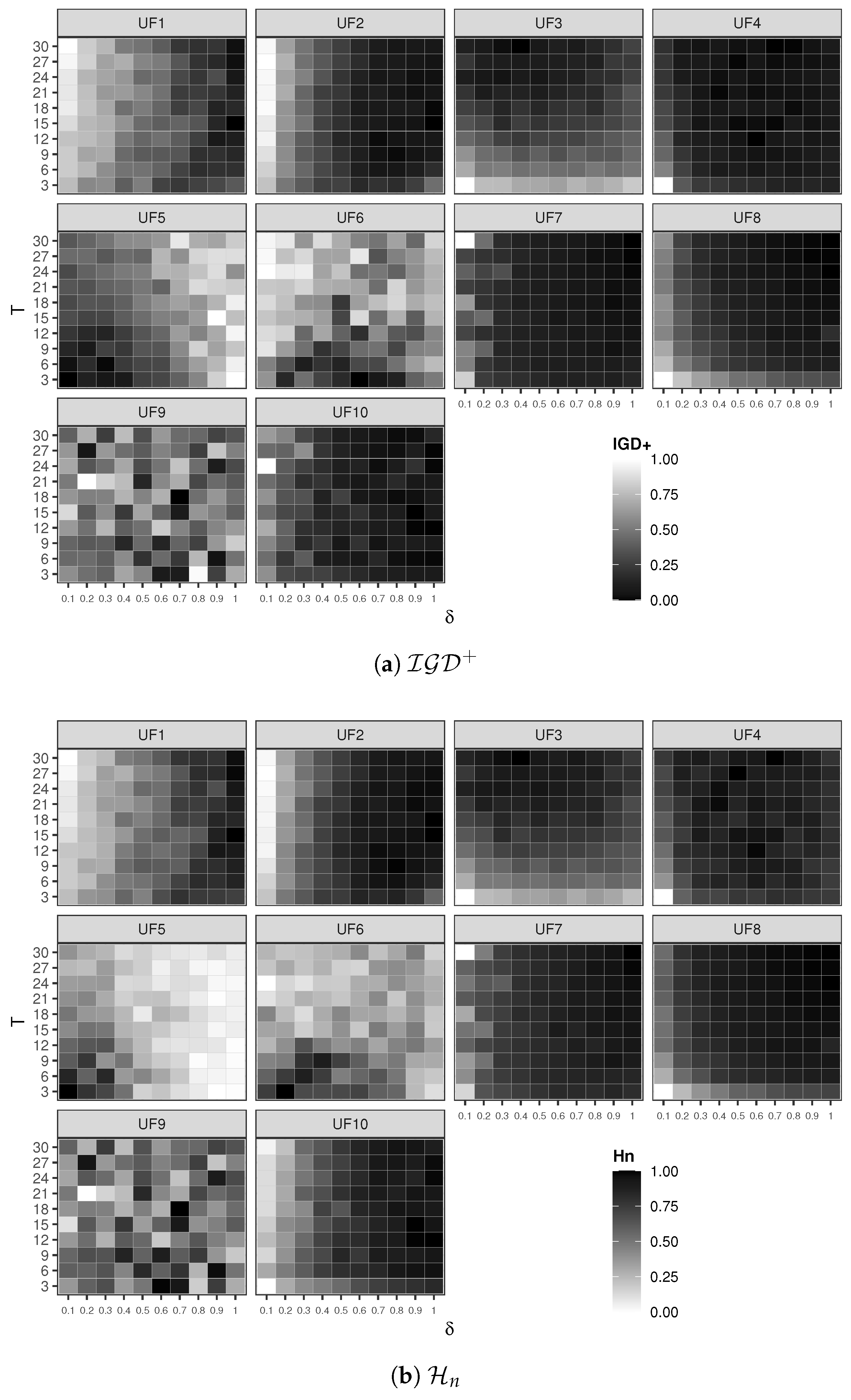
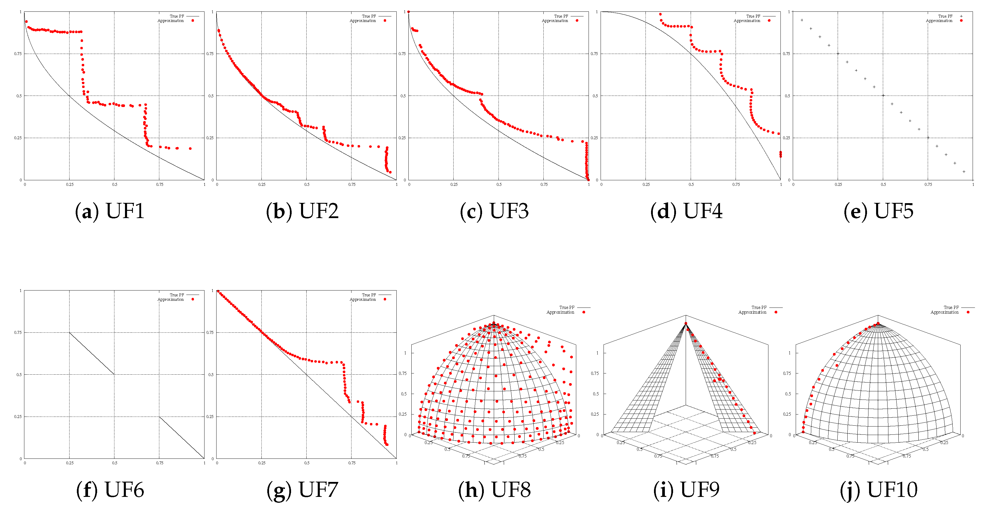
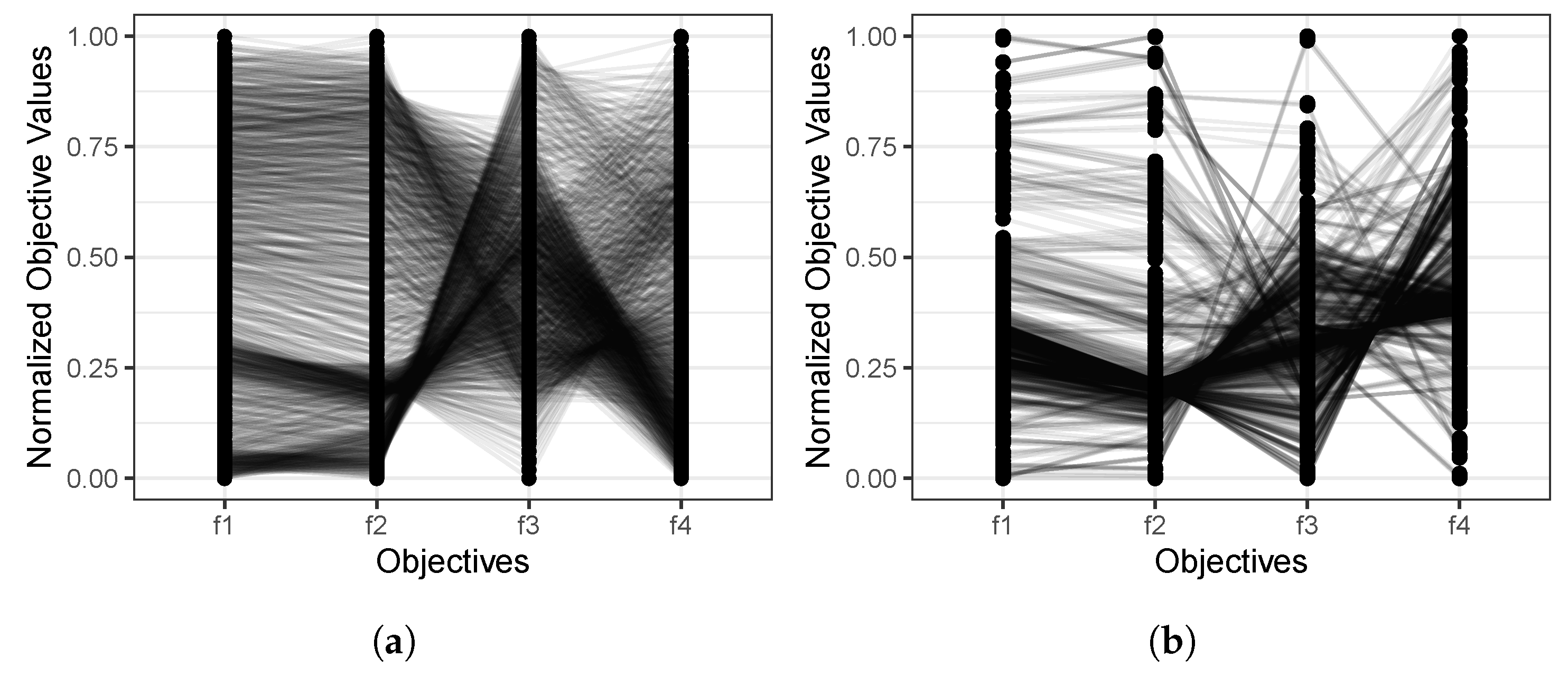
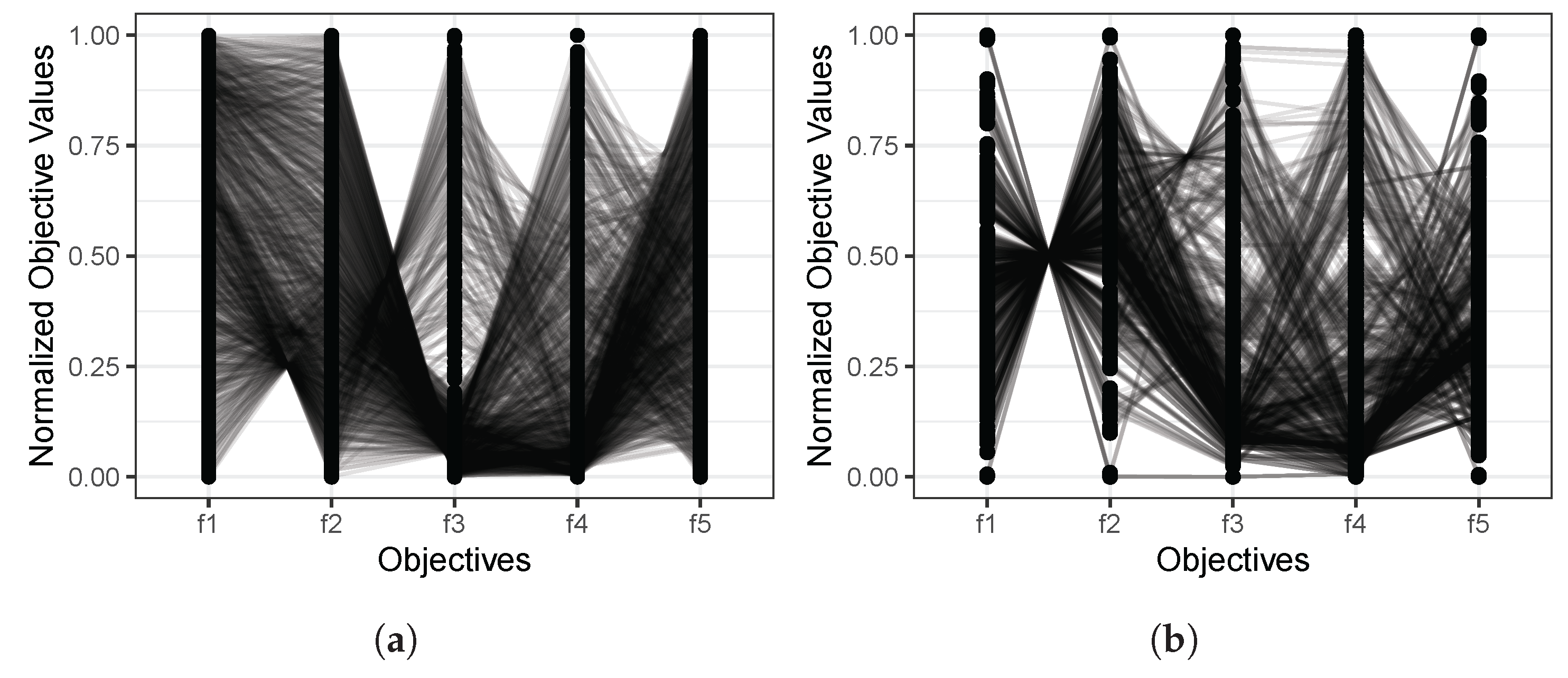
Disclaimer/Publisher’s Note: The statements, opinions and data contained in all publications are solely those of the individual author(s) and contributor(s) and not of MDPI and/or the editor(s). MDPI and/or the editor(s) disclaim responsibility for any injury to people or property resulting from any ideas, methods, instructions or products referred to in the content. |
© 2025 by the authors. Licensee MDPI, Basel, Switzerland. This article is an open access article distributed under the terms and conditions of the Creative Commons Attribution (CC BY) license (https://creativecommons.org/licenses/by/4.0/).