Deep Learning Artificial Neural Network for Pricing Multi-Asset European Options

Abstract

This paper studies a p-layers deep learning artificial neural network (DLANN) for European multi-asset options. Firstly, a p-layers DLANN is constructed with undetermined weights and bias. Secondly, according to the terminal values of the partial differential equation (PDE) and the points that satisfy the PDE of multi-asset options, some discrete data are fed into the p-layers DLANN. Thirdly, using the least square error as the objective function, the weights and bias of the DLANN are trained well. In order to optimize the objective function, the partial derivatives for the weights and bias of DLANN are carefully derived. Moreover, to improve the computational efficiency, a time-segment DLANN is proposed. Numerical examples are presented to confirm the accuracy, efficiency, and stability of the proposed p-layers DLANN. Computational examples show that the DLANN’s relative error is less than $0.5\%$ for different numbers of assets $d=1,2,3,4$. In the future, the p-layers DLANN can be extended into American options, Asian options, Lookback options, and so on.

1. Introduction

In the last 30 years, different methods and techniques for multi-asset option pricing have been developed. For options pricing on one to three assets, the radial basis function (RBF) method uses the so-called radial basis function to approximate European and American options [1,2,3,4,5,6,7,8,9,10]. For the low-dimensional case, the semi-analytical solutions and analytical solutions of a European option and an American option can be obtained [11,12]. The finite difference (FD) method for solving an option’s partial differential equation (PDE) was derived under the Black–Scholes model and Heston model [13,14,15,16,17]. A Monte Carlo simulation for SABA options of calorimeter systems and multi-asset options was proposed [18,19,20]. Laplace transform or Mellin transform methods for some classical options have been presented [15,21,22,23,24]. The willow tree (WT) method under Lévy processes was established [25,26].

In general, for RBF, FD, and WT methods, only some cases with lower dimensions ($d\le 2$) can be solved easily. For analytical or semi-analytical methods, these can only be applied to some simple or classical options. Although Monte Carlo simulation is suitable for any high-dimensional problem, it is computationally inefficient, resulting in a significant consumption of CPU time and storage space. Therefore, Monte Carlo methods are limited to simple models and are computationally heavy.

In the past decade, several scholars have applied artificial neural networks (ANNs) to solve option values. Anderson and Ulrich used deep neural networks to price American options [27]. Caverhill et al. proposed an ANN method for option pricing and hedging [28]. Based on the residual ANN, Gan and Liu discussed option pricing [29]. Kapllani and Teng provided a deep learning artificial neural network to solve nonlinear backward stochastic differential equations (BSDE) [30]. For estimating option prices, Lee and Son used artificial neural networks to predict arbitrage-free American options [31]. Mary and Salchenberger proposed an ANN model [32] to estimate option prices. Nikolas and Lorenz discussed a deep learning method to interpolate between BSDEs and PINNs [33]. Robert Balkin et al. considered a machine learning algorithm to solve stochastic delay differential equations [34]. Teng et al. discussed combining artificial neural networks with classical volatility prediction models for option pricing [35,36]. Umeorah, Mashele, and Agbaeze provided a barrier option pricing method with an ANN [37]. Wang proposed an artificial neural network prediction model for stock index options [38]. All of these BSDE-based approaches, however, do not come directly from the option’s PDE.

Unlike general data fitting problems, there are many difficulties in using artificial neural networks in option pricing. We know that these options satisfy the Black–Scholes PDE. In order to apply artificial neural network to option pricing, proper discretization of the PDE must be carried out. Using an artificial neural network to approximate the PDE of an option is the main difficulty and innovation of this paper.

In this paper, a p-layers deep learning (DLANN) is considered for multi-dimensional option pricing. After a p-layers DLANN is established, the PDE of a multi-asset option is expressed in the ANN. By minimizing the objective functions in the DLANN, all parameters (including the weights and bias) are trained well. The deep learning p-ANN is relatively easy to implement, shows the capability for multi-asset option pricing, and is much faster than other schemes (such as a Monte Carlo simulation). It is noted that this paper is an improved version of Zhou and Wu [39].

This paper is arranged as follows. In Section 2, we introduce the PDE of a multi-asset model. In Section 3, a $p\sim$ layers deep learning ANN ($p\sim$ DLANN) computational frame is proposed. The derivatives of the p-DLANN’s weights and bias are listed. Then, the updated formulas of the weights and bias in the $p\sim$ DLANN are given. Section 4 lists some examples to confirm the efficiency and accuracy of the proposed algorithms. In Section 5, some conclusions and future work are proposed. Finally, Appendix A provides some appendices, including derivative formulas of the weights and bias and some computational results.

2. Model of Multi-Asset Options

Let $\mathit{S}={(S_1\left(t\right),S_2\left(t\right),\dots ,S_d\left(t\right))}^{\prime }$, with ${(·)}^{\prime }$ denoting the transposition of $(·)$, be d-asset prices at time t, and let $ln{S}_I\left(t\right),I=1,2,\dots ,d$, be modeled by Brownian motion together with a drift term under a no-arbitrage assumption, i.e., $S_I\left(t\right)$ are controlled by stochastic differential equations (SDEs),

$$\begin{array}{c}\hfill \mathrm{d}ln{S}_I\left(t\right)={\displaystyle \frac{\mathrm{d}{S}_I\left(t\right)}{S_I\left(t\right)}}=(r-q_I)\mathrm{d}t+{\sigma }_I\mathrm{d}{W}_t^{\left(I\right)},I=1,2,\dots ,d.\end{array}$$

(1)

In SDEs (1), r represents the risk-free interest, $q_I$ represents the dividend yield, and ${\sigma }_I$ represents the volatility of asset I. $W_t^{\left(I\right)},I=1,2,\dots ,d$, are d standard Brownian motions, and it is assumed that

$$\begin{array}{c}\hfill \left\{\begin{array}{c}\mathbb{E}\left(\mathrm{d}{W}_t^{\left(I\right)}\right)=0,Var\left(\mathrm{d}{W}_t^{\left(I\right)}\right)=\mathrm{d}t,I=1,2,\dots ,d,\hfill \\ Cov\left(\mathrm{d}{W}_t^{\left(I\right)},\mathrm{d}{W}_t^{\left(J\right)}\right)={\rho }_{IJ}\mathrm{d}t,I,J=1,2,\dots ,d,\hfill \end{array}\right.,\end{array}$$

(2)

where ${\rho }_{IJ}$ are the coefficients of association between $\mathrm{d}{W}_t^{\left(I\right)}$ and $\mathrm{d}{W}_t^{\left(J\right)}$. Then, the PDE of the d-asset option value $V(t,\mathit{x})$ emerges as

$$\begin{array}{c}\hfill {\displaystyle \frac{\partial V(t,\mathit{S})}{\partial t}}+{\displaystyle \frac{1}{2}}\sum _{I=1}^d\sum _{J=1}^d{\rho }_{IJ}{\sigma }_I{\sigma }_J{S}_I{S}_J{\displaystyle \frac{{\partial }^{2}V(t,\mathit{S})}{\partial S_I\partial S_J}}+\sum _{I=1}^d(r-q_I)S_I{\displaystyle \frac{\partial V(t,\mathit{S})}{\partial S_I}}-rV(t,\mathit{S}),t\in (0,T),\mathit{S}\in {\mathrm{\Omega }}_S,\end{array}$$

(3)

where $\mathit{S}={(S_1\left(t\right),S_2\left(t\right),\dots ,S_d\left(t\right))}^{\prime }\in {\mathrm{\Omega }}_S={(0,+\infty )}^d$.

Let the remainder time to maturity $\tau =T-t$, and $x_I\left(t\right)=ln{S}_I\left(t\right)$ for $I=1,2,\dots ,d$; then, the d-asset option value $v(\tau ,\mathit{x})=V(T-t,\mathit{x})$ is re-written as

$$\begin{array}{c}\hfill {\displaystyle \frac{\partial v}{\partial \tau }}(\tau ,\mathit{x})-\mathcal{A}v(\tau ,\mathit{x})=0,\tau \in (0,T),\mathit{x}\in \mathrm{\Omega },\end{array}$$

(4)

where $\mathit{x}={(x_1\left(t\right),x_2\left(t\right),\dots ,x_d\left(t\right))}^{\prime }\in \mathrm{\Omega }={(-\infty ,+\infty )}^d$, and the linear differential operator $\mathcal{A}$ is defined as

$$\begin{array}{c}\hfill \mathcal{A}:={\displaystyle \frac{1}{2}}\sum _{I=1}^d\sum _{J=1}^d{a}_{IJ}{\displaystyle \frac{{\partial }^2}{\partial x_I\partial x_J}}+\sum _{I=1}^d{b}_I{\displaystyle \frac{\partial }{\partial x_I}}-r,\end{array}$$

(5)

with coefficients $a_{IJ}:={\rho }_{IJ}{\sigma }_I{\sigma }_J$ and $b_I:=r-q_I-{\displaystyle \frac{1}{2}}{a}_{II}$.

For a European option, $v(\tau ,\mathit{x})$ has the initial values (also called terminal conditions or payoff functions, for time $\tau =0$)

$$\begin{array}{c}\hfill v(0,\mathit{x})=\mathrm{\Pi }\left(\mathit{x}\right).\end{array}$$

(6)

System (4)–(6) can be written as

$$\begin{array}{c}\hfill \left\{\begin{array}{c}{\displaystyle \frac{\partial v}{\partial \tau }}(\tau ,\mathit{x})-\mathcal{A}v(\tau ,\mathit{x})=0,\tau \in (0,T],\mathit{x}\in \mathrm{\Omega },\hfill \\ v(0,\mathit{x})=\mathrm{\Pi }\left(\mathit{x}\right),\mathit{x}\in \mathrm{\Omega }.\hfill \end{array}\right.\end{array}$$

(7)

For put options and geometric mean payoff functions $\mathrm{\Pi }\left(\mathit{x}\right)$, the initial values of v are taken as

$$\begin{array}{c}\hfill v(0,\mathit{x})=\mathrm{\Pi }\left(\mathit{x}\right)=max\left(0,K-e^{{\displaystyle \sum _{I=1}^d{\alpha }_I{x}_I}}\right),0\le {\alpha }_I\le 1,\sum _{I=1}^d{\alpha }_I=1,\forall \mathit{x}\in \mathrm{\Omega },\end{array}$$

(8)

with strike price K. In the general case, System (7) has no analytical solutions, and a certain numerical method is needed to determine the option value $v(\tau ,\mathit{x})$ in domain $(0,T]\times \mathrm{\Omega }$, for example, the Monte Carlo simulation, RBF numerical solution, finite difference method, and artificial neural network method.

With the geometric mean payoff function $\mathrm{\Pi }\left(\mathit{x}\right)$ defined by (8), the put option governed by System (7) has an analytical solution (see Expression (42)). However, for a put option with an arithmetic mean payoff function

$$\begin{array}{c}\hfill \mathrm{\Pi }\left(\mathit{x}\right)=max\left(0,K-\sum _{I=1}^d{\alpha }_I{e}^{x_I}\right),0\le {\alpha }_I\le 1,\sum _I^d{\alpha }_I=1,\forall \mathit{x}\in \mathrm{\Omega },\end{array}$$

(9)

the option $v(\tau ,\mathit{x})$ has no analytical solution. So, the numerical scheme is a feasible method to price a multi-asset option governed by (7) and (9). In this paper, we propose a p-layers DLANN to price the multi-asset option values.

3. Computational Frame of $p\sim$ DLANN

3.1. Structure of $p\sim$ DLANN

A deep learning artificial neural network (DLANN) is defined as shown in Figure 1. In Figure 1, the p-layers ANN includes an input layer, $p-2$ hidden layers, and an output layer. For an example, the neural units in five layers are $n_1=d+1,n_2=4,n_3=5,n_4=4$, and $n_5=1$. We will see in Section 4 that this structure is powerful for some European option pricing.

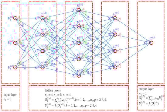
Figure 1. Graphical depiction of the artificial neural network with a input layer, three hidden layers, and a output layer.

The evolution of the p-layers DLANN is represented as matrix expressions,

$$\begin{array}{c}\hfill \left\{\begin{array}{c}{\mathit{O}}^{(\ell )}={\mathit{\omega }}^{(\ell )}{\mathit{U}}^{(\ell -1)}+{\mathit{\theta }}^{(\ell )},\ell =2,3,\dots ,p,\hfill \\ {\mathit{U}}^{(\ell )}=f_{\ell }\left({\mathit{O}}^{(\ell )}\right),\ell =2,3,\dots ,p,\hfill \end{array}\right.\end{array}$$

(10)

where ${\mathit{O}}^{(\ell )}$ is the input data in the ${\ell }^{\mathrm{th}}$ layer, ${\mathit{U}}^{(\ell )}$ is the output in the layer ℓ, and $f_{\ell }$ is the transform function (or activation function). The algebraic expression is given by

$$\begin{array}{c}\hfill \left\{\begin{array}{c}{\displaystyle O_j^{(\ell )}=\sum _{i=1}^{n_{\ell -1}}{\omega }_{ji}^{(\ell )}{U}_i^{(\ell -1)}+{\theta }_j^{(\ell )},j=1,2,\dots ,n_{\ell };\ell =2,3,\dots ,p,}\hfill \\ U_j^{(\ell )}=f_{\ell }\left(O_j^{(\ell )}\right),j=1,2,\dots ,n_{\ell };\ell =2,3\dots ,p,\hfill \end{array}\right.\end{array}$$

(11)

where $U^{\left(1\right)}$ is a $(d+1)$ input data column vector ${(x_1,x_2,\dots ,x_d,\tau )}^{\prime }$, and $f_{\ell }(·)(\ell =2,3,\dots ,p)$ are the activation functions, i.e.,

$$\begin{array}{c}\hfill f_{\ell }\left(x\right)={\displaystyle \frac{1}{1+e^{-x}}}(\ell =2,\dots ,p-1,\mathrm{sigmoid}\mathrm{function}),f_p\left(x\right)=x\left(\mathrm{linear}\mathrm{function}\right).\end{array}$$

(12)

The derivatives $f_{\ell }^{\prime }\left(U\right)$ and $f_{\ell }^{″}\left(U\right)$ are

$$\begin{array}{c}\hfill f_{\ell }^{\prime }\left(O\right)=\left\{\begin{array}{cc}1,\hfill & \ell =p,\hfill \\ U(1-U),\hfill & \ell <p,\hfill \end{array}\right.\mathrm{and}{f}_{\ell }^{″}\left(O\right)=\left\{\begin{array}{cc}0,\hfill & \ell =p,\hfill \\ U(1-U)(1-2U),\hfill & \ell <p,\hfill \end{array}\right.\end{array}$$

(13)

which can be found in Appendix A.2. The activation function $f_{\ell }\left(x\right)$ can be used in other functions, but this paper only uses functions in the above form.

The weights and bias in the ANN are defined as

$$\begin{array}{c}\hfill {\mathit{\omega }}^{(\ell )}=\left[\begin{array}{cccc}{\omega }_{11}^{(\ell )}& {\omega }_{12}^{(\ell )}& \dots & {\omega }_{1n_{\ell -1}}^{(\ell )}\\ {\omega }_{21}^{(\ell )}& {\omega }_{22}^{(\ell )}& \dots & {\omega }_{2n_{\ell -1}}^{(\ell )}\\ ⋮& ⋮& ⋮& ⋮\\ {\omega }_{n_{\ell }1}^{(\ell )}& {\omega }_{n_{\ell }2}^{(\ell )}& \dots & {\omega }_{n_{\ell }{n}_{\ell -1}}^{(\ell )}\end{array}\right],{\mathit{\theta }}^{(\ell )}=\left[\begin{array}{c}{\theta }_1^{(\ell )}\\ {\theta }_2^{(\ell )}\\ ⋮\\ {\theta }_{n_{\ell }}^{(\ell )}\end{array}\right],\end{array}$$

(14)

for $\ell =2,3,\dots ,p$. We call (10) or (11) a p-layers deep learning artificial neural network (denoted as p-DLANN). Using the p-DLANN network has the following challenges:

(1)

It is relatively hard to compute the partial derivatives, $\mathrm{\Delta }{\omega }_{IJ}^{(\ell )}$ and $\mathrm{\Delta }{\theta }_I^{(\ell )}$, for $\ell =2,\dots ,p$, $I=1,2,\cdots ,n_{\ell }$, and $J=1,2,\cdots ,n_{\ell -1}$. We must update the parameters ${\omega }_{IJ}^{(\ell )}={\omega }_{IJ}^{(\ell )}-\eta \mathrm{\Delta }{\omega }_{IJ}^{(\ell )}$ and ${\theta }_I^{(\ell )}={\theta }_I^{(\ell )}-\eta \mathrm{\Delta }{\theta }_I^{(\ell )}$ with the appropriate leaning rate $\eta$.

(2)

For a deep learning neural network p-DLANN ($p>3$), it is somewhat complicated to compute the partial derivatives of ${\omega }_{IJ}^{(\ell )}$ and ${\theta }_I^{(\ell )}$ for $\ell =2,3,\cdots ,p$ and $I=1,2,\cdots ,n_{\ell },J=1,2,\cdots ,n_{\ell -1}$.

(3)

In option pricing, to use the deep learning networks p-DLANN to solve the PDE, we must first obtain the discrete PDE.

The output of the network is denoted by

$$\begin{array}{c}\hfill {\mathit{U}}^{(\ell )}\left(\mathit{X}\right)=\left\{U_1^{(\ell )}\left(\mathit{X}\right),U_2^{(\ell )}\left(\mathit{X}\right),\dots ,U_{n_{\ell }}^{(\ell )}\left(\mathit{X}\right)\right\},\ell =p,p-1,\dots ,2,\end{array}$$

(15)

with input data ${\mathit{U}}^{\left(1\right)}=\mathit{X}={\left[x_1,x_2,\dots ,x_d,\tau \right]}^{\prime }$. We denote by $v(\tau ,\mathit{x}):=U_1^{\left(p\right)}\left(\mathit{X}\right)=net\left(\mathit{\omega },\mathit{\theta },\mathit{X}\right)$ the network output with input data $\mathit{X}$ under parameters $\left\{\mathit{\omega },\mathit{\theta }\right\}$. In addition, we denote by ${\mathit{U}}^{(\ell ,k)}={\mathit{U}}^{(\ell )}\left({\mathit{X}}^{\left(k\right)}\right),\ell =1,2,\dots ,p$ with N space and time input data

$$\begin{array}{c}\hfill {\mathit{X}}^{\left(k\right)}={\left[x_1^{\left(k\right)},x_2^{\left(k\right)},\dots ,x_d^{\left(k\right)},{\tau }^{\left(k\right)}\right]}^{\prime },k=1,2,\dots ,N.\end{array}$$

(16)

The purpose of our p-DLANN structure is to determine the optimal weights $\mathit{\omega }$ and bias $\mathit{\theta }$. For this purpose, we use an iteration algorithm, i.e., we modify the values of the parameters $\mathit{\omega }$ and $\mathit{\theta }$ until some objective function $MSE$ is less than the pre-specified error $\epsilon$.

For convenience, we list some of the symbols used in this paper in Table 1.

Table 1. Some symbols for $p\sim$ DLANN.

Name	Meaning
$N^{\prime }$	The number of data, which are the initial conditions
N	The number of input data for the training of DLANN
$N-N^{\prime }$	The input number of data for the discrete PDE
$net\left({\{{\mathit{\omega }}^{(\ell )},{\mathit{\theta }}^{(\ell )}\}}_{\ell =2}^p\right)$	$p\sim$ DLANN with weights ${\left\{{\mathit{\omega }}^{(\ell )}\right\}}_{\ell =2}^p$ and bias ${\left\{{\mathit{\theta }}^{(\ell )}\right\}}_{\ell =2}^p$
$v(\tau ,\mathit{x})=U_1^p\left(\mathit{X}\right)=net\left({\{{\mathit{\omega }}^{(\ell )},{\mathit{\theta }}^{(\ell )}\}}_{\ell =2}^p,\mathit{X}\right)$	$p\sim$ DLANN output with input data $\mathit{X}={(x_1,x_2,\dots ,x_d,\tau )}^{\prime }$
$\eta$	Learning rate of DLANN
${\mathit{O}}_k^{(\ell )}$	Input data at the ℓ-layer ($\ell =2,3,\dots ,p;k=1,2,\dots ,n_p$)
${\mathit{U}}_k^{(\ell )}$	Output data at the ℓ-layer ($\ell =1,2,\dots ,p;k=1,2,\dots ,n_p$)
$MS{E}^{\left(payoff\right)}$	Error for the payoff functions or initial values
$MS{E}^{\left(PDE\right)}$	Error for the discrete PDE
$\mathrm{\Delta }{\mathit{\theta }}^{(payoff,k)}$, $\mathrm{\Delta }{\mathit{\theta }}^{(PDE,k)}$	Partial derivatives of $\mathit{\theta }$ for kth input data
$\mathrm{\Delta }{\mathit{\omega }}^{(payoff,k)}$, $\mathrm{\Delta }{\mathit{\omega }}^{(PDE,k)}$	Partial derivatives of $\mathit{\omega }$ for kth input data
$\mathrm{D}$	Partial derivatives for $\mathit{x}$ with $\mathrm{D}={\mathrm{D}}_{\tau },\mathrm{D}={\mathrm{D}}_I$, and $\mathrm{D}={\mathrm{D}}_{IJ}$

In the following paragraphs, we give the definition of the objective function for the DLANN, the mean square error (MSE),

$$\begin{array}{c}\hfill MSE=MS{E}^{\left(payoff\right)}+MS{E}^{\left(PDE\right)},\end{array}$$

(17)

with $MS{E}^{\left(payoff\right)}$ being the error at points ${\mathit{X}}^{\left(k\right)}=\left(x_1^{\left(k\right)},\dots ,x_d^{\left(k\right)},{\tau }_1\right)$, with $k=1,2,\dots ,N^{\prime }$ and ${\tau }_1=0$, and $MS{E}^{\left(PDE\right)}$ being the error of the PDE (7), with ${\mathit{X}}^{\left(k\right)}=\left(x_1^{\left(k\right)},\dots ,x_d^{\left(k\right)},{\tau }^{\left(k\right)}\right)$ and ${\tau }^{\left(k\right)}$ being one of values

$$\begin{array}{c}\hfill {\tau }^{\left(k\right)}=\mathrm{\Delta }\tau ,\dots ,{\tau }_j,\dots ,{\tau }_M=T.\end{array}$$

(18)

3.2. Update of Weights and Bias

Firstly, we consider the $MS{E}^{\left(payoff\right)}$ at ${\tau }_1=0$.

For the initial conditions, we have $U_1^{\left(p\right)}\left({\mathit{X}}^{\left(k\right)}\right)=v(0,\mathit{x})=\mathrm{\Pi }\left({\mathit{x}}^{\left(k\right)}\right)=y^{\left(k\right)},k=1,2,\dots ,N^{\prime }$. Then, the $MS{E}^{\left(payoff\right)}$ of p-DLANN at ${\tau }_0=0$ is defined by

$$\begin{array}{c}\hfill MS{E}^{\left(payoff\right)}={\displaystyle \frac{1}{2N^{\prime }}}\sum _{k=1}^{N^{\prime }}{\left(U_1^{(p,k)}-y^{\left(k\right)}\right)}^2:={\displaystyle \frac{1}{2N^{\prime }}}\sum _{k=1}^{N^{\prime }}S{E}_k^{\left(payoff\right)}.\end{array}$$

(19)

The partial derivatives of $MS{E}_k^{\left(payoff\right)}$ with respect to the weights ${\omega }_{IJ}^{(\ell )}$ are

$$\begin{array}{c}\hfill {\displaystyle \frac{\partial S{E}_k^{\left(payoff\right)}}{\partial {\omega }_{IJ}^{(\ell )}}}={\displaystyle \frac{\partial S{E}_k^{\left(payoff\right)}}{\partial U_1^{(p,k)}}}{\displaystyle \frac{\partial U_1^{(p,k)}}{\partial {\omega }_{IJ}^{(\ell )}}}=2\left(U_1^{(p,k)}-y^{\left(k\right)}\right){\displaystyle \frac{\partial U_1^{(p,k)}}{\partial {\omega }_{IJ}^{(\ell )}}},\end{array}$$

(20)

for $I=1,2,\cdots ,n_{\ell }$, $J=1,2,\cdots ,n_{\ell -1}$, and $\ell =2,3,\cdots ,p$.

In detail, we have

$$\begin{array}{c}\hfill \left\{\begin{array}{c}{\displaystyle \frac{\partial U_1^{(p,k)}}{\partial {\omega }_{1J}^{\left(p\right)}}=U_J^{(p-1,k)},}\hfill \\ {\displaystyle \frac{\partial U_1^{(p,k)}}{\partial {\omega }_{IJ}^{(p-1)}}={\omega }_{1I}^{\left(p\right)}g\left(U_I^{(p-1,k)}\right)U_J^{(p-2,k)},}\hfill \\ {\displaystyle \frac{\partial U_1^{(p,k)}}{\partial {\omega }_{IJ}^{(p-2)}}=g\left(U_I^{(p-2,k)}\right)U_J^{(p-3,k)}\sum _{j=1}^{n_{p-1}}{\omega }_{1j}^{\left(p\right)}{\omega }_{jI}^{(p-1)}g\left(U_j^{(p-1,k)}\right),}\hfill \\ {\displaystyle \frac{\partial U_1^{(p,k)}}{\partial {\omega }_{IJ}^{(p-3)}}=g\left(U_I^{(p-3,k)}\right)U_J^{(p-4,k)}\sum _{j_1=1}^{n_{p-1}}{\omega }_{1j_1}^{\left(p\right)}g\left(U_{j_1}^{(p-1,k)}\right)\sum _{j_2=1}^{n_{p-2}}{\omega }_{j_1{j}_2}^{(p-1)}g\left(U_{j_2}^{(p-2,k)}\right){\omega }_{j_{2}I}^{(p-2)},}\hfill \\ \hfill \cdots \cdots \hfill \\ {\displaystyle \frac{\partial U_1^{(p,k)}}{\partial {\omega }_{IJ}^{(p-\ell )}}=g\left(U_I^{(p-\ell ,k)}\right)U_J^{(p-(\ell +1),k)}\sum _{j_1=1}^{n_{p-1}}{\omega }_{1j_1}^{\left(p\right)}g\left(U_{j_1}^{(p-1,k)}\right)\sum _{j_2=1}^{n_{p-2}}{\omega }_{j_1{j}_2}^{(p-1)}g\left(U_{j_2}^{(p-2,k)}\right)\cdots \cdots }\hfill \\ {\displaystyle \sum _{j_{\ell -1}=1}^{n_{p-(\ell -1)}}{\omega }_{j_{\ell -2}{j}_{\ell -1}}^{(p-(\ell -2\left)\right)}g\left(U_{j_{\ell -1}}^{(p-(\ell -1),k)}\right){\omega }_{j_{\ell -1}I}^{(p-(\ell -1\left)\right)},}\hfill \end{array}\right.\end{array}$$

(21)

for $I=1,2,\dots ,n_{p-\ell }$, $J=1,2,\dots ,n_{p-\ell -1}$, and $\ell =0,1,\cdots ,p-2$ with function

$$\begin{array}{c}\hfill g\left(U\right)=f_{\ell }^{\prime }\left(O\right)=U(1-U),\ell =2,3,\cdots ,p-1.\end{array}$$

(22)

The deduction of (21) can be found in Appendix A.1.1.

The partial derivatives of $S{E}_k^{\left(payoff\right)}$ with respect to ${\theta }_I^{(\ell )}$ are

$$\begin{array}{c}\hfill {\displaystyle \frac{\partial S{E}_k^{\left(payoff\right)}}{\partial {\theta }_I^{(\ell )}}}={\displaystyle \frac{\partial S{E}_k^{\left(payoff\right)}}{\partial U_1^{(p,k)}}}{\displaystyle \frac{\partial U_1^{(p,k)}}{\partial {\theta }_I^{(\ell )}}}=2\left(U_1^{(p,k)}-y^{\left(k\right)}\right){\displaystyle \frac{\partial U_1^{(p,k)}}{\partial {\theta }_I^{(\ell )}}},\end{array}$$

(23)

for $I=1,2,\dots ,n_{\ell }$ and $\ell =2,3,\dots ,p$. In detail, we have

$$\begin{array}{c}\hfill \left\{\begin{array}{c}{\displaystyle \frac{\partial U_1^{(p,k)}}{\partial {\theta }_I^{\left(p\right)}}}=1,I=1,2,\dots ,n_p,\hfill \\ {\displaystyle \frac{\partial U_1^{(p,k)}}{\partial {\theta }_I^{(p-1)}}}={\omega }_{1I}^{\left(p\right)}g\left(U_I^{(p-1,k)}\right),I=1,2,\dots ,n_{p-1},\hfill \\ {\displaystyle \frac{\partial U_1^{(p,k)}}{\partial {\theta }_I^{(p-2)}}=g\left(U_I^{(p-2,k)}\right)\sum _{j=1}^{n_{p-1}}{\omega }_{1j}^{\left(p\right)}g\left(U_j^{(p-1,k)}\right){\omega }_{jI}^{(p-1)},I=1,2,\dots ,n_{p-2},}\hfill \\ {\displaystyle \frac{\partial U_1^{(p,k)}}{\partial {\theta }_I^{(p-3)}}=g\left(U_I^{(p-3,k)}\right)\sum _{j_1=1}^{n_{p-1}}{\omega }_{1j_1}^{\left(p\right)}g\left(U_{j_1}^{(p-1,k)}\right)\sum _{j_2=1}^{n_{p-2}}{\omega }_{j_1{j}_2}^{(p-1)}g\left(U_{j_2}^{(p-2,k)}\right){\omega }_{j_{2}I}^{(p-2)},I=1,2,\dots ,n_{p-3}}\hfill \\ \hfill \cdots \cdots \hfill \\ {\displaystyle \frac{\partial U_1^{(p,k)}}{\partial {\theta }_I^{(p-\ell )}}=g\left(U_I^{(p-\ell ,k)}\right)\sum _{j_1=1}^{n_{p-1}}{\omega }_{1j_1}^{\left(p\right)}g\left(U_{j_1}^{(p-1,k)}\right)\sum _{j_2=1}^{n_{p-2}}{\omega }_{j_1{j}_2}^{(p-1)}g\left(U_{j_2}^{(p-2,k)}\right)\cdots \cdots \sum _{j_{\ell -1}=1}^{n_{p-(\ell -1)}}{\omega }_{j_{\ell -2}{j}_{\ell -1}}^{(p-(\ell -2\left)\right)}}\hfill \\ ·g\left(U_{j_{\ell -1}}^{(p-(\ell -1),k)}\right){\omega }_{j_{\ell -1}I}^{(p-(\ell -1\left)\right)},I=1,2,\dots ,n_{p-\ell },\ell =0,1,\dots ,p-2.\hfill \end{array}\right.\end{array}$$

(24)

The deduction of (24) can be seen in Appendix A.1.2. Observing (21) and (24), we have a relationship between $\partial U_1^{(p,k)}/\partial {\omega }_{IJ}^{(\ell )}$ and $\partial U_1^{(p,k)}/\partial {\theta }_I^{(\ell )}$,

$$\begin{array}{c}\hfill {\displaystyle \frac{\partial U_1^{(p,k)}}{\partial {\omega }_{IJ}^{(\ell )}}}=U_J^{(\ell -1,k)}{\displaystyle \frac{\partial U_1^{(p,k)}}{\partial {\theta }_I^{(\ell )}}},\end{array}$$

(25)

for $\ell =2,3,\cdots ,p$, $I=1,2,\cdots ,n_{\ell }$, and $J=1,2,\cdots ,n_{\ell -1}$. This relationship can simplify our computation and save some CPU time.

Let the increments of ${\omega }_{\ell ,I,J}^{\left(payoff\right)}$ and ${\theta }_{\ell ,I}^{\left(payoff\right)}$ be as follows:

$$\left\{\begin{array}{c}{\displaystyle \mathrm{\Delta }{\theta }_{\ell ,I}^{\left(payoff\right)}=\frac{1}{2N^{\prime }}\sum _{k=1}^{N^{\prime }}\frac{\partial S{E}_k^{\left(payoff\right)}}{\partial {\theta }_I^{(\ell )}},}\hfill \\ \hfill {\displaystyle \mathrm{\Delta }{\omega }_{\ell ,I,J}^{\left(payoff\right)}=\frac{1}{2N^{\prime }}\sum _{k=1}^{N^{\prime }}\frac{\partial S{E}_k^{\left(payoff\right)}}{\partial {\omega }_{IJ}^{(\ell )}}=\frac{1}{2N^{\prime }}\sum _{k=1}^{N^{\prime }}{U}_J^{(\ell -1)}\frac{\partial S{E}_k^{\left(payoff\right)}}{\partial {\theta }_I^{(\ell )}},}\end{array}\right.$$

(26)

with the definition of partial derivatives (21) and (24).

Secondly, we discuss the $MS{E}^{\left(PDE\right)}$ at discrete points ${\mathit{X}}^{\left(k\right)}$ for $k=N^{\prime }+1,2,\dots ,N$. The discrete error $MS{E}^{\left(PDE\right)}$ of PDE at points ${\mathit{X}}^{\left(k\right)}$ are defined as

$$\begin{array}{ccc}\hfill MS{E}^{\left(PDE\right)}& :=& {\displaystyle \frac{1}{2(N-N^{\prime })}}\sum _{k=N^{\prime }+1}^{N}PD{E}_{p,k}^2,\hfill \end{array}$$

(27)

where

$$\begin{array}{ccc}\hfill PD{E}_{p,k}& :=& {\left[{\displaystyle \frac{\partial U(\tau ,\mathit{x})}{\partial \tau }}-\mathcal{A}U(\tau ,\mathit{x})\right]}_{\mathit{X}={\mathit{X}}^{\left(k\right)}}\hfill \\ & \approx & {\mathrm{D}}_{\tau }{U}_1^{(p,k)}-\sum _{I=1}^d\sum _{J=1}^d{a}_{IJ}{\mathrm{D}}_{IJ}{U}_1^{(p,k)}-\sum _{I=1}^d{b}_I{\mathrm{D}}_I{U}_1^{(p,k)}+r{U}_1^{(p,k)},\hfill \end{array}$$

(28)

for $k=N^{\prime }+1,\dots ,N$. Here, differential operators ${\mathrm{D}}_{\tau }:=\partial /\partial \tau ,{\mathrm{D}}_I:=\partial /\partial x_I$, and ${\mathrm{D}}_{IJ}:={\partial }^2/\partial x_I\partial x_J$.

The partial derivatives $\partial /\partial x_I{U}_{\kappa }^{(\ell ,k)}$ are recursively computed as

$$\begin{array}{ccc}\hfill {\displaystyle \frac{\partial }{\partial x_I}}{U}_{\kappa }^{(\ell ,k)}& :=& \begin{array}{|c|}\hline D_I{U}_{\kappa }^{(\ell ,k)}\\ \hline\end{array}={\displaystyle \frac{\partial U_{\kappa }^{(\ell ,k)}}{\partial O_{\kappa }^{(\ell ,k)}}}\sum _{q=1}^{n_{\ell -1}}{\displaystyle \frac{\partial O_{\kappa }^{(\ell ,k)}}{\partial U_q^{(\ell -1,k)}}}\begin{array}{|c|}\hline {\displaystyle \frac{\partial U_q^{(\ell -1,k)}}{\partial x_I}}\\ \hline\end{array}\hfill \\ & =& f_{\ell }^{\prime }\left(O_{\kappa }\right)\sum _{q=1}^{n_{\ell -1}}{\omega }_{\kappa q}^{(\ell )}\begin{array}{|c|}\hline D_I{U}_q^{(\ell -1,k)}\\ \hline\end{array},\hfill \end{array}$$

(29)

for

$$\begin{array}{c}\hfill I=1,2,\dots ,d+1;\ell =p,p-1,\dots ,2;\kappa =1,2,\dots ,n_{\ell };k=N^{\prime }+1,N^{\prime }+2,\dots ,N.\end{array}$$

(30)

By careful analysis, we have recursive derivation formulas ${\partial }^2{U}_{\kappa }^{(\ell ,k)}/\partial x_I\partial x_J$ as follows:

$$\begin{array}{ccc}\hfill {\displaystyle \frac{{\partial }^2{U}_{\kappa }^{(\ell ,k)}}{\partial x_I\partial x_J}}& =& \begin{array}{|c|}\hline {\mathrm{D}}_{IJ}{U}_{\kappa }^{(\ell ,k)}\\ \hline\end{array}=f_{\ell }^{\prime }\left(O_{\kappa }^{(\ell ,k)}\right)\sum _{q=1}^{n_{\ell -1}}{\omega }_{kq}^{(\ell )}\begin{array}{|c|}\hline {\mathrm{D}}_{IJ}{U}_q^{(\ell -1,k)}\\ \hline\end{array}\hfill \\ & +& f_{\ell }^{″}\left(O_{\kappa }^{(\ell ,k)}\right)\left(\sum _{q=1}^{n_{\ell -1}}{\omega }_{\kappa q}^{(\ell )}\begin{array}{|c|}\hline {\mathrm{D}}_I{U}_q^{(\ell -1,k)}\\ \hline\end{array}\right)\left(\sum _{q=1}^{n_{\ell -1}}{\omega }_{\kappa q}^{(\ell )}\begin{array}{|c|}\hline {\mathrm{D}}_J{U}_q^{(\ell -1,k)}\\ \hline\end{array}\right),\hfill \end{array}$$

(31)

for $\ell =p,p-1,\dots ,2$;$\kappa =1,2,\dots ,n_{\ell }$; $I,J=1,2,\dots ,d$; and $k=N^{\prime }+1,2,\cdots ,N$, with  $f_{\ell }^{\prime }\left(O\right)$ and $f_{\ell }^{″}\left(O\right)$ being defined in (13). In Equation (31), the derivatives ${\mathrm{D}}_I{U}_q^{(\ell -1,q)}$ and ${\mathrm{D}}_J{U}_q^{(\ell -1,q)}$ are defined as in (29).

The terminate values in (29) and (31) are set as

$$\begin{array}{c}\hfill {\mathrm{D}}_I{U}_{\kappa }^{(1,k)}\left\{\begin{array}{cc}1,\hfill & I=\kappa ,\hfill \\ 0,\hfill & I\ne \kappa ,\hfill \end{array}\right.\mathrm{for}I=1,2,\dots d+1\mathrm{and}{\mathrm{D}}_{IJ}{U}_{\kappa }^{(1,k)}=0\mathrm{for}I,J=1,2,\dots ,d.\end{array}$$

(32)

We define the partial derivatives

$$\begin{array}{ccc}\hfill {\displaystyle \frac{\partial MS{E}^{\left(PDE\right)}}{\partial {\omega }_{IJ}^{(\ell )}}}& =& {\displaystyle \frac{1}{2(N-N^{\prime })}}\sum _{k=N^{\prime }+1}^N{\displaystyle \frac{\partial PD{E}_{p,k}^2}{\partial {\omega }_{IJ}^{(\ell )}}},\hfill \end{array}$$

(33)

for $\ell =2,\dots ,p$, $I=1,2,\dots ,n_{\ell }$, and $J=1,2,\dots ,n_{\ell -1}$. We define the partial derivatives

$$\begin{array}{ccc}\hfill {\displaystyle \frac{\partial MS{E}^{\left(PDE\right)}}{\partial {\theta }_J^{(\ell )}}}& =& {\displaystyle \frac{1}{2(N-N^{\prime })}}\sum _{k=N^{\prime }+1}^N{\displaystyle \frac{\partial PD{E}_{p,k}^2}{\partial {\theta }_J^{(\ell )}}},\hfill \end{array}$$

(34)

for $\ell =p,p-1,\dots ,2$ and $J=1,2,\dots ,n_{\ell }$.

The partial derivatives ${\displaystyle \frac{1}{2}}\partial PD{E}_{p,k}^2/\partial {\omega }_{IJ}^{(\ell )}$ in (33) are found as

$$\begin{array}{ccc}\hfill & & {\displaystyle \frac{1}{2}}{\displaystyle \frac{\partial PD{E}_{p,k}^2}{\partial {\omega }_{IJ}^{(\ell )}}}=PD{E}_{p,k}{\displaystyle \frac{\partial PD{E}_{p,k}}{\partial {\omega }_{IJ}^{(\ell )}}}\hfill \\ & =& PD{E}_{p,k}\left\{{\displaystyle \frac{\partial \left({\mathrm{D}}_{\tau }{U}_1^{(p,k)}\right)}{\partial {\omega }_{IJ}^{(\ell )}}}-{\displaystyle \frac{1}{2}}\sum _{i=1}^d\sum _{j=1}^d{a}_{ij}{\displaystyle \frac{\partial \left({\mathrm{D}}_{ij}{U}_1^{(p,k)}\right)}{\partial {\omega }_{IJ}^{(\ell )}}}-\sum _{i=1}^d{b}_i{\displaystyle \frac{\partial \left({\mathrm{D}}_i{U}_1^{(p,k)}\right)}{\partial {\omega }_{IJ}^{(\ell )}}}+r{\displaystyle \frac{\partial U_1^{(p,k)}}{\partial {\omega }_{IJ}^{(\ell )}}}\right\},\hfill \end{array}$$

(35)

for $\ell =p,p-1,\dots ,2$, $I=1,2,\dots ,n_{\ell }$, and $J=1,2,\dots ,n_{\ell -1}$. The partial derivatives ${\displaystyle \frac{1}{2}}\partial PD{E}_{p,k}^2/\partial {\theta }_J^{(\ell )}$ in (34) are found as

$$\begin{array}{ccc}\hfill & & {\displaystyle \frac{1}{2}}{\displaystyle \frac{\partial PD{E}_{p,k}^2}{\partial {\theta }_J^{(\ell )}}}=PD{E}_{p,k}{\displaystyle \frac{\partial PD{E}_{p,k}}{\partial {\theta }_J^{(\ell )}}}\hfill \\ & =& PD{E}_{p,k}\left\{{\displaystyle \frac{\partial {\mathrm{D}}_{\tau }{U}_1^{(p,k)}}{\partial {\theta }_J^{(\ell )}}}-{\displaystyle \frac{1}{2}}\sum _{i=1}^d\sum _{j=1}^d{a}_{ij}{\displaystyle \frac{\partial \left({\mathrm{D}}_{ij}{U}_1^{(p,k)}\right)}{\partial {\theta }_J^{(\ell )}}}-\sum _{i=1}^d{b}_i{\displaystyle \frac{\partial \left({\mathrm{D}}_i{U}_1^{(p,k)}\right)}{\partial {\theta }_J^{(\ell )}}}+r{\displaystyle \frac{\partial U_1^{(p,k)}}{\partial {\theta }_J^{(\ell )}}}\right\},\hfill \end{array}$$

(36)

for $J=1,2,\dots ,n_{\ell }$ and $\ell =p,p-1,\dots ,2$. The ${\mathrm{D}}_{\tau },{\mathrm{D}}_i$, and ${\mathrm{D}}_{ij}$ are computed according to (29)–(32).

We define the increments of ${\omega }_{\ell ,I,J}^{\left(PDE\right)}$ and ${\theta }_{\ell ,I}^{\left(PDE\right)}$ as follows:

$$\begin{array}{c}\hfill \left\{\begin{array}{c}{\displaystyle \mathrm{\Delta }{\omega }_{\ell ,I,J}^{\left(PDE\right)}=\frac{1}{2(N-N^{\prime })}\sum _{k=N^{\prime }+1}^N\frac{\partial PD{E}_{p,k}^2}{\partial {\omega }_{IJ}^{(\ell )}},}\hfill \\ {\displaystyle \mathrm{\Delta }{\theta }_{\ell ,I}^{\left(PDE\right)}=\frac{1}{2(N-N^{\prime })}\sum _{k=N^{\prime }+1}^N\frac{\partial PD{E}_{p,k}^2}{\partial {\theta }_I^{(\ell )}},}\hfill \end{array}\right.\end{array}$$

(37)

with the definitions of $\partial PD{E}_{p,k}^2/\partial {\omega }_{IJ}^{(\ell )}$ and $\partial PD{E}_{p,k}^2/\partial {\theta }_J^{(\ell )}$ as in (33) and (34).

Then, we update the network’s weights $\mathit{\omega }$ and bias $\mathit{\theta }$ as follows:

$$\begin{array}{c}\hfill \left\{\begin{array}{c}{\omega }_{IJ}^{(\ell )}={\omega }_{IJ}^{(\ell )}-\eta \left(\mathrm{\Delta }{\omega }_{\ell ,I,J}^{\left(payoff\right)}+\mathrm{\Delta }{\omega }_{\ell ,I,J}^{\left(PDE\right)}\right)/2,\ell =p,\dots ,2;I=1,2,\dots ,n_{\ell },J=1,2,\dots ,n_{\ell -1},\hfill \\ {\theta }_I^{(\ell )}={\theta }_I^{(\ell )}-\eta \left(\mathrm{\Delta }{\theta }_{\ell ,I}^{\left(payoff\right)}+\mathrm{\Delta }{\theta }_{\ell ,I}^{\left(PDE\right)}\right)/2,\ell =p,\dots ,2;I=1,2,\dots ,n_{\ell }\hfill \end{array}\right.\end{array}$$

(38)

where $\eta =constant$ is the learning rate, and $\mathrm{\Delta }\omega$ and $\mathrm{\Delta }\theta$ are defined by (26) and (37).

Finally, we define the total error as in (17) and

$$\begin{array}{c}\hfill \left\{\begin{array}{c}{\displaystyle MS{E}^{\left(payoff\right)}=\frac{1}{2N^{\prime }}\sum _{k=1}^{N^{\prime }}{\left(U_1^{(p,k)}-y^{\left(k\right)}\right)}^2,(\mathrm{from}\mathrm{the}\mathrm{initial}\mathrm{constraints}),}\hfill \\ {\displaystyle MS{E}^{\left(PDE\right)}=\frac{1}{2(N-N^{\prime })}\sum _{k=N^{\prime }+1}^{N}PD{E}_{p,k}^2,(\mathrm{from}\mathrm{the}\mathrm{discrete}\mathrm{PDE}),}\hfill \end{array}\right.\end{array}$$

(39)

with $PD{E}_{p,k}$ being defined by (28). To minimize the objective function $MSE$, we have

$$\begin{array}{c}\hfill \left\{\mathit{\omega },\mathit{\theta }\right\}=argminMSE=argmin\left[MS{E}^{\left(payoff\right)}+MS{E}^{\left(PDE\right)}\right].\end{array}$$

(40)

We obtain the trained network $net\left(\mathit{\omega },\mathit{\theta },{\left\{U_i^{(1,k)}\right\}}_{k=1,\cdots ,N}^{i=1,\cdots ,d+1}\right)$ with input data ${\left\{U_i^{(1,k)}\right\}}_{k=1,\cdots ,N}^{i=1,\cdots ,d+1}$ and optimal parameters $(\mathit{\omega },\mathit{\theta })$ by iterating algorithm (38). Finally, we can compute

$$\begin{array}{c}\hfill v(\tau ,\mathit{x})=U_1^{\left(p\right)}\left(\mathit{X}\right)=net\left(\mathit{\omega },\mathit{\theta },\mathit{X}\right),\end{array}$$

(41)

for any input data $\mathit{X}=(\mathit{x},\tau )={(x_1,x_2,\cdots ,x_d,\tau )}^{\prime }$.

Algorithm 1 gives the detailed procedure of $p\sim$ DLANN for option pricing.    

Algorithm 1: p-layers DLANN for multi-asset option pricing in time region $[0,T]$.

Step.1 Generate N samples of stock prices $\mathit{x}$ and time $\tau$, i.e., $X^{\left(k\right)}={\left(x_1^{\left(k\right)},x_2^{\left(k\right)},\cdots ,x_d^{\left(k\right)},{\tau }^{\left(k\right)}\right)}^{\prime }$ for $k=1,2,\cdots ,$ N. Assume the first $N^{\prime }<N$ data with time ${\tau }^{\left(k\right)}=0,k=1,2,\cdots ,N^{\prime }$. Step.2 Set the numbers $(n_1,n_2,\dots ,n_p)$ in p-DLANN. Step.3 Randomly generate initial network weights ${\mathit{\omega }}^{(\ell )}$ and bias ${\mathit{\theta }}^{(\ell )}$ for $\ell =2,3,\dots ,p$. Step.4 Set learning rate $\eta$, iteration number L, and control error $\epsilon$. FOR iteration $i=1:L$ Step.5 Input the first $N^{\prime }$ samples into the network; then, compute the MSE at $\tau =0$, $$\begin{array}{c}\hfill {\displaystyle ER{R}^{\left(payoff\right)}=\frac{1}{2N^{\prime }}\sum _{k=1}^{N^{\prime }}{\left(U_1^{(p,k)}-y^{\left(k\right)}\right)}^2.}\end{array}$$ Step.6 Input $N^{\prime }+1\sim N$ samples into the network; then, compute the PDE MSE at $\tau ={\tau }_1,{\tau }_2,\dots ,{\tau }_M$, $$\begin{array}{c}\hfill {\displaystyle ER{R}^{\left(PDE\right)}=\frac{1}{2(N-N^{\prime })}\sum _{k=N^{\prime }+1}^N{\left(ER{R}_{p,k}\right)}^2}\end{array}$$ with $ER{R}_{p,k}$ being defined in (28). Step.7 According to (26) and (37), compute adjustment amounts $\mathrm{\Delta }{\mathit{\omega }}^{\left(payoff\right)}$ and $\mathrm{\Delta }{\mathit{\theta }}^{\left(PDE\right)}$. Step.8 According to (38), update the network’s weights ${\mathit{\omega }}^{(\ell )}$ and bias ${\mathit{\theta }}^{(\ell )}$ for $\ell =2,3,\dots ,p$ with learning rate $\eta$. Step.9 If the $MSE$ (see expressions (17) and (39)) is less than the preset value $\epsilon$, break the iteration. END FOR Step.10 Output the network $net\left({\{{\mathit{\omega }}^{(\ell )},{\mathit{\theta }}^{(\ell )}\}}_{\ell =2}^p,{\left\{U^{(1,k)}\right\}}_{k=1}^N\right)$ with optimal weights ${\left\{{\mathit{\omega }}^{(\ell )}\right\}}_{\ell =2}^p$ and bias ${\left\{{\mathit{\theta }}^{(\ell )}\right\}}_{\ell =2}^p$ and training data ${\left\{U^{(1,k)}\right\}}_{k=1}^N$, and then obtain the trained network. Step.11 For any input data $\mathit{X}={\left[x_1,x_2,\cdots ,x_d,\tau \right]}^{\prime }$, the output p-DLANN value is $$v(\tau ,\mathit{x}):=U_1^p\left(\mathit{X}\right)=net\left({\{{\mathit{\omega }}^{(\ell )},{\mathit{\theta }}^{(\ell )}\}}_{\ell =2}^p,\mathit{X}\right).$$

3.3. Time-Segment $p\sim$ DLANN

Algorithm 2 gives a time-segment DLANN, labeled as $p\sim$ TSDLANN. For this algorithm, firstly, we use $p\sim$ DLANN to solve the options in time region $[0,{\tau }_2]$ with initial values $v(0,\mathit{x})$. Then, we use $p\sim$ DLANN to compute the options in a time interval $[{\tau }_2,{\tau }_3]$ with initial values $v({\tau }_2,\mathit{x})$. Over and over again, the options are solved by $p\sim$ DLANN in each time interval $[{\tau }_i,{\tau }_{i+1}]$, $i=0,1,\dots ,M$ with initial values $v({\tau }_i,\mathit{x})$. The experiments described in Section 4.5 show the $p\sim$ TSDLANN can improve the calculation accuracy and reduce the calculation CPU cost.    

Algorithm 2: p-TSDLANN in $[0,T]$.

Step.1 Split time $[0,T]$ into sub-interval $[{\tau }_i,{\tau }_{i+1}]$ with $i=0,1,\dots ,M-1$. Step.2 Let $v({\tau }_0,\mathit{x})=\mathrm{\Pi }\left(\mathit{x}\right)$ (i.e., the payoff function) FOR $i=1:M-1$ Step.3 Use $p\sim$ DLANN solve the options in time region $[{\tau }_i,{\tau }_{i+1}]$ with initial condition $v({\tau }_i,\mathit{x})$. Step.4 Then, we obtain the solution $v({\tau }_{i+1},\mathit{x})$ at time ${\tau }_{i+1}$. ENDFOR Step.5 Output the $p\sim$ TSDLANN solution $v({\tau }_M,\mathit{x})$ at time ${\tau }_M=T$.

4. Numerical Examples

4.1. Parameters Setting

In the experiments, we used Matlab R2016a on a computer (12th Gen Intel(R), Core(TM), i7-12700H, 2.30 GHz, RAM 16.0G, HUAWEI) to implement some numerical cases. We set the parameters of a multi-asset option as follows. The dimension of PDE was set as $d=1,2,3,4$. The coefficients were set as ${\rho }_{IJ}=0.1(I\ne J)$ and ${\rho }_{II}=1$ for $I,J=1,2,\dots ,d$. The dividend yields were set as $q_I=0.1\%$, and the risk-free interest was set as $r=0.5\%$. The volatilities were set as ${\sigma }_I=0.1$ for $I=1,2,\dots ,d$. The strike prices were set as $K=8,10$. The asset ratios were set as ${\alpha }_I=1/d$ for $I=1,2,\dots ,d$. The maturity date was taken as $T=0.4$.

The discrete stock prices were taken as $x_I=ln\left(0.01\right)+{\displaystyle \frac{I}{5}}\left[ln\left(3K\right)-log\left(0.01\right)\right]$ with $I=1,2,\dots ,5$. The time to maturity T was discretized as ${\tau }_j=j\mathrm{\Delta }\tau$ with $j=0,1,\dots ,M-1$ and $M=T/\mathrm{\Delta }\tau$. $M=4$ for $d=1,2$, and $M=2$ for $d=3,4$. The input data for network training were expressed by $\mathit{X}={[x_1^{\left(k\right)},x_2^{\left(k\right)},\dots ,x_d^{\left(k\right)},{\tau }^{\left(k\right)}]}^{\prime }$ with each $x_I^{\left(k\right)}$ being one of $x_I$ and each ${\tau }^{\left(k\right)}$ being one of ${\tau }_j$. So, the total numbers of training data were $5^{d}M$. The input data $\mathit{X}={[x_1^{\left(k\right)},x_2^{\left(k\right)},\dots ,x_d^{\left(k\right)},0]}^{\prime },k=1,2,\dots ,N^{\prime }$ were taken as the initial data with the network output being the payoff functions $\mathrm{\Pi }\left(\mathit{X}\right)$ (see (8) and (9)). The reminder data $\mathit{X}={[x_1^{\left(k\right)},x_2^{\left(k\right)},\dots ,x_d^{\left(k\right)},{\tau }^{\left(k\right)}]}^{\prime },k=N^{\prime }+1,\dots ,N$ with ${\tau }^{\left(k\right)}\ne 0$ were taken as the input data corresponding to the discrete PDE.

For $d=1,2$, the network layers were taken as $n_1=d+1,n_2=3,n_3=3$, and $n_4=1$, and the training number was taken as $L=3000$ in the $p\sim$ ANN structure. For $d=3,4$, the network layers were taken as $n_1=d+1,n_2=5,n_3=5$, and $n_4=1$, and the training number was taken as $L=5000$. When the MSE was increasing, we ended the $p\sim$ DLANN training. In Section 4.2 and Section 4.3, we give some computational results with $p=4$. In Section 4.4, we list some computational results with $p\ge 5$. In Section 4.5, we list some computational results of $p\sim$ TSDLANN.

Throughout the training process, we used the following techniques:

(1)

The learning rate $\eta$ was set as $\eta =0.5$ initially. When the objective function did not decrease, we set $\eta$ = 0.5 $\eta$. Throughout the training process, we used a factor of 0.5 to reduce the learning rate when the error did not decrease, repeatedly.

(2)

The initial parameters values ${\omega }_{IJ}^{(\ell )}$ and ${\theta }_I^{(\ell )}$ were set randomly between $(0,1)$.

(3)

To speed the training process, at each iteration we only used partial training data to update the weights ${\mathit{\omega }}^{(\ell )}$ and the bias ${\mathit{\theta }}^{(\ell )}$. Simply, at the ith iteration, we used the data sequence labeled by $mod(i,N^{\prime }):3:N$ as the input data of p-DLANN.

(4)

If the MSE of the simulated solutions was not ideal, we reset the initial values of the weights ${\omega }_{IJ}^{(\ell )}$ and bias ${\theta }_I^{(\ell )}$, randomly. This technique may prevent the optimization process from falling into a local minimum rather than a global performance values.

(5)

The simulated result was $v(\tau ,\mathit{x})=U_1^p\left(\mathit{X}\right)=net\left({\{{\mathit{\omega }}^{(\ell )},{\mathit{\theta }}^{(\ell )}\}}_{\ell =2,\dots ,p},\mathit{X}\right)$ for any input data $\mathit{X}$ (see expression (41)) contained within the envelope of $\{{\mathit{X}}^{\left(k\right)},k=1,2,\cdots ,N\}$, with trained parameters ${\mathit{\omega }}^{(\ell )}$ and ${\mathit{\theta }}^{(\ell )}$.

To compare the results, we list the options computed by Monte Carlo simulation. The Monte Carlo algorithm for multi-asset option is described as in Algorithm 3. For the geometric mean payoff function, we modified the simulated option $P^{\left(k\right)}=max\left(0,K-{\sum }_{i=1}^d{e}^{{\alpha }_i{x}_{M-1,i}^{\left(k\right)}}\right)$ at Step 3.

Algorithm 3: Monte Carlo algorithm for multi-asset option pricing in $[0,T]$.

Step.1 Generate N samples of stock prices $x_{j,I}^{\left(k\right)}$ for asset $I=1,2,\dots ,d$, price paths $k=1,2,\dots ,N$, and discrete time ${\tau }_j=j\mathrm{\Delta }\tau ,j=0,1,\dots ,M-1$ with $\mathrm{\Delta }\tau =T/M$. Step.2 Ensure the random numbers $x_{j,I}^{\left(k\right)}$ have co-variance $cov=\mathrm{\Delta }\tau {\rho }_{IJ}{\sigma }_I{\sigma }_J$ at each time ${\tau }_j$ and at each path k. We can use the Matlab R2016a command ‘mvnrnd(zeros(1,d),   cov, M)’. Step.3 Compute the payoff function $P^{\left(k\right)}=max\left({\displaystyle 0,K-\sum _{I=1}^d{\alpha }_I{e}^{x_{M,I}^{\left(k\right)}}}\right)$ for each path $k=1,2,\dots ,N$ at time $T={\tau }_M$. Step.4 Compute the simulated option ${\displaystyle V(T,\mathit{x};K,\mathit{\rho },\mathit{\sigma })=\frac{e^{-rT}}{N}\sum _{k=1}^N{P}^{\left(k\right)}}$.

4.2. Numerical Results with Geometric Mean Payoff Function

With the geometric mean payoff function $\mathrm{\Pi }\left(\mathit{x}\right)$ defined by (8), a put option governed by System (7) has an analytical solution (see the literature [40]),

$$\begin{array}{c}\hfill v(\tau ,\mathit{x})=K{e}^{-r\tau }\mathrm{\Phi }(-{\overline{d}}_2)-e^{{\sum }_{I=1}^d{\alpha }_I{x}_I}\mathrm{\Phi }(-{\overline{d}}_1),\end{array}$$

(42)

where $\mathrm{\Phi }(·)$ is the cumulative normal distribution function, and

$$\begin{array}{cc}\hfill & {\overline{d}}_1={\displaystyle \frac{1}{\overline{\sigma }\sqrt{\tau }}}\left[\sum _{I=1}^d{\alpha }_I{x}_I-lnK+(r-\overline{q}+{\overline{\sigma }}^2/2)\tau \right],{\overline{d}}_2={\overline{d}}_1-\overline{\sigma }\sqrt{\tau },\hfill \end{array}$$

(43)

with

$$\begin{array}{c}\hfill {\overline{\sigma }}^2=\sum _{I,J=1}^d{a}_{IJ}{\alpha }_I{\alpha }_J,\overline{q}=\sum _{I=1}^d{\alpha }_I(q_I+a_{II}/2)-{\overline{\sigma }}^2/2.\end{array}$$

(44)

We list some numerical examples to illustrate the errors between the $p\sim$ DLANN ($p=4$) numerical solutions, the Monte Carlo solutions, and the analytical options.

Table 2, Table 3, Table 4 and Table 5 list the 4∼DLANN solutions (labeled by ‘DLANN’), Monte Carlo solutions (labeled by ‘MC’), and the analytical solutions (label by ‘Anal.’) with $d=1,2,3,4$, time to expire date $\tau =0.4$, and different strike prices of $K=8,10$. In Table 2, Table 3, Table 4 and Table 5, the fifth column and the sixth column are the absolute errors (labeled by ‘ERR’) and the relative errors (labeled by ‘RE’), respectively. Figure 2, Figure 3, Figure 4 and Figure 5 plot the analytical solutions, Monte Carlo solutions, and 4∼DLANN solutions at different asset points with the following parameters: $T=0.4$, $K=8,10$, and $d=1,2,3,4$.

Table 2. Computational results of 4∼DLANN for geometric mean payoff function with $d=1$.

Input $[\mathit{\tau },{\mathit{x}}^{\mathit{T}}]$	DLANN	MC	Anal.	ERR	RE
$K=8,MSE=2.8\times {10}^{-3}$
$(0.0000,-4.6052)$	$9.9806$	$9.9900$	$9.9900$	$-0.0094$	$-0.0942\%$
$(0.0000,-2.2504)$	$9.8630$	$9.8946$	$9.8946$	$-0.0316$	$-0.3206\%$
$(0.0000,+0.1045)$	$8.9068$	$8.8899$	$8.8899$	$0.0169$	$0.1900\%$
$(0.1000,-4.6052)$	$9.9807$	$9.9850$	$9.9850$	$-0.0043$	$-0.0432\%$
$(0.1000,-2.2504)$	$9.8635$	$9.8895$	$9.8896$	$-0.0261$	$-0.2649\%$
$(0.1000,+0.1045)$	$8.9100$	$8.8847$	$8.8849$	$0.0251$	$0.2816\%$
$(0.2000,-4.6052)$	$9.9808$	$9.9800$	$9.9800$	$0.0008$	$0.0077\%$
$(0.2000,-2.2504)$	$9.8640$	$9.8855$	$9.8846$	$-0.0206$	$-0.2093\%$
$(0.2000,+0.1045)$	$8.9131$	$8.8650$	$8.8799$	$0.0332$	$0.3729\%$
$(0.3000,-4.6052)$	$9.9809$	$9.9750$	$9.9750$	$0.0058$	$0.0586\%$
$(0.3000,-2.2504)$	$9.8645$	$9.8797$	$9.8796$	$-0.0152$	$-0.1538\%$
$(0.3000,+0.1045)$	$8.9163$	$8.8703$	$8.8749$	$0.0414$	$0.4638\%$
$(0.4000,-4.6052)$	$9.9809$	$9.9700$	$9.9700$	$0.0109$	$0.1094\%$
$(0.4000,-2.2504)$	$9.8649$	$9.8741$	$9.8747$	$-0.0097$	$-0.0984\%$
$K=10,MSE=4.2\times {10}^{-3}$
$(0.0000,-4.6052)$	$9.9951$	$9.9900$	$9.9900$	$0.0051$	$0.0507\%$
$(0.0000,-2.4982)$	$9.8974$	$9.9178$	$9.9178$	$-0.0203$	$-0.2054\%$
$(0.0000,-0.3913)$	$9.3661$	$9.3238$	$9.3238$	$0.0423$	$0.4513\%$
$(0.1000,-3.3410)$	$9.9511$	$9.9598$	$9.9596$	$-0.0085$	$-0.0856\%$
$(0.1000,-1.2341)$	$9.6875$	$9.7039$	$9.7039$	$-0.0164$	$-0.1697\%$
$(0.2000,-4.1838)$	$9.9814$	$9.9748$	$9.9748$	$0.0066$	$0.0661\%$
$(0.2000,-2.0768)$	$9.8382$	$9.8645$	$9.8647$	$-0.0265$	$-0.2694\%$
$(0.2000,+0.0301)$	$9.0149$	$8.9619$	$8.9595$	$0.0554$	$0.6147\%$
$(0.3000,-2.9196)$	$9.9172$	$9.9311$	$9.9311$	$-0.0139$	$-0.1400\%$
$(0.3000,-0.8127)$	$9.5242$	$9.5458$	$9.5413$	$-0.0171$	$-0.1799\%$
$(0.4000,-3.7624)$	$9.9613$	$9.9568$	$9.9568$	$0.0045$	$0.0456\%$
$(0.4000,-1.6555)$	$9.7512$	$9.7889$	$9.7890$	$-0.0378$	$-0.3879\%$
CPU time (s)	10.22	13.81

Table 3. Computational results of 4∼DLANN for geometric mean payoff function with $d=2$.

Input $[\mathit{\tau },{\mathit{x}}^{\mathit{T}}]$	DLANN	MC	Anal.	ERR	RE
$K=8,MSE=8.1\times {10}^{-4}$
$(0.0000,-4.6052,-4.6052)$	$7.9905$	$7.9900$	$7.9900$	$0.0005$	$0.0061\%$
$(0.0000,-4.6052,-0.2812)$	$7.8933$	$7.9131$	$7.9131$	$-0.0198$	$-0.2504\%$
$(0.0000,-2.8756,-4.6052)$	$7.9683$	$7.9763$	$7.9763$	$-0.0080$	$-0.0998\%$
$(0.0000,+3.1781,-2.0108)$	$6.2250$	$6.2074$	$6.2074$	$0.0176$	$0.2827\%$
$(0.1000,-4.6052,-3.7404)$	$7.9814$	$7.9806$	$7.9806$	$0.0008$	$0.0098\%$
$(0.1000,-4.6052,+0.5836)$	$7.8439$	$7.8619$	$7.8621$	$-0.0182$	$-0.2325\%$
$(0.1000,+1.4484,+0.5836)$	$5.2375$	$5.2367$	$5.2337$	$0.0037$	$0.0714\%$
$(0.1000,+2.3133,-2.8756)$	$7.2508$	$7.2391$	$7.2411$	$0.0097$	$0.1345\%$
$(0.1000,+3.1781,-1.1460)$	$5.2345$	$5.2308$	$5.2337$	$0.0008$	$0.0150\%$
$(0.2000,-4.6052,-2.8756)$	$7.9689$	$7.9683$	$7.9683$	$0.0007$	$0.0085\%$
$(0.2000,-4.6052,+1.4484)$	$7.7710$	$7.7852$	$7.7857$	$-0.0147$	$-0.1889\%$
$(0.2000,+0.5836,-2.8756)$	$7.6664$	$7.6732$	$7.6741$	$-0.0076$	$-0.0997\%$
$(0.2000,+0.5836,+1.4484)$	$5.2379$	$5.2307$	$5.2297$	$0.0081$	$0.1550\%$
$(0.2000,+3.1781,-4.6052)$	$7.4947$	$7.5007$	$7.5021$	$-0.0074$	$-0.0982\%$
$(0.3000,-4.6052,-2.0108)$	$7.9518$	$7.9512$	$7.9514$	$0.0003$	$0.0042\%$
$(0.3000,-4.6052,+2.3133)$	$7.6617$	$7.6723$	$7.6701$	$-0.0084$	$-0.1100\%$
$(0.3000,-2.8756,-2.0108)$	$7.8938$	$7.9013$	$7.9011$	$-0.0073$	$-0.0925\%$
$(0.3000,+3.1781,-3.7404)$	$7.2460$	$7.2350$	$7.2331$	$0.0129$	$0.1787\%$
$(0.4000,-4.6052,-1.1460)$	$7.9277$	$7.9277$	$7.9276$	$0.0001$	$0.0009\%$
$(0.4000,-4.6052,+3.1781)$	$7.4947$	$7.4941$	$7.4941$	$0.0006$	$0.0079\%$
$(0.4000,+2.3133,-0.2812)$	$5.2380$	$5.2085$	$5.2218$	$0.0162$	$0.3095\%$
$K=10,MSE=5.2\times {10}^{-3}$
$(0.0000,-4.6052,-4.6052)$	$9.9784$	$9.9900$	$9.9900$	$-0.0116$	$-0.1160\%$
$(0.0000,-4.6052,-0.1572)$	$9.8788$	$9.9076$	$9.9076$	$-0.0287$	$-0.2909\%$
$(0.0000,-2.8260,-0.1572)$	$9.7535$	$9.7750$	$9.7750$	$-0.0215$	$-0.2203\%$
$(0.0000,+3.4012,-1.9364)$	$7.9466$	$7.9199$	$7.9199$	$0.0267$	$0.3358\%$
$(0.1000,-4.6052,-3.7156)$	$9.9700$	$9.9794$	$9.9794$	$-0.0094$	$-0.0939\%$
$(0.1000,-4.6052,+0.7324)$	$9.8237$	$9.8508$	$9.8508$	$-0.0271$	$-0.2756\%$
$(0.1000,-0.1572,-3.7156)$	$9.8287$	$9.8510$	$9.8508$	$-0.0221$	$-0.2249\%$
$(0.1000,+2.5116,-2.8260)$	$9.1492$	$9.1415$	$9.1405$	$0.0088$	$0.0958\%$
$(0.1000,+3.4012,-1.0468)$	$6.7420$	$6.7567$	$6.7497$	$-0.0077$	$-0.1142\%$
$(0.2000,-4.6052,-2.8260)$	$9.9579$	$9.9656$	$9.9657$	$-0.0078$	$-0.0781\%$
$(0.2000,-4.6052,+1.6220)$	$9.7403$	$9.7648$	$9.7650$	$-0.0247$	$-0.2536\%$
$(0.2000,-2.8260,+1.6220)$	$9.4460$	$9.4383$	$9.4423$	$0.0037$	$0.0390\%$
$(0.2000,+3.4012,-4.6052)$	$9.4116$	$9.4441$	$9.4423$	$-0.0307$	$-0.3260\%$
$(0.3000,-4.6052,-1.9364)$	$9.9401$	$9.9469$	$9.9470$	$-0.0069$	$-0.0693\%$
$(0.3000,-4.6052,+2.5116)$	$9.6122$	$9.6364$	$9.6339$	$-0.0217$	$-0.2262\%$
$(0.3000,-2.8260,+2.5116)$	$9.1486$	$9.1309$	$9.1305$	$0.0181$	$0.1978\%$
$(0.3000,+3.4012,-3.7156)$	$9.1238$	$9.1284$	$9.1305$	$-0.0066$	$-0.0726\%$
$(0.4000,-4.6052,-1.0468)$	$9.9141$	$9.9201$	$9.9208$	$-0.0067$	$-0.0676\%$
$(0.4000,-4.6052,+3.4012)$	$9.4129$	$9.4310$	$9.4323$	$-0.0194$	$-0.2061\%$
$(0.4000,-2.8260,+3.4012)$	$8.6722$	$8.6495$	$8.6468$	$0.0254$	$0.2926\%$
$(0.4000,+3.4012,-2.8260)$	$8.6691$	$8.6447$	$8.6468$	$0.0223$	$0.2570\%$
CPU time (s)	23.56	215.94

Table 4. Computational results of 4∼DLANN for geometric mean payoff function with $d=3$.

Input $[\mathit{\tau },{\mathit{x}}^{\mathit{T}}]$	DLANN	MC	Anal.	ERR	RE
$K=8,MSE=3.4\times {10}^{-3}$
$(0.0000,-4.6052,-0.7136,-0.7136)$	$7.8454$	$7.8661$	$7.8661$	$-0.0207$	$-0.2636\%$
$(0.0000,-4.6052,+3.1781,+3.1781)$	$6.1972$	$6.2074$	$6.2074$	$-0.0103$	$-0.1660\%$
$(0.0000,+1.2322,+1.2322,-4.6052)$	$7.5317$	$7.5101$	$7.5101$	$0.0216$	$0.2871\%$
$(0.0000,+1.2322,+3.1781,-2.6594)$	$6.2203$	$6.2074$	$6.2074$	$0.0129$	$0.2067\%$
$(0.0000,+3.1781,-4.6052,+1.2322)$	$7.0634$	$7.0629$	$7.0629$	$0.0005$	$0.0066\%$
$(0.4000,-4.6052,-2.6594,+1.2322)$	$7.8511$	$7.8487$	$7.8501$	$0.0009$	$0.0119\%$
$(0.4000,-4.6052,+1.2322,-0.7136)$	$7.7326$	$7.7287$	$7.7279$	$0.0047$	$0.0611\%$
$(0.4000,+1.2322,-2.6594,-4.6052)$	$7.8368$	$7.8491$	$7.8501$	$-0.0134$	$-0.1704\%$
$(0.4000,+3.1781,-4.6052,-0.7136)$	$7.4755$	$7.4907$	$7.4941$	$-0.0187$	$-0.2495\%$
$(0.4000,+3.1781,-2.6594,-4.6052)$	$7.7304$	$7.7296$	$7.7279$	$0.0025$	$0.0326\%$
$K=10,MSE=4.5\times {10}^{-3}$
$(0.0000,-4.6052,-4.6052,-4.6052)$	$10.0092$	$9.9900$	$9.9900$	$0.0192$	$0.1922\%$
$(0.0000,-4.6052,-4.6052,+1.3996)$	$9.9342$	$9.9260$	$9.9260$	$0.0082$	$0.0830\%$
$(0.0000,-4.6052,-2.6036,-2.6036)$	$9.9750$	$9.9620$	$9.9620$	$0.0129$	$0.1297\%$
$(0.0000,-2.6036,+3.4012,-4.6052)$	$9.7121$	$9.7189$	$9.7189$	$-0.0068$	$-0.0704\%$
$(0.0000,-0.6020,-4.6052,-2.6036)$	$9.9206$	$9.9260$	$9.9260$	$-0.0054$	$-0.0545\%$
$(0.0000,-0.6020,-4.6052,+3.4012)$	$9.4498$	$9.4523$	$9.4523$	$-0.0025$	$-0.0264\%$
$(0.0000,-0.6020,-2.6036,-0.6020)$	$9.7112$	$9.7189$	$9.7189$	$-0.0077$	$-0.0795\%$
$(0.0000,-0.6020,-0.6020,-4.6052)$	$9.8555$	$9.8558$	$9.8558$	$-0.0003$	$-0.0026\%$
$(0.4000,-4.6052,-4.6052,-0.6020)$	$9.9696$	$9.9422$	$9.9420$	$0.0276$	$0.2767\%$
$(0.4000,-4.6052,+3.4012,-4.6052)$	$9.8301$	$9.8356$	$9.8358$	$-0.0057$	$-0.0583\%$
$(0.4000,-2.6036,-4.6052,-2.6036)$	$9.9659$	$9.9420$	$9.9420$	$0.0239$	$0.2398\%$
$(0.4000,-0.6020,+1.3996,-4.6052)$	$9.6965$	$9.6996$	$9.6990$	$-0.0024$	$-0.0253\%$
$(0.4000,-0.6020,+1.3996,+1.3996)$	$7.9212$	$7.8987$	$7.8999$	$0.0212$	$0.2679\%$
$(0.4000,-0.6020,+3.4012,-2.6036)$	$8.9108$	$8.9150$	$8.9126$	$-0.0019$	$-0.0211\%$
$(0.4000,+1.3996,-2.6036,-4.6052)$	$9.8155$	$9.8360$	$9.8358$	$-0.0203$	$-0.2072\%$
$(0.4000,+1.3996,-2.6036,+1.3996)$	$8.9323$	$8.9149$	$8.9126$	$0.0196$	$0.2198\%$
CPU time (s)	59.32	756.43

Table 5. Computational results of 4∼DLANN for geometric mean payoff function with $d=4$.

Input $[\mathit{\tau },{\mathit{x}}^{\mathit{T}}]$	DLANN	MC	Anal.	ERR	RE
$K=8,MSE=1.3\times {10}^{-3}$
$(0.0000,-4.6052,-0.7136,+1.2322,+3.1781)$	$7.1952$	$7.2032$	$7.2032$	$-0.0079$	$-0.1100\%$
$(0.0000,-2.6594,+3.1781,+1.2322,-4.6052)$	$7.5207$	$7.5101$	$7.5101$	$0.0106$	$0.1413\%$
$(0.0000,-2.6594,+3.1781,+1.2322,+1.2322)$	$5.8997$	$5.8919$	$5.8919$	$0.0079$	$0.1332\%$
$(0.0000,-0.7136,-4.6052,-0.7136,+3.1781)$	$7.5114$	$7.5101$	$7.5101$	$0.0013$	$0.0170\%$
$(0.0000,-0.7136,+3.1781,-4.6052,-2.6594)$	$7.6839$	$7.6988$	$7.6988$	$-0.0149$	$-0.1936\%$
$(0.0000,-0.7136,+3.1781,-0.7136,-4.6052)$	$7.5220$	$7.5101$	$7.5101$	$0.0119$	$0.1583\%$
$(0.0000,+3.1781,+1.2322,+3.1781,-4.6052)$	$5.8990$	$5.8919$	$5.8919$	$0.0071$	$0.1211\%$
$(0.0000,+3.1781,+3.1781,-4.6052,+1.2322)$	$5.9058$	$5.8919$	$5.8919$	$0.0139$	$0.2360\%$
$(0.4000,-4.6052,-4.6052,-4.6052,-0.7136)$	$7.9365$	$7.9575$	$7.9576$	$-0.0211$	$-0.2659\%$
$(0.4000,-4.6052,+3.1781,-0.7136,+1.2322)$	$7.2039$	$7.1909$	$7.1872$	$0.0167$	$0.2318\%$
$(0.4000,-4.6052,+3.1781,+1.2322,-2.6594)$	$7.4989$	$7.4912$	$7.4941$	$0.0047$	$0.0633\%$
$(0.4000,-2.6594,-4.6052,-4.6052,-4.6052)$	$7.9476$	$7.9677$	$7.9678$	$-0.0201$	$-0.2534\%$
$(0.4000,-2.6594,-4.6052,-4.6052,+1.2322)$	$7.8934$	$7.9142$	$7.9140$	$-0.0206$	$-0.2611\%$
$(0.4000,-2.6594,-4.6052,-2.6594,-2.6594)$	$7.9192$	$7.9408$	$7.9410$	$-0.0218$	$-0.2748\%$
$(0.4000,-2.6594,-2.6594,-0.7136,-2.6594)$	$7.8536$	$7.8704$	$7.8702$	$-0.0166$	$-0.2115\%$
$(0.4000,-0.7136,+3.1781,-4.6052,-4.6052)$	$7.7842$	$7.7980$	$7.7988$	$-0.0146$	$-0.1878\%$
$(0.4000,-0.7136,+3.1781,-2.6594,+3.1781)$	$5.8932$	$5.8835$	$5.8759$	$0.0173$	$0.2934\%$
$K=10,MSE=1.7\times {10}^{-3}$
$(0.0000,-4.6052,-0.6020,+1.3996,-2.6036)$	$9.7780$	$9.7987$	$9.7987$	$-0.0206$	$-0.2110\%$
$(0.0000,-4.6052,-0.6020,+1.3996,+3.4012)$	$9.1105$	$9.0966$	$9.0966$	$0.0139$	$0.1527\%$
$(0.0000,-4.6052,-0.6020,+3.4012,-0.6020)$	$9.4399$	$9.4523$	$9.4523$	$-0.0124$	$-0.1309\%$
$(0.0000,-4.6052,+1.3996,+3.4012,+3.4012)$	$7.5597$	$7.5423$	$7.5423$	$0.0173$	$0.2294\%$
$(0.0000,-0.6020,+3.4012,-4.6052,+3.4012)$	$8.5273$	$8.5100$	$8.5100$	$0.0173$	$0.2032\%$
$(0.0000,-0.6020,+3.4012,-2.6036,-0.6020)$	$9.1171$	$9.0966$	$9.0966$	$0.0205$	$0.2245\%$
$(0.0000,-0.6020,+3.4012,-0.6020,-4.6052)$	$9.4508$	$9.4523$	$9.4523$	$-0.0014$	$-0.0153\%$
$(0.0000,-0.6020,+3.4012,-0.6020,+1.3996)$	$7.5467$	$7.5423$	$7.5423$	$0.0043$	$0.0576\%$
$(0.0000,-0.6020,+3.4012,+1.3996,-2.6036)$	$8.5291$	$8.5100$	$8.5100$	$0.0192$	$0.2246\%$
$(0.0000,+1.3996,-4.6052,-4.6052,+3.4012)$	$9.6476$	$9.6679$	$9.6679$	$-0.0203$	$-0.2104\%$
$(0.0000,+1.3996,-4.6052,-2.6036,-0.6020)$	$9.7702$	$9.7987$	$9.7987$	$-0.0285$	$-0.2913\%$
$(0.4000,-4.6052,-4.6052,+3.4012,-4.6052)$	$9.8837$	$9.9058$	$9.9060$	$-0.0223$	$-0.2255\%$
$(0.4000,-4.6052,+1.3996,-4.6052,-0.6020)$	$9.8425$	$9.8575$	$9.8580$	$-0.0155$	$-0.1574\%$
$(0.4000,-4.6052,+1.3996,-2.6036,-4.6052)$	$9.8833$	$9.9056$	$9.9060$	$-0.0227$	$-0.2298\%$
$(0.4000,-4.6052,+1.3996,-2.6036,+1.3996)$	$9.6594$	$9.6462$	$9.6479$	$0.0114$	$0.1183\%$
$(0.4000,-4.6052,+1.3996,-0.6020,-2.6036)$	$9.7728$	$9.7783$	$9.7787$	$-0.0059$	$-0.0603\%$
$(0.4000,-4.6052,+1.3996,-0.6020,+3.4012)$	$9.0961$	$9.0802$	$9.0766$	$0.0195$	$0.2144\%$
$(0.4000,-4.6052,+1.3996,+1.3996,-0.6020)$	$9.4280$	$9.4278$	$9.4323$	$-0.0043$	$-0.0461\%$
$(0.4000,-2.6036,-4.6052,+3.4012,-2.6036)$	$9.7746$	$9.7795$	$9.7787$	$-0.0041$	$-0.0415\%$
$(0.4000,-2.6036,-4.6052,+3.4012,+3.4012)$	$9.0987$	$9.0765$	$9.0766$	$0.0221$	$0.2424\%$
$(0.4000,-2.6036,-2.6036,-2.6036,+1.3996)$	$9.7748$	$9.7790$	$9.7787$	$-0.0039$	$-0.0402\%$
$(0.4000,-2.6036,-2.6036,-0.6020,-2.6036)$	$9.8432$	$9.8574$	$9.8580$	$-0.0148$	$-0.1501\%$
CPU time (s)	90.85	2810.64

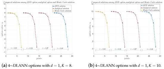
Figure 2. 4∼DLANN computational options, analytical solutions, and Monte Carlo solutions for geometric mean payoff function with $T=0.4$ and $d=1$. (a) $K=8$ and (b) $K=10$.

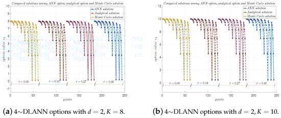
Figure 3. 4∼DLANN computational options, analytical solutions, and Monte Carlo solutions for geometric mean payoff function with $T=0.4$ and $d=2$. (a) $K=8$ and (b) $K=10$.

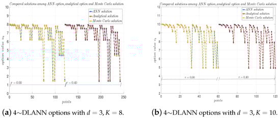
Figure 4. 4∼DLANN computational options, analytical solutions, and Monte Carlo solutions for geometric mean payoff function with $T=0.4$ and $d=3$. (a) $K=8$ and (b) $K=10$.

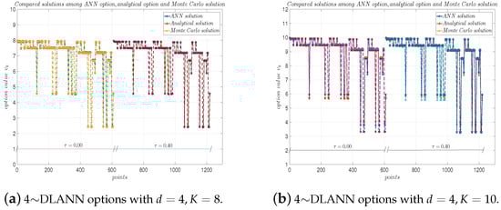
Figure 5. 4∼DLANN computational options, analytical solutions, and Monte Carlo solutions for geometric mean payoff function with $T=0.4$ and $d=4$. (a) $K=8$ and (b) $K=10$.

From Table 2, Table 3, Table 4 and Table 5, we see the absolute errors are less than $0.05$, and the relative errors are about $0.5\%$ between the 4∼DLANN solutions and analytical solutions, which illustrate that our 4∼DLANN scheme is efficient and accurate. Moreover, the results of the calculation are quite stable, and there are no unstable results. From Figure 2, Figure 3, Figure 4 and Figure 5, we see the 4∼DLANN solutions are very close to the Monte Carlo solutions and analytical solutions.

As the iteration number L increases, Figure 6 and Figure 7 record the error evolution path with respect to the training number L for different values of d. We can see from these figures that the errors are decreasing quickly as the iteration number L increases. Figure 8 records the learning rate path $\eta$. The learning rate $\eta$ fluctuates between 0 and 0.1.

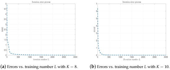
Figure 6. 4∼DLANN MSE vs. training number L with $T=0.4$ and $d=1$. (a) $K=8$ and (b) $K=10$.

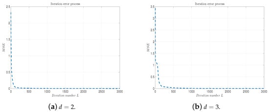
Figure 7. 4∼DLANN MSE vs. the iteration number L with $T=0.4$ and $K=8$. (a) $d=2$ and (b) $d=3$.

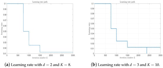
Figure 8. 4∼DLANN learning rate path with $T=0.4$. (a) $d=2$ and $K=8$; (b) $d=3$ and $K=10$.

4.3. Numerical Results with Arithmetic Mean Payoff Function

In this subsection, we list some results of the put options with arithmetic mean payoff functions

$$\mathrm{\Pi }\left(\mathit{x}\right)=max\left({\displaystyle 0,\sum _{i=1}^d{\alpha }_i{e}^{x_i}}\right).$$

(45)

This type of option has no analytical solution. We used the Monte Carlo simulation (the procedure can be seen in Algorithm 3) in order to compare the two results.

Table 6, Table 7, Table 8 and Table 9 list the results of the 4-DLANN solutions (labeled by ‘DLANN’) and the Monte Carlo simulation (labeled by ‘MC’). From these tables, we see the absolute errors (labeled by ‘ERR’) are less than $0.02$, and the relative errors (labeled by ‘RE’) are less than $0.5\%$, which illustrate that our DLANN algorithm is effective and accurate.

Table 6. Computational results of 4∼DLANN for arithmetic mean payoff function with $d=1$ and $K=8$.

Input $[\mathit{\tau },{\mathit{x}}^{\mathit{T}}]$	DLANN	MC	ERR	RE
$K=8,MSE=3.14\times {10}^{-4}$
$(0.0000,-0.3956)$	$7.3409$	$7.3267$	$0.0142$	$0.1937\%$
$(0.0000,+1.7346)$	$2.3362$	$2.3334$	$0.0028$	$0.1186\%$
$(0.1333,-0.9281)$	$7.5767$	$7.5991$	$-0.0225$	$-0.2959\%$
$(0.1333,+1.2020)$	$4.6539$	$4.6660$	$-0.0121$	$-0.2596\%$
$(0.2667,-0.9281)$	$7.5783$	$7.5937$	$-0.0154$	$-0.2027\%$
$(0.2667,+1.2020)$	$4.6694$	$4.6586$	$0.0108$	$0.2314\%$
$(0.4000,-0.9281)$	$7.5799$	$7.5882$	$-0.0083$	$-0.1095\%$
CPU time (s)	9.76	11.23

Table 7. Computational results of 4∼DLANN for arithmetic mean payoff function with $d=2$ and $K=8$.

Input $[\mathit{\tau },{\mathit{x}}^{\mathit{T}}]$	DLANN	MC	ERR	RE
$K=8,MSE=1.8\times {10}^{-3}$
$(0.0000,-2.5257,-1.0612)$	$7.7768$	$7.7870$	$-0.0102$	$-0.1308\%$
$(0.0000,-2.5257,+0.4032)$	$7.2094$	$7.2117$	$-0.0022$	$-0.0309\%$
$(0.0000,-1.0612,-2.5257)$	$7.7794$	$7.7870$	$-0.0076$	$-0.0977\%$
$(0.0000,-1.0612,-1.0612)$	$7.6579$	$7.6540$	$0.0040$	$0.0519\%$
$(0.0000,-1.0612,+0.4032)$	$7.0997$	$7.0787$	$0.0211$	$0.2979\%$
$(0.1333,-2.5257,-1.0612)$	$7.7753$	$7.7816$	$-0.0063$	$-0.0811\%$
$(0.1333,-2.5257,+0.4032)$	$7.2038$	$7.2061$	$-0.0023$	$-0.0323\%$
$(0.1333,-2.5257,+1.8677)$	$4.7199$	$4.7170$	$0.0029$	$0.0621\%$
$(0.1333,-1.0612,-2.5257)$	$7.7778$	$7.7816$	$-0.0037$	$-0.0481\%$
$(0.1333,-1.0612,-1.0612)$	$7.6537$	$7.6484$	$0.0053$	$0.0687\%$
$(0.1333,-1.0612,+0.4032)$	$7.0905$	$7.0728$	$0.0177$	$0.2497\%$
$(0.2667,-2.5257,-1.0612)$	$7.7737$	$7.7762$	$-0.0025$	$-0.0322\%$
$(0.2667,-2.5257,+0.4032)$	$7.1979$	$7.2004$	$-0.0024$	$-0.0340\%$
$(0.2667,-2.5257,+1.8677)$	$4.6962$	$4.7101$	$-0.0139$	$-0.2946\%$
$(0.2667,-1.0612,-2.5257)$	$7.7762$	$7.7761$	$0.0001$	$0.0009\%$
$(0.2667,-1.0612,-1.0612)$	$7.6493$	$7.6430$	$0.0063$	$0.0829\%$
$(0.2667,-1.0612,+0.4032)$	$7.0811$	$7.0669$	$0.0143$	$0.2019\%$
$(0.4000,-2.5257,-1.0612)$	$7.7720$	$7.7706$	$0.0013$	$0.0171\%$
$(0.4000,-2.5257,+0.4032)$	$7.1919$	$7.1944$	$-0.0025$	$-0.0347\%$
$(0.4000,-1.0612,-2.5257)$	$7.7745$	$7.7707$	$0.0037$	$0.0479\%$
$(0.4000,-1.0612,-1.0612)$	$7.6448$	$7.6373$	$0.0075$	$0.0979\%$
$(0.4000,-1.0612,+0.4032)$	$7.0717$	$7.0612$	$0.0105$	$0.1485\%$
$(0.4000,+0.4032,+0.4032)$	$6.4668$	$6.4845$	$-0.0177$	$-0.2726\%$
CPU time (s)	23.12	210.23

Table 8. Computational results of 4∼DLANN for arithmetic mean payoff function with $d=3$ and $K=8$.

Input $[\mathit{\tau },{\mathit{x}}^{\mathit{T}}]$	DLANN	MC	ERR	RE
$K=8,MSE=1.8\times {10}^{-3}$
$(0.0000,-4.6052,-4.6052,-4.6052)$	$7.9709$	$7.9900$	$-0.0191$	$-0.2396\%$
$(0.0000,-4.6052,-2.6594,-2.6594)$	$7.9468$	$7.9500$	$-0.0032$	$-0.0398\%$
$(0.0000,-2.6594,-2.6594,-4.6052)$	$7.9462$	$7.9500$	$-0.0038$	$-0.0474\%$
$(0.0000,-2.6594,-0.7136,-2.6594)$	$7.7916$	$7.7900$	$0.0015$	$0.0194\%$
$(0.0000,-0.7136,-4.6052,+1.2322)$	$6.6995$	$6.6904$	$0.0091$	$0.1358\%$
$(0.0000,+1.2322,-4.6052,-0.7136)$	$6.7042$	$6.6904$	$0.0138$	$0.2064\%$
$(0.4000,-4.6052,-4.6052,-2.6594)$	$7.9676$	$7.9540$	$0.0137$	$0.1717\%$
$(0.4000,-2.6594,-4.6052,-4.6052)$	$7.9674$	$7.9540$	$0.0134$	$0.1683\%$
$(0.4000,-2.6594,-0.7136,-0.7136)$	$7.6221$	$7.6336$	$-0.0115$	$-0.1503\%$
$(0.4000,-0.7136,+1.2322,-0.7136)$	$6.5199$	$6.5127$	$0.0072$	$0.1107\%$
$(0.4000,+1.2322,-0.7136,-4.6052)$	$6.6613$	$6.6692$	$-0.0079$	$-0.1185\%$
CPU time (s)	56.92	876.12

Table 9. Computational results of 4∼DLANN for arithmetic mean payoff function with $d=4$ and $K=8$.

Input $[\mathit{\tau },{\mathit{x}}^{\mathit{T}}]$	DLANN	MC	ERR	RE
$K=8,MSE=1.34\times {10}^{-3}$
$(0.0000,-2.0108,-2.0108,-4.6052,-2.0108)$	$7.9174$	$7.8971$	$0.0203$	$0.2575\%$
$(0.0000,-2.0108,-2.0108,-2.0108,-4.6052)$	$7.9171$	$7.8971$	$0.0200$	$0.2538\%$
$(0.0000,+0.5836,-2.0108,-4.6052,-2.0108)$	$7.4634$	$7.4824$	$-0.0190$	$-0.2544\%$
$(0.0000,+0.5836,+0.5836,-4.6052,-2.0108)$	$7.0509$	$7.0677$	$-0.0168$	$-0.2378\%$
$(0.0000,+3.1781,-4.6052,-4.6052,-2.0108)$	$1.9613$	$1.9615$	$-0.0003$	$-0.0140\%$
$(0.0000,+3.1781,-4.6052,-2.0108,-4.6052)$	$1.9618$	$1.9615$	$0.0002$	$0.0120\%$
$(0.0000,+3.1781,-2.0108,+0.5836,-4.6052)$	$1.5162$	$1.5159$	$0.0003$	$0.0209\%$
$(0.4000,-4.6052,-4.6052,+3.1781,+0.5836)$	$1.5247$	$1.5228$	$0.0019$	$0.1264\%$
$(0.4000,-2.0108,-4.6052,-4.6052,-4.6052)$	$7.9270$	$7.9430$	$-0.0159$	$-0.2006\%$
$(0.4000,-2.0108,-2.0108,-4.6052,-4.6052)$	$7.8887$	$7.9119$	$-0.0232$	$-0.2933\%$
$(0.4000,-2.0108,-2.0108,-4.6052,+0.5836)$	$7.4825$	$7.4655$	$0.0170$	$0.2279\%$
$(0.4000,-2.0108,-2.0108,+0.5836,-2.0108)$	$7.4497$	$7.4345$	$0.0152$	$0.2041\%$
$(0.4000,-2.0108,+0.5836,+0.5836,-2.0108)$	$7.0087$	$7.0192$	$-0.0105$	$-0.1501\%$
$(0.4000,+0.5836,-4.6052,-4.6052,-2.0108)$	$7.5100$	$7.4965$	$0.0135$	$0.1805\%$
$(0.4000,+0.5836,-4.6052,-4.6052,+0.5836)$	$7.0834$	$7.0813$	$0.0021$	$0.0303\%$
$(0.4000,+0.5836,-4.6052,-2.0108,-4.6052)$	$7.5000$	$7.4967$	$0.0032$	$0.0433\%$
$(0.4000,+0.5836,-4.6052,+0.5836,-2.0108)$	$7.0670$	$7.0502$	$0.0168$	$0.2383\%$
$(0.4000,+0.5836,+0.5836,-2.0108,-4.6052)$	$7.0661$	$7.0502$	$0.0159$	$0.2262\%$
$(0.4000,+3.1781,-4.6052,+0.5836,+0.5836)$	$1.0769$	$1.0765$	$0.0004$	$0.0383\%$
CPU time (s)	96.65	2913.78

Figure 9a, Figure 10a, Figure 11a and Figure 12a plot the solutions obtained by the 4-DLANN method and the Monte Carlo simulation with $T=0.4$, $d=1,2,3,4$, and $K=8$. Figure 9b, Figure 10b, Figure 11b and Figure 12b plot the errors with respect to the number of iterations L. From this figure, we see the errors decrease quickly, as the iteration number L increases.

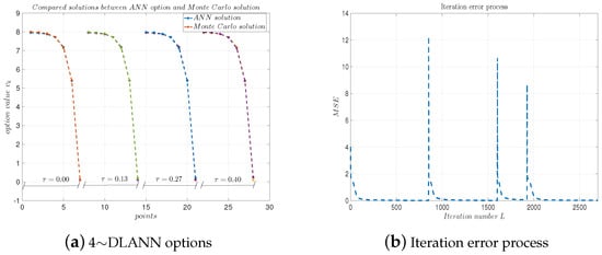
Figure 9. (a) 4∼DLANN computational options vs. Monte Carlo solutions for arithmetic mean payoff function. (b) Iteration error process. Parameters: $T=0.4,d=1$, and $K=8$.

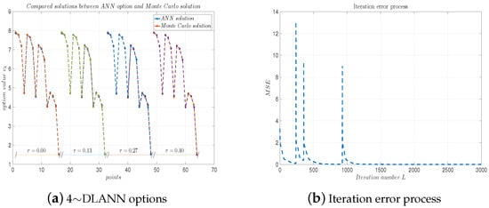
Figure 10. (a) 4∼DLANN computational options vs. Monte Carlo solutions for arithmetic mean payoff function. (b) Iteration error process. Parameters: $T=0.4,d=2$, and $K=8$.

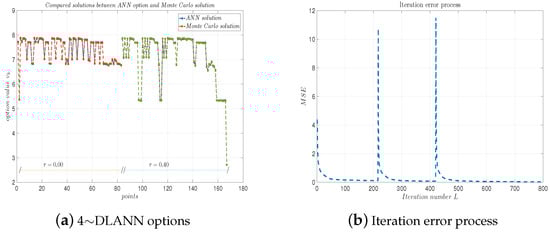
Figure 11. (a) 4∼DLANN computational options vs. Monte Carlo solutions for arithmetic mean payoff function. (b) Iteration error process. Parameters: $T=0.4,d=3$, and $K=8$.

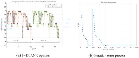
Figure 12. (a) 4∼DLANN computational options vs. Monte Carlo solutions for arithmetic mean payoff function. (b) Iteration error process. Parameters: $T=0.4,d=4$, and $K=8$.

4.4. Numerical Results with $p\ge 5$

We set the DLANN parameters as $p=5$ and $n_1=d+1,n_2=n_3=n_4=3,n_5=1$ for the arithmetic payoff functions. Table 10 lists some DLANN solutions and Monte Carlo solutions. We see the absolute errors and relative errors are less than $0.03$ and $0.3\%$, respectively. Figure 13a plots the DLANN solutions, Monte Carlo solutions, and analytical solutions for the geometric payoff functions. Figure 13b plots the errors with respect to the iteration number L. From the table and figure, we see the errors between the DLANN and MC are less than $0.3\%$, which illustrates our 5-DLANN is more efficient than the $p\le 4$.

Table 10. Computational results of 5∼DLANN for arithmetic mean payoff function with $d=2$ and $K=8$.

Input $[\mathit{\tau },{\mathit{x}}^{\mathit{T}}]$	DLANN	MC	ERR	RE
$K=8,MSE=1.8\times {10}^{-3}$
$(0.0000,-4.6052,-1.4919)$	$7.8603$	$7.8825$	$-0.0223$	$-0.2825\%$
$(0.0000,-3.0485,-1.4919)$	$7.8644$	$7.8638$	$0.0006$	$0.0076\%$
$(0.0000,-3.0485,+1.6214)$	$5.4566$	$5.4462$	$0.0104$	$0.1905\%$
$(0.0000,-1.4919,-4.6052)$	$7.8746$	$7.8825$	$-0.0079$	$-0.1007\%$
$(0.0000,-1.4919,-3.0485)$	$7.8779$	$7.8638$	$0.0141$	$0.1790\%$
$(0.0000,+0.0648,-3.0485)$	$7.4619$	$7.4428$	$0.0191$	$0.2563\%$
$(0.4000,-4.6052,-1.4919)$	$7.8610$	$7.8664$	$-0.0054$	$-0.0691\%$
$(0.4000,-4.6052,+1.6214)$	$5.4366$	$5.4441$	$-0.0075$	$-0.1374\%$
$(0.4000,-3.0485,-1.4919)$	$7.8649$	$7.8476$	$0.0173$	$0.2207\%$
$(0.4000,-3.0485,+0.0648)$	$7.4096$	$7.4258$	$-0.0162$	$-0.2187\%$
$(0.4000,-1.4919,-4.6052)$	$7.8722$	$7.8663$	$0.0058$	$0.0739\%$
$(0.4000,+0.0648,-3.0485)$	$7.4187$	$7.4259$	$-0.0072$	$-0.0976\%$
CPU time (s)	29.23	276.45

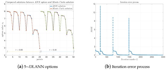
Figure 13. (a) 5∼DLANN computational options vs. Monte Carlo solutions for geometric mean payoff function. (b) Iteration error process. Parameters: $T=0.4,d=2$, and $K=8$.

Figure 14 plots the $6\sim$ DLANN solutions and the errors’ evolution process with respect to the iteration number L under the parameters $n_1=d+1,n_2=n_3=n_4=3,n_5=2,n_6=1$ for arithmetic payoff functions. Again, these numerical results confirm our $p\sim$ DLANN is more accurate and efficient for $p\ge 5$.

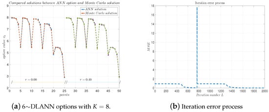
Figure 14. (a) 6∼DLANN computational options vs. Monte Carlo solutions for arithmetic mean payoff function. (b) Iteration error process. Parameters: $T=0.4,d=2$, and $K=8$.

Compared with $p=3,4$ the computational results of the DLANN with $p=5,6$ are more accurate, which illustrate that our $p\sim$ DLANN is convergent with respect to the ANN layers p.

4.5. Numerical Results for $p\sim$ TSDLANN

Using p-TSDLANN, as shown in Algorithm 2, we computed the options with geometric payoff functions. Figure 15 plots the $p\sim$ TSDLANN solutions with $p=4,M=2,$$T=0.4$, compared with the analytical solutions and Monte Carlo solutions, from which we see the p-TSDLANN solutions are very close to the analytical solutions. The experiments show, with the same accuracy, the CPU time of this Algorithm is about half of that computed by the p-DLANN.

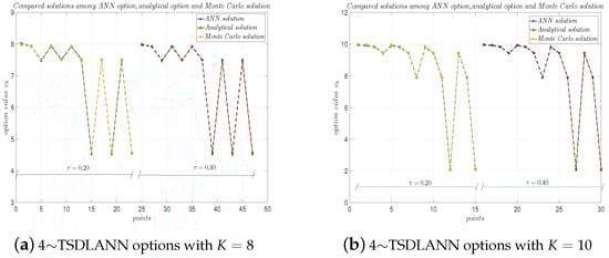
Figure 15. 4∼TSDLANN computational options, analytical solutions, and Monte Carlo solutions for geometric mean payoff function with $T=0.4,d=2$. (a) $K=8$ and (b) $K=10$.

5. Conclusions

This paper introduces a $p$-layers deep learning ANN to price European multi-asset options based on the discrete PDE. By setting the numbers $(n_1,n_2,\dots ,n_p)$ of the DLANN structure, the multi-asset options are simulated correctly and efficiently. The key point is obtaining the discrete formula of the PDE that is established by the option valuation and then computing the gradients of the $p\sim$ DLANN with respect to the net weights ${\mathit{\omega }}^{(\ell )}$ and net bias ${\mathit{\theta }}^{(\ell )}$. By setting the learning parameter $\eta$, the $p\sim$ DLANN is trained well, and the optimal parameters ${\mathit{\omega }}^{(\ell )}$ and ${\mathit{\theta }}^{(\ell )}$ are obtained. Lastly, the option prices are simulated by inputting the asset log prices $\mathit{x}$ and remainder time $\tau$ into the trained $p\sim$ DLANN.

Numerical examples are provided for geometric mean payoff functions and arithmetic mean payoff functions. These examples show that the p-layers DLANN has a powerful capability for multi-asset European option pricing. The relative errors of the $p\sim$ DLANN options are less than $0.5\%$, and this calculation accuracy is comparable to the Monte Carlo simulation. Moreover, we propose a so-called $p\sim$ TSDLANN, which improves the accuracy and saves CPU time.

In the future, we will prove the convergence of $p\sim$ DLANN under certain conditions. The challenge is how to analyze the errors between the actual options and computed options by $p\sim$ DLANN. Moreover, we will consider applying the $p\sim$ DLANN to more complex options, such as multi-asset American options, multi-asset Asian options, and multi-asset barrier options, which is somewhat complicated.

Appendix A.1. Deducing the Derivatives for Weights ${\mathit{\omega }}_{IJ}^{(\ell )}$ and Bias ${\mathit{\theta }}_I^{(\ell )}$

Appendix A.1.1. Deducing the Derivatives for Weights ${\mathit{\omega }}_{IJ}^{(\ell )}$

The partial derivatives of ${\displaystyle \frac{\partial U_1^{(p,k)}}{\partial {\omega }_{1J}^{\left(p\right)}}}$ are

$$\begin{array}{c}\hfill {\displaystyle \frac{\partial U_1^{(p,k)}}{\partial {\omega }_{1J}^{\left(p\right)}}}=f^{\prime }\left(O_1^{\left(p\right)}\right){\displaystyle \frac{\partial O_1^{(p,k)}}{\partial {\omega }_{1J}^{\left(p\right)}}}=f^{\prime }\left(O_1^{\left(p\right)}\right){\displaystyle \frac{\partial }{\partial {\omega }_{1J}^{\left(p\right)}}}\sum _{j=1}^{n_{p-1}}{\omega }_{1j}^{\left(p\right)}{U}_j^{(p-1)}=U_J^{(p-1,k)},\end{array}$$

(A1)

for $J=1,2,\dots ,n_{p-1}$. The partial derivatives of ${\displaystyle \frac{\partial U_1^{(p,k)}}{\partial {\omega }_{IJ}^{(p-1)}}}$ are

$$\begin{array}{ccc}\hfill {\displaystyle \frac{\partial U_1^{(p,k)}}{\partial {\omega }_{IJ}^{(p-1)}}}& =& f^{\prime }\left(O_1^{\left(p\right)}\right){\displaystyle \frac{\partial }{\partial {\omega }_{IJ}^{(p-1)}}}\sum _{j=1}^{n_{p-1}}{\omega }_{ij}^{\left(p\right)}{U}_j^{(p-1)},\hfill \\ & =& f^{\prime }\left(O_1^{\left(p\right)}\right){\displaystyle \frac{\partial }{\partial {\omega }_{IJ}^{(p-1)}}}\sum _{j=1}^{n_{p-1}}{\omega }_{1j}^{\left(p\right)}{f}^{\prime }\left(O_j^{(p-1,k)}\right)\sum _{\ell =1}^{n_{p-2}}{\omega }_{j\ell }^{(p-1)}{U}_{\ell }^{(p-2)},\hfill \\ & =& {\omega }_{1I}^{\left(p\right)}g\left(U_I^{(p-1,k)}\right)U_J^{(p-2,k)},\hfill \end{array}$$

(A2)

for $I=1,2,\dots ,n_{p-1}$ and $J=1,2\dots ,n_{p-2}$. Similarly, we have

$$\begin{array}{c}\hfill {\displaystyle \frac{\partial U_1^{(p,k)}}{\partial {\omega }_{IJ}^{(p-2)}}=g\left(U_I^{(p-2,k)}\right)U_J^{(p-3,k)}\sum _{j=1}^{n_{p-1}}{\omega }_{1j}^{\left(p\right)}{\omega }_{jI}^{(p-1)}g\left(U_j^{(p-1,k)}\right),}\end{array}$$

(A3)

for $I=1,2,\dots ,n_{p-2}$ and $J=1,2\dots ,n_{p-3}$.

$$\begin{array}{c}\hfill {\displaystyle \frac{\partial U_1^{(p,k)}}{\partial {\omega }_{IJ}^{(p-3)}}}=g\left(U_I^{(p-3,k)}\right)U_J^{(p-4,k)}\sum _{j_1=1}^{n_{p-1}}{\omega }_{1j_1}^{\left(p\right)}g\left(U_{j_1}^{(p-1,k)}\right)\sum _{j_2=1}^{n_{p-2}}{\omega }_{j_1{j}_2}^{(p-1)}g\left(U_{j_2}^{(p-2,k)}\right){\omega }_{j_{2}I}^{(p-2)},\end{array}$$

(A4)

for $I=1,2,\dots ,n_{p-3}$ and $J=1,2\dots ,n_{p-4}$.

$$\begin{array}{ccc}\hfill {\displaystyle \frac{\partial U_1^{(p,k)}}{\partial {\omega }_{IJ}^{(p-\ell )}}}& =& g\left(U_I^{(p-\ell ,k)}\right)U_J^{(p-(\ell +1),k)}\sum _{j_1=1}^{n_{p-1}}{\omega }_{1j_1}^{\left(p\right)}g\left(U_{j_1}^{(p-1,k)}\right)\sum _{j_2=1}^{n_{p-2}}{\omega }_{j_1{j}_2}^{(p-1)}g\left(U_{j_2}^{(p-2,k)}\right)\cdots \cdots \hfill \\ & & \sum _{j_{\ell -1}=1}^{n_{p-(\ell -1)}}{\omega }_{j_{\ell -2}{j}_{\ell -1}}^{(p-(\ell -2\left)\right)}g\left(U_{j_{\ell -1}}^{(p-(\ell -1),k)}\right){\omega }_{j_{\ell -1}I}^{(p-(\ell -1\left)\right)},\hfill \end{array}$$

(A5)

for $I=1,2,\dots ,n_{p-\ell }$, $J=1,2,\dots ,n_{p-\ell -1}$, and $\ell =0,1,\cdots ,p-2$, with the function

$$\begin{array}{c}\hfill g\left(U\right)=U(1-U).\end{array}$$

(A6)

Appendix A.1.2. Deducing the Derivatives for Weights ${\mathit{\theta }}_I^{(\ell )}$

The derivatives of $\partial U_1^{(p,k)}/\partial {\theta }_1^{\left(p\right)}$ are

$$\begin{array}{c}\hfill {\displaystyle \frac{\partial U_1^{(p,k)}}{\partial {\theta }_1^{\left(p\right)}}}=f^{\prime }\left(O_1^{\left(p\right)}\right){\displaystyle \frac{\partial O_1^{(p,k)}}{\partial {\theta }_1^{\left(p\right)}}}=f^{\prime }\left(O_1^{\left(p\right)}\right){\displaystyle \frac{\partial }{\partial {\theta }_1^{\left(p\right)}}}\left(\sum _{i=1}^{n_{p-1}}{\omega }_{1i}^{\left(p\right)}{U}_i^{(p-1)}+{\theta }_1^{\left(p\right)}\right)=1,\end{array}$$

(A7)

for $I=1,2,\dots ,n_p$. The derivatives are $\partial U_1^{(p,k)}/\partial {\theta }_I^{(p-1)}$ is

$$\begin{array}{ccc}\hfill {\displaystyle \frac{\partial U_1^{(p,k)}}{\partial {\theta }_I^{(p-1)}}}& =& f^{\prime }\left(O_1^{(p,k)}\right){\displaystyle \frac{\partial }{\partial {\theta }_I^{(p-1)}}}\sum _{j=1}^{n_{p-1}}{\omega }_{1j}^{\left(p\right)}{U}_j^{(p-1,k)}\hfill \\ & =& f^{\prime }\left(O_1^{(p,k)}\right){\displaystyle \frac{\partial }{\partial {\theta }_I^{(p-1)}}}\sum _{j=1}^{n_{p-1}}{\omega }_{1j}^{\left(p\right)}{f}^{\prime }\left(O_j^{(p-1,k)}\right)\left(\sum _{\ell =1}^{n_{p-2}}{\omega }_{j\ell }^{(p-1)}{U}_{\ell }^{(p-2,k)}+{\theta }_j^{(p-1)}\right)\hfill \\ & =& {\omega }_{1I}^{\left(p\right)}g\left(U_I^{(p-1,k)}\right),\hfill \end{array}$$

(A8)

for $I=1,2,\dots ,n_{p-1}$. Similarly, we have

$$\begin{array}{c}\hfill {\displaystyle \frac{\partial U_1^{(p,k)}}{\partial {\theta }_I^{(p-2)}}=\sum _{j=1}^{n_{p-1}}{\omega }_{1j}^{\left(p\right)}g\left(U_j^{(p-1,k)}\right){\omega }_{jI}^{(p-1)}g\left(U_I^{(p-2,k)}\right),}\end{array}$$

(A9)

for $I=1,2,\dots ,n_{p-2}$. The derivatives of $\partial U_1^{(p,k)}/\partial {\theta }_I^{(p-3)}$ are

$$\begin{array}{c}\hfill {\displaystyle \frac{\partial U_1^{(p,k)}}{\partial {\theta }_I^{(p-3)}}=\sum _{j_1=1}^{n_{p-1}}{\omega }_{1j_1}^{\left(p\right)}g\left(U_{j_1}^{(p-1,k)}\right)\sum _{j_2=1}^{n_{p-2}}{\omega }_{j_1{j}_2}^{(p-1)}g\left(U_{j_2}^{(p-2,k)}\right){\omega }_{j_{2}I}^{(p-2)}g\left(U_I^{(p-3,k)}\right),}\end{array}$$

(A10)

for $I=1,2,\dots ,n_{p-3}$. The derivatives of $\partial U_1^{(p,k)}/\partial {\theta }_I^{(p-\ell )}$ are

$$\begin{array}{c}\hfill {\displaystyle \frac{\partial U_1^{(p,k)}}{\partial {\theta }_I^{(p-\ell )}}=\sum _{j_1=1}^{n_{p-1}}{\omega }_{1j_1}^{\left(p\right)}g\left(U_{j_1}^{(p-1,k)}\right)\sum _{j_2=1}^{n_{p-2}}{\omega }_{j_1{j}_2}^{(p-1)}g\left(U_{j_2}^{(p-2,k)}\right)\cdots \cdots \sum _{j_{\ell -1}=1}^{n_{p-(\ell -1)}}{\omega }_{j_{\ell -2}{j}_{\ell -1}}^{(p-(\ell -2\left)\right)}}\\ \hfill ·g\left(U_{j_{\ell -1}}^{(p-(\ell -1),k)}\right){\omega }_{j_{\ell -1}I}^{(p-(\ell -1\left)\right)}g\left(U_I^{(p-\ell ,k)}\right),\end{array}$$

(A11)

for $I=1,2,\dots ,n_{p-\ell },\ell =0,1,\dots ,p-2$.

Appendix A.2. Deducing g ′ (U) and g ′′ (U)

The function $g\left(U\right)$ is

$$\begin{array}{c}\hfill g\left(U\right)={\displaystyle \frac{1}{1+e^{-U}}}.\end{array}$$

(A12)

So, the derivative $g^{\prime }\left(U\right)$ is

$$\begin{array}{c}\hfill g^{\prime }\left(U\right)={\displaystyle \frac{1}{{(1+e^{-U})}^2}}{e}^{-U}=g\left(U\right)\left(1-g\left(U\right)\right),\end{array}$$

(A13)

and the second derivative $g^{″}\left(U\right)$ is

$$\begin{array}{c}\hfill g^{\prime \prime }\left(U\right)=g^{\prime }\left(U\right)(1-g\left(U\right))-g\left(U\right)g^{\prime }\left(U\right)=g\left(U\right)(1-g\left(U\right)(1-2g\left(U\right)).\end{array}$$

(A14)

References

- Álvarez, D.; González-Rodríguez, P.; Kindelan, M. A local radial basis function method for the Laplace-Beltrami operator. J. Sci. Comput. 2021, 86, 28. [Google Scholar] [CrossRef]
- Banei, S.; Shanazari, K. On the convergence analysis and stability of the RBF-adaptive method for the forward-backward heat problem in 2D. Appl. Numer. Math. 2021, 159, 297–310. [Google Scholar] [CrossRef]
- Bastani, A.F.; Ahmadi, Z.; Damircheli, D. A radial basis collocation method for pricing American options under regime-switching jump-diffusion models. Appl. Numer. Math. 2013, 65, 79–90. [Google Scholar] [CrossRef]
- Bollig, E.; Flyer, N.; Erlebacher, G. Solution to PDEs using radial basis function finite-differences (RBF-FD) on multiple GPUs. J. Comput. Phys. 2012, 231, 7133–7151. [Google Scholar] [CrossRef]
- Fornberg, B.; Lehto, E. Stabilization of RBF-generated finite difference methods for convective PDEs. J. Comput. Phys. 2011, 230, 2270–2285. [Google Scholar] [CrossRef]
- Fornberg, B.; Piret, C. A stable algorithm for at radial basis functions on a sphere. SIAM J. Sci. Comput. 2007, 30, 60–80. [Google Scholar] [CrossRef]
- Fornberg, B.; Piret, C. On choosing a radial basis function and a shape parameter when solving a convective PDE on a sphere. J. Comput. Phys. 2008, 227, 2758–2780. [Google Scholar] [CrossRef]
- Larsson, E.; Shcherbakov, V.; Heryudono, A. A least squares radial basis function partition of unity method for solving PDEs. SIAM J. Sci. Comput. 2017, 39, 2538–2563. [Google Scholar] [CrossRef]
- Li, H.G.; Mollapourasl, R.; Haghi, M. A local radial basis function method for pricing options under the regime switching model. J. Sci. Comput. 2019, 79, 517–541. [Google Scholar] [CrossRef]
- Shcherbakov, V.; Larsson, E. Radial basis function partition of unity methods for pricing vanilla Basket options. Comput. Math. Appl. 2016, 71, 185–200. [Google Scholar] [CrossRef]
- Sunday, E.; Olabisi, U.; Enahoro, O. Analytical solutions of the Black–Scholes pricing model for European option valuation via a projected differential transformation method. Entropy 2015, 17, 7510–7521. [Google Scholar] [CrossRef]
- Zhao, W.J. An artificial boundary method for American option pricing under the CEV model. SIAM J. Numer. Anal. 2008, 46, 2183–2209. [Google Scholar]
- Chiarella, C.; Kang, B.; Meyer, G.H. The numerical solution of the American option pricing problem-finite difference and transform approaches. World Sci. Books 2014, 127, 161–168. [Google Scholar]
- in’t Hout, K.; Foulon, S. ADI finite difference schemes for option pricing in the Heston model with correlation. Int. J. Numer. Anal. Model. 2008, 7, 303–320. [Google Scholar]
- in ’t Hout, K.; Weideman, J.A.C. A contour integral method for the Black–Scholes and Heston equations. SIAM J. Sci. Comput. 2011, 33, 763–785. [Google Scholar] [CrossRef]
- Pang, H.; Sun, H. Fast numerical contour integral method for fractional diffusion equations. J. Sci. Comput. 2016, 66, 41–66. [Google Scholar] [CrossRef]
- Song, L.; Wang, W. Solution of the fractional Black-Scholes option pricing model by finite difference method. Abstr. Appl. Anal. 2013, 2013, 194286. [Google Scholar] [CrossRef]
- Gabriel, T.A.; Amburgey, J.D.; Bishop, B.L. CALOR: A Monte Carlo Program Package for the Design and Analysis of Calorimeter Systems. 2024, In FORTRAN IV, osti Information Bridge Server. Available online: https://www.osti.gov/servlets/purl/7215451/ (accessed on 13 December 2024).
- Gamba, A. An Extension of Least Squares Monte Carlo Simulation for Multi-Options Problems; 2002. pp. 1–40. Available online: https://www.realoptions.org/papers2002/Gamba.pdf (accessed on 13 December 2024).
- Rodriguez, A.L.; Grzelak, L.A.; Oosterlee, C.W. On an efficient multiple time-step Monte Carlo simulation of the SABR model. Soc. Sci. Electron. Publ. 2016, 17, 1549–1565. [Google Scholar] [CrossRef][Green Version]
- Ma, J.; Zhou, Z. Convergence analysis of iterative Laplace transform methods for the coupled PDEs from regime-switching option pricing. J. Sci. Comput. 2018, 75, 1656–1674. [Google Scholar] [CrossRef]
- Ma, J.; Zhou, Z. Fast Laplace transform methods for the PDE system of Parisian and Parasian option pricing. Sci. China Math. 2022, 65, 1229–1246. [Google Scholar] [CrossRef]
- Panini, R.; Srivastav, R.P. Option pricing with Mellin transforms. Math. Comput. Model. 2004, 40, 43–56. [Google Scholar] [CrossRef]
- Zhou, Z.; Ma, J.; Sun, H. Fast Laplace transform methods for free-boundary problems of fractional diffusion equations. J. Sci. Comput. 2018, 74, 49–69. [Google Scholar] [CrossRef]
- Zhou, Z.; Xu, W. Robust willow tree method under Lévy processes. J. Comput. Appl. Math. 2023, 424, 114982. [Google Scholar] [CrossRef]
- Zhou, Z.; Xu, W. Joint calibration of S&P 500 and VIX options under local stochastic volatility models. Int. J. Financ. Econ. 2024, 29, 273–310. [Google Scholar]
- Anderson, D.; Ulrych, U. Accelerated American option pricing with deep neural networks. Quant. Financ. Econ. 2023, 7. [Google Scholar] [CrossRef]
- Carverhill, A.P.; Cheuk, T.H.F. Alternative Neural Network Approach for Option Pricing and Hedging; Social Science Electronic Publishing: Rochester, NY, USA, 2024; pp. 1–17. [Google Scholar] [CrossRef]
- Gan, L.; Liu, W. Option pricing based on the residual neural network. Comput. Econ. 2023, 63, 1327–1347. [Google Scholar] [CrossRef]
- Kapllani, L.; Teng, L. Deep learning algorithms for solving high-dimensional nonlinear backward stochastic differential equations. Discret. Contin. Dyn. Syst. Ser. B 2024, 29, 1695–1729. [Google Scholar] [CrossRef]
- Lee, Y.; Son, Y. Predicting arbitrage-free American option prices using artificial neural network with pseudo inputs. Ind. Eng. Manag. Syst. 2021, 20, 119–129. [Google Scholar] [CrossRef]
- Mary, M.; Salchenberger, L. A neural network model for estimating option prices. Appl. Intell. 1993, 3, 193–206. [Google Scholar]
- Nikolas, N.; Lorenz, R. Interpolating Between BSDEs and PINNs: Deep Learning, for Elliptic and Parabolic Boundary Value Problems. J. Mach. Learn. 2024, 2, 31–64. [Google Scholar] [CrossRef]
- Balkin, R.; Ceniceros, H.D.; Hu, R. Stochastic Delay Differential Games: Financial Modeling and Machine Learning Algorithms. J. Mach. Learn. 2024, 3, 23–63. [Google Scholar] [CrossRef]
- Teng, Y.; Li, Y.; Wu, X. Option volatility investment strategy: The combination of neural network and classical volatility prediction model. Discret. Dyn. Nat. Soc. 2022, 2022, 8952996. [Google Scholar] [CrossRef]
- Tung, W.L.; Quek, C. Financial volatility trading using a self-organising neural-fuzzy semantic network and option straddle-based approach. Expert Syst. Appl. 2011, 38, 4668–4688. [Google Scholar] [CrossRef]
- Umeorah, N.; Mashele, P.; Agbaeze, O.M.J.C. Barrier Options and Greeks: Modeling with Neural Networks. Axioms 2023, 12, 384. [Google Scholar] [CrossRef]
- Wang, H. Nonlinear neural network forecasting model for stock index option price: Hybrid GJRCGARCH approach. Expert Syst. Appl. 2009, 36, 564–570. [Google Scholar] [CrossRef]
- Zhou, Z.; Wu, H.; Li, Y.; Kang, C.; Wu, Y. Three-layer artificial neural network for pricing multi-asset European option. Mathematics 2024, 12, 2770. [Google Scholar] [CrossRef]
- Jiang, L. Mathematical Models and Methods of Option Pricing (Chinese Edition); Higher Education Press: Beijing, China, 2008. [Google Scholar]
Disclaimer/Publisher’s Note: The statements, opinions and data contained in all publications are solely those of the individual author(s) and contributor(s) and not of MDPI and/or the editor(s). MDPI and/or the editor(s) disclaim responsibility for any injury to people or property resulting from any ideas, methods, instructions or products referred to in the content. |
© 2025 by the authors. Licensee MDPI, Basel, Switzerland. This article is an open access article distributed under the terms and conditions of the Creative Commons Attribution (CC BY) license (https://creativecommons.org/licenses/by/4.0/).