Variable Selection for Generalized Single-Index Varying-Coefficient Models with Applications to Synergistic G × E Interactions

Abstract

Complex diseases such as type 2 diabetes are influenced by both environmental and genetic risk factors, leading to a growing interest in identifying gene–environment (G × E) interactions. A three-step variable selection method for single-index varying-coefficients models was proposed in recent research. This method selects varying and constant-effect genetic predictors, as well as non-zero loading parameters, to identify genetic factors that interact linearly or nonlinearly with a mixture of environmental factors to influence disease risk. In this paper, we extend this approach to a binary response setting given that many complex human diseases are binary traits. We also establish the oracle property for our variable selection method, demonstrating that it performs as well as if the correct sub-model were known in advance. Additionally, we assess the performance of our method through finite-sample simulations with both continuous and discrete gene variables. Finally, we apply our approach to a type 2 diabetes dataset, identifying potential genetic factors that interact with a combination of environmental variables, both linearly and nonlinearly, to influence the risk of developing type 2 diabetes.

1. Introduction

The identification of gene–environment (G × E) interactions for complex traits has been a longstanding challenge in genetic studies. Ottman [1] defined G × E interaction as “different effect of a genotype on disease risk in persons with different environmental exposures”. Traditionally, G × E interactions have been studied using a single environmental factor, as incorporating multiple environmental factors exponentially increases model complexity. This can lead to biased estimates and large standard errors, a phenomenon known as the curse of dimensionality. Moreover, an increasing number of epidemiological studies have shown that disease risk can be influenced by simultaneous exposure to multiple environmental factors [2,3]. However, little is known about how multiple environmental factors, when considered collectively, interact with genetic factors to affect disease outcomes. Investigating this area could provide valuable insights and inform strategies for future disease prevention.

Guan et al. [4] proposed a single-index varying-coefficients model in the form $Y={\sum }_{k=0}^p{m}_k\left(\mathit{X}\mathit{\beta }\right){\mathit{G}}_k+\mathbf{ϵ}$ to address non-linear gene–environment interactions. However, this model is limited to continuous phenotypes. In this paper, we generalize the model to handle binary phenotype data, given that many complex human diseases are binary traits in nature. Specifically, we propose a generalized single-index varying-coefficients model (gSIVCM):

$$log\left(P(Y=1|\mathit{X},\mathit{G})/P(Y=0|\mathit{X},\mathit{G})\right)=\sum _{k=0}^p{m}_k\left(\mathit{X}\mathit{\beta }\right){\mathit{G}}_k$$

(1)

where $m_k(·),k=0,1,\dots ,p$ represents the unknown gene effect of ${\mathit{G}}_k$, modeled as a non-parametric function modulated by its loading index $\mathit{X}\mathit{\beta }$. Here, X represents q-dimensional environmental exposures, and $u=\mathit{X}\mathit{\beta }$ captures the joint effect of q environmental factors. The effect of these factors on the response is modeled through the $m_k(·)$ function. In this model, we allow the effect of ${\mathit{G}}_k$ on the risk of Y to vary across multiple X through the $m_k(·)$ function.

If $m_k\left(u\right)=0$, then ${\mathit{G}}_k$ has no effect on Y. If $m_k\left(u\right)=\alpha$, where $\alpha$ is a constant, the effect of ${\mathit{G}}_k$ on Y is constant, and there is no interaction between ${\mathit{G}}_k$ and the mixture of X. If $m_k\left(u\right)\ne \alpha$, we conclude that ${\mathit{G}}_k$ interacts with the environmental mixture, and the form of the interaction effect is captured by the non-parametric function $m_k(·)$.

The unique structure of gSIVCM enables us to capture how a mixture of multiple environmental factors interacts with genetic factors. Moreover, model (1) is highly flexible and can accommodate a wide range of models. For example, when $q=1$ and $\beta =1$, it reduces to a generalized varying-coefficients model; when $p=1$ and $\mathit{G}=\mathbf{1}$, it becomes a standard generalized single-index model.

When both the number of gene variables and the number of environmental variables X is large, the complexity of model (1) introduces unique challenges for variable selection, particularly due to the nonlinear, non-parametric structure of the function $m_k(·)$ and its unknown loading parameter $\mathit{\beta }$. Guan et al. [4] recently proposed a three-step variable selection approach for single-index varying-coefficients model (SIVCM), which classifies the non-parametric gene effect into varying, constant, and zero effects, while also identifying non-zero loading parameters. In this paper, we extend this variable selection approach to gSIVCM. Instead of penalizing the squared error loss as in SIVCM, we implement a penalized log-likelihood method tailored to our model.

Variable selection has been a central topic in modern statistical research. The core idea is to add a penalty term to the optimization function. Different choices of penalty functions yield estimators with varying properties. Fan and Li [5] introduced three key criteria for a penalized estimator: sparsity, unbiasedness, and continuity. They also characterized the oracle property, which ensures that the model can (1) consistently identify the true subset of relevant variables and (2) estimate their coefficients as accurately as if the true model were known in advance. This has become a benchmark for evaluating new penalized estimators. Examples of penalized functions include Bridge regression [6], the Least Absolute Shrinkage and Selection Operator (LASSO) [7], Adaptive LASSO [8], Smoothly Clipped Absolute Deviation (SCAD) [5], and Minimax Concave Penalty (MCP) [9]. While LASSO is well-regarded for its simple formulation and efficient algorithm (e.g., LARS), it does not possess the oracle property. In contrast, Adaptive LASSO, SCAD, and MCP all satisfy the oracle property. For our model, we chose the MCP penalty due to its desirable theoretical and practical properties.

The rest of the paper is organized as follows: Section 2 introduces the proposed variable selection method, including the formulation of the penalized log-likelihood, the iterative optimization procedure, and the selection of tuning parameters and initial values for $\mathit{\beta }$. Section 3 discusses the asymptotic properties of the proposed method. In Section 4, we evaluate the performance of our method through several finite-sample simulations. Finally, in Section 5, we apply our method to a type 2 diabetes dataset, followed by conclusion and discussion.

2. Statistical Method

Throughout the paper, superscript T is used to denote matrix transpose, $\left|\right|·{\left|\right|}_p$ is used to denote $L_p$ norm, $log\left(a\right)$ is used to denote the natural logarithm of a. For notation simplicity, $\left|\right|·\left|\right|$ denotes the $L_2$ norm throughout the paper. For the sake of simplicity, we use constant and non-zero constant interchangeably.

2.1. Model Setup

The generalized single-index varying-coefficients model for the binary case is set as follows:

$$log\left(P(\mathit{Y}=1|\mathit{X},\mathit{G})/P(\mathit{Y}=0|\mathit{X},\mathit{G})\right)=\sum _{k=0}^p{m}_k\left(\mathit{X}\mathit{\beta }\right){\mathit{G}}_k$$

where ${\mathit{Y}}_{n\times 1}={(Y_1,Y_2,\dots ,Y_n)}^T$ represents the binary response variable, and n denotes the sample size. The set ${\left\{m_k(.)\right\}}_{k=0,1,\dots ,p}$ comprises $p+1$ unknown real-valued continuous functions. ${\mathit{X}}_{n\times q}=({\mathit{X}}_1,{\mathit{X}}_2,\dots ,{\mathit{X}}_q)$ contains environmental variables, and ${\mathit{\beta }}_{q\times 1}={({\beta }_1,\dots ,{\beta }_q)}^T$ represents the loading parameters of the model. ${\mathit{G}}_{n\times (p+1)}=({\mathit{G}}_0,{\mathit{G}}_1,\dots ,{\mathit{G}}_p)$ where ${\mathit{G}}_0={(1,\dots ,1)}^T$ and ${\mathit{G}}_k={(G_{1k},G_{2k},\dots ,G_{nk})}^T$ is a continuous or discrete vector of length n for $k=1,2,\dots p$. Consequently, for $k\ne 0$, $m_k\left(\mathit{X}\mathit{\beta }\right)$ represents the effect of ${\mathit{G}}_k$ on Y on a log-odds scale, while $m_0\left(\mathit{X}\mathit{\beta }\right)$ serves as the intercept term.

For simplicity of notation, we denote $\mathit{\mu }={\sum }_{k=0}^p{m}_k\left(\mathit{X}\mathit{\beta }\right){\mathit{G}}_k$. Thus, model (1) can be rewritten as follows:

$$log\left(P(Y=1|\mathit{X},\mathit{G})/P(Y=0|\mathit{X},\mathit{G})\right)=\mathit{\mu }$$

(2)

2.2. Estimation Method

Our goal is to estimate and select unknown functions ${\left\{m_k(.)\right\}}_{k=0,1,\dots ,p}$ and unknown loading parameter $\mathit{\beta }={({\beta }_1,\dots ,{\beta }_q)}^T$. For the sake of identifiability, we assume ${\left|\right|\mathit{\beta }\left|\right|}_2=1$, ${\beta }_1>0$, and that $m_k(.)$ cannot take the form $m_j\left(\mathit{u}\right)={\mathbf{\alpha }}^T\mathit{u}{\mathit{\beta }}^T\mathit{u}+{\mathit{\gamma }}^T\mathit{u}+c$.

We first approximate the non-parametric function $m_k\left(u\right)$ with B-spline basis functions. Without loss of generality, we assume $u\in [0,1]$, denote K as the number of internal knots and h as the degree of the B-spline basis function. For instance, $h=1$ indicates linear splines, $h=2$ represents quadratic splines, and $h=3$ represents cubic splines. From standard B-spline theory, let $u_1,u_2,\dots ,u_K$ be internal knots satisfying $0=u_0\le u_1<u_2<\dots <u_K<u_{K+1}=1$, and let $I_{n_t}$ be the left-closed, right-open interval $[u_{t-1},u_t)$ for $1\le t\le K$, and $I_{n_{K+1}}$ the closed interval $[u_K,u_{K+1}]$. Let $\mathcal{F}$ be a collection of functions f defined on $[0,1]$ satisfying: (i) the restriction of f to $I_{n_t}$ is a polynomial of degree h or less for $1\le t\le K+1$; (ii) f is $h-1$ times continuously differentiable on $[0,1]$.

Let $L=K+h+1$. Then, by Schumaker [10], we have a normalized B-spline basis function $\tilde{\mathit{B}}\left(u\right)=(\widetilde{{\mathit{B}}_1}\left(u\right),\widetilde{{\mathit{B}}_2}\left(u\right),\dots ,\widetilde{{\mathit{B}}_L}\left(u\right))$ for $\mathcal{F}$. There exists a linear transformation matrix $\mathbf{\Pi }$ such that

$$\mathbf{\Pi }\tilde{\mathit{B}}\left(u\right)=\left(\mathbf{1},\overline{\mathit{B}}\left(u\right)\right)=\left(\mathbf{1},{\mathit{B}}_2\left(u\right),{\mathit{B}}_3\left(u\right),\dots ,{\mathit{B}}_L\left(u\right)\right)=\mathit{B}\left(u\right),$$

where each component of $\overline{\mathit{B}}\left(u\right)$ is a function of u. Then, for $0\le k\le p$, we approximate $m_k\left(u\right)$ by

$$m_k\left(u\right)\approx (1,B_2\left(u\right),B_3\left(u\right),\dots ,B_L\left(u\right))·{({\gamma }_{k1},{\gamma }_{k2},\dots ,{\gamma }_{kL})}^T=\mathit{B}\left(u\right){\mathit{\gamma }}_k={\gamma }_{k1}+\overline{\mathit{B}}\left(u\right){\mathit{\gamma }}_{k\ast },$$

(3)

where ${\mathit{\gamma }}_{k\ast }={({\gamma }_{k2},{\gamma }_{k3},\dots ,{\gamma }_{kL})}^T$ and ${\mathit{\gamma }}_k={({\gamma }_{k1},{\mathit{\gamma }}_{k\ast }^T)}^T$. With the B-spline approximation, $\mathit{\mu }$ in (2) can be approximated by ${\mathit{\mu }}^B$ where

$${\mathit{\mu }}^B=\sum _{k=0}^p[{\gamma }_{k1}+\overline{\mathit{B}}\left(\mathit{X}\mathit{\beta }\right){\mathit{\gamma }}_{k\ast }]{\mathit{G}}_k.$$

Hence, the selection of the non-parametric function $m_k(·)$ is transformed to the selection of its B-spline coefficients $\mathit{\gamma }={\{{\gamma }_{k1},{\mathit{\gamma }}_{k\ast }\}}_{k=0,1,\dots ,p}$. Note that the transformation $\mathbf{\Pi }$ allows us to separate the constant effect of ${\mathit{G}}_k$ from its varying effect on the response.

• If $\left|\right|{\mathit{\gamma }}_{k\ast }{\left|\right|}_2\ne 0$, then ${\mathit{G}}_k$ is a varying effect predictor.
• If $\left|\right|{\mathit{\gamma }}_{k\ast }{\left|\right|}_2=0$ and $|{\gamma }_{k1}|\ne 0$, then ${\mathit{G}}_k$ is a constant effect predictor.
• If $\left|\right|{\mathit{\gamma }}_{k\ast }{\left|\right|}_2=0$ and $|{\gamma }_{k1}|=0$, then ${\mathit{G}}_k$ has no effect on the response.

Given the binary response, we adopt the penalized log-likelihood approach, and the log-likelihood function is defined as follows:

$$l(\mathit{\gamma },\mathit{\beta })=\sum _{i=1}^n\left(Y_i{\mu }_i^B-log(1+e^{{\mu }_i^B})\right),$$

where ${\mu }_i^B$ is the ith subject of ${\mathit{\mu }}^B$. The penalized log-likelihood objective function is then defined as follows:

$$\begin{array}{cc}\hfill M(\mathit{\beta },\mathit{\gamma })=& \sum _{i=1}^n\left(Y_i{\mu }_i^B-log(1+e^{{\mu }_i^B})\right)\hfill \\ \hfill & -n\sum _{k=1}^p{p}_{{\lambda }_1}\left(\right||{\mathit{\gamma }}_{k\ast }{\left|\right|}_2)-n\sum _{k=1}^p{p}_{{\lambda }_2}\left(\right|{\gamma }_{k1}\left|\right)I\left(\right||{\mathit{\gamma }}_{k\ast }{\left|\right|}_2=0)-n\sum _{d=2}^q{p}_{{\lambda }_3}\left(\right|{\beta }_d\left|\right),\hfill \end{array}$$

(4)

where $p_{{\lambda }_1}(.),p_{{\lambda }_2}(.),p_{{\lambda }_3}(.)$ are penalty functions for ${\mathit{\gamma }}_{k\ast }$, ${\gamma }_{k1}$, and $\mathit{\beta }$, respectively. The indicator function $I(.)$ equals 1 if the condition in the parentheses is satisfied, and 0 otherwise.

Note that the construction of the penalty term in function (4) reflects an “order” in selecting the effect of ${\mathit{G}}_k$: first, the model determines whether ${\mathit{G}}_k$ has a varying effect; if not, it then decides whether ${\mathit{G}}_k$ has a non-zero constant effect or no effect at all. Furthermore, we do not penalize the intercept term $m_0\left(u\right)$ or ${\beta }_1$ due to model constraints.

For the penalty function, we use the MCP penalty proposed by Zhang [9]:

$$p(x,\lambda )=\lambda {\int }_0^x{\left(1-s/\left(\tau \lambda \right)\right)}_{+}ds,$$

with regularization parameters $\tau >0$ and $\lambda >0$. Following Breheny and Huang [11], $\tau$ defaults to 3. We acknowledge that the MCP penalty, while offering theoretical advantages such as unbiased variable selection and effective sparsity, may pose computational challenges, particularly for large datasets. This can be efficiently implemented using coordinate descent algorithms which are well-suited for convex sub-problems and take advantage of sparsity to reduce computational overhead (e.g., [11]). For large-scale datasets, parallelization and optimization techniques, such as warm starts and active set updates, can significantly improve performance. For cases where computational cost is prohibitive, alternative penalties, such as the SCAD or LASSO penalty, may be considered, although they come with their own trade-offs.

2.3. The Estimation Step

To optimize function (4), we follow the approach proposed by Guan et al. [4] and adopt a three-step iterative method.

Step 1: Given a preliminary estimator of $\mathit{\beta }$, denoted by ${\widehat{\mathit{\beta }}}^{\left(0\right)}$, we obtain the first-step estimation of $\mathit{\gamma }$, denoted by ${\widehat{\mathit{\gamma }}}^{\left(1\right)}={\{{\widehat{\gamma }}_{k1}^{\left(1\right)},{\widehat{\mathit{\gamma }}}_{k\ast }^{\left(1\right)T}\}}_{k=0,1,\dots ,p}^T$, via a group penalized regression:

$${\widehat{\mathit{\gamma }}}^{\left(1\right)}=\underset{\mathit{\gamma }}{arg\; max}{M}_1\left(\mathit{\gamma }\right|{\lambda }_1,{\widehat{\mathit{\beta }}}^{\left(0\right)}),$$

where

$$M_1\left(\mathit{\gamma }\right|{\lambda }_1,{\widehat{\mathit{\beta }}}^{\left(0\right)})=\sum _{i=1}^n\left(Y_i{\mu }_i^B-log(1+e^{{\mu }_i^B})\right)-n\sum _{k=1}^p{p}_{{\lambda }_1}\left(\right||{\mathit{\gamma }}_{k\ast }{\left|\right|}_2).$$

Step 1 classifies $m_k(.),k=1,\dots ,p$ into two categories: varying (V) or non-varying (NV). Specifically, $m_k(.)\in V$ if $\left|\right|{\widehat{\mathit{\gamma }}}_{k\ast }^{\left(1\right)}{\left|\right|}_2>0$, and $m_k(.)\in NV$ if $\left|\right|{\widehat{\mathit{\gamma }}}_{k\ast }^{\left(1\right)}{\left|\right|}_2=0$.

Step 2: In Step 2, we refine the selection of ${\gamma }_{k1}$ for functions in the non-varying category identified in Step 1. Specifically, we select the non-zero constant effects and classify the non-parametric functions into constant (C) and zero (0). This is achieved by penalizing ${\gamma }_{k1}$ only when $\left|\right|{\widehat{\mathit{\gamma }}}_{k\ast }^{\left(1\right)}{\left|\right|}_2=0$ for $k=1,2,\dots ,p$. No penalty is applied to ${\gamma }_{01}$. Additionally, ${\mathit{\gamma }}_{k\ast }$ is excluded from the model when $\left|\right|{\widehat{\mathit{\gamma }}}_{k\ast }^{\left(1\right)}{\left|\right|}_2=0$, i.e., ${\widehat{\mathit{\gamma }}}_{k\ast }^{\left(2\right)}=\mathbf{0}$.

The Step 2 estimator ${\widehat{\mathit{\gamma }}}^{\left(2\right)}=\{{({\widehat{\gamma }}_{k1}^{\left(2\right)},{\widehat{\mathit{\gamma }}}_{k\ast }^{\left(2\right)})}_{k\in V},{\left({\widehat{\gamma }}_{k1}^{\left(2\right)}\right)}_{k\in NV}\}$ is obtained via penalized regression:

$${\widehat{\mathit{\gamma }}}^{\left(2\right)}=argma{x}_{\mathit{\gamma }}{M}_2\left(\mathit{\gamma }\right|{\lambda }_2,{\mathit{\beta }}^{\left(0\right)},{\widehat{\mathit{\gamma }}}^{\left(1\right)}),$$

where

$$M_2\left(\mathit{\gamma }\right|{\lambda }_2,{\mathit{\beta }}^{\left(0\right)},{\widehat{\mathit{\gamma }}}^{\left(1\right)})=\sum _{i=1}^n\left(Y_i{\mu }_i^{B^{\left(2\right)}}-log(1+e^{{\mu }_i^{B^{\left(2\right)}}})\right)-n\sum _{k=1}^p{p}_{{\lambda }_2}\left(\right|{\gamma }_{k1}^{\left(2\right)}\left|\right)I\left(\right||{\widehat{\mathit{\gamma }}}_{k\ast }^{\left(1\right)}{\left|\right|}_2=0),$$

and ${\mu }_i^{B^{\left(2\right)}}$ is the ith element of ${\mathit{\mu }}^{B^{\left(2\right)}}$, defined as follows:

$${\mathit{\mu }}^{B^{\left(2\right)}}=\sum _{k\in V}[{\gamma }_{k1}^{\left(2\right)}+\overline{\mathit{B}}\left(\mathit{X}{\mathit{\beta }}^{\left(0\right)}\right){\mathit{\gamma }}_{k\ast }^{\left(2\right)}]G_k+\sum _{k\in NV}{\gamma }_{k1}^{\left(2\right)}{G}_k.$$

After Steps 1 and 2, we obtain the estimator $\widehat{\mathit{\gamma }}$ based on ${\widehat{\mathit{\beta }}}^{\left(0\right)}$ and classify $m_k(.)$ for $k=1,\dots ,p$ into V, C, or 0. The next step is to estimate the loading parameter $\mathit{\beta }$ given ${\widehat{\mathit{\gamma }}}^{\left(2\right)}$.

Step 3: The estimator $\widehat{\mathit{\beta }}$ is obtained via penalized regression:

$$\widehat{\mathit{\beta }}=\underset{{\left|\right|\mathit{\beta }\left|\right|}_2=1}{arg\; max}{M}_3\left(\mathit{\beta }\right|{\lambda }_3,{\widehat{\mathit{\gamma }}}^{\left(2\right)}),$$

where

$$M_3\left(\mathit{\beta }\right|{\lambda }_3,{\widehat{\mathit{\gamma }}}^{\left(2\right)})=\sum _{i=1}^n\left(Y_i{\mu }_i^{B^{\left(3\right)}}-log(1+e^{{\mu }_i^{B^{\left(3\right)}}})\right)-n\sum _{d=2}^q{p}_{{\lambda }_3}\left(\right|{\beta }_d\left|\right),$$

and ${\mu }_i^{B^{\left(3\right)}}$ is the ith element of ${\mathit{\mu }}^{B^{\left(3\right)}}$, defined as follows:

$${\mathit{\mu }}^{B^{\left(3\right)}}=\sum _{k=0}^p[{\widehat{\gamma }}_{k1}^{\left(2\right)}+\overline{\mathit{B}}\left(\mathit{X}\mathit{\beta }\right){\widehat{\mathit{\gamma }}}_{k\ast }^{\left(2\right)}]{\mathit{G}}_k.$$

Finally, set ${\widehat{\mathit{\beta }}}^{\left(0\right)}=\widehat{\mathit{\beta }}$ and iterate Steps 1 to 3 until convergence.

Remark: For Steps 1 and 2, we use the block coordinate descent algorithm for group penalties. For Step 3, we employ the local quadratic approximation (LQA) algorithm proposed by Fan and Li [5]. For further details, readers are referred to the Appendix. This iterative approach requires selecting tuning parameters ${\lambda }_1,{\lambda }_2,{\lambda }_3$, the order h, and the number of internal knots K for the B-spline approximation, as well as an appropriate initial value for $\mathit{\beta }$.

2.4. Selection of Tuning Parameters

2.4.1. Selection of Tuning Parameters ${\lambda }_1,{\lambda }_2,{\lambda }_3$

We propose using the Bayesian Information Criterion (BIC) [12] to select the tuning parameters.

Step 1: We select ${\lambda }_1$ as the minimizer of

$$BIC\left({\lambda }_1\right)=-2l({\widehat{\mathit{\gamma }}}_{{\lambda }_1}^{\left(1\right)},{\widehat{\mathit{\beta }}}^{\left(0\right)})+log\left(n\right)·d{f}_{{\lambda }_1},$$

where ${\widehat{\mathit{\gamma }}}_{{\lambda }_1}^{\left(1\right)}$ is the minimizer of $M_1\left(\mathit{\gamma }\right|{\lambda }_1,{\widehat{\mathit{\beta }}}^{\left(0\right)})$ defined above, ${\widehat{\mathit{\beta }}}^{\left(0\right)}$ is chosen as the estimator from the previous iteration, and $d{f}_{{\lambda }_1}$ is the total number of non-zero coefficients when ${\lambda }_1$ is the penalized parameter.

Step 2: We select ${\lambda }_2$ as the minimizer of

$$BIC\left({\lambda }_2\right)=-2l({\widehat{\mathit{\gamma }}}_{{\lambda }_2}^{\left(2\right)},{\widehat{\mathit{\beta }}}^{\left(0\right)})+log\left(n\right)·d{f}_{{\lambda }_2},$$

where ${\widehat{\mathit{\gamma }}}_{{\lambda }_2}^{\left(2\right)}$ is the minimizer of $M_2\left(\mathit{\gamma }\right|{\lambda }_2,{\mathit{\beta }}^{\left(0\right)},{\widehat{\mathit{\gamma }}}^{\left(1\right)})$ defined above, ${\widehat{\mathit{\beta }}}^{\left(0\right)}$ is chosen as the estimator from the previous iteration, and $d{f}_{{\lambda }_2}$ is the total number of non-zero coefficients when ${\lambda }_2$ is the penalized parameter.

Step 3: We select ${\lambda }_3$ as the minimizer of

$$BIC\left({\lambda }_3\right)=-2l({\widehat{\mathit{\gamma }}}^{\left(2\right)},{\widehat{\mathit{\beta }}}_{{\lambda }_3})+log\left(n\right)·d{f}_{{\lambda }_3},$$

where ${\widehat{\mathit{\beta }}}_{{\lambda }_3}$ is the minimizer of $M_3\left(\mathit{\beta }\right|{\lambda }_3,{\widehat{\mathit{\gamma }}}^{\left(2\right)})$, ${\widehat{\mathit{\gamma }}}^{\left(2\right)}$ is the minimizer of the B-spline coefficients from Step 2, and $d{f}_{{\lambda }_3}$ is the total number of non-zero $\mathit{\beta }$ coefficients when ${\lambda }_3$ is the penalized parameter.

The parameters ${\lambda }_1,{\lambda }_2,{\lambda }_3$ are searched over a grid of exponentially decreasing values, with a minimum value of $1\times {10}^{-3}$ and the maximum value set such that all penalized estimators are zero. We use 100 tuning parameters in the search.

2.4.2. Selection of Order h and Number of Internal Knots K

Since h represents the order of the B-spline basis function, higher degrees introduce more complex interactions and collinearity between environmental factors and genetic predictors. We search for the optimal h in the set $h\in \{2,3,4\}$. For K, only when $K=O_p\left(n^{\frac{1}{2r+1}}\right)$ (where n is the sample size, r is the smoothness of $m_k(.)$, and $r>2$), the selection approach achieves oracle properties. We therefore search for the optimal K in the neighborhood of $n^{\frac{1}{2r+1}}$, denoted by $\mathcal{K}$. In our simulations, $\mathcal{K}=\{2,3,4,5\}$.

We fit the following intercept-only model using the B-spline approximation:

$$log\left(\left(P\right(\mathit{Y}=1|\mathit{X},\mathit{G})/P(\mathit{Y}=0|\mathit{X},\mathit{G})\right)=m_0\left(\mathit{X}\mathit{\beta }\right).$$

(5)

We denote its estimator as $({\widehat{\gamma }}_{01},{\widehat{\mathit{\gamma }}}_{0\ast })$ and $\widehat{\mathit{\beta }}$. Let ${\widehat{m}}_0\left(\mathit{X}\widehat{\mathit{\beta }}\right)={\widehat{\gamma }}_{01}+\overline{\mathit{B}}\left(\mathit{X}\widehat{\mathit{\beta }}\right){\widehat{\mathit{\gamma }}}_{0\ast }$. The optimal K and h are selected as the values minimizing

$$log\left({\mathit{Y}}^T{\widehat{m}}_0\left(\mathit{X}\widehat{\mathit{\beta }}\right)-log(1+e^{{\widehat{m}}_0\left(\mathit{X}\widehat{\mathit{\beta }}\right)})\right)+log\left(n\right)(K+h+1)/n.$$

For the iterative algorithm proposed above, we require a reasonable initial value for $\mathit{\beta }$ (denoted by ${\mathit{\beta }}^{initial}$) to begin. We obtain ${\mathit{\beta }}^{initial}$ by fitting model (5) with the selected K and h.

2.5. Theoretical Properties

We study the properties of the penalized likelihood estimator. Let ${\mathit{\beta }}^0$ and $m_k^0(.),k=0,1,\dots ,p$ represent the true values of $\mathit{\beta }$ and $m_k(.),k=0,1,\dots ,p$, respectively, and let ${\mathit{\gamma }}^0$ denote the true value of the B-spline coefficients $\mathit{\gamma }$. Assume without loss of generality that ${\beta }_l^0\ne 0$ for $l=1,\dots ,s$, ${\beta }_l^0=0$ for $l=s+1,\dots ,q$, $m_k^0(.)$ is varying for $k=0,1,\dots ,v$, non-zero constant for $k=v+1,\dots ,c$, and zero for $k=c+1,\dots ,p$. The following theorem establishes the consistency of the penalized least square estimators.

Theorem 1.

Assume that the regularity conditions (A1)–(A7) in the Appendix hold, and that the number of knots satisfies $K=O\left(n^{1/(2r+1)}\right)$. Then:

(i) 

$\left|\right|\widehat{\mathit{\beta }}-{\mathit{\beta }}^0\left|\right|=O_p(n^{-r/(2r+1)}+a_n)$;

(ii) 

$\left|\right|{\widehat{m}}_k(.)-m_k^0(.)\left|\right|=O_p(n^{-r/(2r+1)}+a_n),k=1,\dots ,q$,

where $a_n={max}_{k,l}\{p_{{\lambda }_1}^{\prime }\left(\right||{\mathit{\gamma }}_{k\ast }^0{\left|\right|}_2),p_{{\lambda }_2}^{\prime }\left(\right||{\mathit{\gamma }}_{k1}^0{\left|\right|}_2),p_{{\lambda }_3}^{\prime }\left(\right|{\beta }_l^0\left|\right)\},{\mathit{\gamma }}_{k\ast }^0\ne 0,{\beta }_l^0\ne 0,k=0,\dots ,p,l=1,\dots ,q$, r is defined in condition (A2) of the supplemental material, and $p_{\lambda }^{\prime }(·)$ denotes the first derivative of the penalty function $p_{\lambda }(·)$. Furthermore, under additional regularity conditions outlined in the Appendix, we can show that the estimator possesses sparsity.

Theorem 2.

Assume the regularity conditions (A1)–(A7) in the Appendix hold and $K=O\left(n^{1/(2r+1)}\right)$. Let ${\lambda }_{max}=max\{{\lambda }_1,{\lambda }_2,{\lambda }_3\},{\lambda }_{min}=min\{{\lambda }_1,{\lambda }_2,{\lambda }_3\}$. If ${\lambda }_{max}\to 0$ and $n^{r/(2r+1)}{\lambda }_{min}\to \infty$ as $n\to \infty$, then with probability approaching 1:

(i) 

${\widehat{\beta }}_j=0$ for $j=s+1,\dots ,q$;

(ii) 

${\widehat{m}}_k(.)=c_k$ for $k=v+1,\dots ,c$, where $c_k$ is some non-zero constant;

(iii) 

${\widehat{m}}_k(.)=0$ for $k=c+1,\dots ,p$.

Theorems 1 and 2 indicate that our penalized likelihood estimator is consistent and possesses oracle properties. That is, for the index parameters $\mathit{\beta }$, the method can accurately select all non-zero $\mathit{\beta }$, and the estimates of the non-zero parameters $\widehat{\mathit{\beta }}$ are close to true $\mathit{\beta }$ with the difference between the two approaching zero rapidly. For the varying coefficient functions $m_k\left(u\right)$, the method can accurately classify them into three categories: (1) varying functions, (2) non-zero constant functions, and (3) zero functions. Moreover, the difference between the true $m_k\left(u\right)$ and the estimated function ${\widehat{m}}_k\left(u\right)$ also converges to zero quickly. The proofs are given in the Appendix.

3. Simulation

We evaluated the performance of our model via finite-sample simulations. The performance is assessed in the following ways: (1) classification accuracy of $m(·)$, denoted as the oracle percentage; (2) IMSE of the estimated m-function; (3) selection accuracy of $\mathit{\beta }$; and (4) estimation accuracy of $\mathit{\beta }$ (MSE). A total of R simulations are conducted for all cases.

The oracle percentage of $m(.)$ is defined as the proportion of correct classifications across R simulations. For instance, if $m_k(.)$ is a varying function and it is classified as varying in g simulations, then the oracle percentage for $m_k(.)$ is ${\displaystyle \frac{g}{R}}\times 100\%$.

The IMSE of $m_k(.)$ is given by

$$\mathrm{IMSE}=1/R\sum _{r=1}^R\left[1/n_{\mathrm{grid}}\sum _{j=1}^{n_{\mathrm{grid}}}{\left({\widehat{\gamma }}_{k1}^{\left(r\right)}+\overline{\mathit{B}}\left(u_j\right){\widehat{\mathit{\gamma }}}_{k\ast }^{\left(r\right)}-m_k\left(u_j\right)\right)}^2\right],$$

where $n_{\mathrm{grid}}$ is the number of points for estimating the MSE of the predicted function; ${\widehat{\mathit{\gamma }}}_{k\ast }^{\left(r\right)}$ and ${\widehat{\gamma }}_{k1}^{\left(r\right)}$ are estimators of the B-spline coefficients for the r-th simulation using the proposed approach; ${\widehat{\mathit{\beta }}}^{\left(r\right)}$ is the estimator of the loading parameter $\mathit{\beta }$ for the r-th simulation; and $u_j$ corresponds to the $j/n_{\mathrm{grid}}\times 100\%$ quantile within the range of $\mathit{X}{\widehat{\mathit{\beta }}}^{\left(r\right)}$. In our simulations, $n_{\mathrm{grid}}$ is set to 100.

The oracle percentage of $\mathit{\beta }$ is defined as the proportion of correct selections of $\mathit{\beta }$ across R simulations. For example, if ${\beta }_d\ne 0$ and ${\beta }_d$ is selected as non-zero in g simulations, then the oracle percentage for ${\beta }_d$ is ${\displaystyle \frac{g}{R}}\times 100\%$.

The MSE of ${\beta }_d$ is computed as

$$\mathrm{MSE}=1/R\sum _{r=1}^R{({\widehat{\beta }}_d^{\left(r\right)}-{\beta }_d)}^2,$$

where ${\widehat{\beta }}_d^{\left(r\right)}$ is the estimator for ${\beta }_d$ in the r-th simulation. This represents the average MSE for ${\beta }_d$.

The simulation data were generated based on the model (1). The environmental variable X was drawn from a $unif(0,1)$ distribution. For the loading parameter $\mathit{\beta }={({\beta }_1,{\beta }_2,\dots ,{\beta }_q)}^T$, we set ${\beta }_1={\beta }_2={\displaystyle \frac{1}{\sqrt{2}}}$ and all other ${\beta }_j$ were set to zero. We evaluated the performance of the proposed approach with both continuous (e.g., gene expressions) and discrete (e.g., SNPs) predictors G.

3.1. Continuous G

In the continuous case, the non-parametric functions $m_k\left(u\right)$ were set as follows:

$$\begin{array}{cccccc}\hfill m_0\left(u\right)& =2sin\left(2\pi u\right),\hfill & \hfill m_1\left(u\right)& =2cos\left(\pi u\right)+2,\hfill & \hfill m_2\left(u\right)& =sin\left(2\pi u\right)+cos\left(\pi u\right)+1,\hfill \\ \hfill m_3\left(u\right)& =2,\hfill & \hfill m_4\left(u\right)& =2.5,\hfill & \hfill m_k\left(u\right)& =0\mathrm{for}k=5,\dots ,p.\hfill \end{array}$$

The predictors G were generated from $N(0,1)$ distribution. We conducted $R=1000$ simulations to evaluate the model’s performance under $p=50,100$, $q=5$ and $n=1000,2000$.

Table 1 presents the selection and estimation accuracy for $m_k(·)$ with continuous predictors. Across all cases, the selection accuracy was close to $100\%$ for varying, constant, and zero-effect coefficients. The IMSE of the proposed model was in the order of $-1$ or $-2$ for varying and constant effect predictors. As the model dimension p increased (from 50 to 100), a slight increase in the model IMSE was observed. Conversely, as the sample size n increased (from 1000 to 2000), both the model IMSE and the oracle IMSE decreased, aligning with the asymptotic properties of the proposed model. These results suggest that the proposed variable selection approach performs well in both selection and estimation accuracy for the non-parametric functions $m_k(·)$.

Table 1. Selection and estimation accuracy of function $m_k(.)$ for continuous predictors.

n	$\mathit{m}(·)$	$\mathit{p}=50$			$\mathit{p}=100$
		Oracle %	${\mathbf{IMSE}}_{\mathbf{Model}}$	${\mathbf{IMSE}}_{\mathbf{Oracle}}$	Oracle %	${\mathbf{IMSE}}_{\mathbf{Model}}$	${\mathbf{IMSE}}_{\mathbf{Oracle}}$
1000	$m_0(.)$	100.0	1.5$\times {10}^{-1}$	1.47$\times {10}^{-1}$	100.0	1.48$\times {10}^{-1}$	1.31$\times {10}^{-1}$
	$m_1(.)$	99.2	1.44$\times {10}^{-1}$	2.14$\times {10}^{-1}$	99.7	1.48$\times {10}^{-1}$	1.66$\times {10}^{-1}$
	$m_2(.)$	99.4	1.34$\times {10}^{-1}$	1.61$\times {10}^{-1}$	99.7	1.37$\times {10}^{-1}$	1.43$\times {10}^{-1}$
	$m_3(.)$	100.0	3.95$\times {10}^{-2}$	3.85$\times {10}^{-2}$	100.0	4.19$\times {10}^{-2}$	3.33$\times {10}^{-2}$
	$m_4(.)$	99.9	5.58$\times {10}^{-2}$	5.53$\times {10}^{-2}$	100.0	5.93$\times {10}^{-2}$	4.86$\times {10}^{-2}$
	Zero	99.1	1.03$\times {10}^{-3}$	0	99.0	1.16$\times {10}^{-3}$	0
2000	$m_0(.)$	100.0	6.85$\times {10}^{-2}$	6.88$\times {10}^{-2}$	100.0	7.00$\times {10}^{-2}$	7.05$\times {10}^{-2}$
	$m_1(.)$	100.0	5.17$\times {10}^{-2}$	6.00$\times {10}^{-2}$	100.0	5.43$\times {10}^{-2}$	6.34$\times {10}^{-2}$
	$m_2(.)$	100.0	5.46$\times {10}^{-2}$	5.99$\times {10}^{-2}$	100.0	5.40$\times {10}^{-2}$	5.88$\times {10}^{-2}$
	$m_3(.)$	100.0	1.40$\times {10}^{-2}$	1.46$\times {10}^{-2}$	100.0	1.46$\times {10}^{-2}$	1.48$\times {10}^{-2}$
	$m_4(.)$	100.0	1.79$\times {10}^{-2}$	1.93$\times {10}^{-2}$	100.0	1.89$\times {10}^{-2}$	1.87$\times {10}^{-2}$
	Zero	99.4	3.33$\times {10}^{-4}$	0	99.4	3.14$\times {10}^{-4}$	0

Table 2 presents the selection and estimation accuracy for the loading parameter $\mathit{\beta }$. In all scenarios, the selection accuracy for non-zero loading parameters (${\beta }_1,{\beta }_2$) was nearly $100\%$, with MSE values in the order of $-2$ to $-4$. For zero loading parameters (${\beta }_3,{\beta }_4,{\beta }_5$), the selection accuracy was approximately $97\%$ when $n=1000$. As the sample size increased to $n=2000$, the oracle percentages improved to $99\%$, with MSE values in the order of $-4$ to $-5$. Overall, the MSEs improve as the sample size increases, and the model MSE is very close to the oracle MSE, indicating strong estimation performance for the loading parameters.

Table 2. Selection and estimation accuracy of the loading parameters $\mathit{\beta }$ for continuous predictors.

n	$\mathit{\beta }$	$\mathit{p}=50$			$\mathit{p}=100$
		Oracle %	${\mathbf{MSE}}_{\mathbf{Model}}$	${\mathbf{MSE}}_{\mathbf{Oracle}}$	Oracle %	${\mathbf{MSE}}_{\mathbf{Model}}$	${\mathbf{MSE}}_{\mathbf{Oracle}}$
1000	${\beta }_1$	100.0	7.26$\times {10}^{-4}$	5.91$\times {10}^{-4}$	100.0	6.75$\times {10}^{-4}$	5.75$\times {10}^{-4}$
	${\beta }_2$	100.0	1.36$\times {10}^{-2}$	1.11$\times {10}^{-2}$	100.0	3.28$\times {10}^{-3}$	5.78$\times {10}^{-4}$
	${\beta }_3$	97.3	2.34$\times {10}^{-4}$	0	96.7	6.22$\times {10}^{-4}$	0
	${\beta }_4$	97.5	1.90$\times {10}^{-4}$	0	96.7	2.72$\times {10}^{-4}$	0
	${\beta }_5$	96.8	9.01$\times {10}^{-4}$	0	96.6	2.95$\times {10}^{-4}$	0
2000	${\beta }_1$	100.0	2.76$\times {10}^{-4}$	2.68$\times {10}^{-4}$	100.0	2.77$\times {10}^{-4}$	2.75$\times {10}^{-4}$
	${\beta }_2$	100.0	2.71$\times {10}^{-4}$	2.66$\times {10}^{-4}$	100.0	2.76$\times {10}^{-4}$	2.74$\times {10}^{-4}$
	${\beta }_3$	99.1	5.49$\times {10}^{-5}$	0	99.6	1.57$\times {10}^{-5}$	0
	${\beta }_4$	99.6	2.68$\times {10}^{-5}$	0	99.4	3.16$\times {10}^{-5}$	0
	${\beta }_5$	99.3	4.58$\times {10}^{-5}$	0	99.4	2.22$\times {10}^{-5}$	0

3.2. Discrete G

We extended our evaluation to examine the performance of the proposed model with discrete predictors, G. Single nucleotide polymorphism (SNP) data are one of the most commonly used types of genetic data. SNPs take values of 0, 1, and 2, representing the genotypes aa, Aa, and AA, respectively. Additionally, SNPs exhibit a wide range of minor allele frequencies (MAF), making it crucial for our simulations to incorporate these characteristics.

To reflect these properties, G was simulated using the following probability distribution function:

$$P(G_{ij}=0)={(1-p_A)}^2,P(G_{ij}=1)=2·p_A·(1-p_A),P(G_{ij}=2)=p_A^2,$$

where $G_{ij}$ denotes the jth predictor for the ith subject, with $i=1,\dots ,n$ and $j=1,\dots ,p$, and $p_A$ is the MAF of the minor allele A.

The gene effect functions, $m_k\left(u\right)$, were set in Table 3.

Table 3. Function $m_k\left(u\right)$ and the MAF of the associated SNP.

Function	MAF of ${\mathit{G}}_{\mathit{k}}$
$m_0\left(u\right)=2sin\left(2\pi u\right)$	-
$m_1\left(u\right)=2cos\left(\pi u\right)+2$	0.5
$m_2\left(u\right)=sin\left(2\pi u\right)+cos\left(\pi u\right)+1$	0.5
$m_3\left(u\right)=2cos\left(\pi u\right)+2$	0.3
$m_4\left(u\right)=sin\left(2\pi u\right)+cos\left(\pi u\right)+1$	0.3
$m_5\left(u\right)=2cos\left(\pi u\right)+2$	0.1
$m_6\left(u\right)=sin\left(2\pi u\right)+cos\left(\pi u\right)+1$	0.1
$m_7\left(u\right)=2$	0.5
$m_8\left(u\right)=2$	0.3
$m_9\left(u\right)=2$	0.1
$m_k\left(u\right)=0,k>9$	unif(0.05, 0.5)

In this setup, predictors $G_k$ exhibit varying and constant effects with $p_A=0.1,0.3,0.5$. The purpose of setting varying MAFs is to check the selection and estimation performance under different MAFs. For zero-effect predictors ${\mathit{G}}_k$, their $p_A$ values are uniformly distributed within the range $(0.05,0.5)$. The environmental variables X were generated from a unif $(0,1)$ distribution. Finally, Y was generated according to the model specified in (1). We evaluated the performance of the proposed model through $1000$ simulations, considering $p=50,100$, $n=500,1000$, and $q=5$.

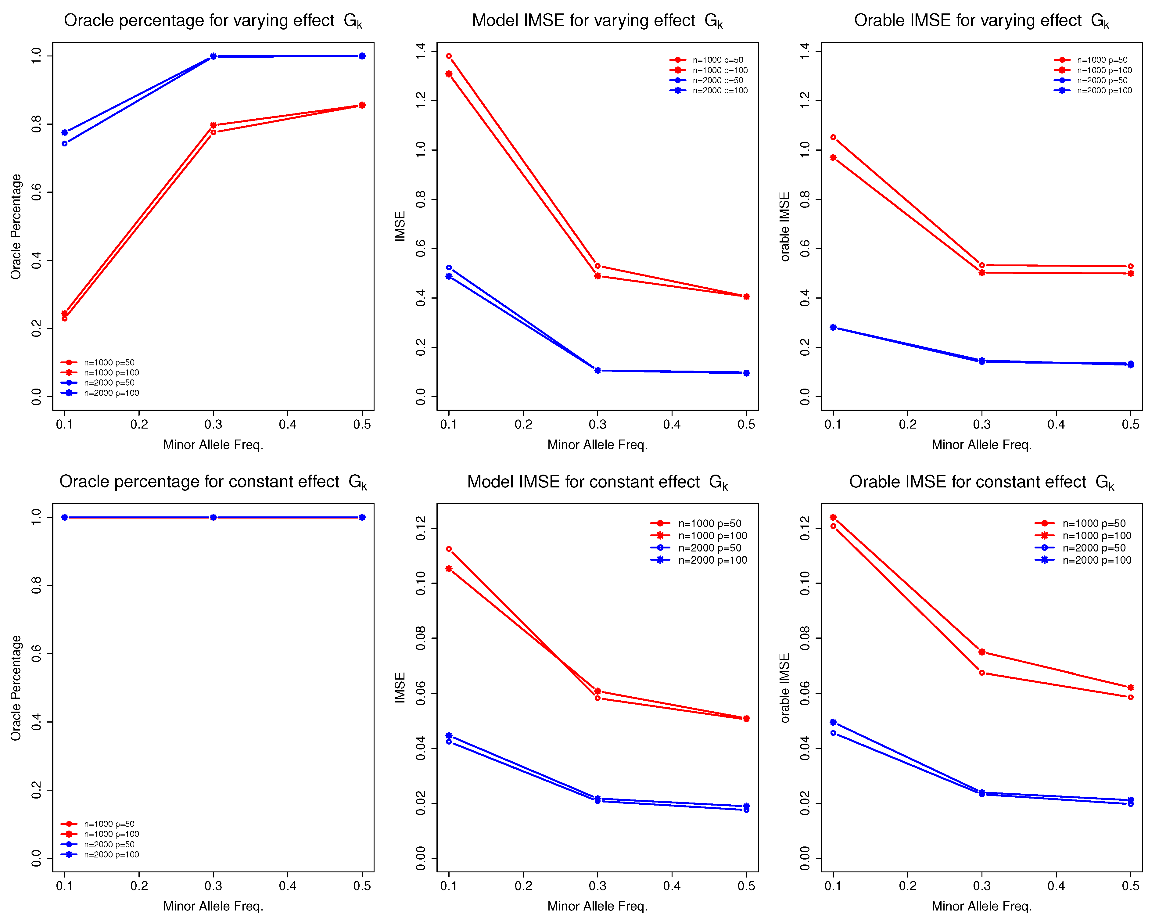
Table 4 presents the selection and estimation accuracy of the non-parametric function $m_k(·)$ for discrete G. We observed that the sample size n and MAF ($P_A$) of $G_k$ were the primary factors influencing the performance of the proposed model. To better visualize their impact, we present Figure 1.

Table 4. Selection and estimation accuracy of $m_k(·)$ for discrete predictors.

n	$\mathit{m}(·)$	$\mathit{p}=50$			$\mathit{p}=100$
		Oracle %	${\mathbf{IMSE}}_{\mathbf{Model}}$	${\mathbf{IMSE}}_{\mathbf{Oracle}}$	Oracle %	${\mathbf{IMSE}}_{\mathbf{Model}}$	${\mathbf{IMSE}}_{\mathbf{Oracle}}$
1000	$m_0(.)$	100.0	1.63$\times {10}^{-1}$	2.28$\times {10}^{-1}$	100.0	1.75$\times {10}^{-1}$	2.29$\times {10}^{-1}$
	$m_1(.)$	83.4	4.29$\times {10}^{-1}$	5.61$\times {10}^{-1}$	83.1	4.44$\times {10}^{-1}$	6.08$\times {10}^{-1}$
	$m_2(.)$	87.7	3.82$\times {10}^{-1}$	4.38$\times {10}^{-1}$	87.9	3.69$\times {10}^{-1}$	4.50$\times {10}^{-1}$
	$m_3(.)$	76.0	5.43$\times {10}^{-1}$	5.87$\times {10}^{-1}$	75.5	5.50$\times {10}^{-1}$	6.17$\times {10}^{-1}$
	$m_4(.)$	83.3	4.37$\times {10}^{-1}$	4.19$\times {10}^{-1}$	79.6	5.11$\times {10}^{-1}$	4.50$\times {10}^{-1}$
	$m_5(.)$	23.2	1.35	1.05	22.1	1.45	1.18
	$m_6(.)$	25.7	1.27	8.93$\times {10}^{-1}$	23.7	1.31	9.22$\times {10}^{-1}$
	$m_7(.)$	100.0	5.09$\times {10}^{-2}$	6.22$\times {10}^{-2}$	99.9	5.05$\times {10}^{-2}$	5.86$\times {10}^{-2}$
	$m_8(.)$	99.9	6.08$\times {10}^{-2}$	7.50$\times {10}^{-2}$	99.9	5.83$\times {10}^{-2}$	6.75$\times {10}^{-2}$
	$m_9(.)$	100.0	1.05$\times {10}^{-1}$	1.24$\times {10}^{-1}$	99.9	1.13$\times {10}^{-1}$	1.21$\times {10}^{-1}$
	Zero	99.0	2.74$\times {10}^{-3}$	0	99.2	2.15$\times {10}^{-3}$	0
2000	$m_0(.)$	100.0	7.47$\times {10}^{-2}$	8.03$\times {10}^{-2}$	100.0	7.42$\times {10}^{-2}$	8.35$\times {10}^{-2}$
	$m_1(.)$	100.0	9.46$\times {10}^{-2}$	1.38$\times {10}^{-1}$	99.9	1.02$\times {10}^{-1}$	1.49$\times {10}^{-1}$
	$m_2(.)$	100.0	9.52$\times {10}^{-2}$	1.21$\times {10}^{-1}$	99.9	9.47$\times {10}^{-2}$	1.21$\times {10}^{-1}$
	$m_3(.)$	100.0	1.07$\times {10}^{-1}$	1.55$\times {10}^{-1}$	99.8	1.08$\times {10}^{-1}$	1.50$\times {10}^{-1}$
	$m_4(.)$	99.9	1.05$\times {10}^{-1}$	1.37$\times {10}^{-1}$	99.8	1.05$\times {10}^{-1}$	1.30$\times {10}^{-1}$
	$m_5(.)$	77.5	4.84$\times {10}^{-1}$	2.99$\times {10}^{-1}$	75.1	5.15$\times {10}^{-1}$	3.08$\times {10}^{-1}$
	$m_6(.)$	77.5	4.93$\times {10}^{-1}$	2.63$\times {10}^{-1}$	73.5	5.32$\times {10}^{-1}$	2.53$\times {10}^{-1}$
	$m_7(.)$	100.0	1.89$\times {10}^{-2}$	2.11$\times {10}^{-2}$	100.0	1.75$\times {10}^{-2}$	1.97$\times {10}^{-2}$
	$m_8(.)$	100.0	2.17$\times {10}^{-2}$	2.39$\times {10}^{-2}$	100.0	2.08$\times {10}^{-2}$	2.33$\times {10}^{-2}$
	$m_9(.)$	100.0	4.47$\times {10}^{-2}$	4.95$\times {10}^{-2}$	100.0	4.24$\times {10}^{-2}$	4.56$\times {10}^{-2}$
	Zero	99.3	9.15$\times {10}^{-4}$	0	99.5	6.81$\times {10}^{-4}$	0

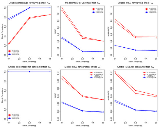
Figure 1. Selection and estimation accuracy of function $m_k(·)$ for discrete predictors under different sample sizes, data dimensions, and minor allele frequencies.

As the sample size increased (from 1000 to 2000), the model’s performance improved significantly. For instance, the oracle percentages for $m_1(·),\dots ,m_4(·)$ increased from approximately $80\%$ to nearly $100\%$, and the corresponding IMSE decreased substantially. These results align with the asymptotic theory of the proposed model. Conversely, as the MAF for ${\mathit{G}}_k$ decreased (from 0.5 to 0.1), we observed a decline in performance, reflected in both oracle percentages and model IMSE. For example, in the case where $n=1000$, the oracle percentages for $\{m_1(·),m_2(·)\}$ ($P_A=0.5$), $\{m_3(·),m_4(·)\}$ ($P_A=0.3$), and $\{m_5(·),m_6(·)\}$ ($P_A=0.1$) were approximately $85\%$, $80\%$, and $23\%$, respectively. The IMSE increased correspondingly, from 0.4 ($P_A=0.5$) to 0.5 ($P_A=0.3$) and then to 1.3 ($P_A=0.1$). This is a common phenomenon in genetic studies as smaller MAFs provide less data information to estimate the corresponding function, leading to poor estimation and selection performance.

Table 5 demonstrates the selection and estimation results for the loading parameter $\mathit{\beta }$. We observed that the sample size n was the primary factor influencing model performance. When the sample size was large ($n=2000$), the oracle percentage for non-zero loading covariates (${\beta }_1,{\beta }_2$) was $100\%$, and the oracle percentage for zero loading covariates (${\beta }_3,{\beta }_4,{\beta }_5$) was approximately $99\%$. The MSE for $\mathit{\beta }$ was in the order of ${10}^{-3}$ to ${10}^{-5}$. In contrast, when the sample size was relatively small ($n=1000$), the oracle percentage for non-zero loading covariates remained at $100\%$, but the oracle percentage for zero loading parameters decreased to around $95\%$. Comparing the cases where $p=50$ and $p=100$, we saw a slight reduction in selection accuracy for zero loading parameters when $n=1000$. This is expected, as model performance typically declines with increased model complexity. As the sample size increased to 2000, this difference in performance was not significant.

Table 5. Selection and estimation accuracy of the loading parameters $\mathit{\beta }$ for discrete predictors.

n	$\mathit{\beta }$	$\mathit{p}=50$			$\mathit{p}=100$
		Oracle %	${\mathbf{MSE}}_{\mathbf{Model}}$	${\mathbf{MSE}}_{\mathbf{Oracle}}$	Oracle %	${\mathbf{MSE}}_{\mathbf{Model}}$	${\mathbf{MSE}}_{\mathbf{Oracle}}$
1000	${\beta }_1$	100.0	6.64$\times {10}^{-4}$	7.28$\times {10}^{-4}$	100.0	5.84$\times {10}^{-4}$	5.13$\times {10}^{-4}$
	${\beta }_2$	100.0	7.37$\times {10}^{-3}$	7.32$\times {10}^{-3}$	100.0	2.76$\times {10}^{-3}$	3.27$\times {10}^{-3}$
	${\beta }_3$	95.2	3.64$\times {10}^{-4}$	0	95.2	3.73$\times {10}^{-4}$	0
	${\beta }_4$	97.0	1.21$\times {10}^{-4}$	0	96.1	4.18$\times {10}^{-4}$	0
	${\beta }_5$	96.1	2.04$\times {10}^{-4}$	0	94.7	5.46$\times {10}^{-4}$	0
2000	${\beta }_1$	100.0	2.34$\times {10}^{-4}$	2.22$\times {10}^{-4}$	100.0	2.20$\times {10}^{-4}$	2.12$\times {10}^{-4}$
	${\beta }_2$	100.0	2.31$\times {10}^{-4}$	2.20$\times {10}^{-4}$	100.0	2.30$\times {10}^{-3}$	2.37$\times {10}^{-3}$
	${\beta }_3$	98.9	5.00$\times {10}^{-5}$	0	98.9	3.24$\times {10}^{-5}$	0
	${\beta }_4$	98.7	5.44$\times {10}^{-5}$	0	98.9	4.49$\times {10}^{-5}$	0
	${\beta }_5$	98.9	4.37$\times {10}^{-5}$	0	99.0	5.07$\times {10}^{-5}$	0

Based on simulation results with both continuous and discrete G variables, we observed the following key findings about the proposed model. First, the model demonstrates robust performance with large sample sizes ($n=1000$ or 2000). Second, when $n=1000$, the false positive rate for the loading parameter $\mathit{\beta }$ was around 5%. This may reflect an inherent limitation of the LQA algorithm that cannot shrink zero parameters to exactly zero when the sample is small. Third, the model exhibits superior performance for SNP variants with larger MAFs (e.g., $P_A=0.3$ or 0.5) compared to SNP variants with smaller MAF ($P_A=0.1$). This enhanced performance likely stems from the higher amount of data information content provided by SNPs with higher MAFs. Similar phenomenon is commonly observed in other genetic association studies. Overall, the simulation results demonstrate that the method performs reasonably well under finite-sample conditions.

4. A Case Study

We demonstrated the applicability of our proposed model using a type 2 diabetes dataset containing genotypes (SNPs), environmental factors, and the phenotype (presence of type 2 diabetes). This dataset comprises two nested case–control cohort studies: the Nurses’ Health Study (NHS) and the Health Professionals Follow-Up Study (HPFS) from the Gene–Environment Association Studies Consortium (GENVEA). Detailed descriptions of these cohorts can be found in Colditz and Hankinson [13] and Rimm et al. [14]. Initially, the dataset included 3391 females (NHS) and 2599 males (HPFS).

After data cleaning, which involved removing subjects with mismatched genotypes and phenotypes, SNPs with more than $10\%$ missing data, SNPs with MAF $<0.05$, and SNPs deviating from the Hardy–Weinberg equilibrium (p-value $<0.001$), the final dataset included 5865 subjects (2494 males and 3371 females), with 2733 cases and 3132 controls, and 655,002 SNPs. The dataset also contained 12 continuous environmental factors, such as height, weight, age, and alcohol consumption. We fit a marginal logistic regression model for all 12 factors and, selected 5 environmental factors for the analysis: total physical activity ($X_1$, denoted as act), BMI ($X_2$), alcohol intake ($X_3$, denoted as alcohol), heme iron intake ($X_4$, denoted as heme), and glycemic load ($X_5$, denoted as gl). Thus, for the fitted model defined in (1), $q=5$.

Based on SNP locations, we mapped all SNPs to known genes and selected genes containing more than 30 SNPs, resulting in a total of 2178 genes. For each gene, we applied the proposed variable selection approach to identify significant SNPs and their effects. To ensure identifiability, the first element of the loading parameter $\mathit{\beta }$ was constrained to be a non-zero positive value. We fit the proposed model five times for each gene, varying the environmental factor used as the first element each time. An SNP was deemed significant if it was identified as either varying or constant across all environmental factor orders, indicating a strong signal.

In total, our model identified 13 varying-effect SNPs and 26 constant-effect SNPs. Here, we present one of the selected varying-effect SNPs as an example. Please refer to Table A1 and Table A2 in the Appendix for the complete list of selected varying- and constant-effect SNPs. Previous studies [15,16] have suggested that the gene TCF7L2 is associated with type 2 diabetes across multiple populations. Specifically, Sale et al. [15] reported a strong association between type 2 diabetes and SNPs rs7903146 and rs7901695 within this gene. Consistent with these findings, our model identified SNP rs7901695 as a constant-effect predictor, indicating no interaction with the five environmental factors (note that SNP rs7903146 was not observed in this dataset).

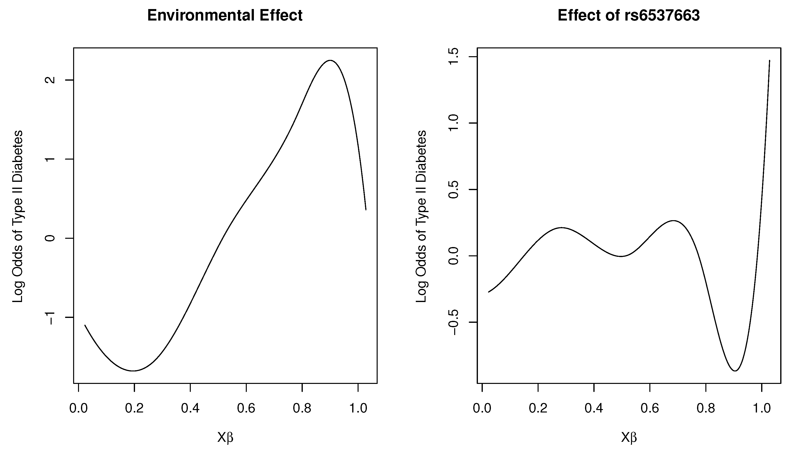
Figure 2 shows plots of the marginal total environmental effect and the interaction effect of the SNP rs6537663 in gene TCF7L2, with heme iron intake as the first loading covariate. As the index increases, we observed that the marginal effect initially decreases, then increases, and subsequently exhibits a rapid decrease as the total effect of the five environmental factors increases. For the interaction effect, it fluctuates around zero as the total effect of the five environmental variables increases, indicating that the SNP is unresponsive (or insensitive) to changes in these variables. However, as the index $\mathit{X}\mathit{\beta }$ continues to increase, the SNP reacts to environmental changes, with a dramatic increase in risk for type 2 diabetes beyond a certain threshold. This estimated effect suggests that the genetic sensitivity of the SNP to the total effect of the five environmental variables follows a threshold model. This finding has practical implications: most individuals tolerate daily environmental changes, including dietary variations, without adverse effects. However, when such changes exceed a certain limit, the risk of disease may increase.

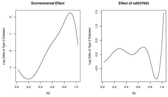
Figure 2. Plot of varying effects on a log-odds scale for SNP rs6537663 in Gene TCF7L2.

Table 6 presents the selection and estimation results of the loading parameters $\mathit{\beta }$, with heme iron intake as the first loading covariate. The model selects all loading parameters except for alcohol consumption (alcohol). Notably, we observed that body mass index (BMI) has the largest effect, which aligns with practical knowledge, as BMI is positively associated with type 2 diabetes and is a well-established risk factor for the disease. Notably, the sign of the loading parameters aligns with known associations in the literature. For example, Hu et al. [17] reported that higher physical activity is linked to a lower risk of type 2 diabetes, while Field et al. [18] demonstrated that high BMI increases the risk of type 2 diabetes. Additionally, Rajpathak et al. [19] found that high heme iron intake is associated with an increased risk of type 2 diabetes, and Salmerón et al. [20] showed that a high glycemic load is linked to a higher risk of type 2 diabetes. The signs of the estimated loading coefficients are consistent with these established findings.

Table 6. Estimation and selection result for $\mathit{\beta }$.

Act	BMI	Alcohol	Heme	gl
−0.1832	0.9544	0	0.2157	0.0947

5. Discussion

G × E interactions have been extensively studied in the literature, leading to the development of numerous statistical models. In this paper, we propose a three-step iterative variable selection approach for the generalized single-index varying-coefficients model (gSIVCM) with a binary response. Our goal is to identify varying, constant, and zero-effect genes, as well as to select non-zero environmental factors that interact with varying-effect genes. Biologically, our approach is attractive as it provides a novel perspective on G × E interactions. The flexibility of our model allows for the detection of non-linear interactions, making it particularly suitable when gene effects are non-linearly influenced by simultaneous exposure to multiple environmental factors. Statistically, gSIVCM reduces the dimensionality of the model by treating multiple indices X as a single index, which significantly alleviates the curse of dimensionality when multiple environmental factors interact with gene effects.

For the theorem presented in this work, we note that while the regularity conditions provide theoretical guarantees for the method’s performance, their applicability in real-world settings may be uncertain. Directly checking these conditions is typically infeasible due to the complexity and high-dimensional nature of real-world data. Despite these challenges, we emphasize that the method has shown strong empirical performance in various settings, including simulations and case studies. This suggests that the assumptions, while idealized, may approximate practical scenarios sufficiently well in many cases. We propose that future research could focus on developing diagnostic tools to assess whether the underlying assumptions are reasonable for a given dataset or on extending the method to relax these conditions.

Our work builds upon the framework introduced by Guan et al. [4] with a three-step variable selection approach for SIVCM with continuous responses. We extended our previous work to binary responses, broadening its applicability to a wider range of biological studies. For continuous responses, researchers are often interested in specific quantiles of the response, such as birth weight, rather than the mean. It is a natural progression to extend our variable selection approach to quantile regression settings, which we plan to explore in future studies. In addition, the methodology proposed in this paper can be readily generalized to include other discrete response variables with appropriate use of link functions. Another interesting direction for future research would be to adapt the selection procedure developed in the multivariate framework to the functional data framework. This idea has been explored in a general context by Aneiros et al. [21] and more specifically in the context of partial single-index modeling by Novo et al. [22]. Additionally, a broader survey of applications for this concept can be found in Aneiros et al. [23]. While this paper focuses on the multivariate framework, exploring these connections in the functional data setting could open new avenues for methodological advancements.

While the proposed method demonstrates strong empirical performance, several limitations warrant discussion. First, the computational cost of fitting high-dimensional datasets can be substantial, particularly when dealing with large-scale genomic or pathway-based analyses. Second, the success of the method depends on the validity of the regularity conditions, which may not always hold in noisy or sparsely sampled data. For example, dependencies among predictors or unmeasured confounding factors could affect the accuracy of variable selection. Finally, the interpretability of selected indices and varying coefficients may require domain expertise, limiting accessibility for practitioners without a statistical background. To further validate the robustness and utility of the method, additional testing on datasets with diverse characteristics, such as varying levels of noise, sample sizes, or population structures, would be beneficial. These studies would help establish the method’s adaptability to different study designs and its potential limitations in specific scenarios.

Among the listed genes in Table A1 in the appendix, ABCA1 and NTRK2 show strong evidence of association with type 2 diabetes (T2D), with ABCA1 influencing lipid metabolism and insulin secretion [24,25] and NTRK2 regulating energy balance and glucose metabolism via BDNF signaling [26]. Genes such as GALNT2, PTK2B, and RBM15-AS1 are linked to metabolic pathways or inflammation, indirectly influencing T2D risk [27,28,29]. Other genes, including LARS2, UNC5C, and SCAI, have limited or emerging evidence, often tied to mitochondrial dysfunction, apoptosis, or cellular stress, highlighting the need for further investigation into their roles in T2D pathogenesis [30,31,32]. For genes listed in Table A2, TCF7L2 stands out as a well-established genetic risk factor for T2D. Variants in TCF7L2 are strongly associated with impaired insulin secretion and glucose metabolism, contributing significantly to T2D susceptibility [33]. Another important gene is GALNT2, which has been implicated in lipid and glucose metabolism; polymorphisms in this gene are linked to alterations in glycemic traits and may indirectly influence T2D risk [27]. For the other genes, though no strong evidence directly linking them to T2D has been identified in the current literature, they may still play roles in metabolic or cellular pathways relevant to diabetes pathophysiology, warranting further investigation. It is worth noting that the findings generated by our algorithm are intended to serve as a statistical foundation for further exploration by experts in the field.

In this work, we demonstrated the model’s applicability through a gene-based analysis. Our method can also be extended to pathway-based analysis. In the human genome, pathways typically include a diverse array of genes, with each gene containing hundreds to thousands of SNPs. A pathway-based SNP-level analysis can be conducted by modeling SNPs within a pathway as genetic variables. Alternatively, a pathway-based gene-level analysis can be performed by summarizing the genomic information of each gene into a few principal components (PCs) using principal component analysis (PCA) [34] or sparse principal component analysis (sPCA) [35]. The proposed method can then be applied to select significant PCs within a pathway, facilitating the identification of key interactions between genes and environmental mixtures. By accounting for the genomic structure, this pathway-based approach has the potential to yield more interpretable and biologically meaningful results. Moreover, the ability to extend gSIVCM to quantile regression and functional data broadens its applicability significantly. For instance, quantile regression could allow researchers to explore G × E interactions at various points in the response distribution, such as studying low birth weight or extreme phenotypes in epidemiological studies. Similarly, applying the method to functional data could be transformative in fields like neuroscience or metabolomics, where variables are often measured continuously over time or space.

Appendix A.1. Computational Algorithm

Step 1 and Step 2 follow directly from the group coordinate descent algorithm shown in the main text, and we omit the details here.

Step 3:

$$\widehat{\mathit{\beta }}=\underset{{\left|\right|\mathit{\beta }\left|\right|}_2=1}{max}{M}_3\left(\mathit{\beta }\right|{\lambda }_3,{\widehat{\mathit{\gamma }}}^{\left(2\right)})=\underset{{\left|\right|\mathit{\beta }\left|\right|}_2=1}{max}\left(l({\widehat{\mathit{\gamma }}}^{\left(2\right)},\mathit{\beta })-n\sum _{d=2}^q{p}_{{\lambda }_3}\left(\right|{\beta }_d\left|\right)\right).$$

Since this is a penalized likelihood problem, we adopt the local quadratic approximation (LQA) approach proposed by Fan and Li [5]. Let $\tilde{\mathit{\beta }}$ denote the most recent value of $\mathit{\beta }$. By applying Taylor expansion at $\tilde{\mathit{\beta }}$, we obtain the following:

$$l({\widehat{\mathit{\gamma }}}^{\left(2\right)},\mathit{\beta })\approx l({\widehat{\mathit{\gamma }}}^{\left(2\right)},\tilde{\mathit{\beta }})+▽l{({\widehat{\mathit{\gamma }}}^{\left(2\right)},\tilde{\mathit{\beta }})}^T(\mathit{\beta }-\tilde{\mathit{\beta }})+{\displaystyle \frac{1}{2}}{(\mathit{\beta }-\tilde{\mathit{\beta }})}^T{▽}^{2}l({\widehat{\mathit{\gamma }}}^{\left(2\right)},\tilde{\mathit{\beta }})(\mathit{\beta }-\tilde{\mathit{\beta }})$$

where

$$▽l({\widehat{\mathit{\gamma }}}^{\left(2\right)},\tilde{\mathit{\beta }})={({\displaystyle \frac{\partial l({\widehat{\mathit{\gamma }}}^{\left(2\right)},\mathit{\beta })}{\partial {\beta }_1}},\dots ,{\displaystyle \frac{\partial l({\widehat{\mathit{\gamma }}}^{\left(2\right)},\mathit{\beta })}{\partial {\beta }_q}})}^T{|}_{\mathit{\beta }=\tilde{\mathit{\beta }}}\mathrm{is}\mathrm{the}\mathrm{gradient}$$

$${▽}^{2}l({\widehat{\mathit{\gamma }}}^{\left(2\right)},\tilde{\mathit{\beta }})={\left[{\displaystyle \frac{{\partial }^{2}l({\widehat{\mathit{\gamma }}}^{\left(2\right)},\mathit{\beta })}{\partial {\beta }_j\partial {\beta }_l}}\right]}_{1\le j,l\le q}{|}_{\mathit{\beta }=\tilde{\mathit{\beta }}}\mathrm{is}\mathrm{the}\mathrm{hessian}\mathrm{matrix},$$

and

$${\displaystyle \frac{\partial l({\widehat{\mathit{\gamma }}}^{\left(2\right)},\mathit{\beta })}{\partial {\beta }_j}}={(\mathit{Y}-{\displaystyle \frac{1}{1+e^{-{\mathit{\mu }}^{B^{\left(3\right)}}}}})}^T{\displaystyle \frac{\partial {\mathit{\mu }}^{B^{\left(3\right)}}}{\partial {\beta }_j}}$$

$${\displaystyle \frac{{\partial }^{2}l({\widehat{\mathit{\gamma }}}^{\left(2\right)},\mathit{\beta })}{\partial {\beta }_j\partial {\beta }_l}}={(\mathit{Y}-{\displaystyle \frac{1}{1+e^{-{\mathit{\mu }}^{B^{\left(3\right)}}}}})}^T{\displaystyle \frac{\partial {\mathit{\mu }}^{B^{\left(3\right)}}}{\partial {\beta }_j\partial {\beta }_l}}-{\left({\displaystyle \frac{e^{-{\mathit{\mu }}^{B^{\left(3\right)}}}}{{(1+e^{-{\mathit{\mu }}^{B^{\left(3\right)}}})}^2}}\right)}^T{\displaystyle \frac{\partial {\mathit{\mu }}^{B^{\left(3\right)}}}{{\partial }_{{\beta }_j}}}·{\displaystyle \frac{\partial {\mathit{\mu }}^{B^{\left(3\right)}}}{{\partial }_{{\beta }_l}}},$$

and

$${\mathit{\mu }}^{B^{\left(3\right)}}=\sum _{k=0}^p[{\widehat{\gamma }}_{k1}^{\left(2\right)}+\overline{\mathit{B}}\left(\mathit{X}\mathit{\beta }\right){\widehat{\mathit{\gamma }}}_{k\ast }^{\left(2\right)}]·{\mathit{G}}_k,$$

$${\displaystyle \frac{\partial {\mathit{\mu }}^{B^{\left(3\right)}}}{\partial {\beta }_j}}=\sum _{k=0}^p\left({\overline{\mathit{B}}}^{\prime }\left(\mathit{X}\mathit{\beta }\right){\widehat{\mathit{\gamma }}}_{k\ast }^{\left(2\right)}·{\mathit{X}}_j·{\mathit{G}}_k\right),$$

$${\displaystyle \frac{\partial {\mathit{\mu }}^{B^{\left(3\right)}}}{\partial {\beta }_j\partial {\beta }_l}}=\sum _{k=0}^p\left({\overline{\mathit{B}}}^{″}\left(\mathit{X}\mathit{\beta }\right){\widehat{\mathit{\gamma }}}_{k\ast }^{\left(2\right)}·{\mathit{X}}_j·{\mathit{X}}_l·{\mathit{G}}_k\right).$$

Let

$${\mathbf{\Sigma }}_{{\lambda }_3}\left(\tilde{\mathit{\beta }}\right)=diag(0,{\displaystyle \frac{p_{{\lambda }_3}^{\prime }\left(\widehat{{\beta }_2}\right)}{|\widehat{{\beta }_2}|}},\dots ,{\displaystyle \frac{p_{{\lambda }_3}^{\prime }\left(\widehat{{\beta }_q}\right)}{|\widehat{{\beta }_q}|}}).$$

We update $\mathit{\beta }$ as follows:

$${\mathit{\beta }}^{\ast }=\tilde{\mathit{\beta }}-{\left[{▽}^{2}l({\widehat{\mathit{\gamma }}}^{\left(2\right)},\tilde{\mathit{\beta }})+n{\mathbf{\Sigma }}_{{\lambda }_3}\left(\tilde{\mathit{\beta }}\right)\right]}^{-1}\left[▽l({\widehat{\mathit{\gamma }}}^{\left(2\right)},\tilde{\mathit{\beta }})+n{\mathbf{\Sigma }}_{{\lambda }_3}\left(\tilde{\mathit{\beta }}\right)\tilde{\mathit{\beta }}\right].$$

The updated value of $\mathit{\beta }$ is then obtained through standardization:

$${\mathit{\beta }}^{\mathrm{updated}}=\mathrm{sign}\left({\beta }_1^{\ast }\right){\displaystyle \frac{{\mathit{\beta }}^{\ast }}{\left|\right|{\mathit{\beta }}^{\ast }{\left|\right|}_2}}.$$

Finally, we iterate this process until convergence.

Appendix A.2. Proofs of Theorems

Appendix A.2.1. Notations

Let the space of Lipschitz continuous functions for any fixed constant c be denoted as $Lip([a,b],c)=\{f:|f\left(x_1\right)-f\left(x_2\right)|\le c|x_1-x_2|,\forall x_1,x_2\in [a,b]\}$. Define $C^{\left(p\right)}[a,b]=\{f:f^{\left(p\right)}\in C[a,b]\}$ as the space of p-th order smooth functions.

Appendix A.2.2. Some Regularity Conditions

(A1)

The density function $f_{U\left(\mathit{\beta }\right)}(.)$ of the random variable $U\left(\mathit{\beta }\right)=\mathit{X}\mathit{\beta }$ is bounded away from 0 on $\mathbf{\Omega }=\{\mathit{X}\mathit{\beta },\mathit{X}\in \mathcal{X}\}$, where $\mathcal{X}$ is the compact support of X. There exists a constant $c_1$ such that $f_{U\left(\mathit{\beta }\right)}(.)\in Lip([a,b],c_1)$.

(A2)

For $k=0,1,\dots ,p$, the non-parametric function $m_k(.)\in C^{\left(r\right)}$ with $r\ge 2$.

(A3)

$E\left(\right|\left|\mathit{G}\right|{|}^6)<\infty$.

(A4)

The matrix $\mathit{M}\left(u\right)=E\left(\mathit{G}{\mathit{G}}^T\right|\mathit{X}\mathit{\beta }=u)$ is positive definite, and each element of $\mathit{M}\left(u\right)\in Lip([a,b],c_4)$.

(A5)

Define

$$b_n=\underset{k,l}{max}\{p_{{\lambda }_1}^{″}\left(\right||{\mathit{\gamma }}_{k\ast }^0{\left|\right|}_2),p_{{\lambda }_2}^{″}\left(\right|{\mathit{\gamma }}_{k1}^0\left|\right),p_{{\lambda }_3}^{″}\left(\right|{\beta }_d^0\left|\right):{\mathit{\gamma }}_{k\ast }^0\ne 0,{\mathit{\gamma }}_{k1}^0\ne 0,{\beta }_l^0\ne 0\}.$$

For $k=1,\dots ,p$ and $d=2,\dots ,q$, it holds that $b_n\to 0$ as $n\to \infty$.

(A6)

$$\underset{n\to \infty }{lim\; inf}\underset{\left|\right|{\mathit{\gamma }}_{k\ast }{\left|\right|}_2\to 0^{+}}{lim\; inf}{\displaystyle \frac{1}{{\lambda }_1}}|p_{{\lambda }_1}^{\prime }\left(\right||{\mathit{\gamma }}_{k\ast }{\left|\right|}_2\left)\right|>0\mathrm{for}k=v+1,\dots ,p,$$

$$\underset{n\to \infty }{lim\; inf}\underset{|{\mathit{\gamma }}_{k1}|\to 0^{+}}{lim\; inf}{\displaystyle \frac{1}{{\lambda }_2}}|p_{{\lambda }_2}^{\prime }\left(\right|{\mathit{\gamma }}_{k1}\left|\right)|>0\mathrm{for}k=c+1,\dots ,p,$$

$$\underset{n\to \infty }{lim\; inf}\underset{|{\beta }_d|\to 0^{+}}{lim\; inf}{\displaystyle \frac{1}{{\lambda }_3}}|p_{{\lambda }_3}^{\prime }\left(\right|{\beta }_d\left|\right)|>0\mathrm{for}d=s+1,\dots ,q.$$

(A7)

Let $c_1,\dots ,c_K$ be internal points of $[a,b]$, where $a=inf\{u:u\in \mathbf{\Omega }\}$ and $b=sup\{u:u\in \mathbf{\Omega }\}$. Define $c_0=a$, $c_{K+1}=b$, $h_i=c_i-c_{i-1}$. There exists a constant $C_7$ such that $max\left\{h_i\right\}/min\left\{h_i\right\}<C_7$, and $max\left\{h_{i+1}{h}_i\right\}=o\left(K^{-1}\right)$.

Appendix A.2.3. Proof of Theorem 1

Let $\mathit{\varphi }={({\beta }_2,\dots ,{\beta }_q)}^T$, and we have $\mathit{\beta }={(\sqrt{1-{\left|\right|\mathit{\varphi }\left|\right|}_2^2},{\mathit{\varphi }}^T)}^T$, hence the restriction $\left|\right|\mathit{\beta }\left|\right|=1$ and ${\beta }_1>0$ is equivalent to ${\left|\right|\mathit{\varphi }\left|\right|}_2<1$. To show the consistency of $\widehat{\mathit{\beta }}$, it is enough to show the consistency of $\widehat{\mathit{\varphi }}$.

Define ${\alpha }_n=n^{-r/(2r+1)}+a_n$, $\mathit{\gamma }={\mathit{\gamma }}^0+{\alpha }_n{\mathit{\tau }}_1$, $\mathit{\varphi }={\mathit{\varphi }}^0+{\alpha }_n{\mathit{\tau }}_2$, and $\mathit{\tau }=({\mathit{\tau }}_1,{\mathit{\tau }}_2)$, where ${\mathit{\tau }}_1=({\tau }_{01},{\mathit{\tau }}_{0\ast },\dots ,{\tau }_{p1},{\mathit{\tau }}_{p\ast })$ and $\{{\tau }_{k1},{\mathit{\tau }}_{k\ast }\}$ correspond to the B-spline coefficients ${\gamma }_{k1},{\mathit{\gamma }}_{k\ast }$. Similarly, ${\mathit{\tau }}_2=({\tau }_1^{\varphi },\dots ,{\tau }_{q-1}^{\varphi })$, where ${\tau }_l^{\varphi }$ corresponds to ${\varphi }_l$.

To establish the consistency of $\widehat{\mathit{\gamma }}$ and $\widehat{\mathit{\varphi }}$, we need to show that $\forall ϵ>0$, ∃ a sufficiently large C, such that

$$P\left(\underset{\left|\right|\mathit{\tau }\left|\right|=C}{sup}\left\{M(\mathit{\gamma },\mathit{\varphi })\right\}<M({\mathit{\gamma }}^0,{\mathit{\varphi }}^0)\right)\ge 1-ϵ,$$

(A1)

where

$$M(\mathit{\gamma },\mathit{\varphi })=l(\mathit{\gamma },\mathit{\varphi })-n\sum _{k=1}^p{p}_{{\lambda }_1}\left(\right||{\mathit{\gamma }}_{k\ast }{\left|\right|}_2)-n\sum _{k=1}^p{p}_{{\lambda }_2}\left(\right|{\gamma }_{k1}\left|\right)I\left(\right||{\mathit{\gamma }}_{k\ast }{\left|\right|}_2=0)-n\sum _{l=1}^{q-1}{p}_{{\lambda }_3}\left(\right|{\varphi }_l\left|\right),$$

and $l(\mathit{\gamma },\mathit{\varphi })$ is the log-likelihood function defined above. If (A1) holds, it implies that with probability at least $1-ϵ$, there exists a local maximum within the ball $\{({\mathit{\gamma }}^0,{\mathit{\varphi }}^0)+{\alpha }_n\mathit{\tau }:|\left|\mathit{\tau }\right||\le C\}$. Hence, there exists a local maximizer such that $\left|\right|(\widehat{\mathit{\gamma }},\widehat{\mathit{\varphi }})-({\mathit{\gamma }}^0,{\mathit{\varphi }}^0)\left|\right|=O_p\left({\alpha }_n\right)$.

Define

$$\begin{array}{ccc}\hfill D_n\left(\mathit{\tau }\right)& ={\displaystyle \frac{1}{K}}\{M(\mathit{\gamma },\mathit{\varphi })-M({\mathit{\gamma }}^0,{\mathit{\varphi }}^0)\}={\displaystyle \frac{1}{K}}\{M({\mathit{\gamma }}^0+{\alpha }_n{\mathit{\tau }}_1,{\mathit{\varphi }}^0+{\alpha }_n{\mathit{\tau }}_2)-M({\mathit{\gamma }}^0,{\mathit{\varphi }}^0)\}\hfill & \\ & ={\displaystyle \frac{1}{K}}\{\left[l({\mathit{\gamma }}^0+{\alpha }_n{\mathit{\tau }}_1,{\mathit{\varphi }}^0+{\alpha }_n{\mathit{\tau }}_2)-l({\mathit{\gamma }}^0,{\mathit{\varphi }}^0)\right]-n\sum _{k=1}^p\left[p_{{\lambda }_1}\left(\right||{\mathit{\gamma }}_{k\ast }^0+{\alpha }_n{\mathit{\tau }}_{k\ast }{\left|\right|}_2)-p_{{\lambda }_1}\left(\right||{\mathit{\gamma }}_{k\ast }^0{\left|\right|}_2)\right]\hfill & \\ & -n\sum _{k=1}^p\left[p_{{\lambda }_2}\left(\right|{\gamma }_{k1}^0+{\alpha }_n{\tau }_{k1}\left|\right)I\left(\right||{\mathit{\gamma }}_{k\ast }^0+{\alpha }_n{\tau }_{k\ast }{\left|\right|}_2=0)-p_{{\lambda }_2}\left(\right|{\gamma }_{k1}^0\left|\right)I\left(\right||{\mathit{\gamma }}_{k\ast }^0{\left|\right|}_2=0)\right]\hfill & \\ & -n\sum _{j=1}^{q-1}\left[p_{{\lambda }_3}\left(\right|{\varphi }_j^0+{\alpha }_n{\tau }_j^{\varphi }\left|\right)-p_{{\lambda }_3}\left(\right|{\varphi }_j^0\left|\right)\right]\}.\hfill \end{array}$$

Since $p_{{\lambda }_1}\left(\right||{\mathit{\gamma }}_{k\ast }^0{\left|\right|}_2)=0$ for $k=v+1,\dots ,p$, $p_{{\lambda }_3}\left(\right|{\varphi }_j^0\left|\right)=0$ for $j=s+1,\dots ,q-1$, and $I\left(\right|\left|{\mathit{\gamma }}_{k\ast }^0\right|{|}_2=0)=0$ for $k=1,\dots ,v$, we have the following:

$$\begin{array}{ccc}\hfill D_n\left(\mathit{\tau }\right)& \le {\displaystyle \frac{1}{K}}\{l({\mathit{\gamma }}^0+{\alpha }_n{\mathit{\tau }}_1,{\mathit{\varphi }}^0+{\alpha }_n{\mathit{\tau }}_2)-l({\mathit{\gamma }}^0,{\mathit{\varphi }}^0)\hfill & \\ & -n\sum _{k=1}^v[p_{{\lambda }_1}\left(\right||{\mathit{\gamma }}_{k\ast }^0+{\alpha }_n{\mathit{\tau }}_{k\ast }{\left|\right|}_2)-p_{{\lambda }_1}\left(\right||{\mathit{\gamma }}_{k\ast }^0{\left|\right|}_2\left)\right]\hfill & \\ & -n\sum _{k=v+1}^p\left[p_{{\lambda }_2}\left(\right|{\gamma }_{k1}^0+{\alpha }_n{\tau }_{k1}\left|\right)-p_{{\lambda }_2}\left(\right|{\gamma }_{k1}^0\left|\right)\right]\hfill & \\ & -n\sum _{j=1}^{s-1}[p_{{\lambda }_3}\left(\right|{\varphi }_j^0+{\alpha }_n{\tau }_j^{\varphi }\left|\right)-p_{{\lambda }_3}\left(\right|{\varphi }_j^0\left|\right)\left]\right\}.\hfill \end{array}$$

Applying Taylor expansion at $({\mathit{\gamma }}^0,{\mathit{\varphi }}^0)$ and simplifying the bounds for $D_n\left(\mathit{\tau }\right)$, we derive that

$$\left|\right|(\widehat{\mathit{\gamma }},\widehat{\mathit{\varphi }})-({\mathit{\gamma }}^0,{\mathit{\varphi }}^0)\left|\right|=O_p\left({\alpha }_n\right).$$

where $\mathit{I}({\mathit{\gamma }}^0,{\mathit{\varphi }}^0)$ is the Fisher information matrix. By standard arguments of likelihood theory, $S_1$ is of the order $O_p(1+n^{r/(2r+1)}{\alpha }_n)\left|\right|\mathit{\tau }\left|\right|$, $S_2$ is of the order $O_p(1+2n^{r/(2r+1)}{\alpha }_n){\left|\right|\mathit{\tau }\left|\right|}^2$, and for sufficiently large C, $S_2$ dominates $S_1$ uniformly in $\left|\right|\mathit{\tau }\left|\right|=C$. Furthermore, we have

$$\begin{array}{ccc}\hfill S_3& \le {\displaystyle \frac{n}{K}}{\alpha }_n{a}_n\sum _{k=1}^v{\displaystyle \frac{{\mathit{\gamma }}_{k\ast }^0}{\left|\right|{\mathit{\gamma }}_{k\ast }^0{\left|\right|}_2}}{\mathit{\tau }}_{k\ast }^T+{\displaystyle \frac{n}{K}}{\alpha }_n^2\underset{k}{max}\{p_{{\lambda }_1}^{″}\left(\right||{\mathit{\gamma }}_{k\ast }^0{\left|\right|}_2\left)\right\}\sum _{k=1}^v{\mathit{\tau }}_{k\ast }{\mathit{\tau }}_{k\ast }^T\hfill & \\ & \le {\displaystyle \frac{n}{K}}{\alpha }_n^2\sqrt{v}\left|\right|\mathit{\tau }\left|\right|+{\displaystyle \frac{n}{K}}{\alpha }_n^2{\left|\right|\mathit{\tau }\left|\right|}^2\underset{k}{max}\{p_{{\lambda }_1}^{″}\left(\right||{\mathit{\gamma }}_{k\ast }^0{\left|\right|}_2\left)\right\}.\hfill \end{array}$$

Since ${max}_k\{p_{{\lambda }_1}^{″}\left(\right||{\mathit{\gamma }}_{k\ast }^0{\left|\right|}_2\left)\right\}\to 0$, we conclude that $S_3$ is dominated by $S_2$.

For $S_4$ and $S_5$, we have the following:

$$\begin{array}{ccc}\hfill S_4& \le & {\alpha }_n{a}_n{\displaystyle \frac{n}{K}}\sum _{k=v+1}^p{\tau }_{k1}+{\displaystyle \frac{n}{K}}{\alpha }_n^2\underset{k}{max}\{p_{{\lambda }_2}^{″}\left(\right|{\gamma }_{k1}^0\left|\right)\}\sum _{k=v+1}^p{\left({\tau }_{k1}\right)}^2\hfill \\ & \le & {\displaystyle \frac{n}{K}}{\alpha }_n^2\left|\right|\mathit{\tau }\left|\right|+{\displaystyle \frac{n}{K}}{\alpha }_n^2{\left|\right|\mathit{\tau }\left|\right|}^2\underset{k}{max}\{p_{{\lambda }_2}^{″}\left(\right|{\gamma }_{k1}^0\left|\right)\},\hfill \end{array}$$

and

$$\begin{array}{ccc}\hfill S_5& \le & {\alpha }_n{a}_n{\displaystyle \frac{n}{K}}\sum _{l=1}^{s-1}{\tau }_l^{\varphi }+{\displaystyle \frac{n}{K}}{\alpha }_n^2\underset{l}{max}\{p_{{\lambda }_3}^{″}\left(\right|{\varphi }_l^0\left|\right)\}\sum _{l=1}^{s-1}{\left({\tau }_l^{\varphi }\right)}^2\hfill \\ & \le & {\displaystyle \frac{n}{K}}{\alpha }_n^2\left|\right|\mathit{\tau }\left|\right|+{\displaystyle \frac{n}{K}}{\alpha }_n^2{\left|\right|\mathit{\tau }\left|\right|}^2\underset{l}{max}\{p_{{\lambda }_3}^{″}\left(\right|{\varphi }_l^0\left|\right)\}.\hfill \end{array}$$

Similarly, $S_4$ and $S_5$ are dominated by $S_2$. Thus, by choosing a sufficiently large C, we obtain $\left|\right|(\widehat{\mathit{\gamma }},\widehat{\mathit{\varphi }})-({\mathit{\gamma }}^0,{\mathit{\varphi }}^0)\left|\right|=O_p\left({\alpha }_n\right)$. Therefore, the consistency of the penalized least squares estimator $(\widehat{\mathit{\gamma }},\widehat{\mathit{\varphi }})$ is proven.

Appendix A.2.4. Proof of Theorem 2

For (i), for ease of notation, let $\mathit{\varphi }=({\mathit{\varphi }}^{nz},{\mathit{\varphi }}^z)$, where ${\mathit{\varphi }}^{nz}=({\varphi }_1,\dots ,{\varphi }_{s-1})$ and ${\mathit{\varphi }}^z=({\varphi }_s,\dots ,{\varphi }_{q-1})$. Since ${\lambda }_{\max }\to 0$, it follows that $a_n=0$ for sufficiently large n. By Theorem 1, it suffices to show that for ${\mathit{\varphi }}^{nz}$,

$$\left|\right|{\varphi }_l-{\varphi }_l^0{\left|\right|}_2=O_p\left(n^{-r/(2r+1)}\right),l=1,\dots ,s-1,$$

and for ${\mathit{\varphi }}^z$, there exists a small constant $ϵ=C{n}^{-r/(2r+1)}$ such that as $n\to \infty$, with probability approaching 1, for $l=s,\dots ,q-1$, we have the following:

$${\displaystyle \frac{\partial M(\mathit{\gamma },\mathit{\varphi })}{\partial {\varphi }_l}}<0\mathrm{when}0<{\varphi }_l<ϵ,\mathrm{and}{\displaystyle \frac{\partial M(\mathit{\gamma },\mathit{\varphi })}{\partial {\varphi }_l}}>0\mathrm{when}-ϵ<{\varphi }_l<0.$$

We start with

$${\displaystyle \frac{\partial M(\mathit{\gamma },\mathit{\varphi })}{\partial {\varphi }_l}}={\displaystyle \frac{\partial l(\mathit{\gamma },\mathit{\varphi })}{\partial {\varphi }_l}}-n{p}_{{\lambda }_3}^{\prime }\left(\right|{\varphi }_l\left|\right)sign\left({\varphi }_l\right).$$

Then, expanding $\partial l(\mathit{\gamma },\mathit{\varphi })/\partial {\varphi }_l$ at ${\mathit{\varphi }}^0$ using a Taylor expansion, we obtain the following:

$$\begin{array}{ccc}\hfill {\displaystyle \frac{\partial M(\mathit{\gamma },\mathit{\varphi })}{\partial {\varphi }_l}}& ={\displaystyle \frac{\partial l(\mathit{\gamma },{\mathit{\varphi }}^0)}{\partial {\varphi }_l}}+\sum _{k=1}^{q-1}{\displaystyle \frac{{\partial }^{2}l(\mathit{\gamma },{\mathit{\varphi }}^0)}{\partial {\varphi }_l\partial {\varphi }_k}}({\varphi }_k-{\varphi }_k^0)\hfill & \\ & +\sum _{k=1}^{q-1}\sum _{j=1}^{q-1}{\displaystyle \frac{{\partial }^{3}l(\mathit{\gamma },{\mathit{\varphi }}^{\ast })}{\partial {\varphi }_l\partial {\varphi }_k\partial {\varphi }_j}}({\varphi }_k-{\varphi }_k^0)({\varphi }_j-{\varphi }_j^0)-n{p}_{{\lambda }_3}^{\prime }\left(\right|{\varphi }_l\left|\right)sign\left({\varphi }_l\right),\hfill \end{array}$$

where ${\mathit{\varphi }}^{\ast }$ lies between ${\mathit{\varphi }}^0$ and $\mathit{\varphi }$. After simplification, we derive the following:

$${\displaystyle \frac{\partial M(\mathit{\gamma },\mathit{\varphi })}{\partial {\varphi }_l}}=n{\lambda }_3\left\{-{\displaystyle \frac{1}{{\lambda }_3}}{p}_{{\lambda }_3}^{\prime }\left(\right|{\varphi }_l\left|\right)sign\left({\varphi }_l\right)+O_p\left({\displaystyle \frac{1}{{\lambda }_3}}{n}^{-r/(2r+1)}\right)\right\}.$$

Since ${lim}_{n\to \infty }{lim\; inf}_{{\varphi }_l\to 0}{\displaystyle \frac{1}{{\lambda }_3}}{p}_{{\lambda }_3}^{\prime }\left(\right|{\varphi }_l\left|\right)>0$ and ${\displaystyle \frac{1}{{\lambda }_3}}{n}^{-r/(2r+1)}\to 0$, the sign of $\partial M(\mathit{\gamma },\mathit{\varphi })/\partial {\varphi }_l$ is completely determined by $sign\left({\varphi }_l\right)$. Thus, we conclude ${\widehat{\beta }}_j=0$ for $j=s+1,\dots ,q-1$.

For (ii) & (iii), by applying similar arguments as in part (i), it follows that with probability approaching 1, ${\widehat{\mathit{\gamma }}}_{k\ast }=0$ for $k=v+1,\dots ,p$ and ${\widehat{\gamma }}_{k1}=0$ for $k=c+1,\dots ,p$. Using ${sup}_u\mathit{B}\left(u\right)=O\left(1\right)$ and the fact that ${\widehat{m}}_k\left(u\right)={\widehat{\gamma }}_{k0}+\overline{\mathit{B}}\left(\mathit{X}\widehat{\mathit{\beta }}\right){\widehat{\mathit{\gamma }}}_{k\ast }$, we have the following:

$${\widehat{m}}_k\left(u\right)=c_k,k=v+1,\dots ,c,$$

where $c_k$ is a constant, and

$${\widehat{m}}_k\left(u\right)=0,k=c+1,\dots ,p.$$

This completes the proof.

Appendix A.3. Additional Real Data Analysis Results

Table A1 lists all the varying-effect SNPs selected, along with the gene IDs to which they were mapped. Similarly, Table A2 provides a summary of all the constant-effect SNPs selected, along with their corresponding gene IDs.

Table A1. List of SNPs with varying effects.

Gene ID	Gene Symbol	SNP ID
GeneID:440600	RBM15-AS1	rs6537663
GeneID:2590	GALNT2	rs6666516
GeneID:729993	SHISA9	rs1015431
GeneID:54768	HYDIN	rs4788621
GeneID:117532	TMC2	rs7509377
GeneID:758	MPPED1	rs5766384
GeneID:23395	LARS2	rs4311249
GeneID:647107	LINC01192	rs2404825
GeneID:8633	UNC5C	rs3775049
GeneID:2185	PTK2B	rs6557991
GeneID:4915	NTRK2	rs6559870
GeneID:19	ABCA1	rs4742969
GeneID:286205	vSCAI	rs2416996

Table A1. List of SNPs with varying effects.

Gene ID	Gene Symbol	SNP ID
GeneID:440600	RBM15-AS1	rs6537663
GeneID:2590	GALNT2	rs6666516
GeneID:729993	SHISA9	rs1015431
GeneID:54768	HYDIN	rs4788621
GeneID:117532	TMC2	rs7509377
GeneID:758	MPPED1	rs5766384
GeneID:23395	LARS2	rs4311249
GeneID:647107	LINC01192	rs2404825
GeneID:8633	UNC5C	rs3775049
GeneID:2185	PTK2B	rs6557991
GeneID:4915	NTRK2	rs6559870
GeneID:19	ABCA1	rs4742969
GeneID:286205	vSCAI	rs2416996

Table A2. List of SNPs with constant effect.

Gene ID	Gene Symbol	SNP ID
GeneID:114827	FHAD1	rs3815792
GeneID:2899	GRIK3	rs12118788
GeneID:260425	MAGI3	rs11102660
GeneID:9857	CEP350	rs2293990
GeneID:2590	GALNT2	rs9308482
GeneID:6934	TCF7L2	rs7901695
GeneID:55742	PARVA	rs7101596
GeneID:867	CBL	rs4489755
GeneID:10867	TSPAN9	rs740771
GeneID:57494	RIMKLB	rs11047510
GeneID:196385	DNAH10	rs11058132
GeneID:64328	XPO4	rs1961415
GeneID:23348	DOCK9	rs7326971
GeneID:23348	DOCK9	rs7991210
GeneID:57099	AVEN	rs16962542
GeneID:11060	WWP2	rs16970994
GeneID:25780	RASGRP3	rs6708570
GeneID:100505498	LOC100505498	rs6730602
GeneID:117532	TMC2	rs11696526
GeneID:29780	PARVB	rs5765571
GeneID:25814	ATXN10	rs713999
GeneID:9620	CELSR1	rs11090812
GeneID:23429	RYBP	rs17009630
GeneID:80254	CEP63	rs11710699
GeneID:8633	UNC5C	rs10516957
GeneID:157680	VPS13B	rs1788161

Table A2. List of SNPs with constant effect.

Gene ID	Gene Symbol	SNP ID
GeneID:114827	FHAD1	rs3815792
GeneID:2899	GRIK3	rs12118788
GeneID:260425	MAGI3	rs11102660
GeneID:9857	CEP350	rs2293990
GeneID:2590	GALNT2	rs9308482
GeneID:6934	TCF7L2	rs7901695
GeneID:55742	PARVA	rs7101596
GeneID:867	CBL	rs4489755
GeneID:10867	TSPAN9	rs740771
GeneID:57494	RIMKLB	rs11047510
GeneID:196385	DNAH10	rs11058132
GeneID:64328	XPO4	rs1961415
GeneID:23348	DOCK9	rs7326971
GeneID:23348	DOCK9	rs7991210
GeneID:57099	AVEN	rs16962542
GeneID:11060	WWP2	rs16970994
GeneID:25780	RASGRP3	rs6708570
GeneID:100505498	LOC100505498	rs6730602
GeneID:117532	TMC2	rs11696526
GeneID:29780	PARVB	rs5765571
GeneID:25814	ATXN10	rs713999
GeneID:9620	CELSR1	rs11090812
GeneID:23429	RYBP	rs17009630
GeneID:80254	CEP63	rs11710699
GeneID:8633	UNC5C	rs10516957
GeneID:157680	VPS13B	rs1788161

References

- Ottman, R. Gene-environment interaction: Definitions and study designs. Prev. Med. 1996, 25, 764. [Google Scholar] [CrossRef] [PubMed]
- Carpenter, D.O.; Arcaro, K.; Spink, D.C. Understanding the human health effects of chemical mixtures. Environ. Health Perspect. 2002, 110 (Suppl. S1), 25. [Google Scholar] [CrossRef]
- Sexton, K.; Hattis, D. Assessing cumulative health risks from exposure to environmental mixtures-three fundamental questions. Environ. Health Perspect. 2007, 115, 825–832. [Google Scholar] [CrossRef] [PubMed]
- Guan, S.; Zhao, M.; Cui, Y. Variable selection for single-index varying-coefficients models with applications to synergistic G × E interactions. Electron. J. Stat. 2023, 17, 823–857. [Google Scholar] [CrossRef]
- Fan, J.; Li, R. Variable selection via nonconcave penalized likelihood and its oracle properties. J. Am. Stat. Assoc. 2001, 96, 1348–1360. [Google Scholar] [CrossRef]
- Frank, L.E.; Friedman, J.H. A statistical view of some chemometrics regression tools. Technometrics 1993, 35, 109–135. [Google Scholar] [CrossRef]
- Tibshirani, R. Regression shrinkage and selection via the lasso. J. R. Stat. Soc. Ser. B 1996, 58, 267–288. [Google Scholar] [CrossRef]
- Zou, H. The adaptive lasso and its oracle properties. J. Am. Stat. Assoc. 2006, 101, 1418–1429. [Google Scholar] [CrossRef]
- Zhang, C.H. Nearly unbiased variable selection under minimax concave penalty. Ann. Stat. 2010, 38, 894–942. [Google Scholar] [CrossRef]
- Schumaker, L. Spline Functions: Basic Theory; Cambridge University Press: Cambridge, UK, 2007. [Google Scholar]
- Breheny, P.; Huang, J. Coordinate descent algorithms for nonconvex penalized regression, with applications to biological feature selection. Ann. Appl. Stat. 2011, 5, 232–253. [Google Scholar] [CrossRef]
- Schwarz, G. Estimating the dimension of a model. Ann. Stat. 1978, 6, 461–464. [Google Scholar] [CrossRef]
- Colditz, G.A.; Hankinson, S.E. The Nurses’ Health Study: Lifestyle and health among women. Nat. Rev. Cancer 2005, 5, 388–396. [Google Scholar] [CrossRef]
- Rimm, E.B.; Giovannucci, E.L.; Willett, W.C.; Colditz, G.A.; Ascherio, A.; Rosner, B.; Stampfer, M.J. Prospective study of alcohol consumption and risk of coronary disease in men. Lancet 1991, 338, 464–468. [Google Scholar] [CrossRef] [PubMed]
- Sale, M.M.; Smith, S.G.; Mychaleckyj, J.C.; Keene, K.L.; Langefeld, C.D.; Leak, T.S.; Freedman, B.I. Variants of the transcription factor 7-like 2 (TCF7L2) gene are associated with type 2 diabetes in an African-American population enriched for nephropathy. Diabetes 2007, 56, 2638–2642. [Google Scholar] [CrossRef]
- Grant, S.F.; Thorleifsson, G.; Reynisdottir, I.; Benediktsson, R.; Manolescu, A.; Sainz, J.; Styrkarsdottir, U. Variant of transcription factor 7-like 2 (TCF7L2) gene confers risk of type 2 diabetes. Nat. Genet. 2006, 38, 320–323. [Google Scholar] [CrossRef]
- Hu, F.B.; Sigal, R.J.; Rich-Edwards, J.W.; Colditz, G.A.; Solomon, C.G.; Willett, W.C.; Manson, J.E. Walking compared with vigorous physical activity and risk of type 2 diabetes in women: A prospective study. J. Am. Med. Assoc. 1999, 282, 1433–1439. [Google Scholar] [CrossRef] [PubMed]
- Field, A.E.; Coakley, E.H.; Must, A.; Spadano, J.L.; Laird, N.; Dietz, W.H.; Rimm, E.; Colditz, G.A. Impact of overweight on the risk of developing common chronic diseases during a 10-year period. Arch. Intern. Med. 2001, 161, 1581–1586. [Google Scholar] [CrossRef] [PubMed]
- Rajpathak, S.N.; Crandall, J.P.; Wylie-Rosett, J.; Kabat, G.C.; Rohan, T.E.; Hu, F.B. The role of iron in type 2 diabetes in humans. Biochim. Biophys. Acta (BBA) Gen. Subj. 2009, 1790, 671–681. [Google Scholar] [CrossRef] [PubMed]
- Salmerón, J.; Ascherio, A.; Rimm, E.B.; Colditz, G.A.; Spiegelman, D.; Jenkins, D.J.; Stampfer, M.J.; Wing, A.L.; Willett, W.C. Dietary fiber, glycemic load, and risk of NIDDM in men. Diabetes Care 1997, 20, 545–550. [Google Scholar] [CrossRef] [PubMed]
- Aneiros, G.; Vieu, P. Partial linear modelling with multi-functional covariates. Comput. Stat. 2015, 30, 647–671. [Google Scholar] [CrossRef]
- Novo, S.; Aneiros, G.; Vieu, P. Automatic and location-adaptive estimation in functional single-index regression. TEST 2021, 30, 481–504. [Google Scholar] [CrossRef]
- Aneiros, G.; Horová, I.; Hušková, M.; Vieu, P. On functional data analysis and related topics. J. Multivar. Anal. 2022, 189, 104861. [Google Scholar] [CrossRef]
- Kruit, J.K.; Wijesekara, N.; Westwell-Roper, C.; Bruce, J.; Zhao, M.; Kahn, S.E.; Hayden, M.R. Loss of ATP-binding cassette transporter A1 in mice impairs glucose tolerance and insulin secretion in vivo. Diabetes 2012, 61, 3166–3177. [Google Scholar]
- Singh, J.; Kumar, V.; Aneja, A.; Gupta, S.; Dhingra, S. Genetic polymorphisms in ABCA1 (rs2230806 and rs1800977) and LIPC (rs2070895) genes and their association with the risk of type 2 diabetes: A case-control study. Int. J. Diabetes Dev. Ctries. 2022, 42, 227–235. [Google Scholar] [CrossRef]
- Xu, B.; Li, X.; Nian, K.; Li, J.; Li, M.; Zheng, W.; Han, X. BDNF and NTRK2 in metabolic regulation. Nat. Med. 2019, 25, 697–707. [Google Scholar]
- Weissglas-Volkov, D.; Aguilar-Salinas, C.A.; Nikkola, E.; Tusie-Luna, T.; Cruz-Bautista, I.; Arellano-Campos, O.; Pajukanta, P. GALNT2 polymorphisms and their role in lipid and glucose metabolism. Hum. Mol. Genet. 2011, 20, 1632–1640. [Google Scholar]
- Wang, Y.; Wang, J.; He, Z.; Tang, X.; Zheng, Y.; Liu, H. Inflammatory pathways in T2D: A focus on, P.T.K.2.B. Immunometabolism 2021, 3, e210006. [Google Scholar]
- Wang, X.; Zhang, J.; Li, Y.; Wang, Z.; Sun, Q.; Zhou, H.; Fan, Y. RBM15 regulates hepatic insulin sensitivity in GDM offspring. Mol. Med. 2023, 29, 45. [Google Scholar]
- van Berge, L.; Keating, D.J.; Greber, B.; O’Neill, C.; Lang, J. Mitochondrial dysfunction in metabolic syndrome. Front. Endocrinol. 2019, 10, 607. [Google Scholar]
- Morrison, J.L.; Gallas, P.R.; Zheng, W.; Mohtashami, S.; Wong, T. UNC5C and its relevance to beta-cell apoptosis. Endocrinology 2020, 161, bqaa064. [Google Scholar]
- Smith, A.R.; Jones, K.M.; Patel, D.; Thomas, C.; Reid, L. The role of SCAI in cellular stress pathways. J. Cell Sci. 2019, 132, jcs231829. [Google Scholar]
- Gloyn, A.L.; Braun, M.; Rorsman, P. Type 2 diabetes susceptibility gene TCF7L2 and its role in beta-cell function. Diabetes 2009, 58, 800–802. [Google Scholar] [CrossRef]
- Jolliffe, I. Principal Component Analysis; John Wiley Sons, Ltd.: Hoboken, NJ, USA, 2002. [Google Scholar]
- Zou, H.; Hastie, T.; Tibshirani, R. Sparse principal component analysis. J. Comput. Graph. Stat. 2006, 15, 265–286. [Google Scholar] [CrossRef]
Disclaimer/Publisher’s Note: The statements, opinions and data contained in all publications are solely those of the individual author(s) and contributor(s) and not of MDPI and/or the editor(s). MDPI and/or the editor(s) disclaim responsibility for any injury to people or property resulting from any ideas, methods, instructions or products referred to in the content. |
© 2025 by the authors. Licensee MDPI, Basel, Switzerland. This article is an open access article distributed under the terms and conditions of the Creative Commons Attribution (CC BY) license (https://creativecommons.org/licenses/by/4.0/).