
Two-Stage Archive Evolutionary Algorithm for Constrained Multi-Objective Optimization


Abstract
1. Introduction
- (1)
- A novel two-stage archiving framework is proposed in this paper. In Stage 1, Constraints are appropriately relaxed based on the proportion of feasible solutions and the degree of constraint violation. Simultaneously, under the condition of relaxed constraints, the optimal solution (minimum value) is stored in the archive. In Stage 2, an exchange between the archive and the population is conducted, giving equal consideration to objectives and constraints to enhance the convergence of the population.
- (2)
- A novel constraint learning relaxation mechanism is designed to enhance the algorithm’s exploration capability, prompting the population to attain the complete Pareto front (PF) [21]. At the same time, the archive is continually updated throughout the algorithm’s evolution process, encouraging the algorithm to obtain well-distributed solutions to enhance the convergence and diversity of the population.
- (3)
- Designing a strict constraint dominance principle for parent selection to generate superior offspring and compel the population to achieve the complete CPF. Simultaneously, a balancing mechanism was embedded to select candidate solutions, thereby enhancing the convergence of the population.
- (4)
- To validate the proposed CMOEA-TA, this paper conducted comparative experiments on 54 CMOPs against seven state-of-the-art algorithms. The experimental results indicate that CMOEA-TA significantly outperforms its competitors.
2. Related Work and Motivation
2.1. Balancing Constraints and Objectives
2.1.1. Multi-Stage CMOEAs
2.1.2. Multi-Population CMOEAs
2.1.3. Multi-Ranking CMOEAs
2.1.4. Archive-Based CMOEAs
2.2. Motivation
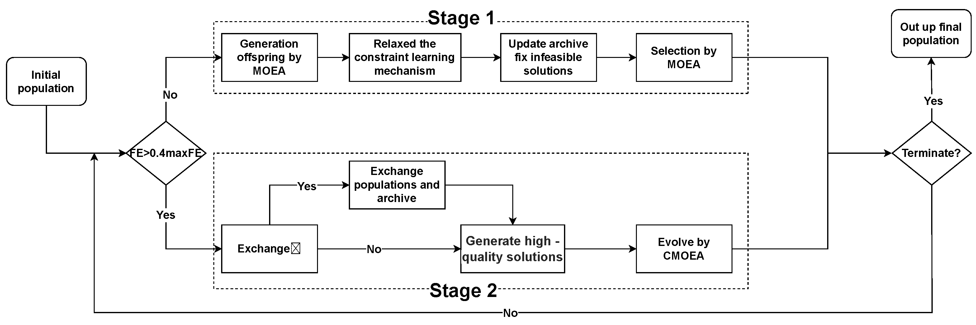
3. The Proposed CMOEA-TA
3.1. Framework of CMOEA-TA
| Algorithm 1 Framework of CMOEA-TA. |
|
3.2. Relaxed the Constraint Learning Mechanism
3.3. The Mechanism of Elite Mating Pool Selection
| Algorithm 2 Elite mating pool selection. |
|
3.4. Updated Archive
| Algorithm 3 UpdatedArchive. |
|
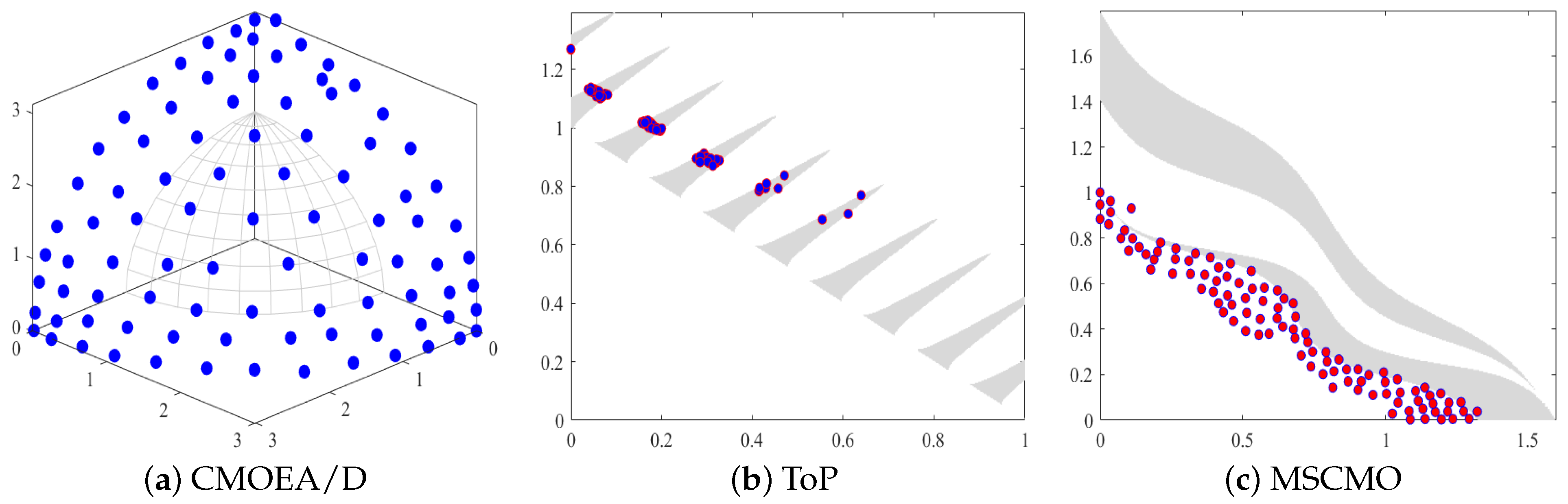
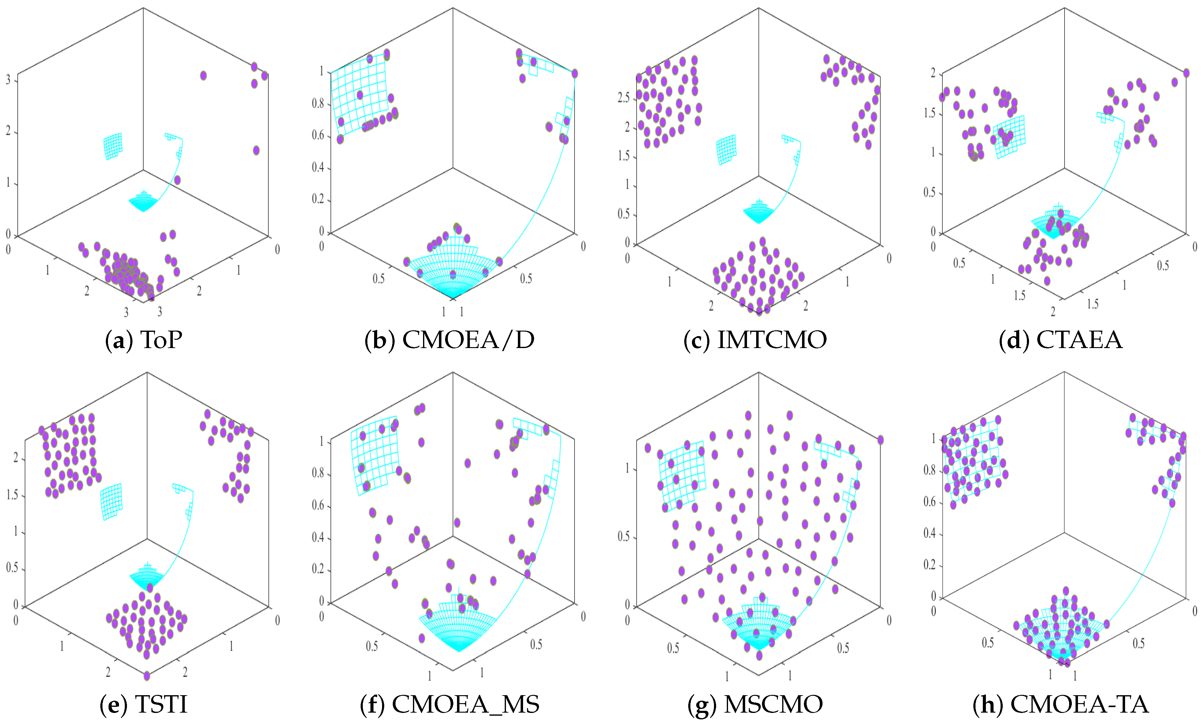
4. Experimental Study
4.1. Experimental Setup
4.2. Comprehensive Analysis of IGD Values
4.3. Comprehensive Analysis of HV Values
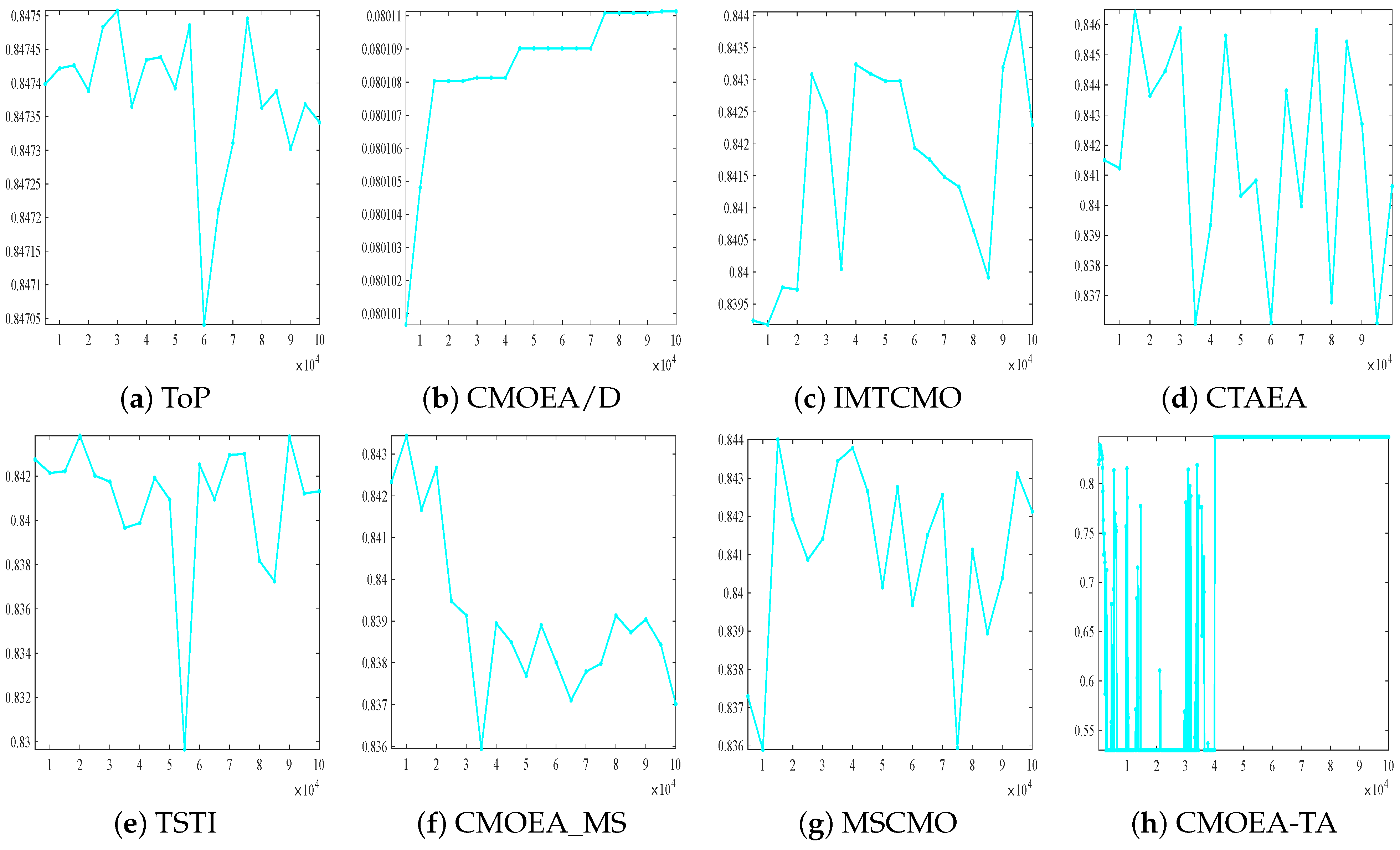
4.4. Performance Analysis
4.5. Real-World Problems Analysis
4.6. Effectiveness of Core Components of CMOEA-TA
5. Conclusions
Author Contributions
Funding
Data Availability Statement
Conflicts of Interest
References
- Zarei, F.; Arashpour, M.; Mirnezami, S.A.; Shahabi-Shahamiri, R.; Ghasemi, M. Multi-skill resource-constrained project scheduling problem considering overlapping: Fuzzy multi-objective programming approach to a case study. Int. J. Constr. Manag. 2024, 24, 820–833. [Google Scholar] [CrossRef]
- Li, X.; Peng, Y.; Tian, Q.; Feng, T.; Wang, W.; Cao, Z.; Song, X. A decomposition-based optimization method for integrated vehicle charging and operation scheduling in automated container terminals under fast charging technology. Transp. Res. Part E Logist. Transp. Rev. 2023, 180, 103338. [Google Scholar] [CrossRef]
- Ding, L.; Shi, C.; Zhou, J. Collaborative route optimization and resource management strategy for multi-target tracking in airborne radar system. Digit. Signal Process. 2023, 138, 104051. [Google Scholar] [CrossRef]
- Farahmand-Tabar, S.; Afrasyabi, P. Multi-modal Routing in Urban Transportation Network Using Multi-objective Quantum Particle Swarm Optimization. In Applied Multi-Objective Optimization; Springer: Berlin/Heidelberg, Germany, 2024; pp. 133–154. [Google Scholar]
- Wang, Q.; Li, T.; Meng, F.; Li, B. A framework for constrained large-scale multi-objective white-box problems based on two-scale optimization through decision transfer. Inf. Sci. 2024, 665, 120411. [Google Scholar] [CrossRef]
- Hao, L.; Peng, W.; Liu, J.; Zhang, W.; Li, Y.; Qin, K. Competition-based two-stage evolutionary algorithm for constrained multi-objective optimization. Math. Comput. Simul. 2025, 230, 207–226. [Google Scholar] [CrossRef]
- Falcón-Cardona, J.G.; Coello, C.A.C. Convergence and diversity analysis of indicator-based multi-objective evolutionary algorithms. In Proceedings of the Genetic and Evolutionary Computation Conference, Prague, Czech Republic, 13–17 July 2019; pp. 524–531. [Google Scholar]
- Wang, F.; Huang, M.; Yang, S.; Wang, X. Penalty and prediction methods for dynamic constrained multi-objective optimization. Swarm Evol. Comput. 2023, 80, 101317. [Google Scholar] [CrossRef]
- Gu, Q.; Liu, R.; Hui, Z.; Wang, D. A constrained multi-objective optimization algorithm based on coordinated strategy of archive and weight vectors. Expert Syst. Appl. 2024, 244, 122961. [Google Scholar] [CrossRef]
- Alwuthaynani, M.M.; Abdallah, Z.S.; Santos-Rodriguez, R. A robust class decomposition-based approach for detecting Alzheimer’s progression. Exp. Biol. Med. 2023, 248, 2514–2525. [Google Scholar] [CrossRef] [PubMed]
- Kawachi, T.; Kushida, J.i.; Hara, A.; Takahama, T. Efficient parameter-free adaptive penalty method with balancing the objective function value and the constraint violation. Int. J. Comput. Intell. Stud. 2021, 10, 127–160. [Google Scholar] [CrossRef]
- Tian, Y.; Zhang, Y.; Su, Y.; Zhang, X.; Tan, K.C.; Jin, Y. Balancing objective optimization and constraint satisfaction in constrained evolutionary multiobjective optimization. IEEE Trans. Cybern. 2021, 52, 9559–9572. [Google Scholar] [CrossRef] [PubMed]
- Zhang, Z.; Zhang, H.; Tian, Y.; Li, C.; Yue, D. Cooperative constrained multi-objective dual-population evolutionary algorithm for optimal dispatching of wind-power integrated power system. Swarm Evol. Comput. 2024, 87, 101525. [Google Scholar] [CrossRef]
- Liu, Z.; Chen, H.; Zhang, T.; Meuser, C.; von Unwerth, T. Multi-Objective Operating Parameters Optimization for the Start Process of Proton Exchange Membrane Fuel Cell Stack with Non-Dominated Sorting Genetic Algorithm II. J. Electrochem. Soc. 2024, 171, 034506. [Google Scholar] [CrossRef]
- Zhou, T.; He, P.; Niu, B.; Yue, G.; Wang, H. A novel competitive constrained dual-archive dual-stage evolutionary algorithm for constrained multiobjective optimization. Swarm Evol. Comput. 2023, 83, 101417. [Google Scholar] [CrossRef]
- Bao, Q.; Wang, M.; Dai, G.; Chen, X.; Song, Z.; Li, S. An archive-based two-stage evolutionary algorithm for constrained multi-objective optimization problems. Swarm Evol. Comput. 2022, 75, 101161. [Google Scholar] [CrossRef]
- Zhong, X.; Yao, X.; Gong, D.; Qiao, K.; Gan, X.; Li, Z. A dual-population-based evolutionary algorithm for multi-objective optimization problems with irregular Pareto fronts. Swarm Evol. Comput. 2024, 87, 101566. [Google Scholar] [CrossRef]
- Lin, J.; Zhang, S.X.; Zheng, S.Y. A diverse/converged individual competition algorithm for computationally expensive many-objective optimization. Appl. Intell. 2024, 54, 2564–2581. [Google Scholar] [CrossRef]
- Su, T.V.; Hang, D.D. Second-order optimality conditions in locally Lipschitz multiobjective fractional programming problem with inequality constraints. Optimization 2023, 72, 1171–1198. [Google Scholar] [CrossRef]
- Fan, C.; Wang, J.; Xiao, L.; Cheng, F.; Ai, Z.; Zeng, Z. A coevolution algorithm based on two-staged strategy for constrained multi-objective problems. Appl. Intell. 2022, 52, 17954–17973. [Google Scholar] [CrossRef]
- Yeste, P.; Melsen, L.A.; García-Valdecasas Ojeda, M.; Gámiz-Fortis, S.R.; Castro-Díez, Y.; Esteban-Parra, M.J. A Pareto-Based Sensitivity Analysis and Multiobjective Calibration Approach for Integrating Streamflow and Evaporation Data. Water Resour. Res. 2023, 59, e2022WR033235. [Google Scholar] [CrossRef]
- Liu, Z.Z.; Wang, Y. Handling constrained multiobjective optimization problems with constraints in both the decision and objective spaces. IEEE Trans. Evol. Comput. 2019, 23, 870–884. [Google Scholar] [CrossRef]
- Fan, Z.; Li, W.; Cai, X.; Li, H.; Wei, C.; Zhang, Q.; Deb, K.; Goodman, E. Push and pull search for solving constrained multi-objective optimization problems. Swarm Evol. Comput. 2019, 44, 665–679. [Google Scholar] [CrossRef]
- Jain, H.; Deb, K. An evolutionary many-objective optimization algorithm using reference-point based nondominated sorting approach, part II: Handling constraints and extending to an adaptive approach. IEEE Trans. Evol. Comput. 2013, 18, 602–622. [Google Scholar] [CrossRef]
- Ma, H.; Wei, H.; Tian, Y.; Cheng, R.; Zhang, X. A multi-stage evolutionary algorithm for multi-objective optimization with complex constraints. Inf. Sci. 2021, 560, 68–91. [Google Scholar] [CrossRef]
- Tian, Y.; Zhang, T.; Xiao, J.; Zhang, X.; Jin, Y. A coevolutionary framework for constrained multiobjective optimization problems. IEEE Trans. Evol. Comput. 2020, 25, 102–116. [Google Scholar] [CrossRef]
- Ming, F.; Gong, W.; Gao, L. Adaptive auxiliary task selection for multitasking-assisted constrained multi-objective optimization [feature]. IEEE Comput. Intell. Mag. 2023, 18, 18–30. [Google Scholar] [CrossRef]
- Wang, J.; Liang, G.; Zhang, J. Cooperative differential evolution framework for constrained multiobjective optimization. IEEE Trans. Cybern. 2018, 49, 2060–2072. [Google Scholar] [CrossRef]
- Li, K.; Chen, R.; Fu, G.; Yao, X. Two-archive evolutionary algorithm for constrained multiobjective optimization. IEEE Trans. Evol. Comput. 2018, 23, 303–315. [Google Scholar] [CrossRef]
- Ming, F.; Gong, W.; Zhen, H.; Li, S.; Wang, L.; Liao, Z. A simple two-stage evolutionary algorithm for constrained multi-objective optimization. Knowl.-Based Syst. 2021, 228, 107263. [Google Scholar] [CrossRef]
- Li, Y.; Feng, X.; Yu, H. A constrained multiobjective evolutionary algorithm with the two-archive weak cooperation. Inf. Sci. 2022, 615, 415–430. [Google Scholar] [CrossRef]
- Qiao, K.; Liang, J.; Yu, K.; Yue, C.; Lin, H.; Zhang, D.; Qu, B. Evolutionary constrained multiobjective optimization: Scalable high-dimensional constraint benchmarks and algorithm. IEEE Trans. Evol. Comput. 2023, 28, 965–979. [Google Scholar] [CrossRef]
- Yu, K.; Liang, J.; Qu, B.; Luo, Y.; Yue, C. Dynamic selection preference-assisted constrained multiobjective differential evolution. IEEE Trans. Syst. Man Cybern. Syst. 2021, 52, 2954–2965. [Google Scholar] [CrossRef]
- Dong, J.; Gong, W.; Ming, F.; Wang, L. A two-stage evolutionary algorithm based on three indicators for constrained multi-objective optimization. Expert Syst. Appl. 2022, 195, 116499. [Google Scholar] [CrossRef]
- Hakimazari, M.; Baghoolizadeh, M.; Sajadi, S.M.; Kheiri, P.; Moghaddam, M.Y.; Rostamzadeh-Renani, M.; Rostamzadeh-Renani, R.; Hamooleh, M.B. Multi-objective optimization of daylight illuminance indicators and energy usage intensity for office space in Tehran by genetic algorithm. Energy Rep. 2024, 11, 3283–3306. [Google Scholar] [CrossRef]
- Shen, X.; Yao, X.; Gong, D.; Tu, H. Multi-objective optimization and integrated indicator-driven two-stage project recommendation in time-dependent software ecosystem. Inf. Softw. Technol. 2024, 170, 107433. [Google Scholar] [CrossRef]
- Zhu, Q.; Zhang, Q.; Lin, Q. A constrained multiobjective evolutionary algorithm with detect-and-escape strategy. IEEE Trans. Evol. Comput. 2020, 24, 938–947. [Google Scholar] [CrossRef]
- Ma, Z.; Wang, Y.; Song, W. A new fitness function with two rankings for evolutionary constrained multiobjective optimization. IEEE Trans. Syst. Man Cybern. Syst. 2019, 51, 5005–5016. [Google Scholar] [CrossRef]
- Zhou, Y.; Zhu, M.; Wang, J.; Zhang, Z.; Xiang, Y.; Zhang, J. Tri-goal evolution framework for constrained many-objective optimization. IEEE Trans. Syst. Man Cybern. Syst. 2018, 50, 3086–3099. [Google Scholar] [CrossRef]
- Liu, Z.Z.; Wang, Y.; Wang, B.C. Indicator-based constrained multiobjective evolutionary algorithms. IEEE Trans. Syst. Man Cybern. Syst. 2019, 51, 5414–5426. [Google Scholar] [CrossRef]
- Cetina-Quiñones, A.; Bassam, A.; Medina-Carril, D.; Chan-Dzib, E.; Hernandez Bautista, A. Multi-objective optimization of energo-enviro-economic indicators of an outdoor swimming pool heating system: An approach with advanced computational techniques. J. Braz. Soc. Mech. Sci. Eng. 2024, 46, 186. [Google Scholar] [CrossRef]
- Zitzler, E.; Laumanns, M.; Thiele, L. SPEA2: Improving the strength Pareto evolutionary algorithm. TIK Report. 2001, 103. [Google Scholar] [CrossRef]
- Jin, L.; Kazemi, M.; Comodi, G.; Papadimitriou, C. Assessing battery degradation as a key performance indicator for multi-objective optimization of multi-carrier energy systems. Appl. Energy 2024, 361, 122925. [Google Scholar] [CrossRef]
- Xie, Y.; Li, J.; Li, Y.; Zhu, W.; Dai, C. Two-stage evolutionary algorithm with fuzzy preference indicator for multimodal multi-objective optimization. Swarm Evol. Comput. 2024, 85, 101480. [Google Scholar] [CrossRef]
- Yuan, J.; Liu, H.L.; Yang, S. An adaptive parental guidance strategy and its derived indicator-based evolutionary algorithm for multi-and many-objective optimization. Swarm Evol. Comput. 2024, 84, 101449. [Google Scholar] [CrossRef]
- Desai, S.A.; Monika, s. An empirical study on application of Wilcoxon signed rank test in statistical process control when process target is fixed. Int. J. Manag. IT Eng. 2018, 8, 130–136. [Google Scholar]
- Tian, Y.; Zhu, W.; Zhang, X.; Jin, Y. A practical tutorial on solving optimization problems via PlatEMO. Neurocomputing 2023, 518, 190–205. [Google Scholar] [CrossRef]

| Abbreviation | Full Form |
|---|---|
| CMOP [5] | Constrained Multi-objective Optimization Problems |
| MOEA | Multi-objective Evolutionary Algorithms |
| CMOEA [6] | Constrained Multi-objective Evolutionary Algorithms |
| CMOEA-TA | Two-stage Archiving Constrained Multi-objective Evolutionary Algorithms |
| ToP [22] | Two-phase Optimization Procedure |
| PPS [23] | Push and Pull Search |
| CMOEA-MS [12] | Constrained Multi-Objective Evolutionary Algorithm with Multiple Strategies |
| CMOEA/D [24] | Constrained Multi-Objective Evolutionary Algorithm based on Decomposition |
| MSCMO [25] | Multi-Stage Constrained Multi-Objective |
| CCMO [26] | Coevolutionary Constrained Multiobjective Optimization |
| CMOQLMT [27] | Constrained Multi-Objective Quadratic Learning-based Multi-task |
| CCMODE [28] | Cooperative Constrained Multi-Objective Differential Evolution |
| C-TAEA [29] | Constrained Two-Archive Evolutionary Algorithm |
| C-TSEA [30] | Constrained Two-Stage Evolutionary Algorithm |
| CMOEA-TWC [31] | Constrained Multiobjective Evolutionary Algorithm with Two-Archive Weak Cooperation |
| IMTCMO [32] | Infeasibility-based Multi-Task Constrained Multi-Objective Optimization |
| DSPCMDE [33] | Dynamic Selection Preference-Assisted Constrained Multiobjective Differential Evolution |
| TSTI [34] | Two-Stage Three-Indicator |
| SPEA | Strength Pareto Evolutionary Algorithm |
| GA | Genetic Algorithm |
| SO | Swarm Optimization |
| PF [21] | Pareto Front |
| CPF [17] | Constrained Pareto Front |
| CV | Constraint Violation |
| CDP | Constraint Dominance Principle |
| FE | Function Evaluations |
| Feasible Ratio | |
| IGD [35] | Inverse Generation Distance |
| HV [36] | HyperVolume |
| Problem | M | D | CMOEA/D | ToP | TSTI | MSCMO | CMOEA_MS | CTAEA | IMTCMO | CMOEA-TA |
|---|---|---|---|---|---|---|---|---|---|---|
| MW1 | 2 | 15 | 2.3584e-2 (6.07e-2) − | NaN (NaN) | 5.1794e-3 (9.85e-3) ≈ | 1.8263e-2 (3.83e-2) − | 4.2037e-2 (6.54e-2) − | 3.3830e-2 (3.48e-2) − | 1.7055e-3 (2.97e-5) + | 1.8848e-3 (1.21e-3) |
| MW2 | 2 | 15 | 2.1518e-2 (7.13e-3) ≈ | 1.7940e-1 (1.48e-1) − | 1.7211e-2 (6.63e-3) ≈ | 2.2471e-2 (7.64e-3) ≈ | 2.4023e-2 (8.46e-3) ≈ | 1.8133e-2 (7.89e-3) ≈ | 5.9994e-2 (3.53e-2) − | 2.0670e-2 (9.10e-3) |
| MW3 | 2 | 15 | 5.6961e-3 (6.97e-4) − | 2.2097e-1 (3.23e-1) − | 1.8927e-2 (3.28e-2) − | 5.0488e-2 (1.37e-3) − | 1.3648e-2 (5.31e-3) − | 1.2954e-2 (2.52e-3) − | 4.8148e-3 (1.13e-4) ≈ | 4.8462e-3 (1.91e-4) |
| MW4 | 3 | 15 | 4.1786e-2 (1.00e-3) − | 7.2571e-1 (0.00e+0) ≈ | 4.1814e-2 (1.13e-3) − | 6.1061e-2 (2.08e-2) − | 4.9339e-2 (7.63e-3) − | 6.4495e-2 (2.06e-2) − | 4.8393e-2 (1.35e-2) − | 4.0495e-2 (4.23e-4) |
| MW5 | 2 | 15 | 1.9579e-3 (1.83e-3) − | 7.5416e-1 (0.00e+0) ≈ | 5.8355e-2 (1.62e-1) − | 3.2066e-2 (1.18e-1) − | 6.9010e-2 (1.22e-1) − | 1.4127e-2 (4.15e-3) − | 1.8159e-3 (5.34e-4) − | 6.9501e-4 (6.65e-4) |
| MW6 | 2 | 15 | 1.8220e-2 (1.07e-2) ≈ | 7.3029e-1 (3.51e-1) − | 6.3375e-2 (1.30e-1) ≈ | 2.3689e-2 (1.13e-2) ≈ | 1.7844e-1 (2.16e-1) − | 1.0959e-2 (6.47e-3) + | 1.5146e-1 (1.88e-1) − | 2.4049e-2 (1.20e-2) |
| MW7 | 2 | 15 | 2.7204e-2 (1.00e-1) − | 5.7367e-2 (9.94e-2) − | 4.5487e-3 (4.55e-4) − | 4.4436e-3 (3.77e-4) − | 3.1495e-2 (2.92e-2) − | 6.7262e-3 (5.04e-4) − | 4.3318e-3 (2.04e-4) − | 4.1605e-3 (2.18e-4) |
| MW8 | 3 | 15 | 5.7801e-2 (1.92e-2) − | 6.9878e-1 (4.11e-1) − | 5.0807e-2 (9.62e-3) − | 5.1137e-2 (6.93e-3) − | 5.2374e-2 (1.45e-2) − | 5.4905e-2 (3.09e-3) − | 7.4128e-2 (3.75e-2) − | 4.4684e-2 (2.16e-3) |
| MW9 | 2 | 15 | 1.1867e-2 (1.21e-2) − | 8.5441e-1 (8.52e-2) − | 6.5016e-2 (1.80e-1) − | 7.5498e-2 (2.17e-1) − | 2.0160e-1 (2.60e-1) − | 8.7774e-3 (1.69e-3) − | 5.5130e-3 (9.16e-4) − | 4.3101e-3 (1.66e-4) |
| MW10 | 2 | 15 | 1.2514e-1 (1.73e-1) ≈ | NaN (NaN) | 9.0594e-2 (1.29e-1) ≈ | 1.1679e-1 (1.85e-1) ≈ | 3.6383e-2 (1.90e-2) ≈ | 2.6026e-2 (1.65e-2) ≈ | 1.7727e-1 (5.62e-2) − | 1.2531e-1 (2.14e-1) |
| MW11 | 2 | 15 | 8.1605e-2 (2.11e-1) − | 5.2819e-1 (2.69e-1) − | 6.0490e-3 (1.34e-4) ≈ | 6.0964e-3 (1.20e-4) ≈ | 1.4053e-2 (1.01e-2) − | 2.0545e-2 (7.72e-3) − | 5.9456e-3 (1.35e-4) + | 6.0524e-3 (1.07e-4) |
| MW12 | 2 | 15 | 5.2969e-3 (1.87e-3) + | 8.3690e-1 (0.00e+0) ≈ | 4.8703e-3 (3.82e-4) ≈ | 9.0572e-2 (2.39e-1) ≈ | 1.5524e-1 (2.82e-1) − | 6.1014e-2 (1.82e-1) − | 4.7654e-3 (1.32e-4) ≈ | 4.3137e-2 (1.72e-1) |
| MW13 | 2 | 15 | 1.4945e-1 (3.06e-1) − | 1.0845e+0 (7.97e-1) − | 1.1491e-1 (5.46e-2) − | 1.2221e-1 (6.58e-2) − | 5.0814e-1 (4.96e-1) − | 6.3400e-2 (3.47e-2) ≈ | 1.6385e-1 (9.68e-2) − | 5.6480e-2 (3.29e-2) |
| MW14 | 3 | 15 | 2.1253e-1 (1.58e-3) − | 8.5539e-1 (8.65e-1) − | 9.9443e-2 (3.47e-3) − | 2.6988e-1 (2.13e-1) − | 3.2031e-1 (1.88e-1) − | 4.9614e-1 (3.99e-1) − | 9.9032e-2 (1.80e-3) − | 9.6494e-2 (1.31e-3) |
| 1/10/3 | 0/9/3 | 0/8/6 | 0/9/5 | 0/12/2 | 1/10/3 | 2/10/2 | ||||
| LIRCMOP1 | 2 | 30 | 2.6605e-1 (3.37e-2) − | 3.2853e-1 (2.16e-2) − | 2.1023e-1 (1.61e-2) − | 1.7366e-1 (6.64e-2) ≈ | 3.2481e-1 (4.71e-2) − | 3.0813e-1 (9.45e-2) − | 2.6521e-2 (8.07e-3) + | 1.5082e-1 (3.57e-2) |
| LIRCMOP2 | 2 | 30 | 2.4059e-1 (3.20e-2) − | 2.8906e-1 (2.18e-2) − | 1.9674e-1 (2.60e-2) − | 1.7570e-1 (4.37e-2) − | 2.7883e-1 (4.45e-2) − | 2.4246e-1 (9.34e-2) − | 1.9316e-1 (4.29e-2) − | 1.3974e-1 (3.25e-2) |
| LIRCMOP3 | 2 | 30 | 2.9268e-1 (4.09e-2) − | 3.4399e-1 (1.64e-2) − | 2.2665e-1 (2.50e-2) − | 1.7748e-1 (7.59e-2) ≈ | 3.2129e-1 (4.27e-2) − | 3.4241e-1 (1.64e-1) − | 1.5362e-2 (7.41e-3) + | 1.4615e-1 (2.23e-2) |
| LIRCMOP4 | 2 | 30 | 2.7739e-1 (2.83e-2) − | 3.2278e-1 (1.21e-2) − | 2.2184e-1 (2.40e-2) − | 1.7877e-1 (6.06e-2) ≈ | 2.7799e-1 (4.96e-2) − | 2.9330e-1 (5.13e-2) − | 2.1581e-1 (4.24e-2) − | 1.7325e-1 (2.87e-2) |
| LIRCMOP5 | 2 | 30 | 1.3606e+0 (4.15e-1) − | 1.1161e+0 (2.81e-1) − | 9.5232e-1 (4.14e-1) − | 7.1017e-1 (1.20e+0) − | 3.7233e-1 (2.04e-1) − | 1.2229e+0 (2.19e-1) − | 1.6409e+0 (5.60e-1) − | 2.6910e-1 (6.15e-2) |
| LIRCMOP6 | 2 | 30 | 1.3462e+0 (4.96e-4) − | 1.3467e+0 (4.70e-4) − | 1.0774e+0 (4.22e-1) − | 5.6711e-1 (4.75e-1) − | 5.0159e-1 (3.69e-1) − | 1.4359e+0 (3.20e-1) − | 3.9458e-1 (4.69e-1) ≈ | 2.7307e-1 (1.03e-1) |
| LIRCMOP7 | 2 | 30 | 1.2294e+0 (7.10e-1) − | 1.3804e+0 (6.23e-1) − | 1.3641e-1 (3.25e-2) − | 1.2684e-1 (5.15e-2) ≈ | 1.3986e-1 (3.98e-2) − | 8.2863e-1 (7.43e-1) − | 3.0093e-2 (4.74e-2) + | 1.0432e-1 (2.42e-2) |
| LIRCMOP8 | 2 | 30 | 1.5407e+0 (4.37e-1) − | 1.5448e+0 (4.26e-1) − | 3.8337e-1 (4.46e-1) − | 2.0599e-1 (5.03e-2) − | 1.9733e-1 (3.83e-2) − | 1.3794e+0 (7.07e-1) − | 3.6623e-2 (5.69e-2) + | 1.4401e-1 (5.24e-2) |
| LIRCMOP9 | 2 | 30 | 8.6590e-1 (1.40e-1) − | 5.9781e-1 (1.38e-1) − | 5.1760e-1 (5.28e-2) − | 5.4604e-1 (2.37e-1) ≈ | 6.9448e-1 (1.45e-1) − | 8.1715e-1 (2.97e-1) − | 3.7098e-1 (7.51e-2) + | 4.4033e-1 (9.00e-2) |
| LIRCMOP10 | 2 | 30 | 8.0151e-1 (1.49e-1) − | 4.2407e-1 (5.83e-2) − | 6.0129e-1 (2.28e-1) − | 2.6753e-1 (1.36e-1) − | 4.7126e-1 (1.46e-1) − | 7.2617e-1 (4.02e-1) − | 2.2463e-2 (4.56e-2) + | 1.7029e-1 (6.94e-2) |
| LIRCMOP11 | 2 | 30 | 8.8053e-1 (7.32e-2) − | 4.7327e-1 (1.14e-1) − | 5.9713e-1 (1.50e-1) − | 1.6791e-1 (1.34e-1) − | 3.5132e-1 (1.61e-1) − | 6.2374e-1 (4.03e-1) − | 1.1186e-1 (9.19e-2) ≈ | 7.9458e-2 (4.69e-2) |
| LIRCMOP12 | 2 | 30 | 6.8445e-1 (1.79e-1) − | 3.1726e-1 (7.74e-2) − | 3.4999e-1 (8.22e-2) − | 4.1603e-1 (1.96e-1) − | 3.9776e-1 (1.40e-1) − | 6.5436e-1 (4.89e-1) − | 1.7933e-1 (4.18e-2) ≈ | 2.2480e-1 (9.26e-2) |
| LIRCMOP13 | 3 | 30 | 1.3034e+0 (2.63e-4) − | 1.3129e+0 (9.95e-2) − | 1.1956e+0 (3.75e-1) − | 9.6046e-2 (2.33e-3) ≈ | 9.4959e-2 (2.80e-3) ≈ | 7.2146e-1 (6.26e-1) − | 1.3102e+0 (1.54e-3) − | 9.4648e-2 (1.17e-3) |
| LIRCMOP14 | 3 | 30 | 1.2595e+0 (2.97e-4) − | 1.3028e+0 (6.03e-3) − | 1.2719e+0 (1.85e-3) − | 9.7539e-2 (2.42e-3) − | 9.7374e-2 (2.81e-3) ≈ | 1.1114e-1 (1.37e-3) − | 1.2842e+0 (4.32e-3) − | 9.5547e-2 (9.27e-4) |
| 0/14/0 | 0/14/0 | 0/14/0 | 0/8/6 | 0/12/2 | 0/14/0 | 6/5/3 | ||||
| ZXH_CF1 | 3 | 13 | 4.4992e-2 (8.92e-4) + | 9.7660e-2 (1.56e-2) − | 4.6274e-2 (8.80e-4) + | 4.9205e-2 (8.82e-4) − | 4.9308e-2 (1.25e-3) − | 4.8756e-2 (1.50e-3) − | 5.4677e-2 (1.77e-3) − | 4.7450e-2 (9.62e-4) |
| ZXH_CF2 | 3 | 13 | 1.3602e-1 (2.14e-1) − | 3.1536e-1 (1.70e-1) − | 1.1518e-1 (1.49e-1) − | 1.7290e-1 (2.02e-1) ≈ | 1.4038e-1 (2.63e-1) ≈ | 9.6657e-2 (8.65e-2) + | 6.0289e-2 (1.06e-3) + | 9.9641e-2 (1.40e-1) |
| ZXH_CF3 | 3 | 13 | 7.4126e-2 (2.04e-3) − | 2.2845e-1 (5.99e-2) − | 6.1754e-2 (1.43e-3) ≈ | 7.8090e-2 (1.78e-2) − | 8.2462e-2 (3.86e-3) − | 7.5642e-2 (2.67e-3) − | 8.0494e-2 (2.65e-3) − | 6.2459e-2 (1.16e-3) |
| ZXH_CF4 | 3 | 13 | 1.3128e-1 (9.08e-2) ≈ | 1.2052e+0 (2.55e-1) − | 2.1409e-1 (2.62e-1) ≈ | 1.4814e-1 (1.13e-1) ≈ | 2.5642e-1 (3.04e-1) ≈ | 1.1208e-1 (6.64e-2) ≈ | 3.0602e-1 (4.02e-1) ≈ | 1.8278e-1 (1.43e-1) |
| ZXH_CF5 | 3 | 13 | 8.3063e-2 (1.22e-1) − | 1.1952e-1 (5.06e-2) − | 1.6079e-1 (2.42e-1) ≈ | 1.8633e-1 (2.35e-1) − | 1.5666e-1 (3.91e-1) − | 5.7842e-2 (3.25e-2) + | 3.6755e-2 (6.76e-4) + | 7.6004e-2 (1.41e-1) |
| ZXH_CF6 | 3 | 13 | 5.1424e-2 (1.64e-3) − | 5.6768e-2 (7.17e-3) − | 3.1093e-2 (7.51e-4) ≈ | 3.7145e-2 (1.53e-2) − | 3.3786e-2 (9.61e-4) − | 3.6313e-2 (1.60e-3) − | 3.4249e-2 (8.42e-4) − | 3.1484e-2 (6.36e-4) |
| ZXH_CF7 | 3 | 13 | 1.1754e-1 (8.18e-2) − | 5.5079e-1 (2.46e-1) − | 1.6633e-1 (9.83e-2) − | 3.5776e-1 (2.13e-1) − | 2.6985e-1 (2.08e-1) − | 9.3481e-2 (6.01e-2) − | 1.9554e-1 (2.42e-1) − | 7.1806e-2 (7.68e-2) |
| ZXH_CF8 | 3 | 13 | 6.3914e-2 (4.64e-3) − | 2.4528e-1 (3.62e-1) − | 3.1273e-2 (4.59e-4) + | 2.3968e-1 (1.34e-1) − | 1.5169e-1 (2.76e-2) − | 5.6277e-2 (5.62e-3) − | 4.2737e-2 (1.05e-3) − | 3.1794e-2 (6.94e-4) |
| ZXH_CF9 | 3 | 13 | 9.8523e-2 (6.10e-2) − | 5.1171e-1 (1.21e-1) − | 2.6399e-2 (5.85e-4) + | 7.4746e-2 (3.12e-2) − | 1.4279e-1 (1.06e-1) − | 6.5038e-2 (1.40e-2) − | 2.9977e-2 (7.86e-4) − | 2.6735e-2 (4.45e-4) |
| ZXH_CF10 | 3 | 13 | 2.2796e-1 (2.55e-1) − | 1.1566e+0 (4.25e-1) − | 1.3016e-1 (1.00e-1) ≈ | 1.9627e-1 (1.66e-1) − | 3.6530e-1 (3.20e-1) − | 1.2220e-1 (8.04e-2) − | 1.9639e-1 (1.98e-1) − | 6.9362e-2 (7.11e-2) |
| ZXH_CF11 | 3 | 13 | 1.1475e-1 (1.00e-1) − | 5.1396e-1 (2.09e-1) − | 2.8028e-2 (4.51e-4) ≈ | 9.0487e-2 (2.33e-2) − | 2.9348e-2 (3.45e-4) − | 3.5532e-2 (9.70e-4) − | 2.8493e-2 (3.77e-4) − | 2.8123e-2 (4.54e-4) |
| ZXH_CF12 | 3 | 13 | 2.2195e-1 (2.05e-1) − | 4.8357e-1 (1.01e-1) − | 1.7894e-1 (3.07e-1) ≈ | 2.0889e-1 (3.48e-1) − | 1.0819e-1 (2.19e-1) − | 7.5879e-2 (1.50e-1) − | 2.5987e-2 (8.12e-4) + | 7.1211e-2 (1.17e-1) |
| ZXH_CF13 | 2 | 12 | 8.9725e-2 (1.49e-1) ≈ | 9.5274e-1 (3.91e-1) − | 3.3227e-1 (3.33e-1) ≈ | 2.0733e-1 (3.29e-1) ≈ | 3.2273e-1 (2.31e-1) ≈ | 7.4464e-2 (1.04e-1) ≈ | 1.7974e-1 (2.36e-1) ≈ | 3.2395e-1 (4.67e-1) |
| ZXH_CF14 | 2 | 12 | 7.9689e-3 (1.83e-2) − | 1.4504e-1 (2.09e-1) − | 2.3831e-3 (5.13e-5) − | 2.3952e-3 (5.04e-5) − | 2.5264e-3 (5.04e-5) − | 2.8541e-3 (1.22e-4) − | 3.1063e-3 (7.60e-4) − | 2.3435e-3 (3.74e-5) |
| ZXH_CF15 | 2 | 12 | 9.8882e-2 (1.54e-1) − | 1.8225e-1 (2.06e-1) − | 3.8100e-2 (1.25e-1) ≈ | 1.5372e-1 (3.10e-1) ≈ | 2.6988e-2 (5.14e-2) − | 5.6692e-3 (7.02e-4) + | 2.9271e-3 (7.37e-5) + | 2.6042e-2 (1.04e-1) |
| ZXH_CF16 | 2 | 12 | 7.4565e-2 (4.78e-2) − | 2.7397e-2 (4.87e-2) − | 2.6260e-3 (3.94e-5) ≈ | 2.6375e-3 (3.60e-5) ≈ | 8.3846e-2 (5.56e-2) − | 1.4255e-2 (5.13e-3) − | 2.7845e-3 (5.03e-5) − | 2.6406e-3 (5.53e-5) |
| 1/13/2 | 0/16/0 | 3/3/10 | 0/11/5 | 0/13/3 | 3/11/2 | 4/10/2 | ||||
| C1_DTLZ1 | 3 | 7 | 2.0506e-2 (4.33e-5) − | NaN (NaN) | 2.0642e-2 (5.89e-4) − | 2.0558e-2 (5.80e-4) − | 2.1095e-2 (5.92e-4) − | 2.3158e-2 (3.07e-4) − | 2.1200e-2 (2.82e-4) − | 2.0057e-2 (1.11e-4) |
| C1_DTLZ3 | 3 | 12 | 2.4951e+0 (3.71e+0) − | 2.6077e-1 (4.37e-1) − | 6.0234e+0 (3.54e+0) − | 4.5386e-1 (1.78e+0) ≈ | 5.4781e-2 (1.54e-3) ≈ | 9.4902e-2 (1.13e-1) − | 6.0441e+0 (3.50e+0) − | 5.4517e-2 (9.98e-4) |
| C2_DTLZ2 | 3 | 12 | 4.9310e-2 (2.24e-5) − | 1.1085e-1 (2.15e-1) − | 4.3699e-2 (1.29e-3) − | 4.3685e-2 (1.09e-3) − | 4.3628e-2 (1.44e-3) − | 5.6604e-2 (1.15e-3) − | 4.5503e-2 (5.78e-4) − | 4.2557e-2 (5.74e-4) |
| C3_DTLZ4 | 3 | 12 | 9.1366e-2 (5.18e-5) + | 1.4350e-1 (6.45e-3) − | 9.8652e-2 (2.79e-3) − | 1.7608e-1 (2.34e-1) ≈ | 6.5367e-1 (5.54e-2) − | 1.1172e-1 (2.04e-3) − | 9.7809e-2 (1.77e-3) − | 9.6124e-2 (1.29e-3) |
| DC1_DTLZ1 | 3 | 7 | 1.9407e-2 (4.59e-3) − | 2.0815e-2 (6.46e-3) − | 4.5110e-2 (1.03e-1) ≈ | 1.7235e-2 (9.70e-3) − | 1.5678e-2 (5.65e-3) − | 3.0898e-2 (7.01e-2) − | 1.2287e-2 (2.82e-4) − | 1.1587e-2 (1.00e-4) |
| DC1_DTLZ3 | 3 | 12 | 4.5090e-2 (2.41e-5) − | 8.1687e-1 (1.80e+0) − | 3.4721e-2 (1.10e-3) ≈ | 2.0176e-1 (2.66e-1) − | 5.0509e-2 (7.16e-2) ≈ | 4.3182e-2 (1.39e-3) − | 3.4730e-2 (5.00e-4) − | 3.4227e-2 (4.74e-4) |
| DC2_DTLZ1 | 3 | 7 | 7.1076e-2 (7.01e-2) − | NaN (NaN) | 5.6862e-2 (6.41e-2) − | 2.0659e-2 (5.52e-4) − | 2.1261e-2 (5.66e-4) − | 2.3208e-2 (1.88e-4) − | 3.0650e-2 (3.26e-2) − | 2.0124e-2 (1.35e-4) |
| DC2_DTLZ3 | 3 | 12 | 5.6089e-1 (3.52e-4) − | NaN (NaN) | 5.6291e-1 (0.00e+0) ≈ | 2.4699e-1 (2.31e-1) − | 4.6031e-1 (2.09e-1) − | 1.6441e-1 (1.99e-1) − | 5.6882e-1 (2.66e-3) − | 5.3494e-2 (5.50e-4) |
| DC3_DTLZ1 | 3 | 7 | 1.2063e-1 (9.61e-2) − | 1.4582e+0 (2.19e+0) − | 2.7795e-1 (2.04e-1) − | 3.9023e-2 (3.54e-2) − | 3.5516e-2 (9.15e-3) − | 9.3686e-3 (3.19e-4) − | 4.5143e-2 (6.85e-2) − | 6.9870e-3 (6.58e-5) |
| DC3_DTLZ3 | 3 | 12 | 1.1580e+0 (5.25e-1) − | 6.8777e+0 (4.29e+0) − | 1.8928e+0 (4.20e-1) − | 8.6087e-1 (8.62e-1) − | 2.6288e-1 (4.10e-1) − | 2.6743e-2 (1.03e-3) + | 1.0104e+0 (3.75e-1) − | 4.7247e-2 (1.20e-1) |
| 1/9/0 | 0/7/0 | 0/7/3 | 0/8/2 | 0/8/2 | 1/9/0 | 0/10/0 | ||||
| 3/46/5 | 0/46/3 | 3/32/19 | 0/36/18 | 0/45/9 | 5/44/5 | 12/35/7 | ||||
| Problem | M | D | CMOEA/D | ToP | TSTI | MSCMO | CMOEA_MS | CTAEA | IMTCMO | CMOEA-TA |
|---|---|---|---|---|---|---|---|---|---|---|
| MW1 | 2 | 15 | 4.6948e-1 (5.16e-2) − | NaN (NaN) | 4.8487e-1 (1.16e-2) ≈ | 4.6877e-1 (3.66e-2) − | 4.4701e-1 (5.90e-2) − | 4.4028e-1 (5.14e-2) − | 4.8951e-1 (6.92e-5) − | 4.8956e-1 (2.46e-3) |
| MW2 | 2 | 15 | 5.5149e-1 (1.16e-2) ≈ | 3.7181e-1 (1.54e-1) − | 5.5898e-1 (1.12e-2) ≈ | 5.5054e-1 (1.29e-2) ≈ | 5.4790e-1 (1.25e-2) ≈ | 5.5749e-1 (1.36e-2) ≈ | 4.9835e-1 (4.47e-2) − | 5.5353e-1 (1.41e-2) |
| MW3 | 2 | 15 | 5.4375e-1 (8.97e-4) − | 3.8019e-1 (1.79e-1) − | 5.3354e-1 (2.24e-2) ≈ | 5.2723e-1 (2.02e-3) − | 5.3372e-1 (6.42e-3) − | 5.3036e-1 (5.69e-3) − | 5.4446e-1 (1.83e-4) ≈ | 5.4434e-1 (4.67e-4) |
| MW4 | 3 | 15 | 8.4106e-1 (8.60e-4) − | 1.1720e-1 (0.00e+0) ≈ | 8.4078e-1 (9.66e-4) − | 8.1638e-1 (2.74e-2) − | 8.2816e-1 (1.25e-2) − | 8.0781e-1 (3.59e-2) − | 8.2920e-1 (1.99e-2) − | 8.4186e-1 (3.92e-4) |
| MW5 | 2 | 15 | 3.2393e-1 (5.91e-4) − | 5.6763e-2 (0.00e+0) ≈ | 3.0222e-1 (5.04e-2) − | 3.1332e-1 (3.41e-2) − | 2.9085e-1 (3.74e-2) − | 3.1575e-1 (3.06e-3) − | 3.2350e-1 (3.57e-4) − | 3.2439e-1 (1.99e-4) |
| MW6 | 2 | 15 | 3.0532e-1 (1.52e-2) ≈ | 7.1210e-2 (5.91e-2) − | 2.8970e-1 (4.04e-2) ≈ | 2.9767e-1 (1.54e-2) ≈ | 2.5440e-1 (6.20e-2) − | 3.1273e-1 (9.65e-3) + | 2.3016e-1 (6.84e-2) − | 2.9732e-1 (1.65e-2) |
| MW7 | 2 | 15 | 4.0276e-1 (3.74e-2) − | 3.7013e-1 (3.75e-2) − | 4.1225e-1 (3.60e-4) − | 4.1204e-1 (7.67e-4) − | 3.9918e-1 (2.22e-2) − | 4.0939e-1 (6.45e-4) − | 4.1218e-1 (2.20e-4) − | 4.1257e-1 (3.42e-4) |
| MW8 | 3 | 15 | 5.1728e-1 (4.40e-2) − | 1.2738e-1 (1.54e-1) − | 5.2085e-1 (2.46e-2) − | 5.1916e-1 (1.92e-2) − | 5.2514e-1 (1.37e-2) − | 5.1979e-1 (1.35e-2) − | 4.6974e-1 (6.71e-2) − | 5.3614e-1 (9.65e-3) |
| MW9 | 2 | 15 | 3.8407e-1 (1.20e-2) − | 0.0000e+0 (0.00e+0) − | 3.5869e-1 (1.04e-1) − | 3.5645e-1 (1.22e-1) − | 2.5257e-1 (1.48e-1) − | 3.9136e-1 (4.57e-3) − | 3.9469e-1 (2.81e-3) − | 3.9923e-1 (1.58e-3) |
| MW10 | 2 | 15 | 3.6891e-1 (8.88e-2) ≈ | NaN (NaN) | 3.8724e-1 (6.69e-2) ≈ | 3.7603e-1 (9.68e-2) ≈ | 4.1888e-1 (1.66e-2) ≈ | 4.2774e-1 (1.64e-2) ≈ | 3.3005e-1 (3.08e-2) − | 3.7473e-1 (1.09e-1) |
| MW11 | 2 | 15 | 4.2815e-1 (5.34e-2) − | 3.0696e-1 (5.99e-2) − | 4.4764e-1 (2.47e-4) − | 4.4753e-1 (1.55e-4) − | 4.4094e-1 (6.73e-3) − | 4.3958e-1 (3.89e-3) − | 4.4783e-1 (1.22e-4) ≈ | 4.4785e-1 (1.47e-4) |
| MW12 | 2 | 15 | 6.0417e-1 (3.64e-3) ≈ | 0.0000e+0 (0.00e+0) ≈ | 6.0479e-1 (4.04e-4) + | 5.3878e-1 (1.82e-1) ≈ | 4.8489e-1 (2.14e-1) − | 5.5480e-1 (1.32e-1) − | 6.0465e-1 (3.98e-4) + | 5.7479e-1 (1.35e-1) |
| MW13 | 2 | 15 | 4.2945e-1 (5.41e-2) − | 1.6784e-1 (1.39e-1) − | 4.2529e-1 (2.80e-2) − | 4.3416e-1 (2.05e-2) − | 3.3448e-1 (1.18e-1) − | 4.5178e-1 (1.60e-2) ≈ | 3.8739e-1 (6.02e-2) − | 4.5126e-1 (1.59e-2) |
| MW14 | 3 | 15 | 4.4391e-1 (1.84e-3) − | 2.4175e-1 (1.88e-1) − | 4.7288e-1 (1.86e-3) + | 4.0244e-1 (8.61e-2) ≈ | 3.9108e-1 (8.24e-2) − | 2.8965e-1 (1.83e-1) − | 4.6953e-1 (1.42e-3) − | 4.7109e-1 (1.76e-3) |
| 0/10/4 | 0/9/3 | 2/7/5 | 0/9/5 | 0/12/2 | 1/10/3 | 1/11/2 | ||||
| LIRCMOP1 | 2 | 30 | 1.2116e-1 (1.10e-2) − | 1.0174e-1 (9.76e-3) − | 1.4021e-1 (7.42e-3) − | 1.4956e-1 (2.49e-2) ≈ | 1.0830e-1 (1.23e-2) − | 1.1153e-1 (2.82e-2) − | 2.2698e-1 (6.49e-3) + | 1.6438e-1 (1.28e-2) |
| LIRCMOP2 | 2 | 30 | 2.3474e-1 (1.73e-2) − | 2.1439e-1 (1.74e-2) − | 2.5862e-1 (8.97e-3) − | 2.8703e-1 (1.63e-2) ≈ | 2.2503e-1 (2.03e-2) − | 2.4258e-1 (5.15e-2) − | 2.5735e-1 (2.07e-2) − | 2.8635e-1 (1.65e-2) |
| LIRCMOP3 | 2 | 30 | 1.0487e-1 (1.10e-2) − | 9.3085e-2 (5.54e-3) − | 1.2362e-1 (9.82e-3) − | 1.3639e-1 (2.11e-2) − | 9.8505e-2 (1.27e-2) − | 9.9568e-2 (2.44e-2) − | 2.0118e-1 (3.33e-3) + | 1.4912e-1 (9.28e-3) |
| LIRCMOP4 | 2 | 30 | 1.9952e-1 (1.26e-2) − | 1.7739e-1 (1.21e-2) − | 2.2253e-1 (1.24e-2) − | 2.4669e-1 (2.45e-2) ≈ | 1.9938e-1 (2.30e-2) − | 1.9572e-1 (2.13e-2) − | 2.2162e-1 (1.89e-2) − | 2.4212e-1 (1.34e-2) |
| LIRCMOP5 | 2 | 30 | 0.0000e+0 (0.00e+0) − | 2.0299e-2 (6.39e-2) − | 4.3254e-2 (6.83e-2) − | 1.2039e-1 (6.33e-2) − | 1.3863e-1 (4.05e-2) − | 7.1968e-3 (3.22e-2) − | 0.0000e+0 (0.00e+0) − | 1.6556e-1 (2.59e-2) |
| LIRCMOP6 | 2 | 30 | 0.0000e+0 (0.00e+0) − | 0.0000e+0 (0.00e+0) − | 2.7718e-2 (4.35e-2) − | 8.6392e-2 (5.33e-2) − | 8.7316e-2 (3.86e-2) − | 0.0000e+0 (0.00e+0) − | 1.2314e-1 (7.09e-2) ≈ | 1.2263e-1 (1.57e-2) |
| LIRCMOP7 | 2 | 30 | 7.0285e-2 (1.10e-1) − | 4.8767e-2 (1.01e-1) − | 2.4395e-1 (9.12e-3) − | 2.4612e-1 (1.65e-2) ≈ | 2.4346e-1 (1.15e-2) − | 1.3077e-1 (1.14e-1) − | 2.8471e-1 (1.80e-2) + | 2.5325e-1 (7.71e-3) |
| LIRCMOP8 | 2 | 30 | 2.1332e-2 (6.57e-2) − | 1.9875e-2 (6.15e-2) − | 2.0098e-1 (6.89e-2) − | 2.2868e-1 (8.63e-3) − | 2.3102e-1 (7.74e-3) − | 5.8184e-2 (9.46e-2) − | 2.8334e-1 (2.14e-2) + | 2.4490e-1 (1.15e-2) |
| LIRCMOP9 | 2 | 30 | 1.6350e-1 (7.54e-2) − | 2.8476e-1 (8.05e-2) − | 3.5465e-1 (4.14e-2) − | 3.4950e-1 (8.95e-2) ≈ | 2.6528e-1 (5.93e-2) − | 1.9810e-1 (1.38e-1) − | 4.1546e-1 (2.35e-2) + | 3.9734e-1 (4.80e-2) |
| LIRCMOP10 | 2 | 30 | 1.5345e-1 (8.90e-2) − | 4.7631e-1 (6.28e-2) − | 3.3427e-1 (1.78e-1) − | 5.3428e-1 (1.14e-1) − | 4.2822e-1 (1.28e-1) − | 2.8484e-1 (2.46e-1) − | 6.9672e-1 (2.12e-2) + | 6.2056e-1 (3.11e-2) |
| LIRCMOP11 | 2 | 30 | 1.9776e-1 (1.67e-2) − | 3.7436e-1 (8.42e-2) − | 3.3182e-1 (8.74e-2) − | 6.0356e-1 (9.57e-2) − | 4.6917e-1 (1.14e-1) − | 3.7493e-1 (2.26e-1) − | 6.2523e-1 (5.90e-2) ≈ | 6.5598e-1 (2.44e-2) |
| LIRCMOP12 | 2 | 30 | 3.4942e-1 (7.34e-2) − | 4.6118e-1 (4.01e-2) − | 4.4345e-1 (5.44e-2) − | 4.6846e-1 (5.54e-2) − | 4.3360e-1 (5.43e-2) − | 3.3161e-1 (1.95e-1) − | 5.2757e-1 (2.02e-2) ≈ | 5.1365e-1 (4.17e-2) |
| LIRCMOP13 | 3 | 30 | 4.3975e-4 (1.28e-5) − | 5.3778e-3 (1.68e-2) − | 5.4642e-2 (1.68e-1) − | 5.5355e-1 (1.68e-3) + | 5.5430e-1 (2.08e-3) + | 2.7248e-1 (2.80e-1) − | 1.6796e-4 (1.43e-4) − | 5.5178e-1 (1.87e-3) |
| LIRCMOP14 | 3 | 30 | 9.8092e-4 (3.03e-5) − | 2.5125e-4 (2.75e-4) − | 5.1083e-4 (3.49e-4) − | 5.5389e-1 (1.73e-3) − | 5.5415e-1 (1.90e-3) ≈ | 5.4616e-1 (9.14e-4) − | 5.2185e-4 (2.74e-4) − | 5.5513e-1 (9.87e-4) |
| 0/14/0 | 0/14/0 | 0/14/0 | 1/8/5 | 1/12/1 | 0/14/0 | 6/5/3 | ||||
| ZXH_CF1 | 3 | 13 | 8.3449e-1 (8.76e-4) + | 7.6055e-1 (2.29e-2) − | 8.3227e-1 (1.09e-3) + | 8.2885e-1 (1.13e-3) − | 8.2610e-1 (2.35e-3) − | 8.3464e-1 (1.25e-3) + | 8.1946e-1 (2.36e-3) − | 8.3027e-1 (1.23e-3) |
| ZXH_CF2 | 3 | 13 | 4.7412e-1 (1.58e-1) − | 2.3984e-1 (1.04e-1) − | 4.7515e-1 (1.76e-1) ≈ | 4.1234e-1 (2.20e-1) ≈ | 4.8976e-1 (1.68e-1) ≈ | 4.9353e-1 (1.25e-1) − | 5.3594e-1 (2.71e-3) + | 5.0088e-1 (1.45e-1) |
| ZXH_CF3 | 3 | 13 | 5.0966e-1 (2.87e-3) − | 2.5602e-1 (5.77e-2) − | 5.1622e-1 (2.87e-3) + | 4.8755e-1 (2.93e-2) − | 5.0770e-1 (2.85e-3) − | 5.1163e-1 (2.57e-3) − | 4.6812e-1 (5.09e-3) − | 5.1380e-1 (2.10e-3) |
| ZXH_CF4 | 3 | 13 | 3.2362e-1 (1.17e-1) ≈ | 0.0000e+0 (0.00e+0) − | 2.7653e-1 (1.53e-1) ≈ | 2.9902e-1 (1.22e-1) ≈ | 2.5523e-1 (1.73e-1) ≈ | 3.4425e-1 (9.58e-2) ≈ | 2.3009e-1 (1.38e-1) ≈ | 2.6469e-1 (1.43e-1) |
| ZXH_CF5 | 3 | 13 | 2.7373e-1 (6.83e-2) − | 1.9029e-1 (4.81e-2) − | 2.2374e-1 (1.25e-1) − | 1.9140e-1 (1.15e-1) − | 2.7456e-1 (9.39e-2) − | 2.7618e-1 (4.36e-2) − | 2.9592e-1 (9.99e-4) + | 2.7619e-1 (8.40e-2) |
| ZXH_CF6 | 3 | 13 | 2.1543e-1 (2.00e-3) − | 1.9209e-1 (8.92e-3) − | 2.2495e-1 (9.94e-4) ≈ | 2.1862e-1 (1.60e-2) − | 2.2296e-1 (1.36e-3) − | 2.2440e-1 (1.01e-3) ≈ | 2.1801e-1 (1.06e-3) − | 2.2470e-1 (1.13e-3) |
| ZXH_CF7 | 3 | 13 | 2.4956e-1 (1.12e-1) − | 2.8320e-2 (5.66e-2) − | 1.8770e-1 (1.01e-1) − | 6.1354e-2 (5.78e-2) − | 1.1377e-1 (1.12e-1) − | 2.6190e-1 (9.00e-2) − | 2.1831e-1 (1.45e-1) − | 3.0375e-1 (9.93e-2) |
| ZXH_CF8 | 3 | 13 | 2.2692e-1 (1.94e-3) − | 1.0386e-1 (3.34e-2) − | 2.3733e-1 (1.16e-3) + | 8.6344e-2 (6.50e-2) − | 1.2283e-1 (1.49e-2) − | 2.1152e-1 (5.81e-3) − | 2.2035e-1 (1.68e-3) − | 2.3646e-1 (1.50e-3) |
| ZXH_CF9 | 3 | 13 | 2.5625e-1 (2.74e-2) − | 8.0970e-2 (3.67e-2) − | 2.7375e-1 (1.10e-3) + | 1.9252e-1 (5.01e-2) − | 1.6162e-1 (6.18e-2) − | 2.3990e-1 (9.76e-3) − | 2.5758e-1 (2.02e-3) − | 2.7263e-1 (1.51e-3) |
| ZXH_CF10 | 3 | 13 | 2.4240e-1 (1.07e-1) − | 1.2733e-2 (2.89e-2) − | 1.7609e-1 (1.14e-1) − | 1.3438e-1 (9.50e-2) − | 1.2441e-1 (1.05e-1) − | 1.8661e-1 (1.01e-1) − | 1.6922e-1 (1.44e-1) − | 2.7461e-1 (1.12e-1) |
| ZXH_CF11 | 3 | 13 | 3.9492e-1 (4.84e-2) ≈ | 1.9864e-1 (6.11e-2) − | 4.2529e-1 (3.16e-3) ≈ | 3.2902e-1 (3.57e-2) − | 4.2558e-1 (2.18e-3) ≈ | 3.8991e-1 (8.71e-3) − | 4.2190e-1 (2.50e-3) − | 4.2622e-1 (2.09e-3) |
| ZXH_CF12 | 3 | 13 | 6.1528e-1 (1.42e-1) − | 3.0386e-1 (1.08e-1) − | 5.7581e-1 (3.00e-1) ≈ | 5.3642e-1 (2.56e-1) − | 6.5299e-1 (2.46e-1) ≈ | 6.7025e-1 (2.02e-1) − | 7.4732e-1 (3.17e-3) + | 6.7664e-1 (1.85e-1) |
| ZXH_CF13 | 2 | 12 | 2.4997e-1 (1.19e-1) ≈ | 4.6817e-3 (1.40e-2) − | 1.2387e-1 (1.26e-1) ≈ | 1.8976e-1 (1.27e-1) ≈ | 1.3589e-1 (1.25e-1) ≈ | 2.4196e-1 (1.10e-1) ≈ | 1.9168e-1 (1.37e-1) ≈ | 1.5593e-1 (1.42e-1) |
| ZXH_CF14 | 2 | 12 | 5.3856e-1 (1.37e-2) − | 3.8169e-1 (1.07e-1) − | 5.4327e-1 (1.53e-4) − | 5.4319e-1 (1.89e-4) − | 5.4317e-1 (1.18e-4) − | 5.4203e-1 (5.07e-4) − | 5.4138e-1 (1.40e-3) − | 5.4343e-1 (7.47e-5) |
| ZXH_CF15 | 2 | 12 | 6.1734e-1 (9.73e-2) − | 4.4797e-1 (1.43e-1) − | 6.2580e-1 (1.19e-1) ≈ | 5.3860e-1 (2.38e-1) ≈ | 6.4570e-1 (5.56e-2) + | 6.6107e-1 (2.27e-4) + | 6.6133e-1 (1.55e-4) + | 6.3967e-1 (9.96e-2) |
| ZXH_CF16 | 2 | 12 | 7.6180e-1 (1.78e-2) − | 7.6813e-1 (1.59e-2) − | 7.7824e-1 (7.78e-5) ≈ | 7.7822e-1 (9.42e-5) ≈ | 7.5334e-1 (1.94e-2) − | 7.6380e-1 (7.24e-3) − | 7.7762e-1 (1.32e-4) − | 7.7826e-1 (7.57e-5) |
| 1/12/3 | 0/16/0 | 4/4/8 | 0/11/5 | 1/10/5 | 2/11/3 | 4/10/2 | ||||
| C1_DTLZ1 | 3 | 7 | 8.4085e-1 (7.92e-4) − | NaN (NaN) | 8.4157e-1 (1.02e-3) − | 8.3959e-1 (1.90e-3) − | 8.3693e-1 (3.00e-3) − | 8.3610e-1 (4.65e-3) − | 8.3440e-1 (1.24e-3) − | 8.4255e-1 (2.02e-4) |
| C1_DTLZ3 | 3 | 12 | 3.4236e-1 (2.62e-1) − | 3.8957e-1 (1.78e-1) − | 1.3949e-1 (2.48e-1) − | 5.2777e-1 (1.24e-1) − | 5.5818e-1 (2.49e-3) − | 5.1571e-1 (1.20e-1) − | 1.0815e-1 (2.16e-1) − | 5.5969e-1 (1.64e-3) |
| C2_DTLZ2 | 3 | 12 | 5.1527e-1 (6.00e-5) − | 4.3501e-1 (1.04e-1) − | 5.1582e-1 (1.76e-3) ≈ | 5.1683e-1 (1.64e-3) ≈ | 5.1607e-1 (1.22e-3) ≈ | 5.0709e-1 (1.82e-3) − | 5.0482e-1 (2.57e-3) − | 5.1651e-1 (1.82e-3) |
| C3_DTLZ4 | 3 | 12 | 7.9583e-1 (6.88e-5) + | 7.5308e-1 (5.29e-3) − | 7.8874e-1 (1.66e-3) ≈ | 7.6208e-1 (7.91e-2) ≈ | 5.1934e-1 (5.39e-2) − | 7.8570e-1 (1.11e-3) − | 7.8859e-1 (1.43e-3) ≈ | 7.8908e-1 (1.02e-3) |
| DC1_DTLZ1 | 3 | 7 | 6.2348e-1 (1.54e-2) − | 5.8569e-1 (2.55e-2) − | 5.8770e-1 (1.36e-1) − | 6.0932e-1 (4.00e-2) − | 6.1898e-1 (2.01e-2) − | 5.9650e-1 (1.34e-1) − | 6.2804e-1 (1.73e-3) − | 6.3290e-1 (4.59e-4) |
| DC1_DTLZ3 | 3 | 12 | 4.7268e-1 (2.25e-4) − | 1.8706e-1 (1.70e-1) − | 4.7299e-1 (1.27e-3) − | 3.0680e-1 (2.05e-1) − | 4.6759e-1 (2.65e-2) − | 4.6132e-1 (2.49e-3) − | 4.6921e-1 (1.72e-3) − | 4.7419e-1 (8.05e-4) |
| DC2_DTLZ1 | 3 | 7 | 7.1317e-1 (1.77e-1) − | NaN (NaN) | 7.5016e-1 (1.62e-1) − | 8.4128e-1 (1.04e-3) − | 8.3898e-1 (1.23e-3) − | 8.3817e-1 (3.78e-4) − | 8.1233e-1 (8.27e-2) − | 8.4247e-1 (2.98e-4) |
| DC2_DTLZ3 | 3 | 12 | 8.0131e-3 (5.82e-5) − | NaN (NaN) | 1.2137e-2 (0.00e+0) ≈ | 3.4596e-1 (2.45e-1) − | 1.2253e-1 (2.24e-1) − | 4.3140e-1 (2.13e-1) − | 1.0616e-2 (1.34e-3) − | 5.6110e-1 (9.14e-4) |
| DC3_DTLZ1 | 3 | 7 | 2.6120e-1 (2.14e-1) − | 3.4257e-3 (1.53e-2) − | 1.0511e-1 (1.53e-1) − | 4.0398e-1 (1.03e-1) − | 4.1284e-1 (3.87e-2) − | 5.2341e-1 (2.79e-3) − | 4.3237e-1 (1.82e-1) − | 5.3563e-1 (1.02e-3) |
| DC3_DTLZ3 | 3 | 12 | 0.0000e+0 (0.00e+0) − | 4.9278e-3 (2.20e-2) − | 0.0000e+0 (0.00e+0) − | 1.1254e-1 (1.40e-1) − | 2.3868e-1 (1.80e-1) − | 3.6003e-1 (4.54e-3) + | 0.0000e+0 (0.00e+0) − | 3.4979e-1 (8.23e-2) |
| 1/9/0 | 0/7/0 | 0/7/3 | 0/8/2 | 0/9/1 | 1/9/0 | 0/9/1 | ||||
| 2/45/7 | 0/46/3 | 6/32/16 | 1/36/17 | 2/43/9 | 4/44/6 | 11/35/8 | ||||
| CMOEA-TA vs. | HV | |||||
|---|---|---|---|---|---|---|
| -Value | -Value | |||||
| CMOEA/D | 1322.0 | 109.0 | 0 | 1341.5 | 143.5 | 0 |
| ToP | 1225.0 | −5.0 | 0 | 1225.0 | −5.0 | 0 |
| TSTI | 1316.0 | 115.0 | 0 | 1275.5 | 155.5 | 0 |
| MSCMO | 1346.0 | 85.0 | 0 | 1366.0 | 119.0 | 0 |
| CMOEA_MS | 1447.5 | 37.5 | 0 | 1428.0 | 57.0 | 0 |
| CTAEA | 1254.0 | 231.0 | 0.00001 | 1227.5 | 203.5 | 0.000004 |
| IMTCMO | 1010.5 | 474.5 | 0.020649 | 1011.5 | 419.5 | 0.008449 |
| Problem | M | D | CMOEA/D | ToP | TSTI | MSCMO | CMOEA_MS | CTAEA | IMTCMO | CMOEA-TA |
|---|---|---|---|---|---|---|---|---|---|---|
| RWMOP1 | 2 | 4 | 1.0810e-1 (6.73e-5) − | 6.0781e-1 (3.75e-4) − | 6.0706e-1 (3.84e-4) − | 6.0740e-1 (4.81e-4) − | 7.0686e-1 (1.46e-1) + | 6.0664e-1 (1.02e-3) − | 6.0778e-1 (4.53e-4) − | 6.0884e-1 (2.02e-4) |
| RWMOP2 | 2 | 5 | 3.1084e-1 (9.63e-2) − | 3.9279e-1 (7.10e-4) − | 2.5419e-1 (1.52e-1) − | 3.9266e-1 (5.80e-4) − | 3.1613e-1 (1.17e-1) − | 2.5408e-1 (1.82e-1) − | 3.9292e-1 (1.34e-5) − | 3.9296e-1 (1.05e-5) |
| RWMOP3 | 2 | 3 | 1.0257e-1 (1.55e-2) − | 9.0175e-1 (2.26e-4) − | 8.9916e-1 (4.66e-4) − | 8.9923e-1 (5.66e-4) − | 8.6370e-1 (6.49e-3) − | 8.8768e-1 (1.21e-2) − | 8.9919e-1 (7.12e-4) − | 9.0264e-1 (6.51e-5) |
| RWMOP4 | 2 | 4 | 1.9462e-2 (3.54e-2) − | 8.6267e-1 (2.21e-4) − | 8.5780e-1 (4.47e-3) − | 7.8347e-1 (2.27e-1) − | 8.0111e-1 (2.57e-2) − | 8.5106e-1 (1.25e-2) − | 8.5994e-1 (6.68e-4) − | 8.6317e-1 (5.03e-4) |
| RWMOP5 | 2 | 4 | 4.2455e-1 (7.03e-3) − | 4.3452e-1 (1.02e-4) − | 4.3447e-1 (5.22e-4) − | 4.3483e-1 (1.50e-4) − | 4.2090e-1 (2.52e-3) − | 4.3173e-1 (1.64e-3) − | 4.3492e-1 (9.15e-5) − | 4.3507e-1 (1.40e-4) |
| RWMOP6 | 2 | 7 | 2.7649e-1 (8.02e-6) − | 2.7702e-1 (3.56e-4) − | 2.7696e-1 (3.29e-5) − | 2.1127e-1 (3.71e-2) − | 2.7729e-1 (8.98e-6) + | 2.4217e-1 (3.89e-2) − | 2.7691e-1 (5.17e-5) − | 2.7724e-1 (1.28e-5) |
| RWMOP7 | 2 | 4 | 4.8186e-1 (9.64e-4) − | 4.8443e-1 (5.76e-5) − | 4.8456e-1 (5.99e-5) ≈ | 4.8454e-1 (4.47e-5) ≈ | 4.8414e-1 (4.41e-4) − | 4.8391e-1 (2.44e-4) − | 4.8458e-1 (3.87e-5) + | 4.8455e-1 (3.89e-5) |
| RWMOP8 | 3 | 7 | 1.0474e-2 (2.70e-4) − | 2.5770e-2 (1.09e-4) − | 2.5348e-2 (3.05e-4) − | 2.4862e-2 (5.39e-4) − | 2.6099e-2 (3.12e-4) − | 2.6099e-2 (2.95e-5) ≈ | 2.6017e-2 (4.15e-5) − | 2.6107e-2 (3.25e-5) |
| RWMOP9 | 2 | 4 | 5.3073e-2 (4.29e-5) − | 4.0929e-1 (1.30e-4) − | 4.0942e-1 (1.45e-4) − | 4.0942e-1 (1.08e-4) − | 4.0859e-1 (2.23e-4) − | 4.0882e-1 (4.77e-4) − | 4.0952e-1 (1.18e-4) − | 4.0986e-1 (7.99e-5) |
| RWMOP10 | 2 | 2 | 7.9374e-2 (4.89e-4) − | 8.4736e-1 (1.20e-4) − | 8.4153e-1 (2.32e-3) − | 8.4042e-1 (3.22e-3) − | 8.3874e-1 (7.53e-4) − | 8.4173e-1 (4.34e-3) − | 8.4195e-1 (1.49e-3) − | 8.4751e-1 (3.77e-5) |
| RWMOP11 | 5 | 3 | 5.8796e-2 (9.96e-5) − | 8.6757e-2 (2.75e-3) − | 9.3779e-2 (1.15e-3) − | 6.2749e-2 (1.28e-2) − | 8.9004e-2 (4.14e-3) − | 9.4576e-2 (9.78e-4) − | 9.0012e-2 (2.11e-3) − | 9.7119e-2 (5.52e-4) |
| RWMOP12 | 2 | 4 | 7.0147e-2 (8.75e-3) − | 5.6025e-1 (3.26e-4) − | 5.5466e-1 (3.64e-3) − | 5.5422e-1 (4.37e-3) − | 4.6522e-1 (5.49e-2) − | 5.4770e-1 (7.78e-3) − | 5.5563e-1 (1.65e-3) − | 5.6105e-1 (1.46e-4) |
| RWMOP13 | 3 | 7 | 8.8158e-2 (3.14e-5) + | 8.7701e-2 (1.20e-4) − | 8.7550e-2 (1.35e-4) − | 5.7493e-2 (3.27e-2) − | 8.2105e-2 (2.30e-3) − | 8.6644e-2 (6.45e-4) − | 8.7421e-2 (2.53e-4) − | 8.8108e-2 (8.98e-5) |
| RWMOP14 | 2 | 5 | 1.0646e-1 (1.91e-2) − | 6.1780e-1 (1.58e-4) ≈ | 6.1731e-1 (1.01e-3) − | 6.0260e-1 (6.02e-2) − | 3.8999e-1 (1.17e-1) − | 6.1759e-1 (8.33e-4) − | 6.1718e-1 (4.20e-4) − | 6.1788e-1 (1.92e-3) |
| RWMOP15 | 2 | 3 | 6.6014e-2 (1.86e-6) − | 5.4360e-1 (1.87e-5) + | 5.4320e-1 (3.33e-4) − | 3.6936e-1 (1.01e-1) − | 5.4335e-1 (2.33e-4) ≈ | 5.3629e-1 (1.34e-2) − | 5.4349e-1 (3.23e-5) + | 5.4338e-1 (1.69e-4) |
| 1/14/0 | 1/13/1 | 0/14/1 | 0/14/1 | 2/12/1 | 0/14/1 | 2/13/0 | ||||
| Variant Abbreviation | Description |
|---|---|
| CMOEA-TA1 | Delete the newly designed two-stage framework |
| CMOEA-TA2 | Delete the designed archiving mechanism |
| CMOEA-TA3 | Delete the designed balancing mechanism, replaced by NSGAII binary tournament |
| CMOEA-TA4 | Delete the relaxed constraint mechanism designed in the first stage, replaced by SPEA2-CDP |
| Problem | M | D | CMOEA-TA1 | CMOEA-TA2 | CMOEA-TA3 | CMOEA-TA4 | CMOEA-TA |
|---|---|---|---|---|---|---|---|
| MW1 | 2 | 15 | 3.8071e-3 (1.97e-4) − | 4.0026e-3 (2.33e-4) − | 8.8589e-3 (2.90e-2) − | 1.6173e-3 (1.46e-5) ≈ | 1.8848e-3 (1.21e-3) |
| MW2 | 2 | 15 | 2.1836e-2 (7.09e-3) ≈ | 2.3011e-2 (5.93e-3) ≈ | 1.6181e-1 (1.16e-1) − | 9.3478e-2 (7.70e-2) − | 2.0670e-2 (9.10e-3) |
| MW3 | 2 | 15 | 5.2364e-2 (1.10e-3) − | 5.2738e-2 (1.27e-3) − | 1.9094e-1 (1.96e-1) − | 5.1435e-3 (3.92e-4) − | 4.8462e-3 (1.91e-4) |
| MW4 | 3 | 15 | 4.7700e-2 (1.84e-3) − | 4.5352e-2 (1.69e-3) − | 5.6898e-2 (1.95e-2) − | 4.9133e-2 (3.69e-2) ≈ | 4.0495e-2 (4.23e-4) |
| MW5 | 2 | 15 | 4.7190e-1 (1.39e-1) − | 5.2974e-1 (9.85e-4) − | 4.8963e-1 (2.29e-1) − | 4.9571e-3 (5.81e-3) − | 6.9501e-4 (6.65e-4) |
| MW6 | 2 | 15 | 4.9723e-2 (1.07e-1) ≈ | 1.9746e-2 (8.82e-3) ≈ | 7.3555e-1 (3.01e-1) − | 3.2284e-1 (3.06e-1) − | 2.4049e-2 (1.20e-2) |
| MW7 | 2 | 15 | 2.0531e-1 (2.28e-3) − | 2.0691e-1 (2.07e-3) − | 3.4686e-1 (2.55e-1) − | 4.4718e-3 (3.35e-4) − | 4.1605e-3 (2.18e-4) |
| MW8 | 3 | 15 | 6.0439e-2 (4.56e-3) − | 6.6137e-2 (5.47e-3) − | 6.5957e-1 (1.62e-1) − | 9.8215e-2 (5.48e-2) − | 4.4684e-2 (2.16e-3) |
| MW9 | 2 | 15 | NaN (NaN) | NaN (NaN) | 1.9261e-1 (3.38e-2) − | 4.5752e-3 (3.84e-4) − | 4.3101e-3 (1.66e-4) |
| MW10 | 2 | 15 | 4.0419e-2 (2.15e-2) ≈ | 4.5204e-2 (2.38e-2) ≈ | 3.2416e-1 (2.13e-1) − | 2.8406e-1 (2.83e-1) ≈ | 1.2531e-1 (2.14e-1) |
| MW11 | 2 | 15 | NaN (NaN) | NaN (NaN) | 6.4271e-1 (3.62e-1) − | 6.0197e-3 (1.14e-4) ≈ | 6.0524e-3 (1.07e-4) |
| MW12 | 2 | 15 | NaN (NaN) | NaN (NaN) | 4.1397e-1 (8.20e-2) − | 4.7057e-3 (7.86e-5) ≈ | 4.3137e-2 (1.72e-1) |
| MW13 | 2 | 15 | 1.6612e-1 (3.19e-2) − | 1.6253e-1 (2.69e-2) − | 2.9258e-1 (2.40e-1) − | 2.3967e-1 (2.27e-1) − | 5.6480e-2 (3.29e-2) |
| MW14 | 3 | 15 | 9.9146e-2 (4.70e-3) − | 9.2284e-2 (2.27e-3) + | 3.4368e-1 (3.28e-2) − | 1.8751e-1 (1.90e-1) − | 9.6494e-2 (1.31e-3) |
| 0/8/3 | 1/7/3 | 0/14/0 | 0/9/5 | ||||
| Problem | M | D | CMOEA-TA1 | CMOEA-TA2 | CMOEA-TA3 | CMOEA-TA4 | CMOEA-TA |
|---|---|---|---|---|---|---|---|
| MW1 | 2 | 15 | 4.8492e-1 (7.16e-4) − | 4.8486e-1 (1.07e-3) − | 4.8257e-1 (2.68e-2) − | 4.9012e-1 (1.16e-5) ≈ | 4.8956e-1 (2.46e-3) |
| MW2 | 2 | 15 | 5.5135e-1 (1.26e-2) ≈ | 5.4924e-1 (1.03e-2) ≈ | 3.9373e-1 (1.12e-1) − | 4.5897e-1 (8.69e-2) − | 5.5353e-1 (1.41e-2) |
| MW3 | 2 | 15 | 5.3268e-1 (1.62e-3) − | 5.3350e-1 (1.64e-3) − | 4.0679e-1 (1.34e-1) − | 5.4408e-1 (5.12e-4) ≈ | 5.4434e-1 (4.67e-4) |
| MW4 | 3 | 15 | 8.3386e-1 (1.78e-3) − | 8.3447e-1 (2.02e-3) − | 8.1867e-1 (2.32e-2) − | 8.2897e-1 (5.60e-2) ≈ | 8.4186e-1 (3.92e-4) |
| MW5 | 2 | 15 | 1.8484e-1 (2.77e-2) − | 1.7355e-1 (4.76e-6) − | 1.4865e-1 (5.47e-2) − | 3.2230e-1 (2.97e-3) − | 3.2439e-1 (1.99e-4) |
| MW6 | 2 | 15 | 2.8527e-1 (4.56e-2) ≈ | 2.9956e-1 (1.25e-2) ≈ | 6.0458e-2 (7.22e-2) − | 1.7525e-1 (9.53e-2) − | 2.9732e-1 (1.65e-2) |
| MW7 | 2 | 15 | 3.4027e-1 (1.80e-3) − | 3.4008e-1 (1.51e-3) − | 2.4843e-1 (1.01e-1) − | 4.1183e-1 (5.70e-4) − | 4.1257e-1 (3.42e-4) |
| MW8 | 3 | 15 | 5.1542e-1 (1.38e-2) − | 5.0686e-1 (1.75e-2) − | 1.1196e-1 (8.53e-2) − | 4.2565e-1 (9.57e-2) − | 5.3614e-1 (9.65e-3) |
| MW9 | 2 | 15 | NaN (NaN) | NaN (NaN) | 2.5626e-1 (1.81e-2) − | 3.9857e-1 (1.36e-3) ≈ | 3.9923e-1 (1.58e-3) |
| MW10 | 2 | 15 | 4.1517e-1 (1.85e-2) ≈ | 4.1123e-1 (2.12e-2) ≈ | 2.6251e-1 (1.04e-1) − | 2.9240e-1 (1.45e-1) ≈ | 3.7473e-1 (1.09e-1) |
| MW11 | 2 | 15 | NaN (NaN) | NaN (NaN) | 2.7495e-1 (8.25e-2) − | 4.4766e-1 (1.70e-4) − | 4.4785e-1 (1.47e-4) |
| MW12 | 2 | 15 | NaN (NaN) | NaN (NaN) | 3.0925e-1 (2.24e-2) − | 6.0503e-1 (1.20e-4) ≈ | 5.7479e-1 (1.35e-1) |
| MW13 | 2 | 15 | 4.2663e-1 (1.29e-2) − | 4.2590e-1 (9.81e-3) − | 3.3545e-1 (8.91e-2) − | 3.5218e-1 (7.96e-2) − | 4.5126e-1 (1.59e-2) |
| MW14 | 3 | 15 | 4.6987e-1 (2.39e-3) ≈ | 4.7530e-1 (1.73e-3) + | 3.6245e-1 (1.73e-2) − | 4.4506e-1 (7.44e-2) − | 4.7109e-1 (1.76e-3) |
| 0/7/4 | 1/7/3 | 0/14/0 | 0/8/6 | ||||
| Problem | M | D | CMOEAD | ToP | TSTI | MSCMO | CMOEA_MS | CTAEA | IMTCMO | CMOEA-TA(SO) |
|---|---|---|---|---|---|---|---|---|---|---|
| C1_DTLZ1 | 3 | 7 | 2.0506e-2 (4.33e-5) − | NaN (NaN) | 2.0642e-2 (5.89e-4) − | 2.0558e-2 (5.80e-4) − | 2.1095e-2 (5.92e-4) − | 2.3158e-2 (3.07e-4) − | 2.1200e-2 (2.82e-4) − | 2.0012e-2 (9.49e-5) |
| C1_DTLZ3 | 3 | 12 | 2.4951e+0 (3.71e+0) − | 2.6077e-1 (4.37e-1) − | 6.0234e+0 (3.54e+0) − | 4.5386e-1 (1.78e+0) − | 5.4781e-2 (1.54e-3) ≈ | 9.4902e-2 (1.13e-1) − | 6.0441e+0 (3.50e+0) − | 5.4346e-2 (8.19e-4) |
| C2_DTLZ2 | 3 | 12 | 4.9310e-2 (2.24e-5) − | 1.1085e-1 (2.15e-1) − | 4.3699e-2 (1.29e-3) − | 4.3685e-2 (1.09e-3) − | 4.3628e-2 (1.44e-3) − | 5.6604e-2 (1.15e-3) − | 4.5503e-2 (5.78e-4) − | 4.2386e-2 (4.36e-4) |
| C3_DTLZ4 | 3 | 12 | 9.1366e-2 (5.18e-5) + | 1.4350e-1 (6.45e-3) − | 9.8652e-2 (2.79e-3) − | 1.7608e-1 (2.34e-1) − | 6.5367e-1 (5.54e-2) − | 1.1172e-1 (2.04e-3) − | 9.7809e-2 (1.77e-3) − | 9.5665e-2 (1.64e-3) |
| DC1_DTLZ1 | 3 | 7 | 1.9407e-2 (4.59e-3) − | 2.0815e-2 (6.46e-3) − | 4.5110e-2 (1.03e-1) ≈ | 1.7235e-2 (9.70e-3) − | 1.5678e-2 (5.65e-3) − | 3.0898e-2 (7.01e-2) − | 1.2287e-2 (2.82e-4) − | 1.1638e-2 (1.29e-4) |
| DC1_DTLZ3 | 3 | 12 | 4.5090e-2 (2.41e-5) − | 8.1687e-1 (1.80e+0) − | 3.4721e-2 (1.10e-3) ≈ | 2.0176e-1 (2.66e-1) − | 5.0509e-2 (7.16e-2) ≈ | 4.3182e-2 (1.39e-3) − | 3.4730e-2 (5.00e-4) − | 3.4276e-2 (4.23e-4) |
| DC2_DTLZ1 | 3 | 7 | 7.1076e-2 (7.01e-2) − | NaN (NaN) | 5.6862e-2 (6.41e-2) − | 2.0659e-2 (5.52e-4) − | 2.1261e-2 (5.66e-4) − | 2.3208e-2 (1.88e-4) − | 3.0650e-2 (3.26e-2) − | 2.0151e-2 (1.71e-4) |
| DC2_DTLZ3 | 3 | 12 | 5.6089e-1 (3.52e-4) − | NaN (NaN) | 5.6291e-1 (0.00e+0) ≈ | 2.4699e-1 (2.31e-1) − | 4.6031e-1 (2.09e-1) − | 1.6441e-1 (1.99e-1) − | 5.6882e-1 (2.66e-3) − | 5.3655e-2 (6.15e-4) |
| DC3_DTLZ1 | 3 | 7 | 1.2063e-1 (9.61e-2) − | 1.4582e+0 (2.19e+0) − | 2.7795e-1 (2.04e-1) − | 3.9023e-2 (3.54e-2) − | 3.5516e-2 (9.15e-3) − | 9.3686e-3 (3.19e-4) − | 4.5143e-2 (6.85e-2) − | 6.9698e-3 (9.35e-5) |
| DC3_DTLZ3 | 3 | 12 | 1.1580e+0 (5.25e-1) − | 6.8777e+0 (4.29e+0) − | 1.8928e+0 (4.20e-1) − | 8.6087e-1 (8.62e-1) − | 2.6288e-1 (4.10e-1) − | 2.6743e-2 (1.03e-3) − | 1.0104e+0 (3.75e-1) − | 2.0588e-2 (4.11e-4) |
| 1/9/0 | 0/7/0 | 0/7/3 | 0/10/0 | 0/8/2 | 0/10/0 | 0/10/0 | ||||
| Problem | M | D | CMOEAD | ToP | TSTI | MSCMO | CMOEA_MS | CTAEA | IMTCMO | CMOEA-TA(DE) |
| C1_DTLZ1 | 3 | 7 | 2.0506e-2 (4.33e-5) + | NaN (NaN) | 2.0642e-2 (5.89e-4) ≈ | 2.0558e-2 (5.80e-4) ≈ | 2.1095e-2 (5.92e-4) ≈ | 2.3158e-2 (3.07e-4) + | 2.1200e-2 (2.82e-4) + | 5.7965e-2 (1.34e-1) |
| C1_DTLZ3 | 3 | 12 | 2.4951e+0 (3.71e+0) + | 2.6077e-1 (4.37e-1) + | 6.0234e+0 (3.54e+0) ≈ | 4.5386e-1 (1.78e+0) + | 5.4781e-2 (1.54e-3) + | 9.4902e-2 (1.13e-1) + | 6.0441e+0 (3.50e+0) ≈ | 7.8318e+0 (1.07e+1) |
| C2_DTLZ2 | 3 | 12 | 4.9310e-2 (2.24e-5) − | 1.1085e-1 (2.15e-1) − | 4.3699e-2 (1.29e-3) − | 4.3685e-2 (1.09e-3) − | 4.3628e-2 (1.44e-3) ≈ | 5.6604e-2 (1.15e-3) − | 4.5503e-2 (5.78e-4) − | 4.2815e-2 (5.85e-4) |
| C3_DTLZ4 | 3 | 12 | 9.1366e-2 (5.18e-5) + | 1.4350e-1 (6.45e-3) − | 9.8652e-2 (2.79e-3) ≈ | 1.7608e-1 (2.34e-1) ≈ | 6.5367e-1 (5.54e-2) − | 1.1172e-1 (2.04e-3) − | 9.7809e-2 (1.77e-3) + | 9.9299e-2 (1.26e-3) |
| DC1_DTLZ1 | 3 | 7 | 1.9407e-2 (4.59e-3) − | 2.0815e-2 (6.46e-3) − | 4.5110e-2 (1.03e-1) ≈ | 1.7235e-2 (9.70e-3) − | 1.5678e-2 (5.65e-3) − | 3.0898e-2 (7.01e-2) − | 1.2287e-2 (2.82e-4) − | 1.1511e-2 (1.21e-4) |
| DC1_DTLZ3 | 3 | 12 | 4.5090e-2 (2.41e-5) − | 8.1687e-1 (1.80e+0) − | 3.4721e-2 (1.10e-3) ≈ | 2.0176e-1 (2.66e-1) − | 5.0509e-2 (7.16e-2) ≈ | 4.3182e-2 (1.39e-3) − | 3.4730e-2 (5.00e-4) − | 3.3883e-2 (3.16e-4) |
| DC2_DTLZ1 | 3 | 7 | 7.1076e-2 (7.01e-2) ≈ | NaN (NaN) | 5.6862e-2 (6.41e-2) − | 2.0659e-2 (5.52e-4) + | 2.1261e-2 (5.66e-4) + | 2.3208e-2 (1.88e-4) ≈ | 3.0650e-2 (3.26e-2) ≈ | 4.6899e-2 (7.41e-2) |
| DC2_DTLZ3 | 3 | 12 | 5.6089e-1 (3.52e-4) − | NaN (NaN) | 5.6291e-1 (0.00e+0) ≈ | 2.4699e-1 (2.31e-1) − | 4.6031e-1 (2.09e-1) − | 1.6441e-1 (1.99e-1) − | 5.6882e-1 (2.66e-3) − | 5.3494e-2 (5.50e-4) |
| DC3_DTLZ1 | 3 | 7 | 1.2063e-1 (9.61e-2) − | 1.4582e+0 (2.19e+0) − | 2.7795e-1 (2.04e-1) − | 3.9023e-2 (3.54e-2) − | 3.5516e-2 (9.15e-3) − | 9.3686e-3 (3.19e-4) − | 4.5143e-2 (6.85e-2) − | 6.8464e-3 (5.58e-5) |
| DC3_DTLZ3 | 3 | 12 | 1.1580e+0 (5.25e-1) − | 6.8777e+0 (4.29e+0) − | 1.8928e+0 (4.20e-1) − | 8.6087e-1 (8.62e-1) ≈ | 2.6288e-1 (4.10e-1) + | 2.6743e-2 (1.03e-3) + | 1.0104e+0 (3.75e-1) − | 4.7695e-1 (1.97e-1) |
| 3/6/1 | 1/6/0 | 0/4/6 | 2/5/3 | 3/4/3 | 3/6/1 | 2/6/2 | ||||
| Problem | M | D | CMOEAD | ToP | TSTI | MSCMO | CMOEA_MS | CTAEA | IMTCMO | CMOEA-TA(SO) |
|---|---|---|---|---|---|---|---|---|---|---|
| C1_DTLZ1 | 3 | 7 | 8.4085e-1 (7.92e-4) − | NaN (NaN) | 8.4157e-1 (1.02e-3) − | 8.3959e-1 (1.90e-3) − | 8.3693e-1 (3.00e-3) − | 8.3610e-1 (4.65e-3) − | 8.3440e-1 (1.24e-3) − | 8.4254e-1 (2.29e-4) |
| C1_DTLZ3 | 3 | 12 | 3.4236e-1 (2.62e-1) − | 3.8957e-1 (1.78e-1) − | 1.3949e-1 (2.48e-1) − | 5.2777e-1 (1.24e-1) − | 5.5818e-1 (2.49e-3) − | 5.1571e-1 (1.20e-1) − | 1.0815e-1 (2.16e-1) − | 5.6042e-1 (1.10e-3) |
| C2_DTLZ2 | 3 | 12 | 5.1527e-1 (6.00e-5) − | 4.3501e-1 (1.04e-1) − | 5.1582e-1 (1.76e-3) ≈ | 5.1683e-1 (1.64e-3) ≈ | 5.1607e-1 (1.22e-3) ≈ | 5.0709e-1 (1.82e-3) − | 5.0482e-1 (2.57e-3) − | 5.1631e-1 (1.19e-3) |
| C3_DTLZ4 | 3 | 12 | 7.9583e-1 (6.88e-5) + | 7.5308e-1 (5.29e-3) − | 7.8874e-1 (1.66e-3) ≈ | 7.6208e-1 (7.91e-2) ≈ | 5.1934e-1 (5.39e-2) − | 7.8570e-1 (1.11e-3) − | 7.8859e-1 (1.43e-3) ≈ | 7.8928e-1 (1.30e-3) |
| DC1_DTLZ1 | 3 | 7 | 6.2348e-1 (1.54e-2) − | 5.8569e-1 (2.55e-2) − | 5.8770e-1 (1.36e-1) − | 6.0932e-1 (4.00e-2) − | 6.1898e-1 (2.01e-2) − | 5.9650e-1 (1.34e-1) − | 6.2804e-1 (1.73e-3) − | 6.3303e-1 (4.99e-4) |
| DC1_DTLZ3 | 3 | 12 | 4.7268e-1 (2.25e-4) − | 1.8706e-1 (1.70e-1) − | 4.7299e-1 (1.27e-3) − | 3.0680e-1 (2.05e-1) − | 4.6759e-1 (2.65e-2) ≈ | 4.6132e-1 (2.49e-3) − | 4.6921e-1 (1.72e-3) − | 4.7385e-1 (6.05e-4) |
| DC2_DTLZ1 | 3 | 7 | 7.1317e-1 (1.77e-1) − | NaN (NaN) | 7.5016e-1 (1.62e-1) − | 8.4128e-1 (1.04e-3) − | 8.3898e-1 (1.23e-3) − | 8.3817e-1 (3.78e-4) − | 8.1233e-1 (8.27e-2) − | 8.4248e-1 (2.89e-4) |
| DC2_DTLZ3 | 3 | 12 | 8.0131e-3 (5.82e-5) − | NaN (NaN) | 1.2137e-2 (0.00e+0) ≈ | 3.4596e-1 (2.45e-1) − | 1.2253e-1 (2.24e-1) − | 4.3140e-1 (2.13e-1) − | 1.0616e-2 (1.34e-3) − | 5.6111e-1 (9.84e-4) |
| DC3_DTLZ1 | 3 | 7 | 2.6120e-1 (2.14e-1) − | 3.4257e-3 (1.53e-2) − | 1.0511e-1 (1.53e-1) − | 4.0398e-1 (1.03e-1) − | 4.1284e-1 (3.87e-2) − | 5.2341e-1 (2.79e-3) − | 4.3237e-1 (1.82e-1) − | 5.3564e-1 (1.24e-3) |
| DC3_DTLZ3 | 3 | 12 | 0.0000e+0 (0.00e+0) − | 4.9278e-3 (2.20e-2) − | 0.0000e+0 (0.00e+0) − | 1.1254e-1 (1.40e-1) − | 2.3868e-1 (1.80e-1) − | 3.6003e-1 (4.54e-3) − | 0.0000e+0 (0.00e+0) − | 3.6797e-1 (9.77e-4) |
| 1/9/0 | 0/7/0 | 0/7/3 | 0/8/2 | 0/8/2 | 0/10/0 | 0/9/1 | ||||
| Problem | M | D | CMOEAD | ToP | TSTI | MSCMO | CMOEA_MS | CTAEA | IMTCMO | CMOEA-TA(DE) |
| C1_DTLZ1 | 3 | 7 | 8.4085e-1 (7.92e-4) + | NaN (NaN) | 8.4157e-1 (1.02e-3) + | 8.3959e-1 (1.90e-3) + | 8.3693e-1 (3.00e-3) + | 8.3610e-1 (4.65e-3) + | 8.3440e-1 (1.24e-3) + | 7.7134e-1 (2.32e-1) |
| C1_DTLZ3 | 3 | 12 | 3.4236e-1 (2.62e-1) + | 3.8957e-1 (1.78e-1) + | 1.3949e-1 (2.48e-1) ≈ | 5.2777e-1 (1.24e-1) + | 5.5818e-1 (2.49e-3) + | 5.1571e-1 (1.20e-1) + | 1.0815e-1 (2.16e-1) ≈ | 1.2083e-1 (2.22e-1) |
| C2_DTLZ2 | 3 | 12 | 5.1527e-1 (6.00e-5) ≈ | 4.3501e-1 (1.04e-1) − | 5.1582e-1 (1.76e-3) ≈ | 5.1683e-1 (1.64e-3) + | 5.1607e-1 (1.22e-3) ≈ | 5.0709e-1 (1.82e-3) − | 5.0482e-1 (2.57e-3) − | 5.1490e-1 (1.75e-3) |
| C3_DTLZ4 | 3 | 12 | 7.9583e-1 (6.88e-5) + | 7.5308e-1 (5.29e-3) − | 7.8874e-1 (1.66e-3) + | 7.6208e-1 (7.91e-2) ≈ | 5.1934e-1 (5.39e-2) − | 7.8570e-1 (1.11e-3) − | 7.8859e-1 (1.43e-3) ≈ | 7.8784e-1 (1.32e-3) |
| DC1_DTLZ1 | 3 | 7 | 6.2348e-1 (1.54e-2) − | 5.8569e-1 (2.55e-2) − | 5.8770e-1 (1.36e-1) ≈ | 6.0932e-1 (4.00e-2) − | 6.1898e-1 (2.01e-2) ≈ | 5.9650e-1 (1.34e-1) − | 6.2804e-1 (1.73e-3) − | 6.3185e-1 (9.78e-4) |
| DC1_DTLZ3 | 3 | 12 | 4.7268e-1 (2.25e-4) − | 1.8706e-1 (1.70e-1) − | 4.7299e-1 (1.27e-3) ≈ | 3.0680e-1 (2.05e-1) − | 4.6759e-1 (2.65e-2) ≈ | 4.6132e-1 (2.49e-3) − | 4.6921e-1 (1.72e-3) − | 4.7290e-1 (7.44e-4) |
| DC2_DTLZ1 | 3 | 7 | 7.1317e-1 (1.77e-1) ≈ | NaN (NaN) | 7.5016e-1 (1.62e-1) − | 8.4128e-1 (1.04e-3) + | 8.3898e-1 (1.23e-3) + | 8.3817e-1 (3.78e-4) + | 8.1233e-1 (8.27e-2) ≈ | 7.6135e-1 (2.18e-1) |
| DC2_DTLZ3 | 3 | 12 | 8.0131e-3 (5.82e-5) − | NaN (NaN) | 1.2137e-2 (0.00e+0) ≈ | 3.4596e-1 (2.45e-1) − | 1.2253e-1 (2.24e-1) − | 4.3140e-1 (2.13e-1) − | 1.0616e-2 (1.34e-3) − | 5.6110e-1 (9.14e-4) |
| DC3_DTLZ1 | 3 | 7 | 2.6120e-1 (2.14e-1) − | 3.4257e-3 (1.53e-2) − | 1.0511e-1 (1.53e-1) − | 4.0398e-1 (1.03e-1) − | 4.1284e-1 (3.87e-2) − | 5.2341e-1 (2.79e-3) − | 4.3237e-1 (1.82e-1) − | 5.3561e-1 (1.37e-3) |
| DC3_DTLZ3 | 3 | 12 | 0.0000e+0 (0.00e+0) ≈ | 4.9278e-3 (2.20e-2) ≈ | 0.0000e+0 (0.00e+0) ≈ | 1.1254e-1 (1.40e-1) ≈ | 2.3868e-1 (1.80e-1) + | 3.6003e-1 (4.54e-3) + | 0.0000e+0 (0.00e+0) ≈ | 5.4825e-2 (1.34e-1) |
| 3/4/3 | 1/5/1 | 2/2/6 | 4/4/2 | 4/3/3 | 4/6/0 | 1/5/4 | ||||
Disclaimer/Publisher’s Note: The statements, opinions and data contained in all publications are solely those of the individual author(s) and contributor(s) and not of MDPI and/or the editor(s). MDPI and/or the editor(s) disclaim responsibility for any injury to people or property resulting from any ideas, methods, instructions or products referred to in the content. |
© 2025 by the authors. Licensee MDPI, Basel, Switzerland. This article is an open access article distributed under the terms and conditions of the Creative Commons Attribution (CC BY) license (https://creativecommons.org/licenses/by/4.0/).
Share and Cite
Zhang, K.; Zhao, S.; Zeng, H.; Chen, J. Two-Stage Archive Evolutionary Algorithm for Constrained Multi-Objective Optimization. Mathematics 2025, 13, 470. https://doi.org/10.3390/math13030470
Zhang K, Zhao S, Zeng H, Chen J. Two-Stage Archive Evolutionary Algorithm for Constrained Multi-Objective Optimization. Mathematics. 2025; 13(3):470. https://doi.org/10.3390/math13030470
Chicago/Turabian StyleZhang, Kai, Siyuan Zhao, Hui Zeng, and Junming Chen. 2025. "Two-Stage Archive Evolutionary Algorithm for Constrained Multi-Objective Optimization" Mathematics 13, no. 3: 470. https://doi.org/10.3390/math13030470
APA StyleZhang, K., Zhao, S., Zeng, H., & Chen, J. (2025). Two-Stage Archive Evolutionary Algorithm for Constrained Multi-Objective Optimization. Mathematics, 13(3), 470. https://doi.org/10.3390/math13030470