Effect of Rotation in Radial Microwave Irradiation: A Numerical Approach

Abstract

In this paper, we study numerically the effect of rotation within a solvent in a cylindrical container subject to radial microwave irradiation. Two solvents with different dielectric and thermophysical properties are used: water and ethylene glycol. The samples are irradiated at a frequency of 2.45 GHz and a power of 80 W. The higher the rotation rate is, the faster the state becomes fully 3D. For water, the bifurcation occurs earlier in time due to its lower viscosity. For ethylene glycol, more susceptible to microwaves than water but with a higher viscosity, the flow remains axisymmetric for a long time and it becomes 3D when it has almost reached a stationary homogeneous maximum temperature all along the cell. We use a 3D temporal model coupling heat and momentum equations and the Maxwell equations based on spectral methods to perform the simulations.

1. Introduction

Microwave irradiation is a non-conventional energy source for heating materials whose applications have risen lately. It uses the ability of conducting ions in solids or mobile electric charges in liquids to transform electromagnetic energy into heat. The process of microwave radiation absorption by a material and its conversion into heat depends on the dielectric properties of the material and this is determined by the dissipation factor $tan \delta ={ϵ}^{″}/{ϵ}^{\prime }$, where ${ϵ}^{\prime }$ is the dielectric constant and ${ϵ}^{″}$ is the dielectric loss factor. A high susceptibility to microwave energy is related to a high dissipation factor [1].

Many studies on numerical investigation on microwave heating have been conducted in both solid samples [2,3,4,5,6,7] and liquids [8,9,10,11,12,13,14]. The behavior of a sample under microwave irradiation depends on many parameters. One of them is the rotation in the system. In the food industry, where domestic household microwave systems are used, in which the radiation is highly non-axisymmetric, the rotation of the turntable improves the temperature uniformity. Studies on this subject for solid samples include [15,16]. For liquids, experimental and computational studies in domestic household microwave systems demonstrate the effects of rotation on temperature uniformity and that an increased rotation rate increases the mixing in liquids and improves the temperature [17,18]. In the chemical industry, there have also been some studies on the effect of rotation on the temperature homogeneity of a sample [19,20].

When radial irradiation is considered, the results observed are quite different. In [21], they investigate computationally microwave-driven convection of water in a rotating cylindrical cavity in the case of symmetric radial microwave irradiation. The mathematical model is assumed to be axisymmetric, so there is no variation in the fields in the azimuthal direction. The study shows that rotation increases the non-uniformity of temperatures, contrary to the results in [17,18]. This is due to the fact that, in the case of axisymmetric microwave radiation, the heating is already azimuthally uniform and the rotation serves only as an additional mechanism which influences the flow structure by forces provided by rotation (Coriolis and centrifugal forces). A realistic model adding rotation to radial microwave irradiation requires a 3D study.

In the present paper, we perform a fully 3D study on radial microwave irradiation under rotation. We address the study of the effect of rotation on the character of the developed flow, the temperature distribution, and the flow in the sample for two liquids with different thermophysical and dielectric properties: water and ethylene glycol. The first key point of our study is to consider a fully 3D model, guaranteeing reliable results and providing a full 3D spatio-temporal description of the behavior of the fluid. The other key point is to show that the flow behavior under rotation is fully dependent on the dielectric and thermophysical properties of the solvent, which is also an important point to consider in industrial applications.

2. Mathematical Model

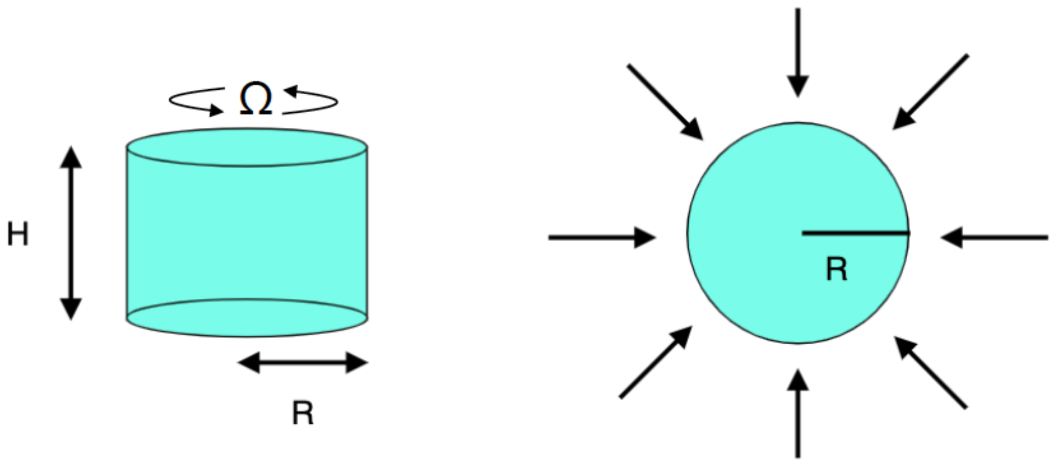
A rotating cylindrical domain of height $H=0.022$ m and radius $R=0.017$ m filled with a solvent is considered, where $\mathsf{\Omega }$ is the rotation rate at which the cylinder rotates around its axis (Figure 1). The dimensions considered are those usually used in experimental studies [14]. The sample is irradiated with microwaves at a frequency of 2.45 GHz, and a power of 80 W. The electromagnetic radiation is normal to the lateral wall. This configuration reproduces the microwave heating in a Discover CEM microwave reactor with a cylindrical cavity [14]. The upper surface is considered to be isolated. This condition is achieved in the laboratory by locating a Teflon piece at the top to avoid the loss of heat through that boundary.

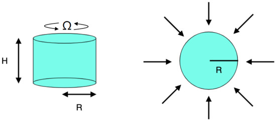
Figure 1. Numerical setup.

The system is governed by the equations

$${\rho }_0{C}_p{\displaystyle \frac{\partial T}{\partial t}}+{\rho }_0{C}_p\mathbf{u}·\nabla T=\kappa {\nabla }^{2}T+Q,$$

(1)

$$\nabla ·\mathbf{u}=0,$$

(2)

$${\displaystyle \frac{\partial \mathbf{u}}{\partial t}}+\mathbf{u}·\nabla \mathbf{u}=-\alpha gT{\mathbf{e}}_z-{\displaystyle \frac{1}{{\rho }_0}}\nabla p+\nu {\nabla }^2\mathbf{u}+2\mathbf{u}\times \mathsf{\Omega }{\mathbf{e}}_z,$$

(3)

where the operators are given in cylindrical coordinates $(r,\varphi ,z)$. In the equations, p is the hydrodynamic pressure, $\mathbf{u}$ is the velocity, T is the temperature, and Q is the power dissipated per unit volume. The Oberbeck–Boussinesq approximation has been used, which considers every fluid property as constant except for the density, which varies linearly with temperature in the buoyancy term, i.e., $\rho ={\rho }_0[1-\alpha (T-T_0)]$, where $\alpha$ is the coefficient of volume expansion and ${\rho }_0$ is the density at $T_0$. In the equations, $\kappa$ is the thermal conductivity, $\nu$ is the kinematic viscosity, $C_p$ is the specific heat, ${\mathbf{e}}_z$ is the unit vector in the z direction, g is the gravity constant, and $\mathsf{\Omega }$ is the rotation rate.

The Oberbeck–Boussinesq approximation is an acceptable assumption, taking into account the relatively small variations in the termophysical variables with temperature. Although some quantitative variation can be found compared to using exact governing equations, the Oberbeck–Boussinesq assumption makes the numerical approach tractable. This approach is commonly used in works that combine natural convection and microwave heating [11,12,21].

The power dissipated per unit volume is given by

$$Q=2\pi f{ϵ}_0{ϵ}^{″}E{E}^{*},$$

(4)

where f is the frequency, ${ϵ}_0$ the permittivity of free space, ${ϵ}^{″}$ the dielectric loss factor, E the electrical field, and $E^{*}$ its complex conjugate. The electrical field is obtained from the simplified equation

$${\displaystyle \frac{{\partial }^{2}E}{\partial r^2}}+{\displaystyle \frac{1}{r}}{\displaystyle \frac{\partial E}{\partial r}}+k_1^{2}E=0$$

(5)

as the microwave incident rays are propagated in the radial direction. In Equation (5), $k_1$ is the wave number, which is defined as $k_1^2={\omega }^2{\mu }_0{ϵ}_0({ϵ}^{\prime }+i{ϵ}^{″})$, with $\omega =2\pi f$, ${ϵ}_0$ the permittivity of free space, ${ϵ}^{\prime }$ the dielectric constant, ${ϵ}^{″}$ the dielectric loss factor and ${\mu }_0$ the free-space permeability. If $E=v+iw$ and $E_0$ is the intensity of the incident field, Equation (5) can be expressed as follows:

$${\displaystyle \frac{{\partial }^{2}v}{\partial r^2}}+{\displaystyle \frac{1}{r}}{\displaystyle \frac{\partial v}{\partial r}}+\psi v-\xi w=0,$$

(6)

$${\displaystyle \frac{{\partial }^{2}w}{\partial r^2}}+{\displaystyle \frac{1}{r}}{\displaystyle \frac{\partial w}{\partial r}}+\psi w+\xi v=0,$$

(7)

where $\psi ={\omega }^2{\mu }_0{ϵ}_0{ϵ}^{\prime }$, $\xi ={\omega }^2{\mu }_0{ϵ}_0{ϵ}^{″}$.

At $r=0$, the boundary conditions are

$${\displaystyle \frac{\partial v}{\partial r}}={\displaystyle \frac{\partial w}{\partial r}}=0$$

(8)

and at $r=R$ [22]:

$$R{\displaystyle \frac{\partial v}{\partial r}}+c_{1}v+c_{2}w=E_0{c}_3,$$

(9)

$$R{\displaystyle \frac{\partial w}{\partial r}}+c_{1}w-c_{2}v=E_0{c}_4,$$

(10)

where

$$\begin{array}{ccc}& & c_1=R{\alpha }_0\left[{\displaystyle \frac{J_1\left({\alpha }_{0}R\right)J_0\left({\alpha }_{0}R\right)+Y_1\left({\alpha }_{0}R\right)Y_0\left({\alpha }_{0}R\right)}{J_0^2\left({\alpha }_{0}R\right)+Y_0^2\left({\alpha }_{0}R\right)}}\right],\hfill \end{array}$$

(11)

$$\begin{array}{ccc}& & c_2={\displaystyle \frac{2}{\pi \left[J_0^2\left({\alpha }_{0}R\right)+Y_0^2\left({\alpha }_{0}R\right)\right]}},\hfill \end{array}$$

(12)

$$\begin{array}{ccc}& & c_3={\displaystyle \frac{-4}{\pi }}{\displaystyle \frac{Y_0\left({\alpha }_{0}R\right)}{J_0^2\left({\alpha }_{0}R\right)+Y_0^2\left({\alpha }_{0}R\right)}},\hfill \end{array}$$

(13)

$$\begin{array}{ccc}& & c_4={\displaystyle \frac{-4}{\pi }}{\displaystyle \frac{J_0\left({\alpha }_{0}R\right)}{J_0^2\left({\alpha }_{0}R\right)+Y_0^2\left({\alpha }_{0}R\right)}},\hfill \end{array}$$

(14)

where J and Y are Bessel functions. Subscripts 0 and 1 refer, respectively, to Bessel functions of zero-order and first-order, and ${\alpha }_0$ is the free-space wave number.

For T, we impose insulating boundary conditions on the top, bottom, and lateral walls:

$$\begin{array}{ccc}& & {\displaystyle \frac{\partial T}{\partial r}}=0\mathrm{a}\mathrm{t}r=R,{\displaystyle \frac{\partial T}{\partial z}}=0\mathrm{at}z=0\mathrm{and}z=H.\hfill \end{array}$$

(15)

For $\mathbf{u}$, the bottom, top, and lateral walls are rigid:

$$\begin{array}{ccc}& & \mathbf{u}=\mathbf{0}\mathrm{at}r=R,z=0,\mathrm{and}z=H.\hfill \end{array}$$

(16)

As the problem has been solved in a primitive variable formulation, the problem of spurious modes for pressure p arises [23]. We have solved this by using the method proposed in Ref. [24], which requires the following additional boundary conditions: the projection of the momentum Equation (3) at $r=R$ and $z=H$ and the continuity Equation (2) at $z=0$.

2.1. Initial Conditions

We consider the following initial conditions in the experiment:

At $t=0$, the sample is at temperature $T_0$:

$$\begin{array}{ccc}& & T=T_0\mathrm{at}t=0.\hfill \end{array}$$

(17)

We consider $T_0=20$ °C in the simulations. Initially, the liquid is at rest:

$$\begin{array}{ccc}& & \mathbf{u}=\mathbf{0}\mathrm{at}t=0.\hfill \end{array}$$

(18)

For pressure,

$$\begin{array}{ccc}& & p=p_0\left(z\right)\mathrm{at}t=0,\hfill \end{array}$$

(19)

where $p_0$ is the initial pressure obtained from Equation (3) with $T=T_0$ and $\mathbf{u}=\mathbf{0}$.

2.2. Numerical Implementation

2.2.1. Temporal Discretization and Projection Scheme

The numerical implementation is a 3D extension, including rotation, of the 2D spectral numerical model on radial microwave irradiation that we developed and validated experimentally in [14].

The governing Equations (1)–(3), boundary conditions (15) and (16), and initial conditions (17)–(19) have been solved numerically by using a second-order time-splitting method [14,25]:

$${\displaystyle \frac{3T^{n+1}-4T^n+T^{n-1}}{2\Delta t}}=-2{\mathbf{u}}^n·\nabla T^n+{\mathbf{u}}^{n-1}·\nabla T^{n-1}+{\displaystyle \frac{k}{{\rho }_0{C}_p}}{\nabla }^2{T}^{n+1}+{\displaystyle \frac{1}{{\rho }_0{C}_p}}{Q}^n$$

(20)

$$\nabla ·{\mathbf{u}}^{n+1}=0$$

(21)

$$\begin{array}{c}\hfill {\displaystyle \frac{3{\mathbf{u}}^{n+1}-4{\mathbf{u}}^n+{\mathbf{u}}^{n-1}}{2\Delta t}}=-2{\mathbf{u}}^n·\nabla {\mathbf{u}}^n+{\mathbf{u}}^{n-1}·\nabla {\mathbf{u}}^{n-1}-{\displaystyle \frac{1}{{\rho }_0}}\nabla p^{n+1}-\alpha g{T}^{n+1}{\mathbf{e}}_{\mathbf{z}}+\\ \hfill \nu {\nabla }^2{\mathbf{u}}^{n+1}+2(2{\mathbf{u}}^n\times \mathsf{\Omega }{\mathbf{e}}_z)-2{\mathbf{u}}^{n-1}\times \mathsf{\Omega }{\mathbf{e}}_z\end{array}$$

(22)

where n is the index for time.

The method consists of the following fractional steps:

• $T^{n+1}$ is obtained from Equation (20). Previously, $Q^n$ is calculated from Equation (4), with $E^n$ being obtained from Equations (6)–(10) by using the dielectric constant ${ϵ}^{\prime }\left(T^n\right)$ and the dielectric loss factor ${ϵ}^{″}\left(T^n\right)$.
• If we apply ∇ to Equation (22) and use Equation (21), a preliminary pressure $\overline{p}$ is calculated.
• A predictor velocity field ${\mathbf{u}}^{*}$ is obtained from Equation (22) by including the predictor pressure $\overline{p}$.
• In a final step, the system

  $${\displaystyle \frac{3}{2\Delta t}}\left({\mathbf{u}}^{n+1}-{\mathbf{u}}^{*}\right)=-{\displaystyle \frac{1}{{\rho }_0}}\nabla \left(p^{n+1}-{\overline{p}}^{n+1}\right),$$

  (23)

  $$\nabla ·{\mathbf{u}}^{n+1}=0,$$

  (24)

  is solved to obtain ${\mathbf{u}}^{n+1}$ and $p^{n+1}$.
  Equation (23) is derived as the subtraction of Equation (22) and Equation (22) with ${\mathbf{u}}^{*}$ and ${\overline{p}}^{n+1}$.

In our computations, a dimensional time step $\Delta t=0.001$ s is used. The time step was chosen to be within the range of convergence of the method. In Ref. [14], where we describe the method for the non-rotational case, we performed a study on the influence of the time step, showing that there is no significant sensitivity to the time step considered within the range in which the method converges (the time step has to be lower than or equal to 0.01 for convergence). The relative differences between simulations with $\Delta t=0.01$ s and $\Delta t=0.001$ s were of the order ${10}^{-3}$.

2.2.2. Spatial Discretization

For the spatial discretization we use a pseudo-spectral method, with Chebyshev collocation in the coordinates r and z and a Fourier expansion in the coordinate $\varphi$. Each field is expanded as

$$x(r,\varphi ,z)=\sum _{k=-K/2}^{K/2-1}{F}_k(r,z)e^{ik\varphi },$$

(25)

with $F_0(r,z)$ and $F_{-K/2}(r,z)$ being real and $F_{-k}(r,z)={\overline{F}}_k(r,z)$ for $k=1:K/2-1$, where ${\overline{F}}_k$ is the complex conjugate of $F_k$.

We expand the coefficients $F_k$ in Chebyshev polynomials:

$$F_k(r,z)=\sum _{l=0}^L\sum _{m=0}^M{f}_{lm}{T}_l\left(r\right)T_m\left(z\right).$$

(26)

where $T_m$ is the m-th Chebyshev polynomial. Evaluations are performed at the Gauss–Lobatto collocation points: $r_j=\mathsf{\Gamma }cos{\displaystyle \frac{\pi j}{L}}$ for $j=0:L$; $z_j=\mathsf{\Gamma }cos{\displaystyle \frac{\pi j}{M}}$ for $j=0:M$ [14,23]. This requires a transformation, changing domain $\mathcal{D}$ to $[-1,1]\times [-1,1]\times [0,2\pi ]$ due to implementation based on Chebyshev collocation. In our calculations, $L=41$, $M=41$, and $K=32$ are considered.

The use of spectral methods permits the achievement of accurate solutions with low-order spatial expansions compared to other methods, which reinforces the importance of the numerical method we have developed. A limitation of the method is the presence of ill-conditioned matrices that restricts the range of permitted order expansions. Another limitation is the type of domain in which they can be used: only squares or cuboids (or domains reducible to them) are permitted; other domains require domain decomposition techniques to be dealt with.

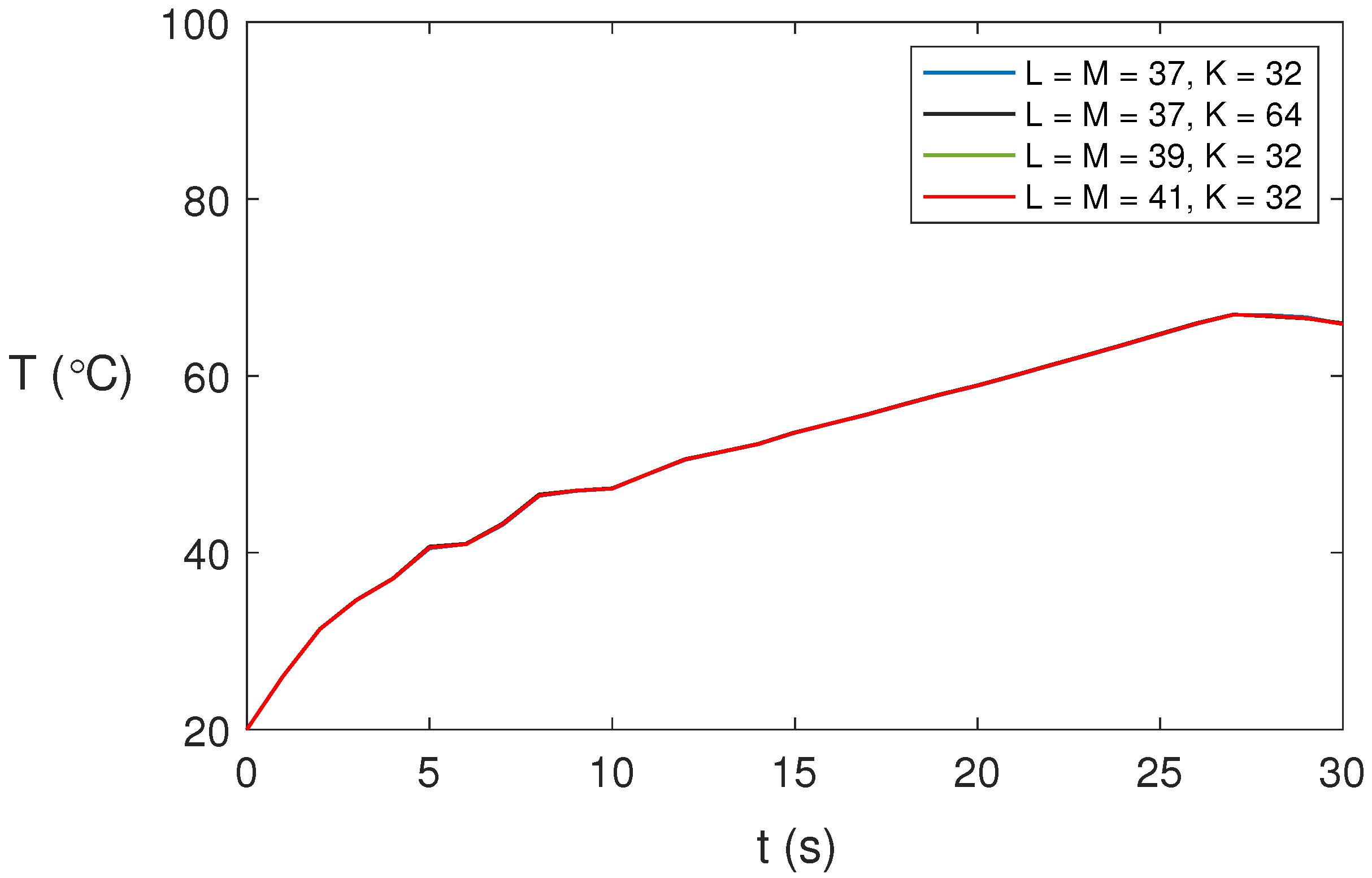
We studied the dependence of the solution on the spatial expansions. Figure 2 shows the temperature profiles at point $P_1(0.0004,0,0.02)$ for different spatial expansions and $\Delta t=0.001$ s for water at $2.45$ GHz, 80 W, and $\mathsf{\Omega }={\displaystyle \frac{\pi }{60}}$. As shown, there is no significant influence of the spatial expansion on the numerical results obtained. We have considered $L=41$, $M=41$, and $K=32$ in our computations to ensure accurate solutions for the non-axisymmetric cases.

Figure 2. Predicted temperature profiles for water at $2.45$ GHz, 80 W, and $\mathsf{\Omega }={\displaystyle \frac{\pi }{60}}$ at point $P_1(0.0004,0,0.02)$ for different spatial expansions and time step $\Delta t=0.001$ s.

Using a time step $\Delta t=0.001$ s and $L=41$, $M=41$, and $K=32$ the CPU time on a 3.6 GHz Intel Core i9 128 GB is $10.32$ s for each iteration. The code implementation was performed using the software MATLAB R2024b.

3. Results and Discussion

In this section, we report results on the effect of rotation on the heating process for two different solvents subject to microwave heating: water and ethylene glycol. Table 1 summarizes the dielectric properties and other parameters used for the study.

Table 1. Input parameters for the solvents used for computations [26,27,28,29].

Parameter	Water	Ethylene Glycol
$\mathrm{Density} \mathrm{at} T_0,{\rho }_0$ (kg m−3)	993	1112
$\mathrm{Conductivity},k$ (W m−1 °C−1)	$0.63$	$0.25$
$\mathrm{Specific} \mathrm{heat},C_p$ (J kg−1 °C−1)	4179	2408
$\mathrm{Kinematic} \mathrm{viscosity},\nu$ (m2 s−1)	$6.5\times {10}^{-7}$	$1.78\times {10}^{-5}$
$\mathrm{Volumetric} \mathrm{expansion} \mathrm{coefficient},\alpha$ (°C−1)	$2.14\times {10}^{-4}$	$5.7\times {10}^{-4}$
$\mathrm{Initial} \mathrm{temperature},T_0$ (°C)	20	20
$\mathrm{Frequency},f$ (GHz)	$2.45$	$2.45$
$\mathrm{Power},P$ (W)	80	80
$\mathrm{Rotation} \mathrm{rate},\mathsf{\Omega }$ (s−1)	0 to ${\displaystyle \frac{\pi }{60}}$	0 to ${\displaystyle \frac{\pi }{30}}$
$\mathrm{Dielectric} \mathrm{constant},{ϵ}^{\prime }$	$-0.076T+74.36$	$0.001T^2-0.099T+11.46$
$\mathrm{Dielectric} \mathrm{loss} \mathrm{factor},{ϵ}^{″}$	$0.003T^2-0.458T+20.98$	$-0.003T^2+0.262T+8.68$

3.1. State Character Depending on $\mathsf{\Omega }$

The initial state in the experiment is the axisymmetric state, $T_0=20$  °C, and $u=0$ m s⁻¹. The effect of rotation on the character of the developed flow (axisymmetric or non-axisymmetric) during the microwave heating depends on the characteristics of the solvent under study.

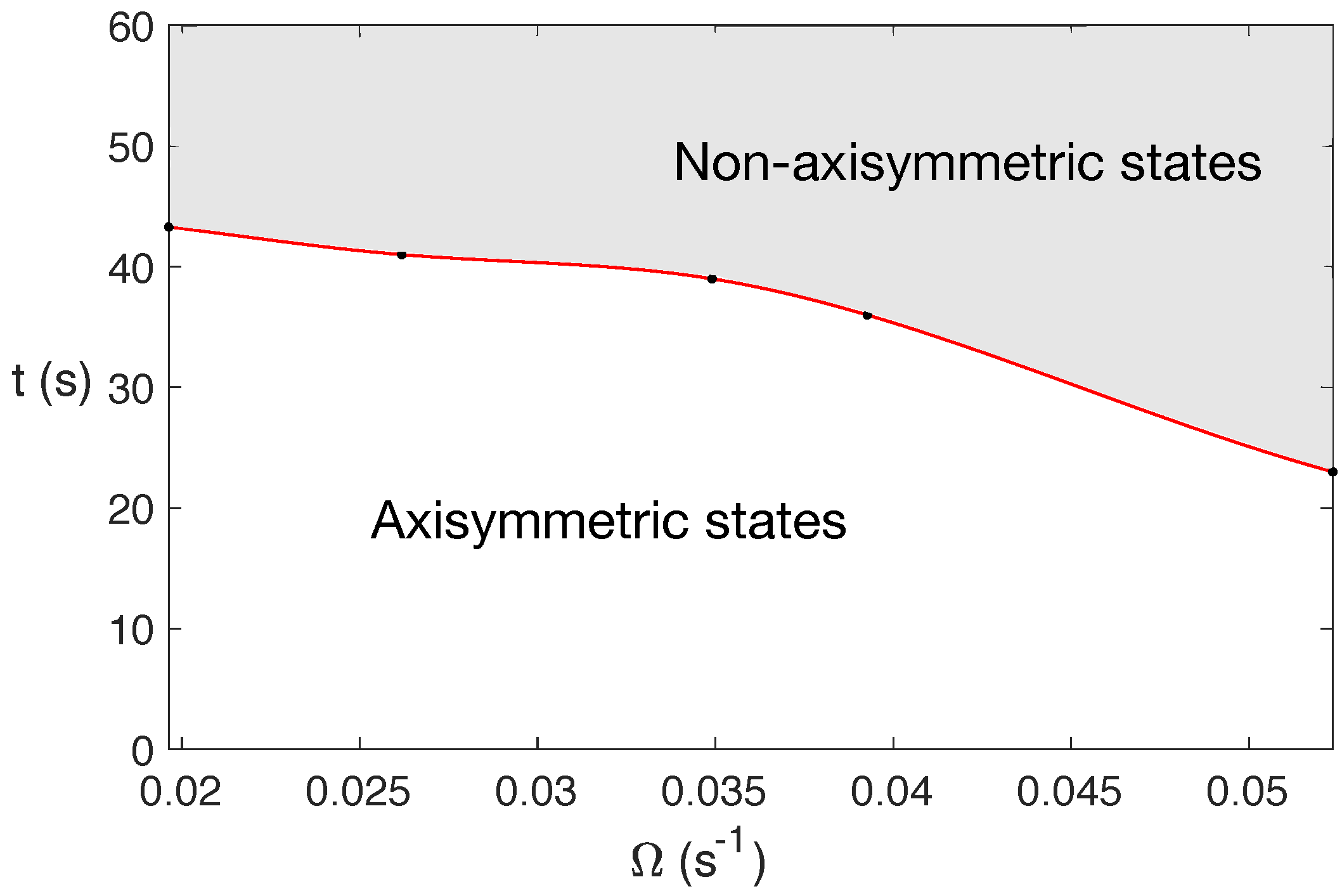
For water under MW at 2.45 GHz and 80 W, the state becomes completely 3D before 60 s, with this change in character occurring earlier in time for larger rotation rates. This is shown in Figure 3, that displays a diagram of the state character depending on the rotation rate $\mathsf{\Omega }$ and t at 2.45 GHz and 80 W.

Figure 3. Diagram of the state character when varying the rotation rate $\mathsf{\Omega }$ and t for water under MW at 2.45 GHz and 80 W. The shaded zone corresponds to the region where fully 3D states are developed.

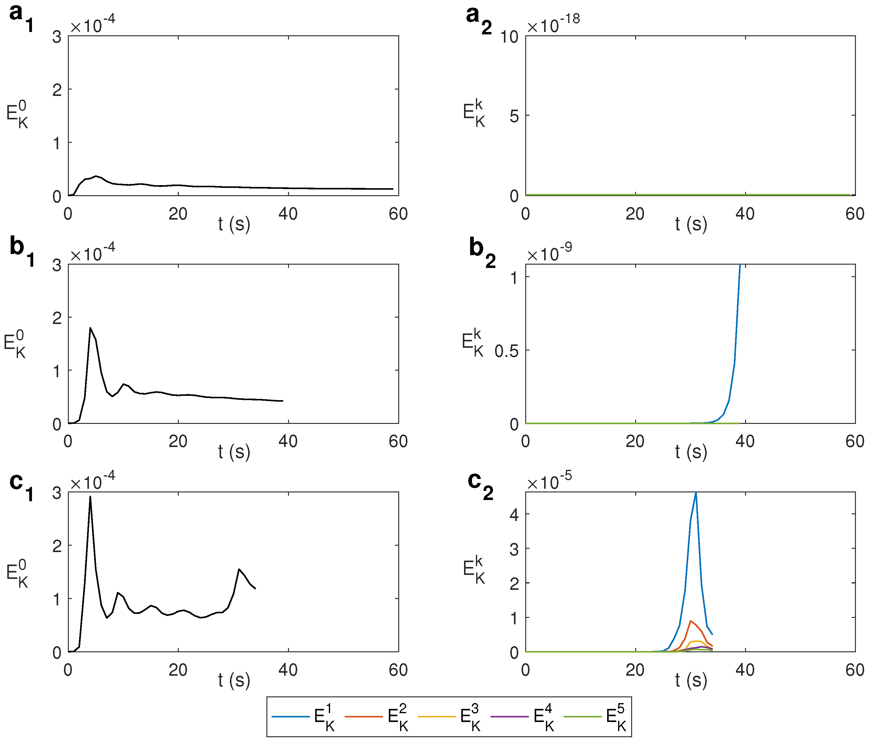
The change from an axisymmetric state to non-axisymmetric can be determined by the spectral decomposition of the kinematic energy $E_K$ with the azimuthal wave number k. The modal kinetic energy $E_K^k$ is computed as $E_K^k={\displaystyle \frac{1}{2}}{\int }_{z=0}^{z=H}{\int }_{r=0}^{r=R}{\mathbf{u}}_k·{\mathbf{u}}_k^{*}rdrdz$, where ${\mathbf{u}}_k$ is the Fourier mode k of the velocity field and ${\mathbf{u}}_k^{*}$ its complex conjugate. Figure 4 shows this spectral decomposition for water under MW at 2.45 GHz and 80 W for different values of $\mathsf{\Omega }$. For $\mathsf{\Omega }=0$ s⁻¹, i.e., without rotation, the state remains axisymmetric during the first 59 s, as displayed in Figure 4a, where only the mode $k=0$ is active. For $\mathsf{\Omega }={\displaystyle \frac{\pi }{80}}$ s⁻¹, displayed in Figure 4b, the energy of the mode $k=1$ begins to grow for $t=35$ s, developing a 3D state from that instant. For larger $\mathsf{\Omega }$, the growth of modes different from 0 occurs earlier in time, as shown in Figure 4c, that displays the case $\mathsf{\Omega }={\displaystyle \frac{\pi }{60}}$ s⁻¹. As observed, around $t=25$ s the energy of the mode $k=1$ begins to grow, as does the energy of other modes. Simulations are stopped when the temperature rises above 100 °C as the model used does not consider changes of state. From the results above it can be asserted that an increase in the rotation rate leads to achieving a fully 3D state earlier.

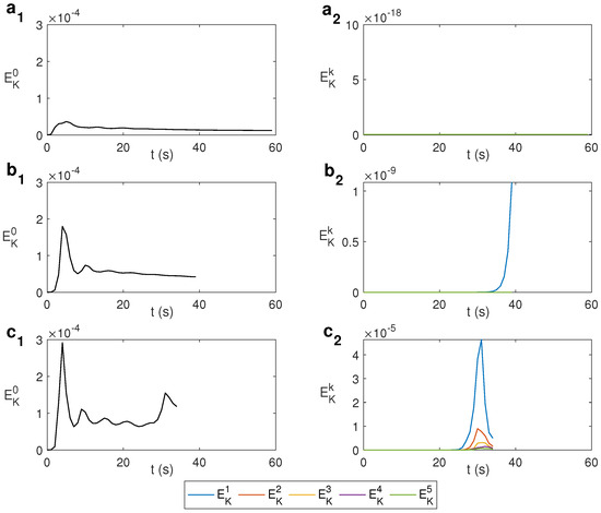
Figure 4. Spectral decomposition of the kinematic energy $E_K$ with the azimuthal wave number k for different values of $\mathsf{\Omega }$ for water under MW at 2.45 GHz and 80 W. (a) $\mathsf{\Omega }=0$ s⁻¹; (b) $\mathsf{\Omega }={\displaystyle \frac{\pi }{80}}$ s⁻¹; (c) $\mathsf{\Omega }={\displaystyle \frac{\pi }{60}}$ s⁻¹.

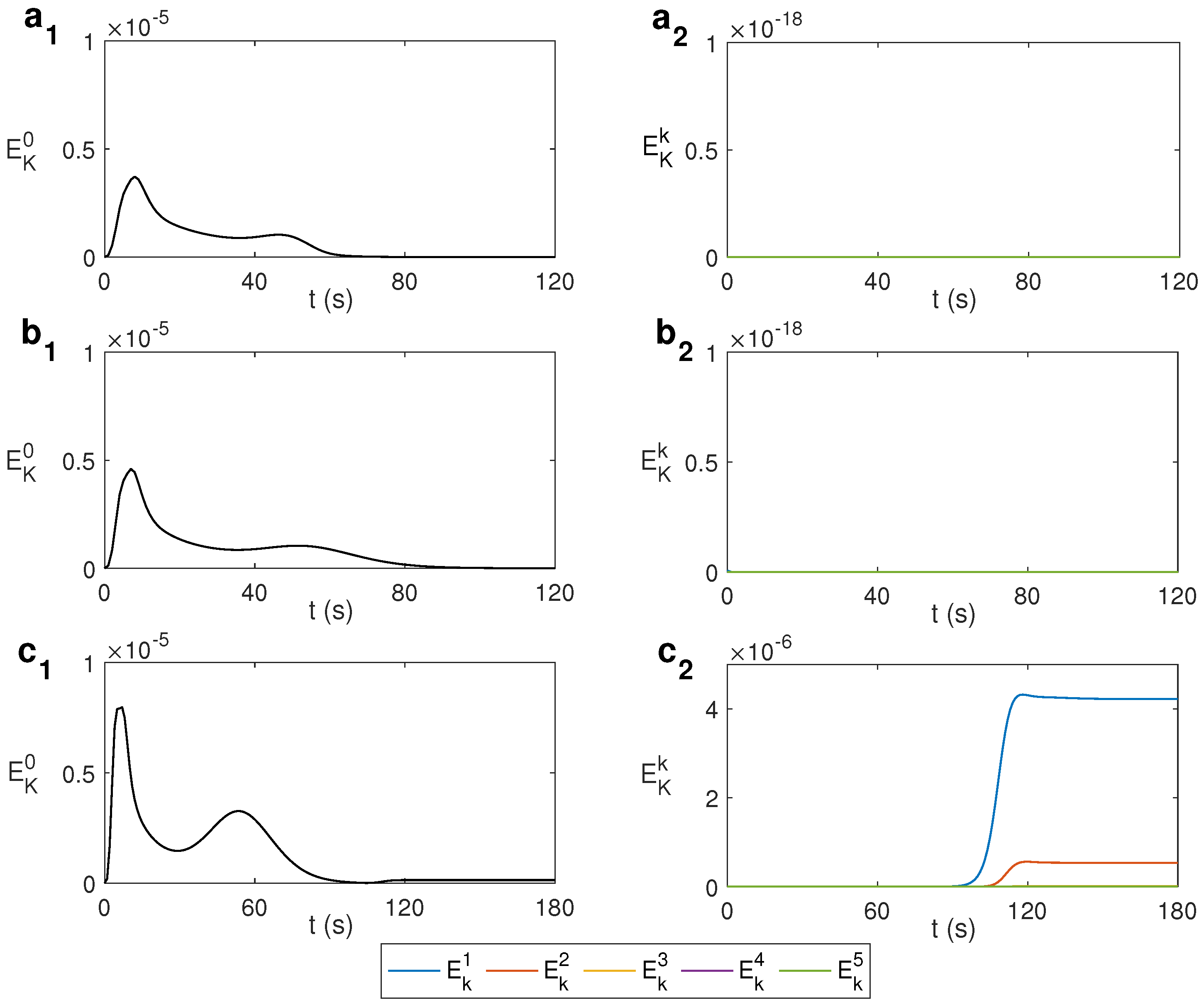
Figure 5 displays the spectral decomposition of the kinematic energy for ethylene glycol under MW at 2.45 GHz and 80 W. As observed in Figure 5b, corresponding to $\mathsf{\Omega }={\displaystyle \frac{\pi }{80}}$ s⁻¹, only the mode $k=0$ is present, i.e., the state remains axisymmetric and similar to the non-rotation case shown in Figure 5a. It is necessary to increase the rotation rate to $\mathsf{\Omega }={\displaystyle \frac{\pi }{30}}$ s⁻¹ to localize a state that becomes fully 3D, which occurs after 90 s of microwave heating, as shown in Figure 5c, where modes $k=1$ and $k=2$ activate.

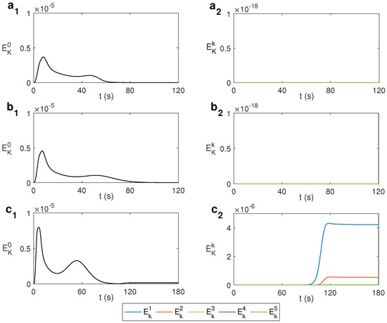
Figure 5. Spectral decomposition of the kinematic energy $E_K$ with the azimuthal wave number k for different values of $\mathsf{\Omega }$ for ethylene glycol under MW at 2.45 GHz and 80 W. (a) $\mathsf{\Omega }=0$ s⁻¹; (b) $\mathsf{\Omega }={\displaystyle \frac{\pi }{80}}$ s⁻¹; (c) $\mathsf{\Omega }={\displaystyle \frac{\pi }{30}}$ s⁻¹.

3.2. Effect of Rotation on the Velocity Flow and Temperature Profile

3.2.1. Solvent 1: Water

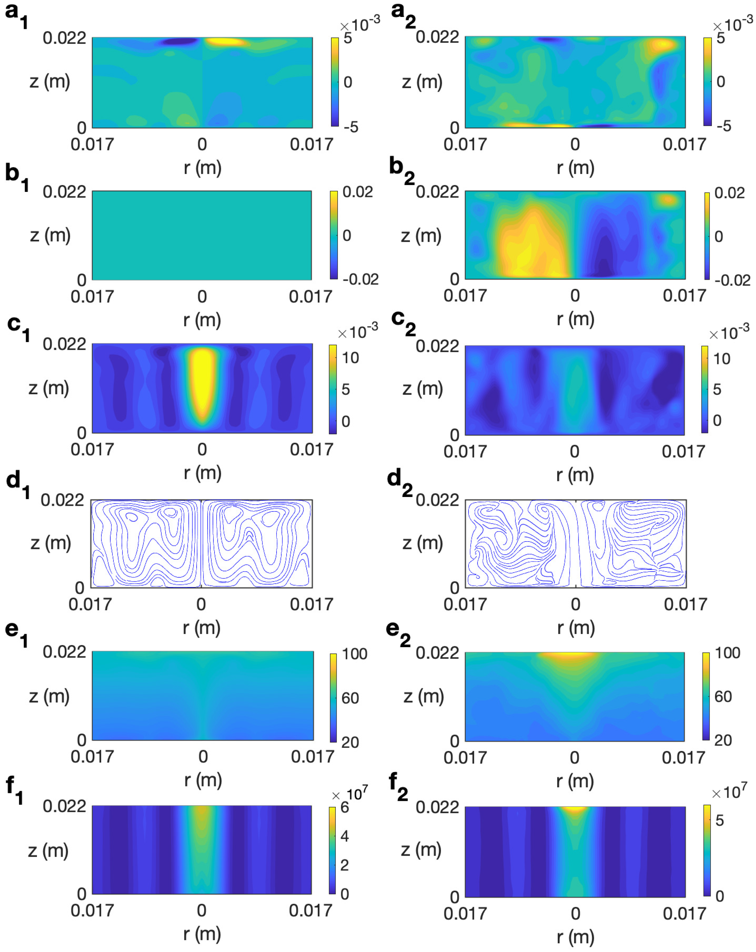
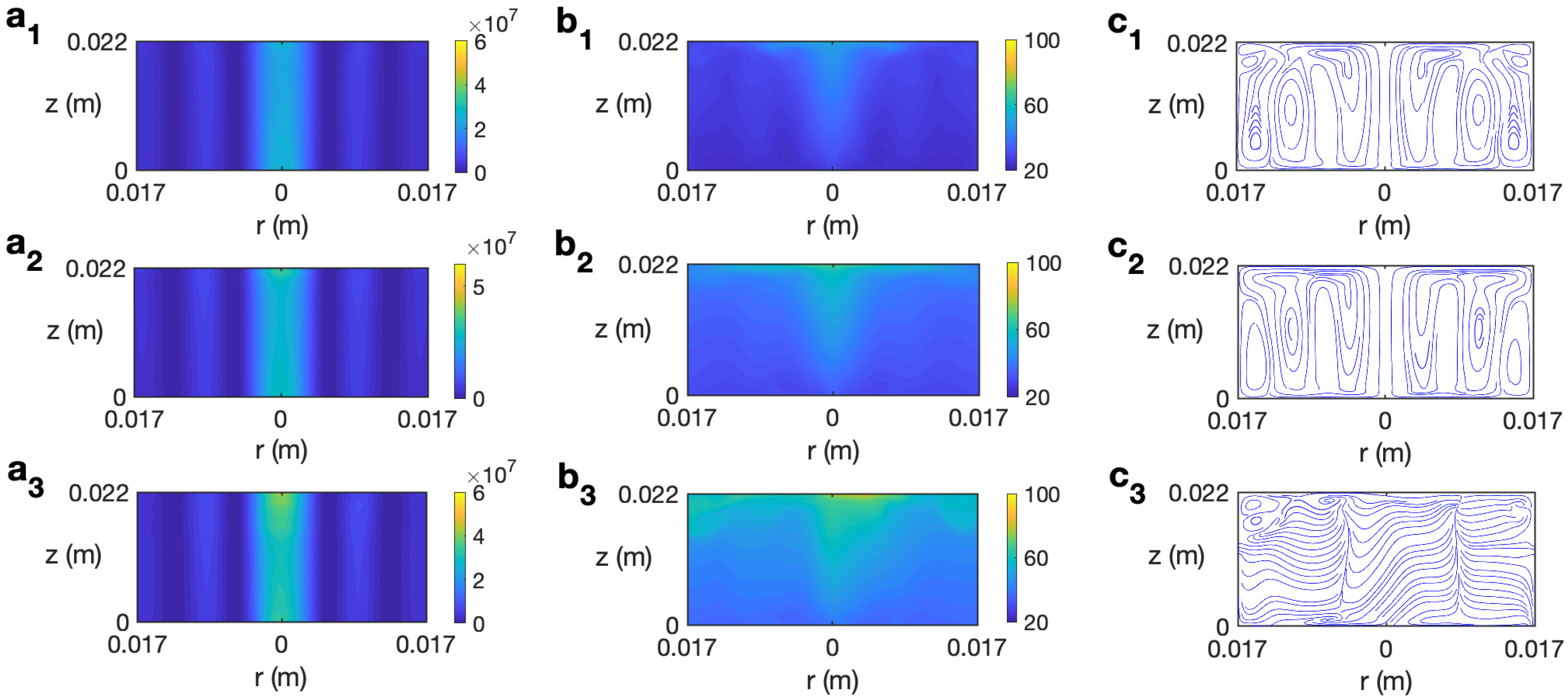
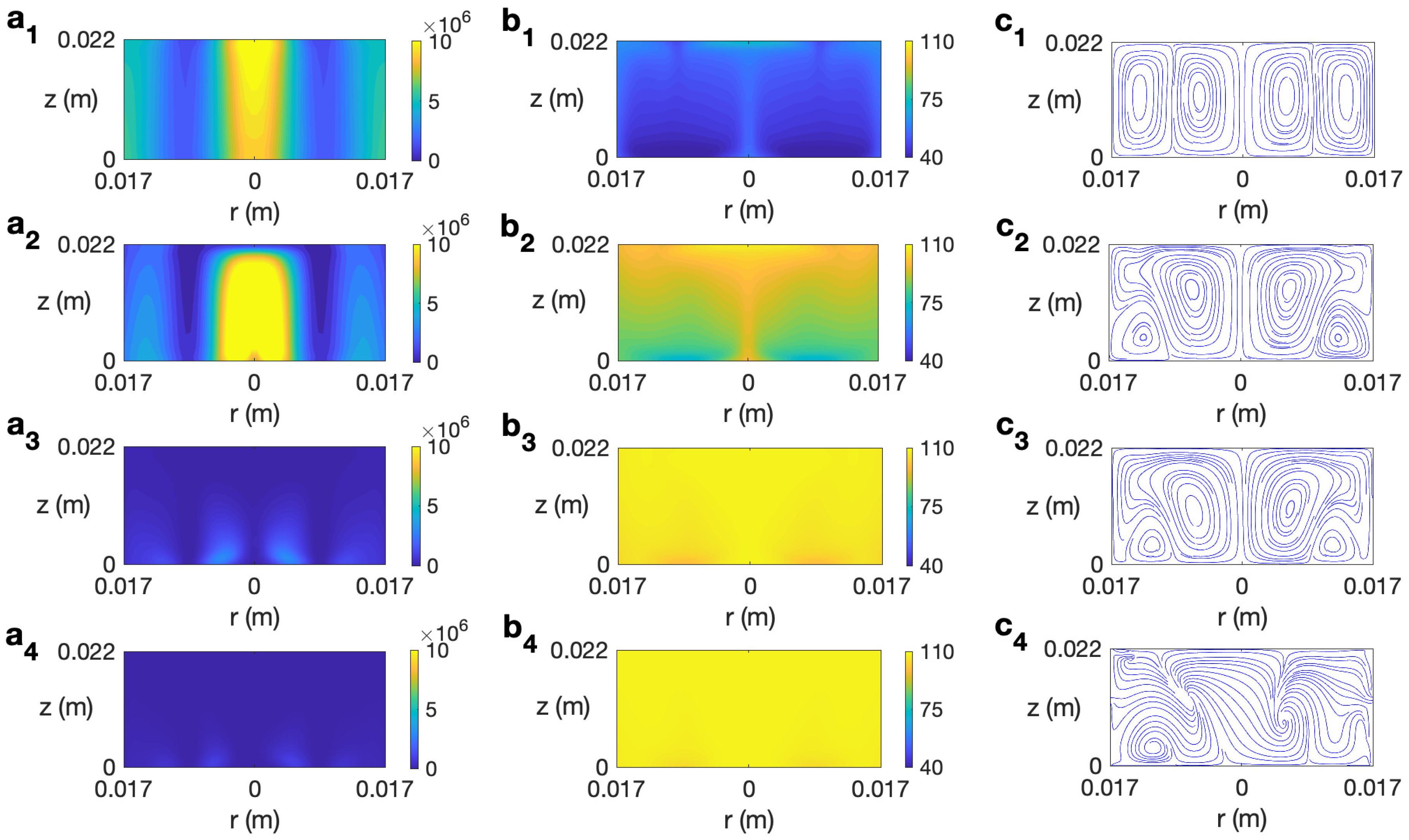
We start studying the behavior of a sample of water. In Refs. [14,30], the behavior of this liquid under microwave heating without rotating the sample is detailed. Figure 6 (left column) shows the simulated solutions at $\varphi =0$ $(\varphi =\pi )$ for $t=34$ s for the case without rotation at 2.45 GHz and 80 W. As observed, the state remains axisymmetric, with no azimuthal velocity (Figure 6 (b₁)). The profile of temperature shows a stronger heating along the axis of the cylinder (Figure 6 (e₁)) that is mainly determined by the microwave power absorption Q (Figure 6 (f₁)), that presents a higher intensity in that central part. Note that this is not a general feature and it depends on the liquid considered and the dimensions of the sample, as shown in Ref. [31]. Heat is also distributed along the upper levels due to convection provided by the radial velocity (Figure 6 (a₁)).

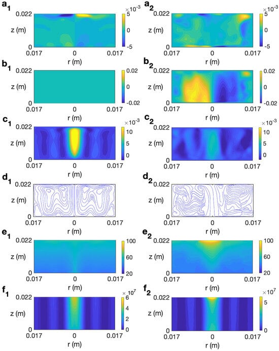
Figure 6. Contours of the predicted velocity, temperature, and microwave power absorption Q for water for MW at 2.45 GHz and 80 W at $\varphi =0$ $(\varphi =\pi )$ for $t=34$ s. (a₁–f₁) $\mathsf{\Omega }=0$ s⁻¹; (a₂–f₂) $\mathsf{\Omega }={\displaystyle \frac{\pi }{60}}$ s⁻¹. From top to bottom: $u_r$, $u_{\varphi }$, $u_z$, streamlines, T, and Q.

There is an intense vertical upward movement along the cylindrical axis (Figure 6 (c₁)). At upper levels there is movement from the center of the cylinder to the outer part, as shown in Figure 6 (a₁). The combined effect of the radial and vertical velocity components is described through the velocity field and streamlines displayed in Figure 6 (d₁), that shows the strong upward motion along the axis and the outward motion at the top levels.

When rotation is included in the system, significant differences are appreciated. As shown in Section 3.1, the inclusion of rotation makes the state become fully 3D earlier in time. For $\mathsf{\Omega }={\displaystyle \frac{\pi }{60}}$ s⁻¹ it occurs around 25 s. Figure 7 shows the temporal evolution of the temperature, velocity field, and microwave power absorption for water at 2.45 GHz and 80 W, $\mathsf{\Omega }={\displaystyle \frac{\pi }{60}}$ s⁻¹ for $t=10$ s, $t=20$ s, and $t=30$ s. While the state remains axisymmetric (for $t<25$ s), there is stronger heating along the cylinder’s axis, related to a higher intensity of the Q profile in that part and fluid motion upwards along the central axis. This can be appreciated in Figure 7 (a₁–c₁, a₂–c₂) for times $t=10$ s and $t=20$ s, respectively. The loss of axisymmetry complicates the fluid motion, breaking the stable movement of the fluid at the central part of the domain, as depicted in Figure 7 (a₃–c₃). As a consequence, the localization of heat along the axis of the cylinder reduces, keeping the heat located at the upper central part.

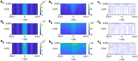
Figure 7. Contours of the predicted microwave power absorption Q, temperature, and velocity field and streamlines for water for MW at 2.45 GHz and 80 W at $\varphi =0$ $(\varphi =\pi )$ for $\mathsf{\Omega }={\displaystyle \frac{\pi }{60}}$ s⁻¹. (a₁–c₁) $t=10$ s; (a₂–c₂) $t=20$ s; (a₃–c₃) $t=30$ s. From left to right: Q, temperature, and streamlines.

Figure 6 (right column) shows the profiles for velocity, temperature, and microwave power absorption at $\varphi =0$ $(\varphi =\pi )$, $\mathsf{\Omega }=60$ s⁻¹, and $t=34$ s. The time $t=34$ s is the final time considered in the simulation because beyond this time the water temperature goes above 100 °C and the model used is not valid as it does not consider changes of state. The rotation included in the system gives place to an azimuthal movement, as shown in Figure 6 (b₂). This implies a clockwise motion of the fluid in the azimuthal direction. It is noted that the vertical velocity component has smaller values along the cylinder axis (Figure 6 (c₂)) than in the non-rotation case; therefore, the upward motion is reduced in that zone. The temperature shows a stratified profile but, differently to what was observed for the case without rotation, the hotter region is localized in the central upper part of the cell (Figure 6 (e₂)). Note also the concentration of intensity in that part for the microwave power absorption (Figure 6 (f₂)). These fully 3D results agree with simulations in [21] that use an axisymmetric model, and allow us to conclude that, in the case of radial irradiation, rotation does not improve the temperature homogeneity in the sample; on the contrary, an increase in non-uniformity for temperature is reported.

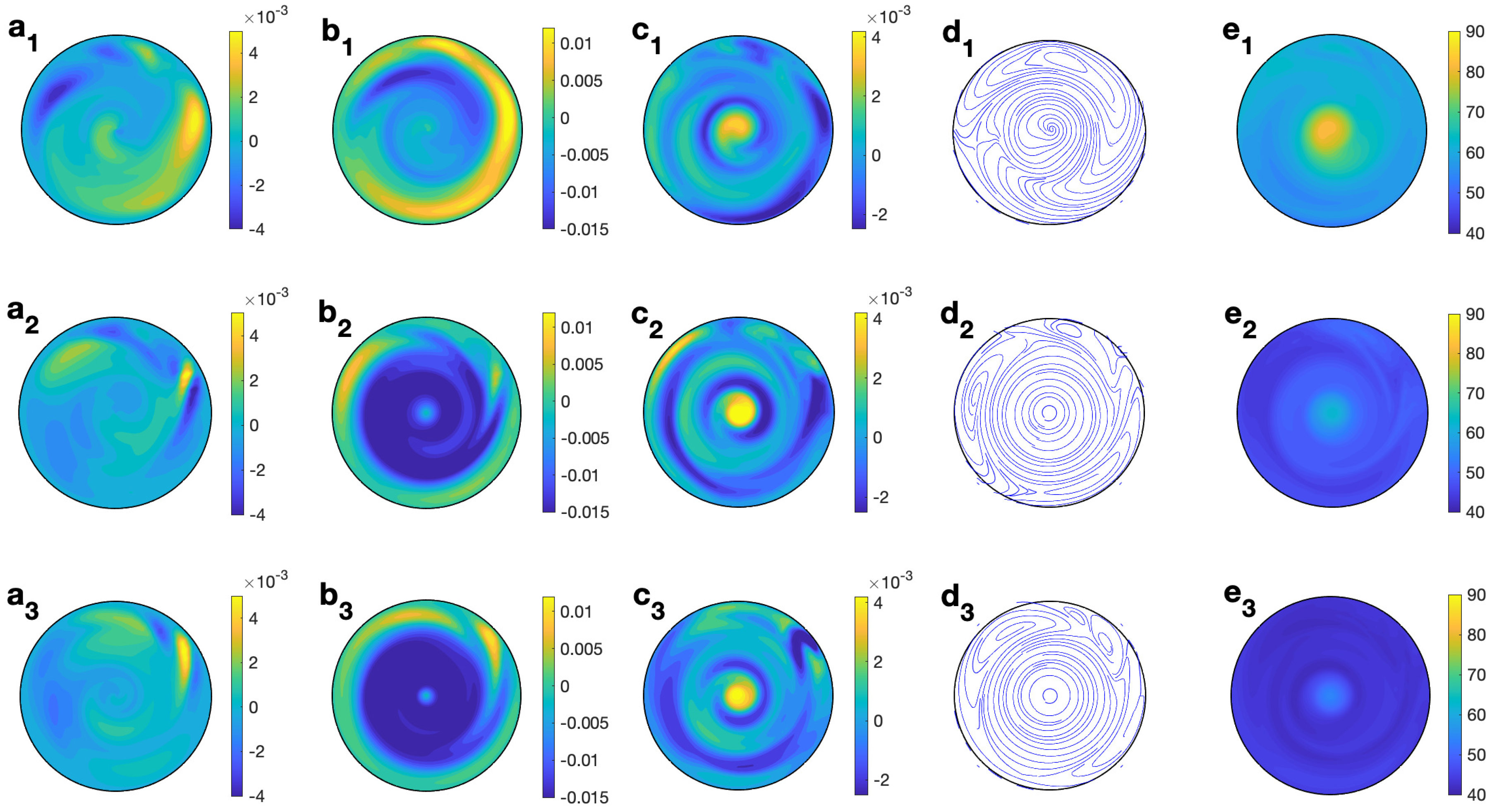
To analyze deeply the three dimensional behavior of the solvent, Figure 8 shows the profiles of temperature and velocity for water for MW at 2.45 GHz and 80 W at different values of z for $t=34$ s and $\mathsf{\Omega }={\displaystyle \frac{\pi }{60}}$ s⁻¹. The non-axisymmetric character of the flow is clearly observed from any profile. It is notable that the magnitude and profile of $u_{\varphi }$ (Figure 8 (b₁–b₃)), mainly at medium and lower levels, when combined with the radial velocity component (small and concentrated in the outer part, as depicted in Figure 8 (a₁–a₃), it changes to the velocity field shown in Figure 8 (d₁–d₃), where a clear clockwise rotation is reported. $u_z$ profiles (Figure 8 (c₁–c₃)), show upward motion all along the cylinder’s axis. The temperature profile with height (Figure 8 (e₁–e₃)) shows a hotter central region in the cell, especially at the upper levels.

Figure 8. Contour of the predicted velocity and temperature for water for MW at 2.45 GHz and 80 W at different values of z for $t=34$ s and $\mathsf{\Omega }={\displaystyle \frac{\pi }{60}}$ s⁻¹. (a₁–e₁) $z=0.02$ m; (a₂–e₂) $z=0.0105$ m; (a₃–e₃) $z=0.005$ m. From left to right: $u_r$, $u_{\varphi }$, $u_z$, streamlines, and T.

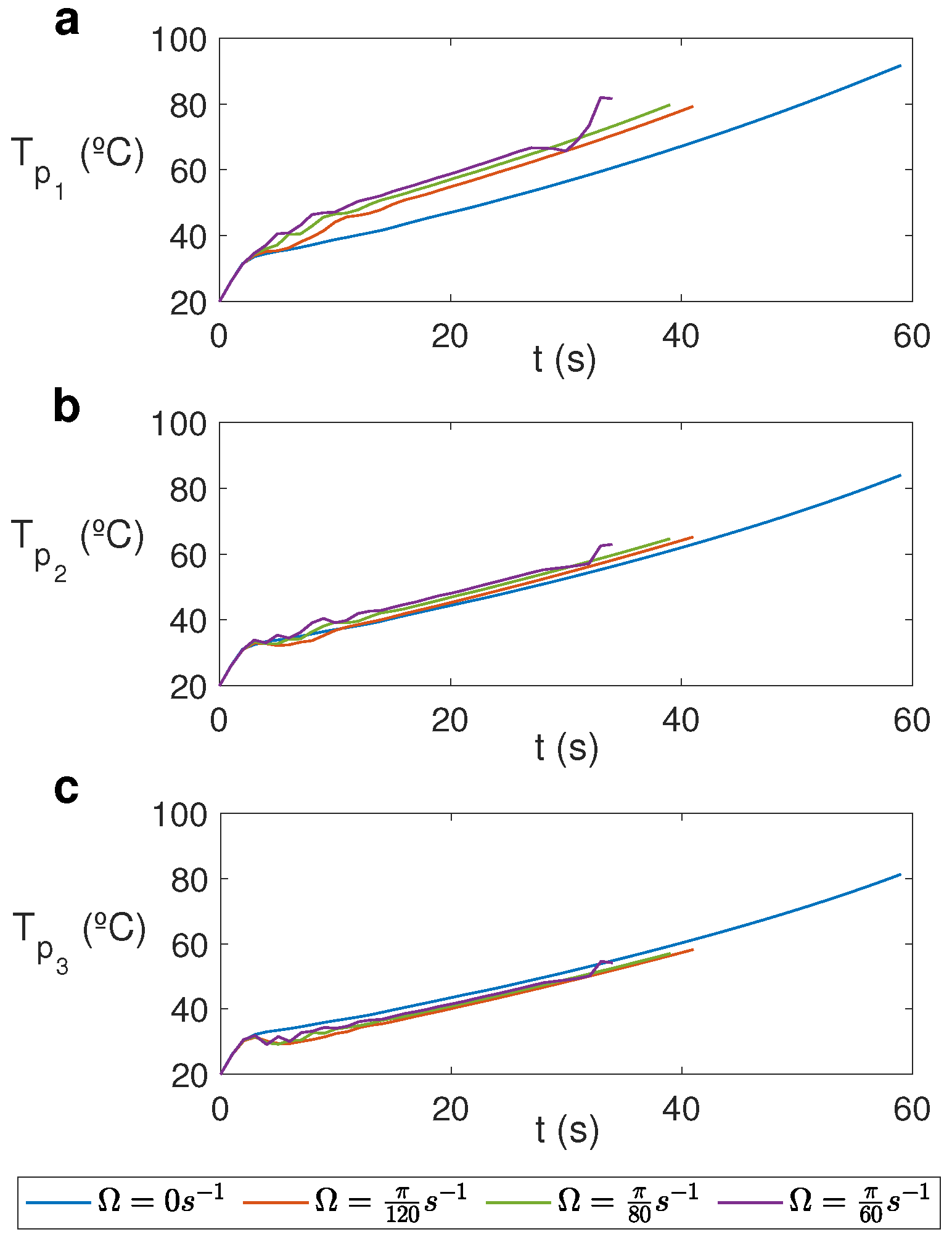
Figure 9 displays the temporal evolution of temperature at three different points at a distance of $0.0004$ m from the cylinder’s axis, $\varphi =0$, and different heights for different rotation rates. Significant variations are registered at the upper levels (Figure 9a), where temperature is higher in the rotation cases and it increases for greater rotation rates. Each line ends at the time at which 100 °C is registered in the cell and therefore the model cannot be used.

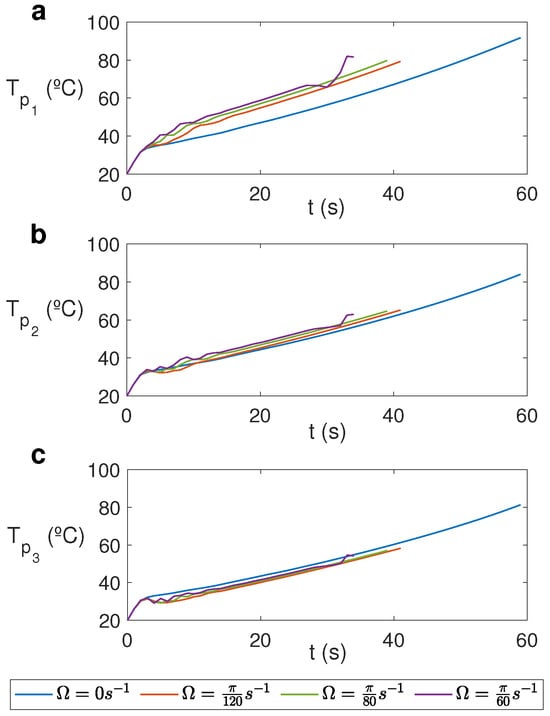
Figure 9. Temporal evolution of temperature at three different points for water for MW at 2.45 GHz and 80 W at different values of $\mathsf{\Omega }$. (a) $P_1(0.0004,0,0.02)$; (b) $P_2(0.00004,0,0.0105)$; (c) $P_3(0.0004,0,0.005)$.

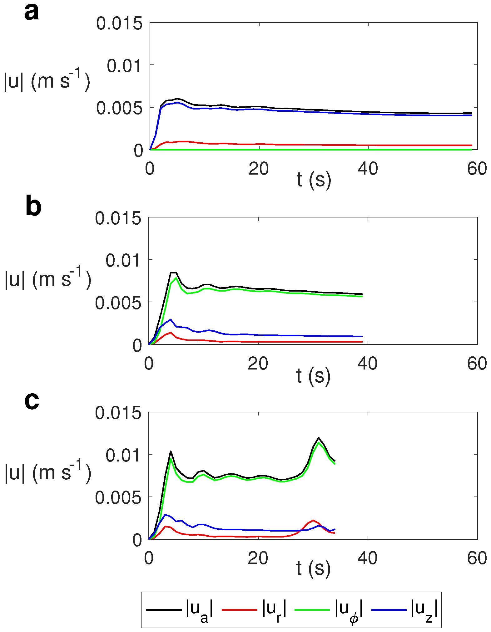
The evolution of the average velocity $|{\mathbf{u}}_a|$ and the average radial ($|{\mathbf{u}}_r|$), azimuthal ($|{\mathbf{u}}_{\varphi }|$), and vertical ($|{\mathbf{u}}_z|$) velocities for different values of the rotation rate is depicted in Figure 10. We calculated the average velocity $|{\mathbf{u}}_a|$ as

$$|{\mathbf{u}}_a|={\displaystyle \frac{\int \int {\int }_{D}r\left|\mathbf{u}(r,\varphi ,z)\right|drd\varphi dz}{Vol\left(D\right)}}$$

(27)

where $\left|\mathbf{u}\right|=\sqrt{u_r^2+u_{\varphi }^2+u_z^2}$. For the computation of $|{\mathbf{u}}_x|$, $x=r,\varphi ,z$, Equation (27) was used with $\left|\mathbf{u}\right|=|u_x|$. We iteratively used the trapezoidal method to compute the integrals.

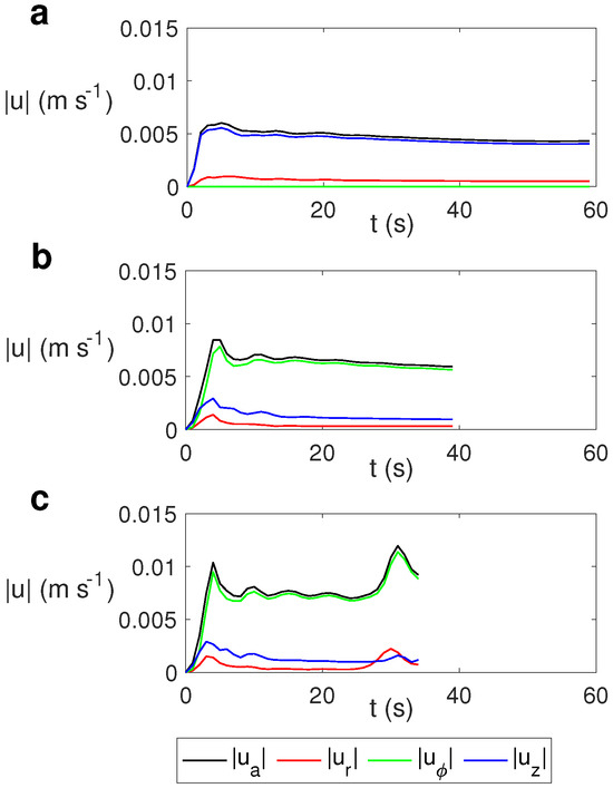
Figure 10. Time evolution of the average velocity $|{\mathbf{u}}_a|$ and the average radial $|{\mathbf{u}}_r|$, azimuthal $|{\mathbf{u}}_{\varphi }|$, and vertical $|{\mathbf{u}}_z|$ velocities for water for MW at 2.45 GHz and 80 W at different values of $\mathsf{\Omega }$. (a) $\mathsf{\Omega }=0$ s⁻¹; (b) $\mathsf{\Omega }={\displaystyle \frac{\pi }{80}}$ s⁻¹; (c) $\mathsf{\Omega }={\displaystyle \frac{\pi }{60}}$ s⁻¹.

As observed, the average velocity for the case without rotation (Figure 10a) is essentially the vertical velocity, while in the cases with rotation it is essentially the azimuthal component (Figure 10b,c). As the rotation rate increases, the average velocity and the azimuthal component increase slightly, with the variation in the average values of the radial and vertical velocity components not being significant for different values of $\mathsf{\Omega }$.

3.2.2. Solvent 2: Ethylene Glycol

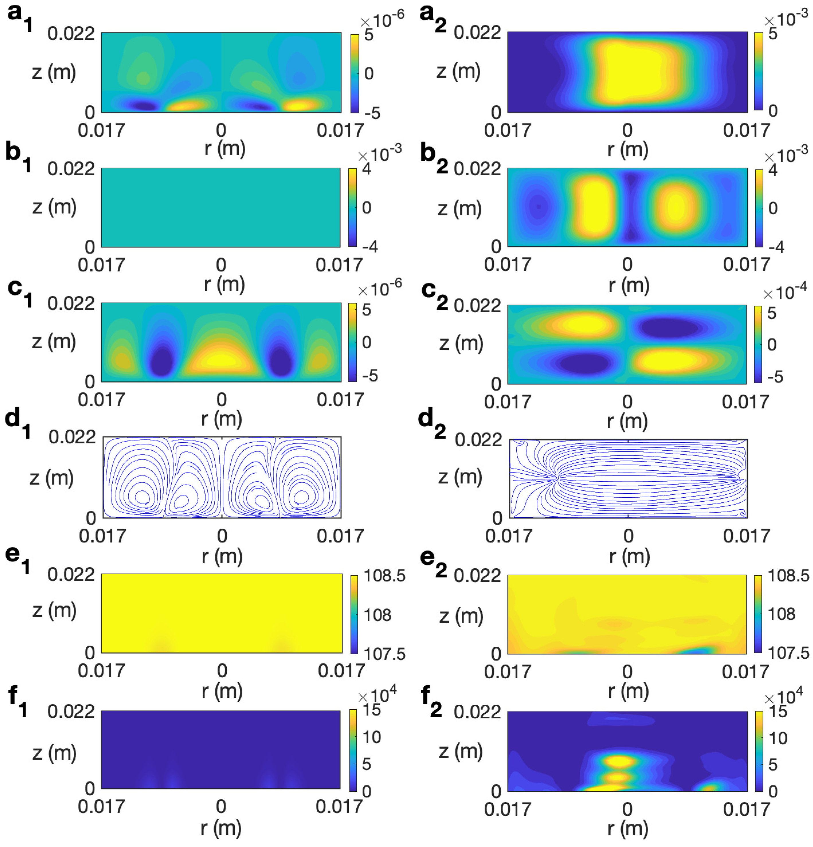
The behavior of ethylene glycol, a solvent more viscous than water and highly susceptible to microwave irradiation [30], is analyzed next. Figure 11 displays the temporal evolution of microwave power absorption, temperature, and velocity field for ethylene glycol at 2.45 GHz and 80 W for $\mathsf{\Omega }={\displaystyle \frac{\pi }{30}}$ s⁻¹. The profiles reported for $t<90$ s are very similar to the state found for the non-rotation case [30] or other rotation rates lower than ${\displaystyle \frac{\pi }{30}}$. Figure 11 (a₁–c₁) shows the state for $t=20$ s. The dielectric characteristics of the solvent imply the highest values of Q are at the center of the cylinder and at the lateral wall (Figure 11 (a₁)). The corresponding profiles of temperature and velocity are displayed in Figure 11 (b₁ and c₁). Two convective rolls are formed, one raising the hot fluid along the cylinder’s axis towards the top layer and the other one along the lateral wall. This implies a height-stratified profile for temperature. Higher temperatures are found at the center of the vessel and at upper levels. For longer times, the inner convective roll expands towards the lateral wall at upper levels (Figure 11 (c₂)), moving hot fluid to those zones (Figure 11 (b₂)). The dissipation factor for ethylene glycol strongly decays for higher temperatures [30]. This explains the profile of Q for $t=80$ s, shown in Figure 11 (a₃). The cell is almost at a homogeneous temperature around 108 °C (Figure 11 (b₃)). Around $t=90$ s, the state becomes fully 3D, as observed in the velocity field depicted in Figure 11 (c₄) for $t=95$ s, but no relevant changes are experienced in the microwave power absorption and temperature profiles (Figure 11 (a₄ and b₄)). The temperature in the cell is practically equal to 108 °C everywhere.

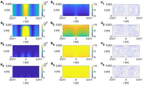
Figure 11. Contours of the predicted microwave power absorption Q, temperature, and velocity field and streamlines for ethylene glycol for MW at 2.45 GHz and 80 W at $\varphi =0$ $(\varphi =\pi )$ for $\mathsf{\Omega }={\displaystyle \frac{\pi }{30}}$ s⁻¹. (a₁–c₁) $t=20$ s; (a₂–c₂) $t=50$ s; (a₃–c₃) $t=80$ s; (a₄–c₄) $t=95$ s. From left to right: Q, temperature, and streamlines.

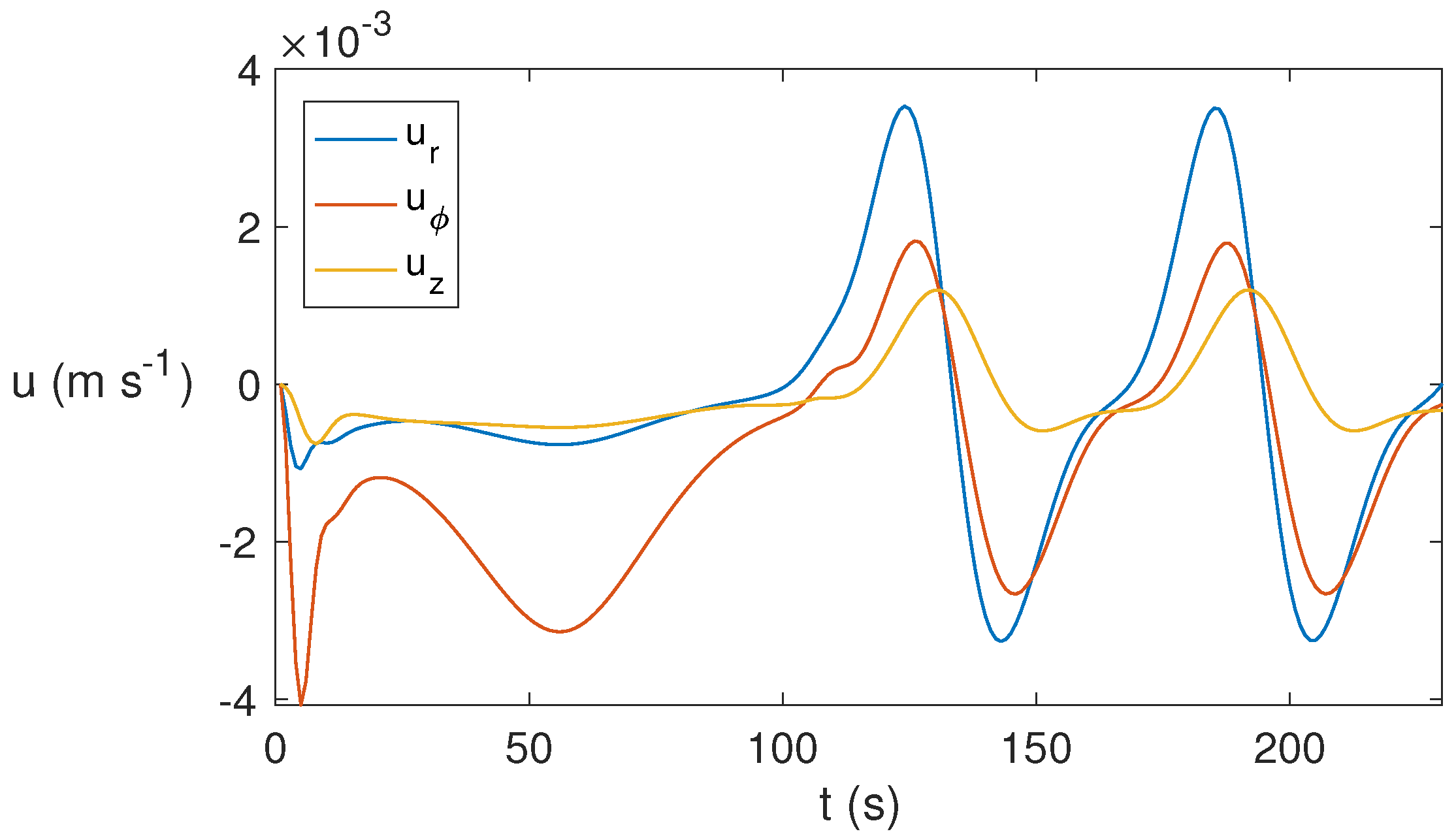
As time evolves, the 3D state found becomes periodic, as shown in Figure 12 that displays the temporal evolution of the three velocity components at the point $(0.0069,0,0.0034)$. From $t=115$ s, the periodic pattern appears. This behavior is found for $\mathsf{\Omega }$ around ${\displaystyle \frac{\pi }{30}}$ s⁻¹ but not for lower rotation rates, for which the state evolves essentially to a conductive state.

Figure 12. Temporal evolution of the velocity components for ethylene glycol for MW at 2.45 GHz and 80 W for $\mathsf{\Omega }={\displaystyle \frac{\pi }{30}}{s}^{-1}$ at the point $(0.0069,0,0.0034)$. A periodic behavior is reported from $t=115$ s.

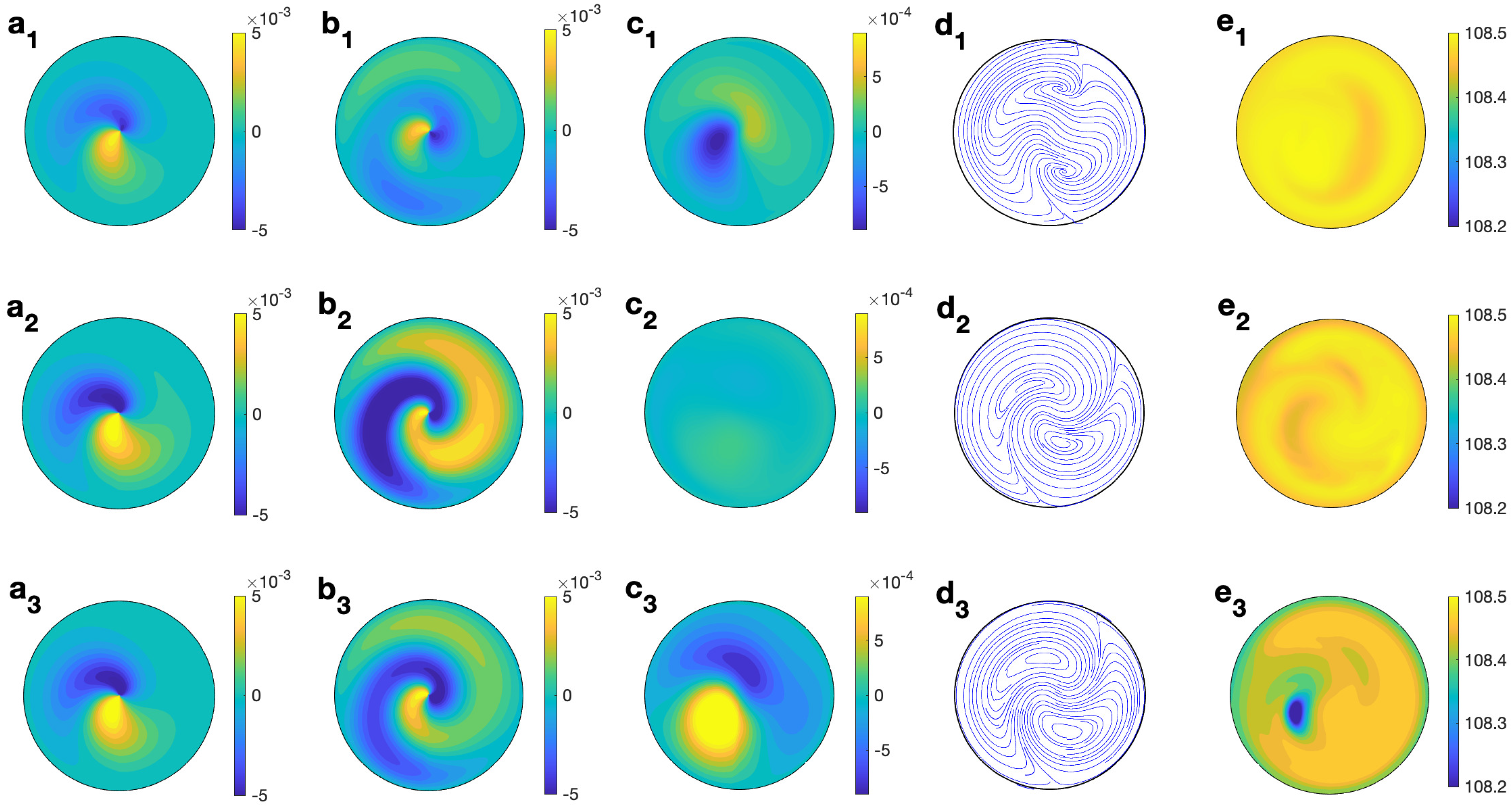
Figure 13 (left column) shows the profiles for velocity, temperature, and microwave power absorption at $\varphi =0$ $(\varphi =\pi )$, $\mathsf{\Omega }=0$ s⁻¹, and $t=120$ s. As observed, at that time the temperature is almost homogeneous around 108 °C in the cell (Figure 13 (e₁)). There is very little contribution from the microwave-power-absorption term (Figure 13 (f₁)), so temperature is not expected to rise more and the radial and vertical velocity components (Figure 13 (a₁ and c₁)) are very small. The azimuthal component is null.

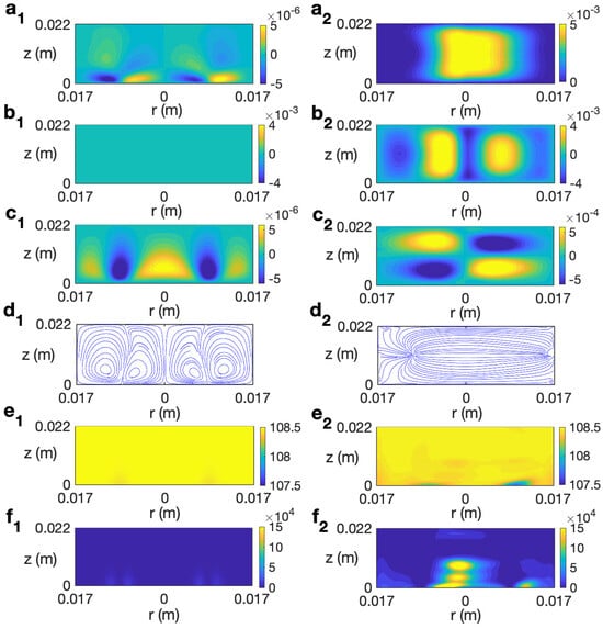
Figure 13. Contours of the predicted velocity, temperature, and microwave power absorption Q for ethylene glycol for MW at 2.45 GHz and 80 W at $\varphi =0$ $(\varphi =\pi )$ for $t=120$ s. (a₁–f₁) $\mathsf{\Omega }=0$ s⁻¹; (a₂–f₂) $\mathsf{\Omega }={\displaystyle \frac{\pi }{30}}$ s⁻¹. From top to bottom: $u_r$, $u_{\varphi }$, $u_z$, streamlines, T, and Q.

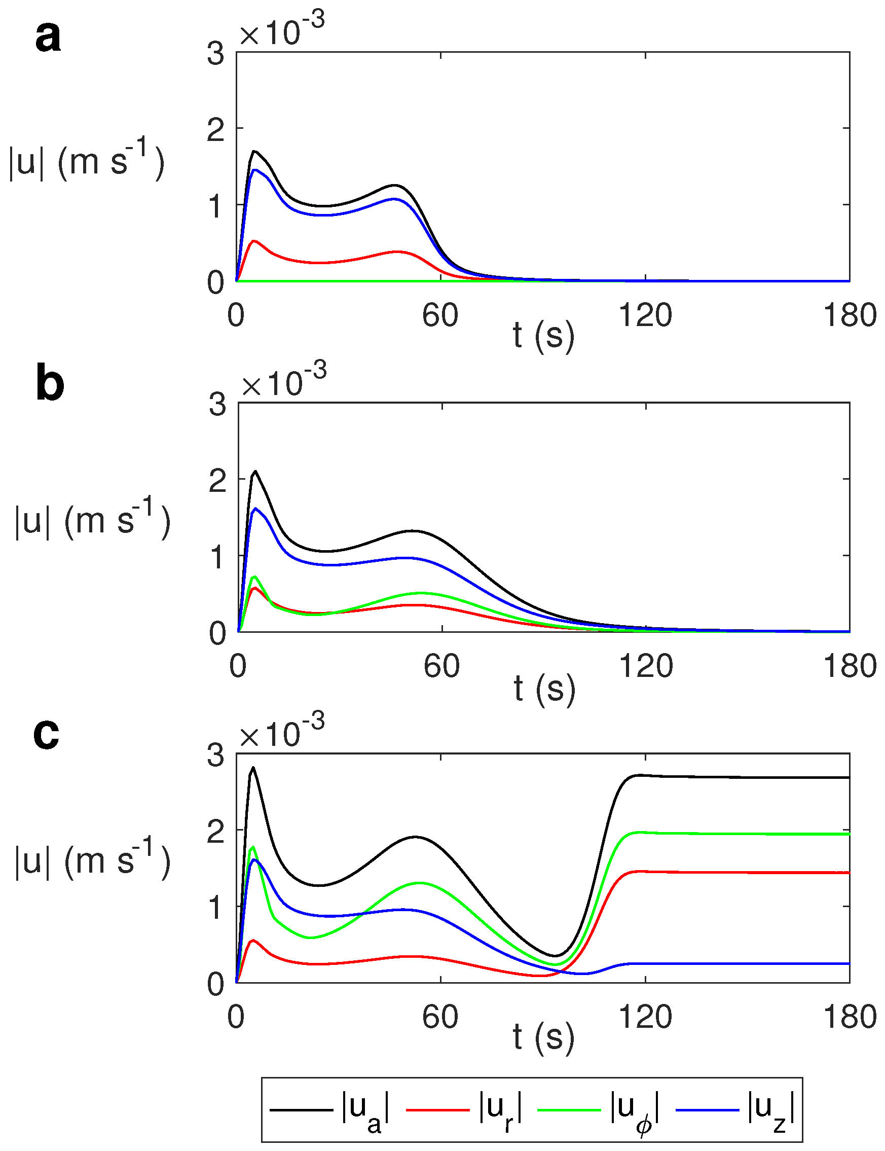
Figure 14 displays the temporal evolution of the average velocity and the average of each velocity component for $\mathsf{\Omega }=0$ s⁻¹, $\mathsf{\Omega }={\displaystyle \frac{\pi }{80}}$ s⁻¹, and $\mathsf{\Omega }={\displaystyle \frac{\pi }{30}}$ s⁻¹. For the cases $\mathsf{\Omega }=0$ s⁻¹ (Figure 14a) and $\mathsf{\Omega }={\displaystyle \frac{\pi }{80}}$ s⁻¹ (Figure 14b), the velocity falls to zero at $t=90$ s in the non-rotation case and around $t=150$ s in the case $\mathsf{\Omega }={\displaystyle \frac{\pi }{80}}$ s⁻¹. The state becomes essentially conductive.

Figure 14. Time evolution of the average velocity $|{\mathbf{u}}_a|$ and the average radial $|{\mathbf{u}}_r|$, azimuthal $|{\mathbf{u}}_{\varphi }|$, and vertical $|{\mathbf{u}}_z|$ velocities for ethylene glycol for MW at 2.45 GHz and 80 W at different values of $\mathsf{\Omega }$. (a) $\mathsf{\Omega }=0$ s⁻¹; (b) $\mathsf{\Omega }={\displaystyle \frac{\pi }{80}}$ s⁻¹; (c) $\mathsf{\Omega }={\displaystyle \frac{\pi }{30}}{s}^{-1}$.

For $\mathsf{\Omega }={\displaystyle \frac{\pi }{30}}$ s⁻¹, the situation is different. As observed in Figure 14c, till 90 s the behavior is quite similar to the case with lower rotation but with a stronger azimuthal velocity. The state that stabilizes after that time is the periodic state described above. This periodicity justifies the constant profiles for the average velocities displayed in Figure 14c from $t=115$ s.

Figure 13 (right column) shows the profiles for velocity, temperature, and microwave power absorption at $\varphi =0$ $(\varphi =\pi )$, $\mathsf{\Omega }={\displaystyle \frac{\pi }{30}}$ s⁻¹, and $t=120$ s. Non-axisymmetry is seen in all of the profiles displayed. The temperature profile (Figure 13 (e₂)) presents some heterogeneities at lower levels, that consequently affect the profile of the microwave power absorption (Figure 13 (f₂)). The magnitude of the velocity components is of the order ${10}^{-3}$ m/s (Figure 13 (a₂–c₂)). Profiles are plotted at $\varphi =0$ $(\varphi =\pi )$ but they change from one angle to another as the state is non-axisymmetric. To give a better idea of the 3D behavior of the flow, Figure 15 displays the contours of the predicted velocity and temperature for ethylene glycol for MW at 2.45 GHz and 80 W at different values of z for $t=120$ s and $\mathsf{\Omega }={\displaystyle \frac{\pi }{30}}$ s⁻¹.

Figure 15. Contours of the predicted velocity and temperature for ethylene glycol for MW at 2.45 GHz and 80 W at different values of z for $t=120$ s and $\mathsf{\Omega }={\displaystyle \frac{\pi }{30}}$ s⁻¹. (a₁–e₁) $z=0.02$ m; (a₂–e₂) $z=0.0105$ m; (a₃–e₃) $z=0.005$ m. From left to right: $u_r$, $u_{\varphi }$, $u_z$, streamlines, and T.

The combined effect of radial velocity (Figure 15 (a₁–a₃)) and azimuthal velocity (Figure 15 (b₁–b₃)) is better described in the velocity field shown in Figure 15 (d₁–d₃), where a clockwise motion is observed, that changes to a counterclockwise motion on its way through the center of the cell. This movement is combined with the vertical motion, up and down, in the upper and lower levels (Figure 15 (c₁–c₃)). Temperature is essentially 108 °C at every height (Figure 15 (e₁–e₃)), with some small variations at lower levels.

4. Conclusions

In this work, the effect of rotation during the heating process of a solvent due to radial microwave irradiation has been studied numerically. Two liquids with different properties, water and ethylene glycol, were considered.

We have developed a mathematical model based on a spectral collocation method to simulate and predict the behavior of the fluid.

There are many codes which are commercially available to address the numerical problem of microwave heating in fluids such as ANSYS Multiphysics, and COMSOL Multiphysics, among others. Some studies using these methods can be found in Refs. [8,9,10]. All these commercial packages use the finite element method (FEM). Some studies have developed numerical codes to model microwave heating in fluids. The most commonly used computational methods have been the finite element method (FEM), finite volume method (FVM), and finite difference (FD) [11,12,13]. Our work is the first approach to the problem using spectral methods.

The results show that the higher the rotation rate is, the faster the state becomes fully 3D, showing that the bifurcation occurs earlier in time for fluids with lower viscosity, as observed for water, which is less viscous than ethylene glycol.

The fully 3D simulations performed with water agree with the axisymmetric simulations performed in [21] and conclude that, in the case of radial irradiation, rotation does not improve the temperature homogeneity in the sample; indeed an increase in non-uniformity of temperature is observed. This result points out that radial irradiation and rotation are not a suitable combination to reach temperature homogenization, required in many applications, contrary to what is reported for domestic household microwave systems, where the radiation is highly non-axisymmetric and rotation increases the mixing in liquids and improves the temperature homogeneity in the sample [17,18].

When we combine a high susceptibility to microwave irradiation with higher viscosity, as in the case of ethylene glycol, the flow remains axisymmetric for a long time and is similar to the non-rotation case (except for the azimuthal velocity), and it becomes 3D when it has almost reached a stationary homogeneous maximum temperature all along the cell. When bifurcation occurs in this case, a periodic state is achieved.

The results presented in this work show the complexity of the flow developed when rotation is added to radial microwave irradiation and how it is fully dependent on the dielectric and thermophysical properties of the solvent, which is relevant in industrial applications. The 3D spatio-temporal description of the behavior of the flow provided with the simulations performed has a remarkable interest for laboratory experiments in order to fully understand the thermal processes when rotation is added to radial microwave irradiation.

As future work, it would be interesting to perform a more systematic study of the effect of rotation on microwave heating depending on the characteristics of the fluid (viscosity, specific heat capacity, etc.) and also to study the effect of other parameters such as the size of the sample or the frequency of the microwave irradiation when rotation is considered in the system.

References

- Gabriel, C.; Gabriel, S.; Grant, E.H.; Halstead, B.S.; Mingos, D.M.P. Dielectric Parameters Relevant to Microwave Dielectric Heating. Chem. Soc. Rev. 1998, 27, 213–224. [Google Scholar] [CrossRef]
- Oliveira, M.E.C.; Franca, A.S. Microwave Heating of Foodstuffs. J. Food Eng. 2002, 53, 347–359. [Google Scholar] [CrossRef]
- Campañone, L.A.; Zaritzky, N.E. Mathematical Modeling and Simulation of Microwave Thawing of Large Solid Foods Under Different Operating Conditions. Food Bioprocess. Technol. 2010, 3, 813–825. [Google Scholar] [CrossRef]
- Mao, W.; Watanabe, M.; Sakai, N. Analysis of Temperature Distributions in Kamaboko During Microwave Heating. J. Food Eng. 2005, 71, 187–192. [Google Scholar] [CrossRef]
- Campañone, L.A.; Paola, C.A.; Mascheroni, R.H. Modeling and Simulation of Microwave Heating of Foods Under Different Process Schedules. Food Bioprocess. Technol. 2012, 5, 738–749. [Google Scholar] [CrossRef]
- Fan, D.; Li, C.; Li, Y.; Chen, W.; Zhao, J.; Hu, M.; Zhang, H. Experimental Analysis and Numerical Modeling of Microwave Reheating of Cylindrically Shaped Instant Rice. Int. J. Food Eng. 2014, 10, 59–67. [Google Scholar] [CrossRef]
- Navarro, M.C.; Burgos, J. A Spectral Method for Numerical Modeling of Radial Microwave Heating in Cylindrical Samples with Temperature Dependent Dielectric Properties. Appl. Math. Model. 2017, 43, 268–278. [Google Scholar] [CrossRef]
- Yousefi, T.; Mousavi, S.A.; Saghir, M.Z.; Farahbakhsh, B. An Investigation on the Microwave Heating of Flowing Water: A Numerical Study. Int. J. Therm. Sci. 2013, 71, 118–127. [Google Scholar] [CrossRef]
- Salvi, D.; Boldor, D.; Aita, G.M.; Sabliov, C.M. COMSOL Multiphysics Model for Continuous Flow Microwave Heating Liquids. J. Food Eng. 2011, 104, 422–429. [Google Scholar] [CrossRef]
- Tuta, S.; Palazoglu, T.K. Finite Element Modeling of Continuous-Flow Microwave Heating of Fluid Foods and Experimental Validation. J. Food Eng. 2017, 192, 79–92. [Google Scholar] [CrossRef]
- Ratanadecho, P.; Aoki, K.; Akahori, M. A Numerical and Experimental Investigation of the Modeling of Microwave Heating for Liquid Layers Using a Rectangular Wave Guide (Effects of Natural Convection and Dielectric Properties). Appl. Math. Model. 2002, 26, 449–472. [Google Scholar] [CrossRef]
- Cha-Um, W.; Rattanadecho, P.; Pakdee, W. Experimental and Numerical Analysis of Microwave Heating of Water and Oil Using a Rectangular Wave Guide: Influence of Sample Sizes, Position, and Microwave Power. Food Bioprocess Technol. 2011, 4, 544–558. [Google Scholar] [CrossRef]
- Yakovlev, V.V. Examination of Contemporary Electromagnetic Software Capable of Modeling Problems of Microwave Heating, Advances in Microwave and Radio Frequency Processing; Willert-Porada, M., Ed.; Springer: Berlin/Heidelberg, Germany, 2005; pp. 178–190. [Google Scholar]
- Navarro, M.C.; Diaz-Ortiz, A.; Prieto, P.; de la Hoz, A. A Spectral Numerical Model and an Experimental Investigation on Radial Microwave Irradiation of Water an Ethanol in a Cylindrical Vessel. Appl. Math. Model. 2019, 66, 680–694. [Google Scholar] [CrossRef]
- Liu, S.; Fukuoka, M.; Sakai, N. A finite element model for simulating temperature distributions in rotating microwave heating. J. Food Eng. 2013, 115, 49–62. [Google Scholar] [CrossRef]
- Pitchai, K.; Chen, J.; Birla, S.; Gonzalez, R.; Jones, D.; Subbiah, J. A microwave heat transfer model for a rotating multi-component meal in a domestic oven: Development and validation. J. Food Eng. 2014, 128, 60–71. [Google Scholar] [CrossRef]
- Zhu, H.; He, J.; Hong, T.; Yang, W.; Wu, Y.; Yang, Y.; Huang, K. A rotary radiation structure for microwave heating uniformity improvement. Appl. Therm. Eng. 2018, 141, 648–658. [Google Scholar] [CrossRef]
- Topcam, H.; Karatas, O.; Erol, B.; Erdogdu, F. Effect of rotation on temperature uniformity of microwave processed low-high viscosity liquids: A computational study with experimental validation. Innov. Food Sci. Emerg. Technol. 2020, 60, 102306. [Google Scholar] [CrossRef]
- Khaghanikavkani, E.; Farid, M.M.; Holdem, J.; Williamson, A. Microwave pyrolysis of plastic. J. Chem. Eng. Process Technol. 2013, 4, 1000150. [Google Scholar] [CrossRef]
- Kouzaev, G.A. A Method and Apparatus for Separate Supply of Microwave and Mechanical Energies to Liquid Reagents in Coaxial Rotating Chemical Reactors. UK Patent Application GB1704095.7, 15 March 2017. [Google Scholar]
- Chatterjee, S.; Basak, T.; Das, S.K. Microwave driven convection in a rotating cylindrical cavity: A numerical study. J. Food Eng. 2007, 79, 1269–1279. [Google Scholar] [CrossRef]
- Balanis, C.A. Advanced Engineering Electromagnetics; Wiley: New York, NY, USA, 1989. [Google Scholar]
- Canuto, C.; Hussain, M.Y.; Quarteroni, A.; Zang, T.A. Spectral Methods in Fluid Dynamics; Springer: Berlin/Heidelberg, Germany, 1988. [Google Scholar]
- Herrero, H.; Mancho, A.M. On pressure boundary conditions for thermoconvective problems. Int. J. Numer. Meth. Fluids 2002, 39, 391–402. [Google Scholar] [CrossRef]
- Mercader, I.; Batiste, O.; Alonso, A. An Efficient Spectral Code for Incompressible Flows in Cylindrical Geometries. Comput. Fluids 2010, 39, 215–224. [Google Scholar] [CrossRef]
- Horikoshi, S.; Matsuzaki, S.; Mitani, T.; Serpone, N. Microwave frequency effects on dielectric properties of some common solvents and on microwave-assisted syntheses: 2-Allyphenol and the C12–C2–C12 Gemini Surfactant. Radiat. Phys. Chem. 2012, 81, 1885–1895. [Google Scholar] [CrossRef]
- Faghri, A.; Zhang, Y. Transport Phenomena in Multiphase Systems; Elsevier: Burlington, MA, USA, 2006. [Google Scholar]
- Faghri, A.; Zhang, Y.; Howell, J. Advanced Heat and Mass Transfer; Global Digital Press: Columbia, OH, USA, 2010. [Google Scholar]
- Vargaftik, N.B. Handbook of Physical Properties of Liquids and Gases; Hemisphere: New York, NY, USA, 1975. [Google Scholar]
- Navarro, M.C.; Castaño, D. Microwave irradiation and conventional heating: A comparison using in silico experiments with water and ethylene glycol. Heat Transf. Res. 2022, 53, 73–91. [Google Scholar] [CrossRef]
- Navarro, M.C. Water, Toluene, Methanol and Ethanol Under Microwave Irradiation: Numerical Simulations of the Effect of the Vessels Size. J. Heat Transf. 2020, 142, 102104. [Google Scholar] [CrossRef]
Disclaimer/Publisher’s Note: The statements, opinions and data contained in all publications are solely those of the individual author(s) and contributor(s) and not of MDPI and/or the editor(s). MDPI and/or the editor(s) disclaim responsibility for any injury to people or property resulting from any ideas, methods, instructions or products referred to in the content. |
© 2025 by the authors. Licensee MDPI, Basel, Switzerland. This article is an open access article distributed under the terms and conditions of the Creative Commons Attribution (CC BY) license (https://creativecommons.org/licenses/by/4.0/).