Stability Study for an Age-Structured Epidemic Model with Latent Phase, Relapse and Nonlinear Infection Rate

Abstract

This paper is dedicated to the analytical investigation of the global dynamics of an SEIR epidemiological model that incorporates latency age (the time spent by an individual in the exposed class before becoming infectious) and a general nonlinear incidence rate. In this model, to reflect the dependence of disease progress on the latency age, the exposed class is structured by the latency age, and the rate at which the latent individual becomes infected, and the removal rate are assumed to depend on the latency age. By analyzing the characteristic equations associated with each equilibrium, we study the local stability of both the disease-free and endemic steady states of the model. Moreover, it is proven that the semiflow generated by this system is asymptotically smooth, and if the basic reproduction number is greater than unity, the system is uniformly persistent. Furthermore, based on Lyapunov functional and LaSalle’s invariance principle, the global dynamics of the model are established. It is obtained that if the basic reproduction number is less than unity, the disease-free steady state is globally asymptotically stable and hence the disease dies out; however, if the basic reproduction number is greater than unity, the endemic steady state is globally asymptotically stable, and the disease persists. Numerical simulations are carried out to illustrate the main analytic results.

1. Introduction

The emergence and persistence of infectious diseases remain among the most pressing challenges for public-health systems and global development. Epidemics not only endanger human lives but also generate severe social and economic consequences, which makes their prevention and control a priority for researchers and decision-makers alike. In this context, mathematical models have become a very important tool, providing a rigorous way to describe disease mechanisms and to predict their behaviors. Such models allow us to identify the impact of various epidemiological factors, explore potential interventions and strategies for control, and uncover the dynamics behind complex phenomena such as the latency period, the relapse phase, and the mechanism of transmission. The approach in this field is the use of compartmental models, which divide the population into subgroups based on their health status and the rules governing transitions between them. Simplifying biological processes into well-defined compartments makes it possible to study the interaction between susceptible, exposed, infectious, and recovered individuals, and to evaluate the conditions that favor or prevent the infectious (see, e.g., [1,2,3,4,5]).

The SIR model, introduced by Kermack and McKendrick [6] in 1927, represents the cornerstone of compartmental modeling. In its original form, the population is divided into three groups: susceptible, infectious, and recovered individuals. This simple model was designed to analyze the dynamics of diseases that provide permanent immunity after infection, such as measles or chickenpox. Since then, the SIR model has been extended in numerous versions to understand the complexities of real-world diseases better. These developments have generated a wide variety of models that continue to guide public-health authorities to design effective strategies of control and prevention of the spread of disease, some of which are described in [7,8,9,10,11] and references therein.

While the classical SIR model has provided fundamental insights, it does not capture important features observed in many infectious diseases. In particular, many infectious diseases involve a latency period during which individuals are infected but not yet infectious [12]. To address this limitation, the SIR model has been extended by introducing a latent compartment, leading to the SEIR model. This extension makes it possible to describe more accurately the transmission dynamics of infectious diseases with a significant latency period (see, e.g., [13,14,15,16]). Moreover, clinical evidence shows that some recovered individuals may lose their immunity and relapse into an infectious state, a phenomenon that further complicates disease dynamics [17,18,19,20,21]. Incorporating such mechanisms is essential for developing models that better reflect reality and for supporting effective public-health interventions.

Most of these models are based on differential equations (ODEs), which assume that all individuals in different categories have the same waiting time. However, they also have clear limitations. These models do not explicitly take into account the time individuals spend in different stages of infection. As a result, important epidemiological factors such as the latency period or the delay before becoming infectious are often ignored. This simplification makes ODE models less accurate for such infectious diseases where the latency age plays an essential role. For example, latent tuberculosis can remain in the inactive stage without causing disease for months, years, or even decades before becoming infectious, potentially developing into a severe stage, highly contagious, and deadly disease if left untreated or incompletely treated [22,23]. This limitation motivates the use of age-structured epidemic models, which represent either the chronological age of individuals or the period they have already spent in a particular disease stage (see, e.g., [1,24,25,26,27,28]). In particular, models that incorporate latency age can represent more accurately the progression of exposed individuals through the latency period. This structure allows us to capture variability in the timing of infectiousness, to model delays more realistically. As a result, age-structured models incorporating the latency period offer a more reliable framework for analyzing complex infectious diseases. For instance, in viral-bacterial structured models that account for such delays (latent period), see, e.g., [29].

Motivated by previous works, this study focuses on the global dynamical behavior of an SEIR age-structured epidemic model that incorporates latency age, relapse, and a general nonlinear incidence rate. The model is particularly well-suited for infectious diseases that involve latent periods and relapse, such as tuberculosis and herpes virus infection. Its novelty lies in the fact that both the latency period and relapse mechanism are considered, while at the same time accounting for nonlinear transmission. Furthermore, since recovered individuals are allowed to relapse, we then assume that a fraction $0<p<1$ of relapsed individuals become re-infectious again, while the remaining fraction $1-p$ re-enter the latent class.

To create our epidemic model, we divide the population into four subsets: susceptible, exposed, infected, and recovered. Let $S\left(t\right)$ denote the size of the susceptible individual at time t; $e(t,a)$ the density of exposed individuals who are infected but not yet infectious at time t and latency age a; $I\left(t\right)$ the number of infected individual at time t; and $R\left(t\right)$ the size of recovered individuals at time t.

The model is based on the following assumptions:

Infection mechanism: Susceptible individuals become infected through contact with infectious individuals with incidence described by a general nonlinear function $S\left(t\right)f\left(I\right(t\left)\right)$.

Newly infected individuals are assumed to pass through the latency period (i.e., the period from infection to the onset of infectiousness) before they can transmit the disease.

Progressing from latency: Exposed individuals, who are infected but cannot yet become infectious, progress to the infected class at age-dependent rate $\delta \left(a\right)$. Thus, the total rate at which latent individuals become is given by ${\displaystyle {\int }_0^{\infty }\delta \left(a\right)e(t,a)da}$.

Recovery: Infected individuals are recovering at rate $\alpha$. Therefore, the total rate at which the infected individuals become recovered is estimated as $\alpha I\left(t\right)$.

Relapse: After recovery, individuals may experience relapse. This occurs at a rate $\sigma$. Also, we assume that a fraction $0<p<1$ of relapsed individuals become re-infectious again at rate $p\sigma R\left(t\right)$, while the remaining fraction $1-p$ re-enter the latent class at rate $(1-p)\sigma R\left(t\right)$.

Mortality: Susceptible, latent, infected, and recovered individuals removed at a constant rate $\mu$.

Therefore, the disease spread model, according to the above assumptions, is represented as follows:

$$\left\{\begin{array}{c}{\displaystyle \frac{dS\left(t\right)}{dt}=\mathrm{\Pi }-\mu S\left(t\right)-f\left(I\left(t\right)\right)S\left(t\right),}\hfill \\ {\displaystyle \frac{\partial e(t,a)}{\partial t}+\frac{\partial e(t,a)}{\partial a}=-(\mu +\delta \left(a\right))e(t,a),}\hfill \\ {\displaystyle \frac{dI\left(t\right)}{dt}={\int }_0^{\infty }\delta \left(a\right)e(t,a)da+p\sigma R\left(t\right)-(\mu +\alpha )I\left(t\right),}\hfill \\ {\displaystyle \frac{dR\left(t\right)}{dt}=\alpha I\left(t\right)-(\mu +\sigma )R\left(t\right),}\hfill \end{array}\right.$$

(1)

with boundary conditions

$${\displaystyle e(t,0)=f\left(I\right(t\left)\right)S\left(t\right)+(1-p)\sigma R\left(t\right):=J\left(t\right),}$$

(2)

and initial condition, by biological reasons, are the positive continuous functions

$$S\left(0\right)=S_0,e(0,a)=e_0\left(a\right),I\left(0\right)=I_0,\mathrm{and}R\left(0\right)=R_0.$$

(3)

For model (1)–(3), there should be an inherent relationship between the initial values and the boundary values for the partial differential equations, i.e., $e(0,0)=e_0\left(0\right)$. Thus, throughout the remainder of this paper, we always assume

$$e_0\left(0\right)=f\left(I_0\right)S_0+(1-p)\sigma R_0.$$

(4)

The structure of this paper is organized as follows: Section 2 provides some preliminary results for system (1)–(3), addressing the well-posedness of solutions, the existence of the disease-free and endemic steady states, and the asymptotic smoothness property of the semiflow $\mathrm{\Phi }$. In Section 3, we establish the local and global stability of both steady states of system (1)–(3). Section 4 is devoted to numerical simulations that validate our theoretical results and shed light on the role of key parameters in shaping disease transmission dynamics. Finally, Section 5 concludes this work and discusses the results.

2. Preliminaries

2.1. Assumptions and Notations

To investigate this paper, we will proceed under the following assumptions:

Assumption 1. 

For system (1)–(3), we assume that:

• The parameters satisfy: Π, μ, α, $\sigma >0$, and $p\in [0,1]$;
• The function $\delta (·)\in L_{+}^{\infty }(0,\infty )$, the nonnegative cone of the Banach space consisting of essentially bounded functions from $(0,\infty )$ into ${\mathbb{R}}_{+}$.

Assumption 2. 

The nonlinear incidence function f is assumed to satisfy:

For $\xi \in {\mathbb{R}}_{+}$, $f\in {\mathcal{C}}^2$, the set of twice continuously differentiable functions from $(0,\infty )$ into ${\mathbb{R}}_{+}$, such that $f\left(0\right)=0$, $f^{\prime }\left(\xi \right)\ge 0$, and $f^{″}\left(\xi \right)\le 0$.

For any function $\pi \in L_{+}^{\infty }(0,\infty )$, we denote

$$\underline{\pi }:=ess\underset{a\in {\mathbb{R}}_{+}}{inf}\pi \left(a\right)<+\infty ,\mathrm{and}\overline{\pi }:=ess\underset{a\in {\mathbb{R}}_{+}}{sup}\pi \left(a\right)<+\infty .$$

Remark 1. 

From Assumption 2, we can easily notice that f is always a nonnegative function for all $\xi \in {\mathbb{R}}_{+}$, Moreover, with the help of Taylor’s Theorem, we have

$$f^{\prime }\left(\xi \right)\xi \le f\left(\xi \right)\le f^{\prime }\left(0\right)\xi .$$

(5)

The following are some examples of incidence functions that conform to the Assumption 2:

• The bilinear incidence $Sf\left(I\right)$, where $f\left(I\right)=\beta I$ and $\beta >0$ denotes the transmission rate (see, e.g., [30]), which is extensively used in modeling the transmission of infectious diseases. However, it does not always accurately conform to the complex epidemiological factors influencing the transmission of a disease.
• Saturated incidence rate given by $Sf\left(I\right)$ with $f\left(I\right)={\displaystyle \frac{\beta I}{1+\alpha I}}$, where $\alpha ,\beta >0$ (see, e.g., [31]), This form approaches a saturation threshold as I becomes large, where $\beta I$ represents the infection force, and $1/(1+\alpha I)$ denotes the inhibition effect from the behavioral change in susceptible individuals when their number increases or from the crowding effect of the infective individuals.

2.2. Volterra Formulation

With the help of the characteristic method ([32] Chapter 1), solving the second partial differential equations of system (1) with boundary condition (2) and initial condition (3) along the characteristic lines $t-a=const$, gives

$$e(t,a)=\left\{\begin{array}{cc}J(t-a)\zeta \left(a\right),\hfill & \hfill t>a,\\ {\displaystyle e_0(a-t)\frac{\zeta \left(a\right)}{\zeta (a-t)},}\hfill & \hfill t\le a,\end{array}\right.$$

(6)

where $J\left(t\right)$ is defined by (2), and $\zeta :{\mathbb{R}}_{+}⟶{\mathbb{R}}_{+}$ is given as

$$\zeta \left(a\right)=e^{{\displaystyle -{\int }_0^a\psi \left(s\right)ds}},$$

(7)

with

$$\psi (·)=\mu +\delta (·).$$

(8)

2.3. Well-Posedness

Define the following space

$$\mathbb{X}={\mathbb{R}}_{+}\times L_{+}^1(0,\infty )\times {\mathbb{R}}_{+}\times {\mathbb{R}}_{+},$$

equipped with the norm

$$\parallel ({\omega }_1,{\omega }_2(·),{\omega }_3,{\omega }_4){\parallel }_{\mathbb{X}} = |{\omega }_1| + \parallel {\omega }_2{(·)\parallel }_1 +| {\omega }_3| + |{\omega }_4|.$$

where $L_{+}^1(0,+\infty )$ is the set of integrable functions from $(0,+\infty )$ into ${\mathbb{R}}_{+}$, and ${\parallel · \parallel }_1$ denotes the $L^1$-norm.

According to the standard theory of functional differential equations (see, e.g., [33,34]), system (1)–(3) admits a unique continuous solution in $\mathbb{X}$ if the initial condition $(S_0,e_0(·),$$I_0,R_0)\in \mathbb{X}$ satisfies the condition (4).

Therefore, we can define a continuous semiflow $\mathrm{\Phi }:{\mathbb{R}}_{+}\times \mathbb{X}\to \mathbb{X}$ as follows:

$$\mathrm{\Phi }(t,x_0)=(S\left(t\right),e(t,·),I\left(t\right),R\left(t\right)),t\ge 0,x_0\in \mathbb{X}.$$

(9)

Hence

$$\parallel \mathrm{\Phi }(t,x_0){\parallel }_{\mathbb{X}}=\parallel (S\left(t\right),e(t,·),I\left(t\right),R\left(t\right)){\parallel }_{\mathbb{X}}=S\left(t\right)+{\int }_0^{\infty }e(t,a)da+I\left(t\right)+R\left(t\right).$$

Furthermore, we set

$$\mathrm{\Sigma }=\left\{(S,e,I,R)\in \mathbb{X}:S\left(t\right)+{\int }_0^{\infty }e(t,a)da+I\left(t\right)+R\left(t\right)\le {\displaystyle \frac{\mathrm{\Pi }}{\mu }}\right\}.$$

Now, we can introduce the following results:

Proposition 1. 

Considering system (1)–(3), then we have

(i)

Σ is positively invariant for ${\left\{\mathrm{\Phi }(t,x_0)\right\}}_{t\ge 0}$, i.e., $\mathrm{\Phi }(t,x_0)\in \mathrm{\Sigma }$, for $x_0\in \mathrm{\Sigma }$ and $t\ge 0$;

(ii)

${\left\{\mathrm{\Phi }(t,x_0)\right\}}_{t\ge 0}$ is point-dissipative and Σ attract all points in $\mathbb{X}$.

Proof. 

Define the total population

$$N\left(t\right):=S\left(t\right)+{\int }_0^{\infty }e(t,a)da+I\left(t\right)+R\left(t\right).$$

Differentiate $N\left(t\right)$ with respect to time t and using the equations of system (1)–(3), it yields

$$\begin{array}{cc}\hfill {\displaystyle \frac{N\left(t\right)}{dt}}& ={\displaystyle \frac{S\left(t\right)}{dt}}+{\displaystyle \frac{d}{dt}}{\int }_0^{\infty }e(t,a)da+{\displaystyle \frac{I\left(t\right)}{dt}}+{\displaystyle \frac{R\left(t\right)}{dt}}\hfill \\ & =\left(\mathrm{\Pi }-\mu S-f\left(I\right)S\right)+\left(e(t,0)-{\int }_0^{\infty }(\mu +\delta \left(a\right))e(t,a)da\right)\hfill \\ & +\left({\int }_0^{\infty }\delta \left(a\right)e(t,a)da+p\sigma R-(\mu +\alpha )I\right)+\left(\alpha I-(\mu +\sigma )R\right).\hfill \end{array}$$

Hence, we can have

$${\displaystyle \frac{N\left(t\right)}{dt}}=\mathrm{\Pi }-\mu \left(S+{\int }_0^{\infty }e(t,a)da+I+R\right)=\mathrm{\Pi }-\mu N\left(t\right).$$

Therefore $N\left(t\right)$ satisfies

$${\displaystyle \frac{N\left(t\right)}{dt}}=\mathrm{\Pi }-\mu N\left(t\right).$$

(10)

By solving Equation (10), we obtain

$$N\left(t\right)=N\left(0\right)e^{-\mu t}+{\displaystyle \frac{\mathrm{\Pi }}{\mu }}\left(1-e^{-\mu t}\right),\mathrm{for}\mathrm{all}t\ge 0.$$

Therefore, it yields

$$\underset{t\to \infty }{lim}N\left(t\right)={\displaystyle \frac{\mathrm{\Pi }}{\mu }},N\left(t\right)\le max\{N\left(0\right),\mathrm{\Pi }/\mu \}\mathrm{for}\mathrm{all}t\ge 0.$$

(i)

Positive invariance of Σ. Let $x_0\in \mathrm{\Sigma }$, so $N\left(0\right)\le \mathrm{\Pi }/\mu$. Thus, we can have $N\left(t\right)\le \mathrm{\Pi }/\mu$ for all $t\ge 0$, which implies that $\mathrm{\Phi }(t,x_0)\in \mathrm{\Sigma }$ for all $t\ge 0$, proving positive invariance.

(ii)

Point-dissipativity and attractivity of Σ. For any $x_0\in \mathbb{X}$, we have $N\left(t\right)$ satisfies

$$N\left(t\right)=N\left(0\right)e^{-\mu t}+{\displaystyle \frac{\mathrm{\Pi }}{\mu }}\left(1-e^{-\mu t}\right).$$

Hence $N\left(t\right)\to \mathrm{\Pi }/\mu$ as $t\to \infty$. Therefore, we can easily deduce that the semiflow is point-dissipative and Σ attracts all points in $\mathbb{X}$.

□

Proposition 2. 

Let $x_0\in \mathbb{X}$ with $\parallel x_0{\parallel }_{\mathbb{X}}\le M$ for some constant $M\ge {\displaystyle \frac{\mathrm{\Pi }}{\mu }}$. Then the following statements hold true for $t\ge 0$:

(i)

${\displaystyle 0\le S\left(t\right),{\int }_0^{\infty }e(t,a)da,I\left(t\right),R\left(t\right)\le M}$;

(ii)

$e(t,0)\le \left[f^{\prime }\left(0\right)M+(1-p)\sigma \right]M$;

(iii)

${\displaystyle \underset{t\to \infty }{lim\; inf}S\left(t\right)\ge \frac{\mathrm{\Pi }}{\mu +f^{\prime }\left(0\right)M}}$.

Proof. 

Assume $x_0=(S_0,e_0(·),I_0,R_0)\in \mathbb{X}$ satisfies $\parallel x_0{\parallel }_{\mathbb{X}}\le M$ for some $M\ge \mathrm{\Pi }/\mu$.

(i)

Let $N\left(0\right)\le \parallel x_0{\parallel }_{\mathbb{X}}\le M$ and $\mathrm{\Pi }/\mu \le M$, it follows $N\left(t\right)\le M$ for all $t\ge 0$. Hence

$$0\le S\left(t\right),{\int }_0^{\infty }e(t,a)da,I\left(t\right),R\left(t\right)\le M,\forall t\ge 0,$$

which proves (i).

(ii)

Recall the boundary condition $e(t,0)=f\left(I\right(t\left)\right)S\left(t\right)+(1-p)\sigma R\left(t\right)$. Using the fact that $f\left(I\left(t\right)\right)\le f^{\prime }\left(0\right)I\left(t\right)$, we can obtain

$$\begin{array}{cc}\hfill e(t,0)& =f\left(I\right(t\left)\right)S\left(t\right)+(1-p)\sigma R\left(t\right)\hfill \\ & \le f^{\prime }\left(0\right)I\left(t\right)S\left(t\right)+(1-p)\sigma R\left(t\right)\hfill \\ & \le f^{\prime }\left(0\right)M^2+(1-p)\sigma M=\left(f^{\prime }\left(0\right)M+(1-p)\sigma \right)M,\hfill \end{array}$$

because $I\left(t\right),S\left(t\right),R\left(t\right)\le M$. This is exactly statement (ii).

(iii)

From the S-equation in system (1), we obtain

$${\displaystyle \frac{dS\left(t\right)}{dt}}=\mathrm{\Pi }-\mu S\left(t\right)-f\left(I\left(t\right)\right)S\left(t\right),$$

and using $f\left(I\left(t\right)\right)\le f^{\prime }\left(0\right)I\left(t\right)\le f^{\prime }\left(0\right)M$, we obtain the differential inequality

$${\displaystyle \frac{dS\left(t\right)}{dt}}\ge \mathrm{\Pi }-\left(\mu +f^{\prime }\left(0\right)M\right)S\left(t\right).$$

Consider the scalar linear equation

$${\displaystyle \frac{dy\left(t\right)}{dt}}=\mathrm{\Pi }-\left(\mu +f^{\prime }\left(0\right)M\right)y\left(t\right),y\left(0\right)=S_0.$$

Its solution satisfies $y\left(t\right)\to {\displaystyle \frac{\mathrm{\Pi }}{\mu +f^{\prime }\left(0\right)M}}$ as $t\to \infty$, and by the comparison principle, we can conclude that $S\left(t\right)\ge y\left(t\right)$ for all $t\ge 0$. Taking the limit inferior yields

$$\underset{t\to \infty }{lim\; inf}S\left(t\right)\ge {\displaystyle \frac{\mathrm{\Pi }}{\mu +f^{\prime }\left(0\right)M}},$$

which proves (iii).

□

2.4. Asymptotic Smoothness

A continuous semiflow $\mathrm{\Phi }(t,x)$ is called asymptotically smooth if every positively invariant, bounded, and closed set is attracted to a nonempty compact set. To establish this property, we use the approach introduced by Smith and Thieme [35]. The following result will be needed to show that $\mathrm{\Phi }$ is asymptotically smooth:

Lemma 1. 

The function $J\left(t\right)$ defined by (2) is Lipschitz continuous on ${\mathbb{R}}_{+}$.

Proof. 

From system (1)–(3) together with Proposition 2, it follows that $\left|{\displaystyle \frac{dS\left(t\right)}{dt}}\right|\le \mathrm{\Pi }+(\mu +f^{\prime }\left(0\right)M)M:=L_S,\left|{\displaystyle \frac{dI\left(t\right)}{dt}}\right|\le (\overline{\delta }+\mu +\alpha +\sigma p)M:=L_I,$ and $\left|{\displaystyle \frac{dR\left(t\right)}{dt}}\right|\le (\mu +\alpha +\sigma )M:=L_R$. Notice that $L_S$, $L_I$, and $L_R$ are independent of t and the initial conditions.

Now, let $t\in {\mathbb{R}}_{+}$ and $h>0$. Using the definition of $J\left(t\right)$ given by (2), we can obtain

$$\begin{array}{ccc}\hfill \left|J\right(t+h)-J(t\left)\right|& \le & \left|f\right(I(t+h)\left)S\right(t+h)-f(I\left(t\right)\left)S\right(t\left)\right|+(1-p)\sigma \left|R\right(t+h)-R(t\left)\right|\hfill \\ & \le & S\left(t\right)\left|f\right(I(t+h))-f(I\left(t\right)\left)\right|+f\left(I\right(t+h\left)\right)\left|S\right(t+h)-S(t\left)\right|\hfill \\ & & +(1-p)\sigma \left|R\right(t+h)-R(t\left)\right|\hfill \\ & \le & M{f}^{\prime }\left(0\right)(L_I+L_S)+(1-p)\sigma L_R:=L_J.\hfill \end{array}$$

Thus, $J\left(t\right)$ is a Lipschitz continuous function with Lipschitz constant $L_J$. This completes the proof. □

Now, we present the following essential lemmas that will serve as the technical tools for proving the asymptotic smoothness of the semiflow $\mathrm{\Phi }$:

Lemma 2 

([35] Theorem 3.2). The semiflow $\mathrm{\Phi }:{\mathbb{R}}_{+}\times \mathbb{X}\to \mathbb{X}$ is asymptotically smooth if there are maps ${\mathrm{\Phi }}_1,{\mathrm{\Phi }}_2:{\mathbb{R}}_{+}\times \mathbb{X}\to \mathbb{X}\mathrm{such}\mathrm{that}\mathrm{\Phi }(t,x)={\mathrm{\Phi }}_1(t,x)+{\mathrm{\Phi }}_2(t,x)$, and the following statement holds for any bounded and closed set $\mathcal{B}\in \mathcal{X}$, which is forward invariant under Φ

(A1)

${\displaystyle \underset{t\to \infty }{lim}diam{\mathrm{\Phi }}_2(t,\mathcal{B})=0}$;

(A2)

There exists $t_{\mathcal{B}}>0$ such that ${\mathrm{\Phi }}_1(t,\mathcal{B})$ has compact closure for each $t\ge t_{\mathcal{B}}$.

Notice that $\mathbb{X}$ is an infinite dimensional Banach space and $L_{+}^1(0,+\infty )$ is a component of $\mathbb{X}$. Hence, we cannot obtain the pre-compactness only from boundedness. Therefore, to derive the pre-compactness of $\mathbb{X}$, we need to apply the following lemma:

Lemma 3 

([35] Theorem B.2). A set $\mathcal{B}\in L_{+}^1(0,+\infty )$ has a compact closure if the following statements hold

(B1)

${\displaystyle \underset{\varpi \in \mathcal{B}}{sup}{\int }_0^{\infty }\varpi \left(a\right)da<\infty }$;

(B2)

${\displaystyle \underset{\tau \to \infty }{lim}{\int }_{\tau }^{\infty }\varpi \left(a\right)da\to 0\mathit{uniformly}\mathit{in}\varpi \in \mathcal{B}}$;

(B3)

${\displaystyle \underset{\tau \to 0^{+}}{lim}{\int }_0^{\infty }\left|\varpi (a+\tau )-\varpi \left(a\right)\right|da\to 0\mathit{uniformly}\mathit{in}\varpi \in \mathcal{B}}$;

(B4)

${\displaystyle \underset{\tau \to 0^{+}}{lim}{\int }_0^{\tau }\varpi \left(a\right)da\to 0\mathit{uniformly}\mathit{in}\varpi \in \mathcal{B}}$.

Now, we can prove the following result:

Theorem 1. 

The semiflow Φ is asymptotically smooth.

Proof. 

We first define two maps ${\mathrm{\Phi }}_1$ and ${\mathrm{\Phi }}_2$ such that $\mathrm{\Phi }={\mathrm{\Phi }}_1+{\mathrm{\Phi }}_2$, where

$${\mathrm{\Phi }}_1(t,x_0)=(S\left(t\right),e_1(t,·),I\left(t\right),R\left(t\right)),\mathrm{and}{\mathrm{\Phi }}_2(t,x_0)=(0,e_2(t,·),0,0),$$

with

$$e_1(t,a)=\left\{\begin{array}{cc}J(t-a)\zeta \left(a\right),\hfill & t>a,\hfill \\ 0,\hfill & t\le a,\hfill \end{array}\right.\mathrm{and}{e}_2(t,a)=\left\{\begin{array}{cc}0,\hfill & t>a,\hfill \\ e_0(a-t){\displaystyle \frac{\zeta \left(a\right)}{\zeta (a-t)}},\hfill & t\le a,\hfill \end{array}\right.$$

(11)

where $J\left(t\right)$ and $\zeta \left(a\right)$ are given by (2) and (7), respectively. Let $\mathcal{B}\in \mathbb{X}$ be any bounded closed set which is forward invariant under $\mathrm{\Phi }$. We first verify that ${\mathrm{\Phi }}_2$ satisfies condition (A1) in Lemma 2. Therefore, for $x_0\in \mathcal{B}$ satisfying $\parallel x_0{\parallel }_{\mathbb{X}}\le \rho$, we can have

$$\begin{array}{ccc}\hfill \parallel {\mathrm{\Phi }}_2(t,x_0){\parallel }_{\mathbb{X}}& =& \left|0\right|+{\int }_t^{\infty }{e}_0(a-t){\displaystyle \frac{\zeta \left(a\right)}{\zeta (a-t)}}da+\left|0\right|+\left|0\right|\hfill \\ & =& {\int }_0^{\infty }{e}_0\left(a\right){\displaystyle \frac{\zeta (t+a)}{\zeta \left(a\right)}}da\hfill \\ & \le & e^{-\underline{\psi }t}{\parallel x_0\parallel }_{\mathbb{X}}\le \rho e^{-\underline{\psi }t}.\hfill \end{array}$$

Therefore, we have ${\displaystyle \underset{t\to \infty }{lim}{\parallel {\mathrm{\Phi }}_2(t,x_0)\parallel }_{\mathbb{X}}=0}$ which confirms that condition (A1) holds.

Next, we proceed to show that (A2) is satisfied. From Proposition 2, $S\left(t\right)$, $I\left(t\right)$ and $R\left(t\right)$ remain in a compact set $[0,M]$. It remains to show that $e_1(t,a)$ remains in a pre-compact set of $L_{+}^1$ independent of the initial conditions.

Proposition 2 implies that $0\le e_1(t,a)\le (f^{\prime }\left(0\right)M^2+(1-p)\sigma M)e^{-\underline{\psi }a}$, which ensures that (B1), (B2) and (B4) of Lemma 3 are satisfied. We now move to verify condition (B3). To this end, for $\tau \in (0,t)$, we can write

$$\begin{array}{ccc}& & {\int }_0^{\infty }|e_1(t,a+\tau )-e_1(t,a)|da\hfill \\ & & ={\int }_0^{t-\tau }|e_1(t,a+\tau )-e_1(t,a)|da+{\int }_{t-\tau }^t|\underset{=0}{\underbrace{e_1(t,a+\tau )}}-e_1(t,a)|da\hfill \\ & & ={\int }_0^{t-\tau }|J(t-a-\tau )\zeta (a+\tau )-J(t-a)\zeta \left(a\right)|da+{\int }_{t-\tau }^{t}J(t-a)\zeta \left(a\right)da\hfill \\ & & ={\int }_0^{t-\tau }J(t-a-\tau )|\zeta (a+\tau )-\zeta \left(a\right)|da+{\int }_0^{t-\tau }|J(t-a-h)-J(t-a)|\zeta \left(a\right)da\hfill \\ & & +{\int }_{t-\tau }^{t}J(t-a)\zeta \left(a\right)da\hfill \\ & & :={\mathrm{\Gamma }}_1+{\mathrm{\Gamma }}_2+{\mathrm{\Gamma }}_3.\hfill \end{array}$$

(12)

From Proposition 2 together with Remark 1, it yields

$$\begin{array}{ccc}\hfill {\mathrm{\Gamma }}_1& \le & (f^{\prime }\left(0\right)M^2+(1-p)\sigma M)\left[{\int }_0^{t-\tau }\zeta \left(a\right)da-{\int }_0^{t-\tau }\zeta (a+\tau )da\right]\hfill \\ & =& (f^{\prime }\left(0\right)M^2+(1-p)\sigma M)\left[{\int }_0^{t-\tau }\zeta \left(a\right)da-{\int }_{\tau }^t\zeta \left(a\right)da\right]\hfill \\ & =& (f^{\prime }\left(0\right)M^2+(1-p)\sigma M)\left[{\int }_0^{t-\tau }\zeta \left(a\right)da-{\int }_{\tau }^{t-\tau }\zeta \left(a\right)da-{\int }_{t-\tau }^t\zeta \left(a\right)da\right]\hfill \\ & =& (f^{\prime }\left(0\right)M^2+(1-p)\sigma M)\left[{\int }_0^{\tau }\zeta \left(a\right)da-{\int }_{t-\tau }^t\zeta \left(a\right)da\right]\hfill \\ & \le & (f^{\prime }\left(0\right)M+(1-p)\sigma )M\tau .\hfill \end{array}$$

Moreover, using the fact that J is a Lipschitz function, we find

$$\begin{array}{ccc}\hfill {\mathrm{\Gamma }}_2& \le & L_J\tau {\int }_0^{t-\tau }{e}^{-\underline{\psi }a}da\le {\displaystyle \frac{L_J}{\underline{\psi }}}\tau ,\hfill \end{array}$$

where $L_J$ is the Lipschitz constant of $J\left(t\right)$. Similarly, we can have

$${\mathrm{\Gamma }}_3\le (f^{\prime }\left(0\right)M+(1-p)\sigma )M\tau .$$

Accordingly, it results

$${\int }_0^{\infty }|e_1(t,a+\tau )-e_1(t,a)|da\le \left[2(f^{\prime }\left(0\right)M+(1-p)\sigma )M+{\displaystyle \frac{L_J}{\underline{\psi }}}\right]\tau ⟶0\mathrm{as}\tau \to 0^{+}.$$

This means that condition (B3) also holds. Therefore, $e_1(t,a)$ satisfies all the conditions of Lemma 3 and hence ${\mathrm{\Phi }}_1(t,x)$ has a compact closure for each $t\ge 0$. Consequently, the semiflow $\mathrm{\Phi }$ is asymptotically smooth. □

2.5. Basic Reproduction Number and Existence of Steady States

In epidemiology, ${\mathcal{R}}_0$ represents the expected average number of secondary infections generated by a single primary infection in a fully susceptible population. Mathematically, it serves as a threshold key determined by the set of epidemiological parameters in a given infectious disease model. Applying the next-generation operator approach [36], the explicit formula of the basic reproduction number ${\mathcal{R}}_0$ corresponding to system (1)–(3) is obtained as follows:

$${\mathcal{R}}_0={\displaystyle \frac{S^0\overline{\zeta }}{\mu +\alpha }}{f}^{\prime }\left(0\right)+{\displaystyle \frac{\alpha \sigma \overline{p}}{(\mu +\alpha )(\mu +\sigma )}},$$

(13)

where

$$\begin{array}{c}\hfill \overline{p}=p+(1-p)\overline{\zeta },\mathrm{and}\overline{\zeta }={\int }_0^{\infty }\delta \left(a\right)\zeta \left(a\right)da.\end{array}$$

(14)

Let $\overline{E}=(\overline{S},\overline{e}(·),\overline{I},\overline{R})\in \mathbb{X}$ be an arbitrary steady state of (1)–(3). Then, we can have

$$\left\{\begin{array}{cc}0=\mathrm{\Pi }-\mu \overline{S}-f\left(\overline{I}\right)\overline{S},\hfill & \\ {\displaystyle \frac{d\overline{e}\left(a\right)}{da}=-\psi \left(a\right)\overline{e}\left(a\right),}\hfill & \\ {\displaystyle \overline{e}\left(0\right)=f\left(\overline{I}\right)\overline{S}+(1-p)\sigma \overline{R},}\hfill & \\ {\displaystyle 0={\int }_0^{\infty }\delta \left(a\right)\overline{e}\left(a\right)da+p\sigma \overline{R}-(\mu +\alpha )\overline{I},}\hfill & \\ {\displaystyle 0=\alpha \overline{I}-(\mu +\sigma )\overline{R}.}\hfill \end{array}\right.$$

(15)

From the first and fourth equations of system (15), we may obtain

$$\overline{S}={\displaystyle \frac{\mathrm{\Pi }}{\mu +f\left(\overline{I}\right)}},\mathrm{and}\overline{R}={\displaystyle \frac{\alpha }{\mu +\sigma }}\overline{I}.$$

Meanwhile, by solving the ODE part of the system (15), we find

$$\overline{e}\left(a\right)=\left[f\left(\overline{I}\right)\overline{S}+{\displaystyle \frac{\alpha \sigma (1-p)}{\mu +\sigma }}\overline{I}\right]\zeta \left(a\right),\mathrm{for}\mathrm{all}a\in {\mathbb{R}}_{+},$$

where $\zeta \left(a\right)$ is defined in (7). Substituting $\overline{S}$, $\overline{R}$ and $\overline{e}\left(a\right)$ in the fourth equation of system (15), we will obtain

$$H\left(\overline{I}\right)=f\left(\overline{I}\right)\overline{S}\overline{\zeta }+{\displaystyle \frac{\alpha \sigma \overline{p}}{\mu +\sigma }}\overline{I}-(\mu +\alpha )\overline{I}=0,$$

(16)

where $\overline{\zeta }$ is given by (14). Observe that Equation (16) can be rewritten as follows:

$$G\left(\overline{I}\right)={\displaystyle \frac{\mathrm{\Pi }\overline{\zeta }}{(\mu +\alpha )(\mu +f\left(\overline{I}\right))}}-\left[1-{\displaystyle \frac{\alpha \sigma \overline{p}}{(\mu +\alpha )(\mu +\sigma )}}\right]{\displaystyle \frac{\overline{I}}{f\left(\overline{I}\right)}}=0.$$

(17)

(i)

Clearly, $\overline{I}=0$ is a solution of $H\left(\overline{I}\right)=0$, which means that (1)–(3) always has a free steady state which is denoted by

$$E^0=(S^0,0,0,0)=\left({\displaystyle \frac{\mathrm{\Pi }}{\mu }},0,0,0\right).$$

(ii)

Next, in order to find any positive steady state of system (1)–(3), we assume that $\overline{I}\not\equiv 0$ (i.e., there is a transmission of disease). Notice that $1-{\displaystyle \frac{\alpha \sigma \overline{p}}{(\mu +\alpha )(\mu +\sigma )}}\ge 0$ since $\overline{\zeta }\le 1$. Then, it follows

$$G^{\prime }(\overline{I)}=-{\displaystyle \frac{\mathrm{\Pi }\overline{\zeta }}{(\mu +\alpha )}}{\displaystyle \frac{f^{\prime }\left(\overline{I}\right)}{{(\mu +f\left(\overline{I}\right))}^2}}-\left[1-{\displaystyle \frac{\alpha \sigma \overline{p}}{(\mu +\alpha )(\mu +\sigma )}}\right]{\displaystyle \frac{f\left(\overline{I}\right)-\overline{I}{f}^{\prime }\left(\overline{I}\right)}{f^2\left(\overline{I}\right)}}\le 0,$$

(18)

from $f^{\prime }\left(\overline{I}\right)\ge 0$ and $f\left(\overline{I}\right)-\overline{I}{f}^{\prime }\left(\overline{I}\right)\ge 0$, which arises from Assumption 2. Thus, G is monotonically decreasing on $(0,{\displaystyle \frac{\mathrm{\Pi }}{\mu }})$. Moreover, by simple calculation, we obtain

$$\begin{array}{c}\hfill G\left({\displaystyle \frac{\mathrm{\Pi }}{\mu }}\right)<\left(\overline{\zeta }-1\right){\displaystyle \frac{\mathrm{\Pi }}{\mu f\left(\frac{\mathrm{\Pi }}{\mu }\right)}}\le 0.\end{array}$$

(19)

For $G\left(0^{+}\right)$, by L’Hospital rule, we can obtain

$$G\left(0^{+}\right)={\displaystyle \frac{1}{f^{\prime }\left(0\right)}}({\mathcal{R}}_0-1).$$

Notice that, when ${\mathcal{R}}_0\le 1$, it follows that $G\left(0^{+}\right)\le 0$ and thus Equation (17) has no positive real root. However, if ${\mathcal{R}}_0>1$, it yields $G\left(0^{+}\right)>0$ which ensures that (17) has a unique positive real root in $(0,{\displaystyle \frac{\mathrm{\Pi }}{\mu }}$), denoted by $I^{*}$. Hence, system (1)–(3) has a unique positive steady state $E^{*}=(S^{*},e^{*}(·),I^{*},R^{*})$.

In summary, the following result has been established:

Theorem 2. 

System (1)–(3) can admit up to two steady states. In particular, we have:

(i)

System (1)–(3) always possesses a unique free steady state $E^0=(S^0,0,0,0)$, with $S^0={\displaystyle \frac{\mathrm{\Pi }}{\mu }}$;

(ii)

If ${\mathcal{R}}_0>1$, then system (1)–(3) has a unique positive steady state $E^{*}=(S^{*},e^{*}(·),I^{*},R^{*})$, such that

$$\left\{\begin{array}{cc}{\displaystyle S^{*}=\frac{\mathrm{\Pi }}{\mu +f\left(I^{*}\right)},}\hfill & \\ {\displaystyle e^{*}\left(a\right)=\left[\frac{\mathrm{\Pi }f\left(I^{*}\right)}{\mu +f\left(I^{*}\right)}+\frac{\alpha \sigma (1-p)I^{*}}{\mu +\alpha }\right]\zeta \left(a\right),a\in {\mathbb{R}}_{+},}\hfill & \\ {\displaystyle R^{*}=\frac{\alpha }{\mu +\sigma )}{I}^{*},}\hfill \end{array}\right.$$

where $I^{*}$ is the unique positive root in $\left(0,{\displaystyle \frac{\mathrm{\Pi }}{\mu }}\right)$ of Equation (17).

3. Global Stability

3.1. Local Stability of $E^0$ and $E^{*}$

In this part, we will explore the local asymptotic stability of $E^0$ and $E^{*}$ through the linearization approach described in Webb ([32] Section 4.5).

Let $\overline{E}=(\overline{S},\overline{e}(·),\overline{I},\overline{R})\in \mathbb{X}$ denote an arbitrary steady state of (1)–(3). Setting the perturbation variables as: $u_1\left(t\right)=S\left(t\right)-\overline{S}$, $u_2(t,a)=e(t,a)-\overline{e}\left(a\right)$, $u_3\left(t\right)=I\left(t\right)-\overline{I}$, and $u_4\left(t\right)=R\left(t\right)-\overline{R}$. Then, linearized form of system (1)–(3) around $\overline{E}$ is given as:

$$\left\{\begin{array}{cc}{\displaystyle \frac{d{u}_1\left(t\right)}{dt}=-\mu u_1\left(t\right)-f\left(\overline{I}\right)u_1\left(t\right)-f^{\prime }\left(\overline{I}\right)\overline{S}{u}_3\left(t\right),}\hfill & \\ {\displaystyle \frac{\partial u_2(t,a)}{\partial t}+\frac{\partial u_2(t,a)}{\partial a}=-\psi \left(a\right)u_2(t,a),}\hfill & \\ {\displaystyle \frac{d{u}_3\left(t\right)}{dt}={\int }_0^{\infty }\delta \left(a\right)u_2(t,a)da+p\sigma u_4\left(t\right)-(\mu +\alpha )u_3\left(t\right),}\hfill & \\ {\displaystyle \frac{d{u}_4\left(t\right)}{dt}=\alpha u_3\left(t\right)-(\sigma +\mu )u_4\left(t\right),}\hfill & \\ {\displaystyle u_2(t,0)=f\left(\overline{I}\right)u_1\left(t\right)+f^{\prime }\left(\overline{I}\right)\overline{S}{u}_3\left(t\right)+(1-p)\sigma u_4\left(t\right).}\hfill \end{array}\right.$$

(20)

Next, letting $u_1\left(t\right)={\mathbf{x}}_1{e}^{\lambda t}$, $u_2(t,a)={\mathbf{x}}_2\left(a\right)e^{\lambda t}$, $u_3\left(t\right)={\mathbf{x}}_3{e}^{\lambda t}$ and $u_4\left(t\right)={\mathbf{x}}_4{e}^{\lambda t}$, for all $t\in {\mathbb{R}}_{+}$ and $\lambda \in \mathbb{R}$, it then yields

$$\left\{\begin{array}{cc}{\displaystyle \left(\lambda +\mu +f\left(\overline{I}\right)\right){\mathbf{x}}_1=-f^{\prime }\left(\overline{I}\right)\overline{S}{\mathbf{x}}_3,}\hfill & \\ {\displaystyle \frac{d{\mathbf{x}}_2\left(a\right)}{da}=-(\lambda +\psi \left(a\right)){\mathbf{x}}_2\left(a\right),}\hfill & \\ {\displaystyle (\lambda +\mu +\alpha ){\mathbf{x}}_3={\int }_0^{\infty }\delta \left(a\right){\mathbf{x}}_2\left(a\right)da+p\sigma {\mathbf{x}}_4,}\hfill & \\ {\displaystyle (\lambda +\mu +\sigma ){\mathbf{x}}_4=\alpha {\mathbf{x}}_3,}\hfill & \\ {\displaystyle {\mathbf{x}}_2\left(0\right)=f\left(\overline{I}\right){\mathbf{x}}_1+f^{\prime }\left(\overline{I}\right)\overline{S}{\mathbf{x}}_3+(1-p)\sigma {\mathbf{x}}_4.}\hfill \end{array}\right.$$

(21)

The solution of the $x_2$ equation is given by

$$x_2\left(a\right)=x_2\left(0\right)\zeta \left(a\right)e^{-\lambda a},$$

where $\zeta \left(a\right)$ is defined by (7). Define the Laplace transform

$$\overline{\zeta }\left(\lambda \right)={\int }_0^{\infty }\delta \left(a\right)\zeta \left(a\right)e^{-\lambda a}da.$$

Then

$${\int }_0^{\infty }\delta \left(a\right)x_2\left(a\right)da=x_2\left(0\right)\overline{\zeta }\left(\lambda \right).$$

Moreover, from the first and fourth equations in (21), we obtain

$$x_1=-{\displaystyle \frac{f^{\prime }\left(\overline{I}\right)\overline{S}}{\lambda +\mu +f\left(\overline{I}\right)}}{x}_3,\mathrm{and}{x}_4={\displaystyle \frac{\alpha }{\lambda +\mu +\sigma }}{x}_3.$$

(22)

the above expressions in the boundary condition of $x_2$, we obtain

$$\begin{array}{ccc}\hfill x_2\left(0\right)& =& f\left(\overline{I}\right)x_1+f^{\prime }\left(\overline{I}\right)\overline{S}{x}_3+(1-p)\sigma x_4\hfill \\ & =& x_3\left[f^{\prime }\left(\overline{I}\right)\overline{S}\left(1-{\displaystyle \frac{f\left(\overline{I}\right)}{\lambda +\mu +f\left(\overline{I}\right)}}\right)+{\displaystyle \frac{(1-p)\alpha \sigma }{\lambda +\mu +\sigma }}\right].\hfill \end{array}$$

(23)

Substituting (22) and (23) into the third equation of system (21) gives

$$(\lambda +\mu +\alpha )=f^{\prime }\left(\overline{I}\right)\overline{S}\left(1-{\displaystyle \frac{f\left(\overline{I}\right)}{\lambda +\mu +f\left(\overline{I}\right)}}\right)\overline{\zeta }\left(\lambda \right)+{\displaystyle \frac{\alpha \sigma }{\lambda +\mu +\sigma }}\left[p+(1-p)\overline{\zeta }\left(\lambda \right)\right].$$

Define

$$\overline{p}\left(\lambda \right):=p+(1-p)\overline{\zeta }\left(\lambda \right).$$

Rearranging terms yields the characteristic equation

$$K\left(\lambda \right)={\displaystyle \frac{\alpha \sigma \overline{p}\left(\lambda \right)}{\lambda +\mu +\sigma }}+f^{\prime }\left(\overline{I}\right)\overline{S}\left(1-{\displaystyle \frac{f\left(\overline{I}\right)}{\lambda +\mu +f\left(\overline{I}\right)}}\right)\overline{\zeta }\left(\lambda \right)-(\lambda +\mu +\alpha )=0.$$

(24)

Now, we can introduce the following result:

Theorem 3. 

Let ${\mathcal{R}}_0$ be given by (13). Then, for system (1)–(3), we have

(i)

The free steady state $E^0$ is locally asymptotically stable if ${\mathcal{R}}_0<1$, whereas it is unstable if ${\mathcal{R}}_0>1$;

(ii)

The positive steady state $E^{*}$ is locally asymptotically stable if ${\mathcal{R}}_0>1$.

Proof. 

(i) For $E^0$, the characteristic Equation (24) is given by

$$K\left(\lambda \right){|}_{E^0}={\displaystyle \frac{\alpha \sigma \overline{p}\left(\lambda \right)}{\lambda +\mu +\sigma }}+f^{\prime }\left(0\right)S^0\overline{\zeta }\left(\lambda \right)-(\lambda +\mu +\alpha )=0.$$

(25)

Obviously, we have $K\left(0\right){|}_{E^0}=(\mu +\alpha )\left[{\mathcal{R}}_0-1\right]$; ${\displaystyle \underset{\lambda ⟶+\infty }{lim}K\left(0\right){|}_{E^0}=-\infty }$ and ${\displaystyle \underset{\lambda ⟶-\infty }{lim}K\left(0\right){|}_{E^0}}$$=+\infty$. Now, if ${\mathcal{R}}_0>1$, then it follows $K\left(0\right){|}_{E^0}>0$. Accordingly, it results from the continuous differentiability of $K\left(\lambda \right){|}_{E^0}$ that Equation (25) has at least one positive real root, and hence $E^0$ is unstable.

Next, we can rewrite (25) as

$$\lambda +\mu +\alpha ={\displaystyle \frac{\alpha \sigma \overline{p}\left(\lambda \right)}{\lambda +\mu +\sigma }}+f^{\prime }\left(0\right)S^0\overline{\zeta }\left(\lambda \right).$$

(26)

Assume that Re$\left(\lambda \right)\ge 0$, then we can easily obtain $|\lambda +\mu +\alpha |\ge \mu +\alpha$. On the other hand, if ${\mathcal{R}}_0<1$, it follows

$$|{\displaystyle \frac{\alpha \sigma \overline{p}\left(\lambda \right)}{\lambda +\mu +\sigma }}+f^{\prime }\left(0\right)S^0\overline{\zeta }\left(\lambda \right)|\le {\displaystyle \frac{\alpha \sigma \overline{p}}{\mu +\sigma }}+f^{\prime }\left(0\right)S^0\overline{\zeta }<\mu +\alpha ,$$

which contradicts (26). Therefore, if ${\mathcal{R}}_0<1$, then Re$\left(\lambda \right)<0$. Consequently, $E^0$ is locally asymptotically stable if ${\mathcal{R}}_0<1$.

(ii) Next, we move to discuss the local stability of $E^{*}$. Therefore, the characteristic equation at $E^{*}$ becomes

$$K\left(\lambda \right){|}_{E^{*}}={\displaystyle \frac{\alpha \sigma \overline{p}\left(\lambda \right)}{\lambda +\mu +\sigma }}+\left[1-{\displaystyle \frac{f\left(I^{*}\right)}{\lambda +\mu +f\left(I^{*}\right)}}\right]f^{\prime }\left(I^{*}\right)S^{*}\overline{\zeta }\left(\lambda \right)-(\lambda +\mu +\alpha )=0.$$

(27)

Let us firstly rearrange Equation (27) as follows:

$$\tilde{K}\left(\lambda \right)={\displaystyle \frac{\alpha \sigma \overline{p}\left(\lambda \right)}{\lambda +\mu +\sigma }}+\left[1-{\displaystyle \frac{f\left(I^{*}\right)}{\lambda +\mu +f\left(I^{*}\right)}}\right]f^{\prime }\left(I^{*}\right)S^{*}\overline{\zeta }\left(\lambda \right)=(\lambda +\mu +\alpha ).$$

(28)

Assuming Re$\left(\lambda \right)\ge 0$, then we can easily see that $|\lambda +\mu +\alpha |\ge \mu +\alpha$. On the other hand, we can obtain

$$\begin{array}{ccc}\hfill |\tilde{K}\left(\lambda \right)|& \le & {\displaystyle \frac{\alpha \sigma \overline{p}\left(\lambda \right)}{\mathrm{Re}\left(\lambda \right)+\mu +\sigma }}+\left[1-{\displaystyle \frac{f\left(I^{*}\right)}{\mathrm{Re}\left(\lambda \right)+\mu +f\left(I^{*}\right)}}\right]f^{\prime }\left(I^{*}\right)S^{*}\overline{\zeta }\left(\mathrm{Re}\left(\lambda \right)\right)\hfill \\ & <& {\displaystyle \frac{\alpha \sigma \overline{p}\left(\mathrm{Re}\left(\lambda \right)\right)}{\mathrm{Re}\left(\lambda \right)+\mu +\sigma }}+f^{\prime }\left(I^{*}\right)S^{*}\overline{\zeta }\left(\mathrm{Re}\left(\lambda \right)\right)\hfill \\ & \le & {\displaystyle \frac{\alpha \sigma \overline{p}}{\mu +\sigma }}+{\displaystyle \frac{f\left(I^{*}\right)}{I^{*}}}{S}^{*}\overline{\zeta }=\mu +\alpha ,\hfill \end{array}$$

(29)

where we have used Remark 1 and (16) to obtain the last step in (29). This leads to a contradiction with (28) and hence Re$\left(\lambda \right)<0$, which means that $E^{*}$ is locally asymptotically stable. This completes the proof of Theorem 3. □

3.2. Global Stability of $E^0$

Before going further, we need to introduce some essential ingredients. First, for the sake of convenience, we define $\mathfrak{A}:{\mathbb{R}}_{+}\to \mathbb{R}$, and denote

$${\mathfrak{A}}_{\infty }=\underset{t\to \infty }{lim\; inf}\mathfrak{A}\left(t\right),\mathrm{and}{\mathfrak{A}}^{\infty }=\underset{t\to \infty }{lim\; sup}\mathfrak{A}\left(t\right).$$

Then, we introduce the following two important Lemmas:

Lemma 4 

([5] Lemma 4.2). Let $\mathfrak{A}:{\mathbb{R}}_{+}\to \mathbb{R}$ be a bounded and continuously differentiable function. Then, there exist sequences $\left\{t_n\right\}$ and $\left\{r_n\right\}$ such that $t_n\to \infty$ and $r_n\to \infty$, $\mathfrak{A}\left(t_n\right)\to {\mathfrak{A}}_{\infty }$, $\mathfrak{A}\left(r_n\right)\to {\mathfrak{A}}^{\infty }$, ${\mathfrak{A}}^{\prime }\left(t_n\right)\to 0$, and ${\mathfrak{A}}^{\prime }\left(r_n\right)\to 0$ as $n\to \infty$.

Lemma 5 

([33] Chapter 7). Suppose $\mathfrak{A}:{\mathbb{R}}_{+}\to \mathbb{R}$ is bounded function and $y\in L_{+}^1(0,+\infty )$. Then, we have

$$\underset{t\to \infty }{lim\; sup}{\int }_0^t\mathfrak{A}\left(\tau \right)y(t-\tau )d\tau \le {\mathfrak{A}}^{\infty }{\parallel y\parallel }_1.$$

Now, we are in a position to prove the following result:

Theorem 4. 

Let ${\mathcal{R}}_0<1$. Then, the free steady state $E^0$ is globally asymptotically stable.

Proof. 

Thanks to Theorem 3, it remains only to prove the global attractivity of $E^0$. Therefore, from the equation of $I\left(t\right)$ in (1) together with (6), we can have

$$\begin{array}{c}\hfill {\displaystyle \frac{dI\left(t\right)}{dt}}={\int }_0^t\delta \left(a\right)\zeta \left(a\right)J(t-a)da+{\int }_t^{\infty }\delta \left(a\right)e_0(a-t){\displaystyle \frac{\zeta \left(a\right)}{\zeta (a-t)}}da+p\sigma R\left(t\right)-(\mu +\alpha )I\left(t\right),\end{array}$$

where $J\left(t\right)$ is defined in (2). Letting $t⟶+\infty$ in the above equation and using Lemmas 4 and 5, it yields

$$(\mu +\alpha )I^{\infty }\le \overline{\zeta }{J}^{\infty }+p\sigma R^{\infty }.$$

where $\overline{\zeta }$ is given by (14). On the other hand, using the definition of $J\left(t\right)$, we obtain

$$\begin{array}{ccc}\hfill J\left(t\right)& =& f\left(I\right(t\left)\right)S\left(t\right)+(1-p)\sigma R\left(t\right)\hfill \\ & \le & f^{\prime }\left(0\right)S^{0}I\left(t\right)+(1-p)\sigma R\left(t\right),\hfill \end{array}$$

where we have used the fact that $S\left(t\right)\le S^0$ and Remark 1 to obtain the above inequality. Hence, we find

$$J^{\infty }\le f^{\prime }\left(0\right)S^0{I}^{\infty }+(1-p)\sigma R^{\infty }.$$

Meanwhile, from the last equation of system (1), it follows directly that $R^{\infty }\le {\displaystyle \frac{\alpha }{\mu +\sigma }}{I}^{\infty }$. Consequently, it results in

$$I^{\infty }\le {\mathcal{R}}_0{I}^{\infty }.$$

(30)

Now, thanks to ${\mathcal{R}}_0<1$, it follows that $I^{\infty }=0$. Therefore, we find $R^{\infty }=J^{\infty }=0$. This implies that

$$\underset{t\to \infty }{lim\; sup}{\parallel e(t,·)\parallel }_1=0,\underset{t\to \infty }{lim\; sup}I\left(t\right)=0,\underset{t\to \infty }{lim\; sup}R\left(t\right)=0.$$

Next, we know that $S^{\infty }\le S^0$, so it remains to show that $S^{\infty }\ge S^0$. Indeed, from the first equation of (1) and by Assumption 2, it yields

$$\begin{array}{ccc}\hfill {\displaystyle \frac{dS\left(t\right)}{dt}}& \ge & \mathrm{\Pi }-\mu S\left(t\right).\hfill \end{array}$$

(31)

Passing to the limit as $t\to \infty$ in (31) and using Lemmas 4 and 5, we may find $S^{\infty }\ge S^0$. Hence, ${\displaystyle \underset{t\to +\infty }{lim\; sup}S\left(t\right)=S^0}$. In conclusion, we have claimed

$${\displaystyle \underset{t\to +\infty }{lim\; sup}(S\left(t\right),e(t,·),I\left(t\right),R\left(t\right))=(S^0,0,0,0).}$$

This completes the proof of Theorem 4. □

3.3. Uniformly Persistence

In this part, we will prove the uniformly persistence of the model (1)–(3) for ${\mathcal{R}}_0>1$, which is needed to guarantee the boundedness of the Lyapunov function later. Define

$$\mathbb{E}=\left\{(S\left(t\right),e(t,·),I\left(t\right),R\left(t\right))\in \mathbb{X},:{\int }_0^{\infty }e(t,a)da+I\left(t\right)+R\left(t\right)>0\right\},$$

and $\partial \mathbb{E}=\mathbb{X}\setminus \mathbb{E}$, then we find that $\mathbb{X}=\mathbb{E}\cup \partial \mathbb{E}$.

Following [34], we can give the following

Proposition 3. 

For the semiflow Φ generated by (1)–(3), the sets $\mathbb{E}$ and $\partial \mathbb{E}$ are positively invariants.

Furthermore, the following result is useful for the proof of uniform persistence.

Theorem 5. 

The free-steady state $E^0$ is globally asymptotically stable for Φ restricted to $\partial \mathbb{E}$.

Proof. 

Let $(S_0,e_0(·),I_0,R_0)\in \partial \mathbb{E}$. Then, we can write

$$\left\{\begin{array}{cc}{\displaystyle \frac{\partial e(t,a)}{\partial t}+\frac{\partial e(t,a)}{\partial a}=-\psi \left(a\right)e(t,a),}\hfill & \\ {\displaystyle \frac{dI\left(t\right)}{dt}={\int }_0^{\infty }\delta \left(a\right)e(t,a)da+p\sigma R\left(t\right)-(\alpha +\mu )I\left(t\right),}\hfill & \\ {\displaystyle \frac{dR\left(t\right)}{dt}=\alpha I\left(t\right)-(\sigma +\mu )R\left(t\right),}\hfill & \\ e(t,0)=f\left(I\right(t\left)\right)S\left(t\right)+(1-p)\sigma R\left(t\right),\hfill & \\ e_0(0,a)=e_0\left(a\right),I\left(0\right)=0,R\left(0\right)=0.\hfill \end{array}\right.$$

(32)

Since $S\left(t\right)\le {\displaystyle \frac{\mathrm{\Pi }}{\mu }}$, it follows $e(t,0)\le {\displaystyle \frac{\mathrm{\Pi }{f}^{\prime }\left(0\right)}{\mu }}I\left(t\right)+(1-p)\sigma R\left(t\right)$. Hence, we have

$$e(t,a)\le \tilde{e}(t,a),I\left(t\right)\le \tilde{I},\mathrm{and}R\left(t\right)\le \tilde{R}\left(t\right),$$

(33)

where

$$\left\{\begin{array}{cc}{\displaystyle \frac{\partial \tilde{e}(t,a)}{\partial t}+\frac{\partial \tilde{e}(t,a)}{\partial a}=-\psi \left(a\right)\tilde{e}(t,a),}\hfill & \\ \tilde{e}(t,0)={\displaystyle \frac{\mathrm{\Pi }}{\mu }}{f}^{\prime }\left(0\right)\tilde{I}\left(t\right)+(1-p)\sigma \tilde{R}\left(t\right),\hfill & \\ {\displaystyle \frac{d\tilde{I}\left(t\right)}{dt}={\int }_0^{\infty }\delta \left(a\right)\tilde{e}(t,a)da+p\sigma \tilde{R}\left(t\right)-(\alpha +\mu )\tilde{I}\left(t\right),}\hfill & \\ {\displaystyle \frac{d\tilde{R}\left(t\right)}{dt}=\alpha \tilde{I}\left(t\right)-(\sigma +\mu )\tilde{R}\left(t\right),}\hfill & \\ \tilde{e}(0,a)=e_0\left(a\right),\tilde{I}\left(0\right)=0,\tilde{R}\left(0\right)=0.\hfill \end{array}\right.$$

(34)

Similar to (6), we could solve the PDE part of (34) that

$$\begin{array}{ccc}& & \tilde{e}(t,a)=\left\{\begin{array}{cc}\left[{\displaystyle \frac{\mathrm{\Pi }}{\mu }}{f}^{\prime }\left(0\right)\tilde{I}\left(t\right)+(1-p)\sigma \tilde{R}\left(t\right)\right]\zeta \left(a\right),\hfill & t>a,\hfill \\ {\displaystyle e_0(a-t){\displaystyle \frac{\zeta \left(a\right)}{\zeta (a-t)}},}\hfill & t\le a.\hfill \end{array}\right.\hfill \end{array}$$

(35)

Inserting (35) into the third equation of (34) yields

$$\left\{\begin{array}{cc}{\displaystyle \frac{d\tilde{I}\left(t\right)}{dt}=\frac{\mathrm{\Pi }}{\mu }{f}^{\prime }\left(0\right){\int }_0^t\delta \left(a\right)\zeta \left(a\right)\tilde{I}(t-a)da+(1-p)\sigma {\int }_0^t\delta \left(a\right)\zeta \left(a\right)\tilde{R}(t-a)da}\hfill & \\ {\displaystyle +L\left(t\right)+p\sigma \tilde{R}\left(t\right)-(\alpha +\mu )\tilde{I}\left(t\right),}\hfill & \\ {\displaystyle \frac{d\tilde{R}\left(t\right)}{dt}=\alpha \tilde{I}\left(t\right)-(\sigma +\mu )\tilde{R}\left(t\right),}\hfill & \\ \tilde{I}\left(0\right)=0,\tilde{R}\left(0\right)=0.\hfill \end{array}\right.$$

(36)

where

$$\begin{array}{c}\hfill L\left(t\right)={\int }_t^{\infty }\delta \left(a\right)e_0(a-t){\displaystyle \frac{\zeta \left(a\right)}{\zeta (a-t)}}da\le \overline{\delta }{\int }_t^{\infty }{e}_0(a-t)da\le \overline{\delta }{\int }_0^{\infty }{e}_0\left(a\right)da.\end{array}$$

Notice that $L\left(t\right)=0$, for all $t\ge 0$. Meanwhile, solving the second equation of (36) implies

$$\tilde{R}\left(t\right)=\alpha {\int }_0^t\tilde{I}\left(s\right)e^{-(\mu +\sigma )(t-s)}ds.$$

Plugging $\tilde{R}\left(t\right)$ into the first equation of (36) gives

$$\left\{\begin{array}{c}{\displaystyle {\displaystyle \frac{d\tilde{I}\left(t\right)}{dt}}=\frac{\mathrm{\Pi }}{\mu }{f}^{\prime }\left(0\right){\int }_0^t\tilde{I}(t-a)\delta \left(a\right)\zeta \left(a\right)da+\alpha \sigma (1-p){\int }_0^t\tilde{I}(t-s)\varphi \left(s\right)da}\hfill \\ {\displaystyle +\alpha \sigma p{\int }_0^t\tilde{I}(t-s)e^{-(\mu +\sigma )s}ds-(\alpha +\mu )\tilde{I}\left(t\right),}\hfill \\ \tilde{I}\left(0\right)=0,\hfill \end{array}\right.$$

(37)

where

$$\varphi \left(s\right)={\int }_0^s\delta \left(a\right)\zeta \left(a\right)e^{-(\mu +\sigma )(s-a)}da.$$

Then, system (37) has a unique solution $\tilde{I}\left(t\right)=0$, for all $t\ge 0$. Consequently, it follows $\tilde{R}\left(t\right)=0$, for all $t\ge 0$, and hance $\tilde{e}(t,a)=0$, for $0\le a\le t$. Moreover, for $a\ge t$, we have ${\parallel \tilde{e}(t,a)\parallel }_{L^1}\le e^{-\underline{\psi }t}{\parallel e_0\parallel }_{L^1}$, which means $e(t,a)=0$ as $t⟶\infty$. Thus, from (33) it follows $I\left(t\right)⟶0$, $R\left(t\right)⟶0$ and $e(t,·)⟶0$. Moreover, it follows from the first equation of (1)–(3) that $S\left(t\right)⟶S^0$ as $t⟶\infty$. Consequently, $E^0$ is globally asymptotically stable in $\partial \mathbb{E}$. This completes the proof of Theorem 5. □

By applying Theorem 4.2 in [37], we can prove the following theorem about the uniform persistence:

Theorem 6. 

Let ${\mathcal{R}}_0>1$. The semiflow Φ is uniformly persistent with respect to $(\mathbb{E},\partial \mathbb{E})$, i.e., there is a constant $\epsilon >0$, such that ${\displaystyle \underset{t\to \infty }{lim}{\parallel \mathrm{\Phi }(t,x_0)\parallel }_{\mathbb{X}}\ge \epsilon }$, for any $x_0\in \mathbb{E}$. Also, Φ has a global compact attractor $\mathcal{A}$ in $\mathbb{E}$.

Proof. 

Thanks to Theorem 5, $E^0$ is globally asymptotically stable in $\partial E$. Thus, it remains only to verify that

$$W^s\left(E^0\right)\cap \mathbb{E}=\varnothing ,\mathrm{with}{W}^s\left(E^0\right)=\left\{x_0\in \mathbb{E},\underset{t\to \infty }{lim}{\parallel \mathrm{\Phi }(t,x_0)\parallel }_{\mathbb{X}}=E^0\right\}.$$

Now, assuming by a contradiction that there exists a solution $x\in \mathbb{Y}$, such that $\mathrm{\Phi }(t,x)⟶E^0$ as $t⟶\infty$. Therefore, we can find a sequence $x_n\in \mathbb{Y}$ such that

$$\parallel \mathrm{\Phi }(t,x)-E^0{\parallel }_{\mathbb{X}}<{\displaystyle \frac{1}{n}},t\ge 0.$$

Denote $\mathrm{\Phi }(t,x_n)=(S_n\left(t\right),e_n(t,·),I_n\left(t\right),R_n\left(t\right))$. Then, we can choose a large enough $n>0$ such that $S^0-{\displaystyle \frac{1}{n}}>0$. For this chosen n, there exists $T>0$ such that for $t>T$, we can have

$$S^0-{\displaystyle \frac{1}{n}}<S_n\left(t\right)<S^0+{\displaystyle \frac{1}{n}},0<{\int }_0^{\infty }{e}_n(t,a)da<{\displaystyle \frac{1}{n}},0<I_n\left(t\right)<{\displaystyle \frac{1}{n}},\mathrm{and}0<R_n\left(t\right)<{\displaystyle \frac{1}{n}}.$$

(38)

Moreover, from (6), we can check that

$$\begin{array}{ccc}\hfill e_n(t,a)& =& \left[f\left(I_n(t-a)\right)S_n(t-a)+(1-p)\sigma R_n\left(t\right)\right]\zeta \left(a\right)+e_{0n}(a-t){\displaystyle \frac{\zeta \left(a\right)}{\zeta (a-t)}}\hfill \\ & \ge & \left[f\left(I_n(t-a)\right)S_n(t-a)+(1-p)\sigma R_n\left(t\right)\right]\zeta \left(a\right).\hfill \end{array}$$

(39)

By inserting (39) into the third equation of (1) and applying a simple comparison principle, we deduce

$$I_n\left(t\right)\ge v_n\left(t\right),\mathrm{and}{R}_n\left(t\right)\ge w_n\left(t\right),$$

where $(v_n\left(t\right),w_n\left(t\right))$ is a solution of the following system

$$\left\{\begin{array}{c}{\displaystyle \frac{d{v}_n\left(t\right)}{dt}={\phi }_n{\int }_0^t\delta \left(a\right)\zeta \left(a\right)v_n(t-a)da+\sigma (1-p){\int }_0^t\delta \left(a\right)\zeta \left(a\right)w_n(t-a)da}\hfill \\ +p\sigma w_n\left(t\right)-(\alpha +\mu )v_n\left(t\right),\hfill \\ {\displaystyle \frac{d{w}_n\left(t\right)}{dt}=\alpha v_n\left(t\right)-(\mu +\sigma )w_n\left(t\right),}\hfill \\ v_n\left(0\right)=I_n\left(0\right)>0,w_n\left(0\right)=R_n\left(0\right)>0,\hfill \end{array}\right.$$

(40)

such that

$${\phi }_n=f^{\prime }\left({\displaystyle \frac{1}{n}}\right)\left(S^0-{\displaystyle \frac{1}{n}}\right).$$

Applying Laplace transform to (40) gives

$$\left\{\begin{array}{c}{\displaystyle s\mathcal{L}\left\{v_n\right\}\left(s\right)-I_n\left(0\right)={\phi }_n\mathcal{L}\left\{\delta \zeta \right\}\left(s\right)\mathcal{L}\left\{v_n\right\}\left(s\right)+\sigma (1-p)\mathcal{L}\left\{\delta \zeta \right\}\left(s\right)\mathcal{L}\left\{w_n\right\}\left(s\right)}\hfill \\ +p\sigma \mathcal{L}\left\{w_n\left(t\right)\right\}\left(s\right)-(\alpha +\mu )\mathcal{L}\left\{v_n\left(t\right)\right\}\left(s\right),\hfill \\ {\displaystyle s\mathcal{L}\left\{w_n\left(t\right)\right\}\left(s\right)-R_n\left(0\right)=\alpha \mathcal{L}\left\{v_n\left(t\right)\right\}\left(s\right)-(\mu +\sigma )\mathcal{L}\left\{w_n\left(t\right)\right\}\left(s\right).}\hfill \end{array}\right.$$

Thus, it yields

$$\begin{array}{c}{\displaystyle \left[s+\mu +\alpha -{\phi }_n\mathcal{L}\left\{\delta \zeta \right\}\left(s\right)-\frac{\alpha \sigma \left[p+\sigma (1-p)\mathcal{L}\left\{\delta \zeta \right\}\left(s\right)\right]}{\left[s+\mu +\sigma \right]}\right]\mathcal{L}\left\{v_n\right\}\left(s\right)=\frac{\alpha \sigma \left[p+\sigma (1-p)\mathcal{L}\left\{\delta \zeta \right\}\left(s\right)\right]}{\left[s+\mu +\sigma \right]}{R}_n\left(0\right)+I_n\left(0\right)>0.}\hfill \end{array}$$

Since ${\mathcal{R}}_0>1$, there exists sufficiently small ${\epsilon }_0>0$ such that for all $s\in [0,{\epsilon }_0)$, we have

$$s+\mu +\alpha -{\phi }_n\mathcal{L}\left\{\delta \zeta \right\}\left(s\right)-{\displaystyle \frac{\alpha \sigma \left[p+\sigma (1-p)\mathcal{L}\left\{\delta \zeta \right\}\left(s\right)\right]}{s+\mu +\sigma }}<0.$$

Therefore, for $s\in [0,{\epsilon }_0)$, we have $\mathcal{L}\left\{v_n\left(t\right)\right\}\left(s\right)<0$, which contradicts the non-negativity of $v_n\left(t\right)$. From $I_n\ge v_n$ and $R_n\ge w_n$, it yields that at least one of $I_n$ or $R_n$ must be unbounded. However, in reality, both $I_n$ and $R_n$ are bounded (See Proposition 2), which invalidates our initial assumption. Consequently $W^s\left(E^0\right)\cap \mathbb{E}=\varnothing$ holds. Moreover, we can deduce the uniform persistence and existence of the global compact attractor $\mathcal{A}$ of $\mathrm{\Phi }$ by applying ([38] Theorem 3.7). This finished the proof. □

3.4. Total Trajectory

If ${\mathcal{R}}_0>1$, we know that system (1)–(3) is uniformly persistent and has a global compact attractor $\mathcal{A}$ in $\mathbb{E}$. Let $x_0\in \mathcal{A}$, then we can define a total trajectory ${\left\{\chi (t,·)\right\}}_{t\in \mathbb{R}}$ through $x\in \mathcal{A}$. Similarly, system (1)–(3) can be rewritten as follows

$$\left\{\begin{array}{cc}{\displaystyle \frac{dS\left(t\right)}{dt}=A-\mu S\left(t\right)-f\left(I\left(t\right)\right)S\left(t\right),}\hfill & \\ e(t,a)=\left[f\left(I\right(t-a\left)\right)S(t-a)+(1-p)\sigma R(t-a)\right]\zeta \left(a\right),\hfill & \\ {\displaystyle \frac{dI\left(t\right)}{dt}={\int }_0^{\infty }\delta \left(a\right)e(t,a)da+p\sigma R\left(t\right)-(\alpha +\mu )I\left(t\right),}\hfill & \\ {\displaystyle \frac{dR\left(t\right)}{dt}=\alpha I\left(t\right)-(\sigma +\mu )R\left(t\right),}\hfill & \\ \left(S\right(0),e(0,·),I(0),R(0\left)\right)\in \mathcal{A},\hfill \end{array}\right.$$

(41)

for all $t\in \mathbb{R}$ and $a\in {\mathbb{R}}_{+}$.

For the total trajectory $\chi \left(t\right)=\left(S\right(t),e(t,·,I\left(t\right),R\left(t\right))$ in $\mathcal{A}$, we can show the following result:

Lemma 6. 

Let ${\mathcal{R}}_0>1$ defined by (13) and $\chi \left(t\right)=\left(S\right(t),e(t,·),I(t),R(t)$ be a total trajectory in $\mathcal{A}$. Then, there exist constants $\varsigma ,\tilde{M}>0$, such that

$$\varsigma \le S\left(t\right),I\left(t\right),R\left(t\right)\le \tilde{M},\mathrm{and}{\mathfrak{C}}_1\left(\varsigma \right)\le e(t,0)\le {\mathfrak{C}}_2\left(\tilde{M}\right),$$

for all $t\in \mathbb{R}$, where ${\mathfrak{C}}_1\left(\varsigma \right)$ and ${\mathfrak{C}}_2\left(\tilde{M}\right)$ are given in (42).

Proof. 

Let $\left(S\right(t),e(t,a),I(t),R(t\left)\right)\in \mathcal{A}$. We first show that $S\left(t\right)>0$ for all $t\in \mathbb{R}$. To this end, we assume, by contradiction, that there exists $t_0\in \mathbb{R}$ such that $S\left(t_0\right)=0$. Then, from (41) we can obtain ${\displaystyle \frac{dS\left(t_0\right)}{dt}}\ge \mathrm{\Pi }>0$, which implies that there exists $h_1>0$ with $S(t-h_1)<0$, contradicting the fact that $\mathcal{A}\subset \mathbb{E}$. Thus, $S\left(t\right)>0$, for all $t\in \mathbb{R}$.

Similarly, we move to check that $I\left(t\right)>0$, $R\left(t\right)>0$, for all $t\in \mathbb{R}$. Indeed, suppose there exists $t_1\in \mathbb{R}$ such that $I\left(t_1\right)=0$ and $R\left(t_1\right)=0$. Then, it follows from (41) that $I\left(t\right)=R\left(t\right)=0$, for all $t\le t_1$, which contradicts again the assumption that $\mathcal{A}\in \mathbb{E}$.

Next, we assume there exists $t_2\in \mathbb{R}$ such that only one of $I\left(t_2\right)$ or $R\left(t_2\right)$ is positive. Without loss of generality, let us assume that $I\left(t_2\right)>0$ and $R\left(t_2\right)=0$. Thus, from system (41), we can have ${\displaystyle \frac{dR\left(t_2\right)}{dt}}=\alpha I\left(t_2\right)>0$, and hence there exists $h_2>0$ such that $R(t-h_2)<0$, which is another contradiction. Consequently, we have $I\left(t\right)>0$ and $R\left(t\right)>0$, for all $t\in \mathbb{R}$.

Moreover, from system (41), we can deduce that $e(t,a)>0$, for all $t\in \mathbb{R}$ and $a\in {\mathbb{R}}_{+}$. Thanks to the compactness of $\mathcal{A}$, we know there exists $\tilde{M}>0$ such that

$$\varsigma \le S\left(t\right),I\left(t\right),R\left(t\right))\le \tilde{M},\mathrm{and}{\mathfrak{C}}_1\left(\varsigma \right)\le e(t,0)\le {\mathfrak{C}}_2\left(\tilde{M}\right).$$

where

$${\mathfrak{C}}_1\left(\varsigma \right)=(f\left(\varsigma \right)+(1-p)\sigma )\varsigma \mathrm{and}{\mathfrak{C}}_2\left(\tilde{M}\right)=(f^{\prime }\left(0\right)\tilde{M}+(1-p)\sigma )\tilde{M}.$$

(42)

This completes the proof of Lemma 6. □

Remark 2. 

This result is of particular importance, as it ensures that the Lyapunov functional defined by (43) used to prove the global stability of $E^{*}$ and its derivatives along the total trajectories remains well defined.

3.5. Global Stability of $E^{*}$

In this part, we establish the global stability of the positive steady state $E^{*}$ by constructing an appropriate Lyapunov functionals and applying LaSalle invariance principle (see, for instance [39,40], for further details), To this end, we first introduce the auxiliary function $H:(0,+\infty )⟶{\mathbb{R}}_{+}$, defined by

$$H\left(x\right)=x-1-lnx,$$

This function is a classical tool in the development of Lyapunov functionals for Volterra-Lotka systems [41]. Differentiating H, we obtain $H^{\prime }\left(x\right)=1-{\displaystyle \frac{1}{x}}$ which implies that H is decreasing on $(0,1]$, and increasing on $[1,+\infty )$, and it attains its unique global minimum at $x=1$. Moreover, the inequality $1-x+lnx\le 0$ for $x>0$, holds if and only if $x=1$. Also, we introduce the following key inequality:

Lemma 7 

([42] Proposition A.1). Define

$$\mathcal{F}\left(I\right)=H\left({\displaystyle \frac{f\left(I\right)}{f\left(I^{*}\right)}}\right)-H\left({\displaystyle \frac{I}{I^{*}}}\right).$$

If Assumption 2 is satisfied, then $\mathcal{F}\left(I\right)\le 0$ for all $I>0$.

Now, we are in a position to prove the following result:

Theorem 7. 

Suppose ${\mathcal{R}}_0>1$. The positive steady state $E^{*}$ is globally asymptotically stable.

Proof. 

Let $\chi \left(t\right)=\left(S\right(t),e(t,·),I(t),R(t\left)\right)$ denote a total trajectory in $\mathcal{A}$ for all $t\in \mathbb{R}$. According to Lemma 6, there exists ${\varpi }_0$ such that $0\le H\left(x\right)\le {\varpi }_0$ with x being any of ${\displaystyle \frac{S\left(t\right)}{S^{*}}}$, ${\displaystyle \frac{e(t,a)}{e^{*}\left(a\right)}}$, ${\displaystyle \frac{I\left(t\right)}{I^{*}}}$, and ${\displaystyle \frac{R\left(t\right)}{R^{*}}}$, for any $t\in \mathbb{R}$ and $a\in {\mathbb{R}}_{+}$.

Consider the Lyapunov functional $\mathcal{V}\left(t\right)$ for $\chi \left(t\right)$ as follows:

$$\mathcal{V}\left(t\right)={\mathcal{V}}_1\left(t\right)+{\mathcal{V}}_2\left(t\right)+{\mathcal{V}}_3\left(t\right)+{\mathcal{V}}_4\left(t\right),$$

(43)

such that

$$\left\{\begin{array}{cc}{\mathcal{V}}_1\left(t\right)=S^{*}H\left({\displaystyle \frac{S\left(t\right)}{S^{*}}}\right),\hfill & \\ {\mathcal{V}}_2\left(t\right)={\displaystyle \frac{1}{\overline{\zeta }}}{\int }_0^{\infty }\eta \left(a\right)e^{*}\left(a\right)H\left({\displaystyle \frac{e(t,a)}{e^{*}\left(a\right)}}\right)da,\hfill & \\ {\mathcal{V}}_3\left(t\right)={\displaystyle \frac{I^{*}}{\overline{\zeta }}}H\left({\displaystyle \frac{I\left(t\right)}{I^{*}}}\right),\hfill & \\ {\mathcal{V}}_4\left(t\right)={\displaystyle \frac{\sigma \overline{p}}{(\mu +\sigma )\overline{\zeta }}}{R}^{*}H\left({\displaystyle \frac{R\left(t\right)}{R^{*}}}\right),\hfill \end{array}\right.$$

where

$$\eta \left(a\right)={\int }_a^{\infty }\delta \left(s\right)e^{-{\int }_a^s\psi \left(s\right)ds}ds.$$

Then, for any $a\in {\mathbb{R}}_{+}$, $\eta \left(a\right)$ satisfies

$$\left\{\begin{array}{cc}\eta \left(0\right)=\overline{\zeta },\hfill & \\ {\eta }^{\prime }\left(a\right)=\psi \left(a\right)\eta \left(a\right)-\delta \left(a\right),a\in {\mathbb{R}}_{+},\hfill & \end{array}\right.$$

(44)

We now proceed to show that ${\displaystyle \frac{d\mathcal{V}\left(t\right)}{dt}}\le 0$. To this end, we will independently compute the derivatives of each component of the functional defined in (43) and subsequently combine them. Firstly, the time-derivative of ${\mathcal{V}}_1\left(t\right)$ along the solution of system (1)–(3) is obtained as:

$${\displaystyle \frac{d{\mathcal{V}}_1\left(t\right)}{dt}}=\left(1-{\displaystyle \frac{S^{*}}{S\left(t\right)}}\right)\left[\mu S^{*}+f\left(I^{*}\right)S^{*}-\mu S\left(t\right)-f\left(I\left(t\right)\right)S\left(t\right)\right],$$

where we have used $\mathrm{\Pi }=\mu S^{*}+f\left(I^{*}\right)S^{*}$. Then, we can write

$$\begin{array}{ccc}\hfill {\displaystyle \frac{d{\mathcal{V}}_1\left(t\right)}{dt}}& =& S^{*}\left(-{\displaystyle \frac{S^{*}}{S\left(t\right)}}-{\displaystyle \frac{S\left(t\right)}{S^{*}}}+2\right)+f\left(I^{*}\right)S^{*}\left[1+{\displaystyle \frac{f\left(I\right(t)}{f\left(I^{*}\right)}}-{\displaystyle \frac{f\left(I\right(t\left)\right)S\left(t\right)}{f\left(I^{*}\right)S^{*}}}-{\displaystyle \frac{S^{*}}{S\left(t\right)}}\right]\hfill \\ & =& S^{*}\left(-{\displaystyle \frac{S^{*}}{S\left(t\right)}}-{\displaystyle \frac{S\left(t\right)}{S^{*}}}+2\right)+f\left(I^{*}\right)S^{*}\left[H\left({\displaystyle \frac{f\left(I\right(t)}{f\left(I^{*}\right)}}\right)-H\left({\displaystyle \frac{f\left(I\right(t\left)\right)S\left(t\right)}{f\left(I^{*}\right)S^{*}}}\right)-H\left({\displaystyle \frac{S^{*}}{S\left(t\right)}}\right)\right].\hfill \end{array}$$

(45)

Moreover, with the help of Lemma 7, Equation (45) becomes

$$\begin{array}{c}\hfill {\displaystyle \frac{d{\mathcal{V}}_1\left(t\right)}{dt}}\le S^{*}\left(-{\displaystyle \frac{S^{*}}{S\left(t\right)}}-{\displaystyle \frac{S\left(t\right)}{S^{*}}}+2\right)+f\left(I^{*}\right)S^{*}\left[H\left({\displaystyle \frac{I\left(t\right)}{I^{*}}}\right)-H\left({\displaystyle \frac{f\left(I\right(t\left)\right)S\left(t\right)}{f\left(I^{*}\right)S^{*}}}\right)-H\left({\displaystyle \frac{S^{*}}{S\left(t\right)}}\right)\right].\end{array}$$

(46)

Next, by differentiating ${\mathcal{V}}_2\left(t\right)$ along the solution of system (1)–(3), it results

$$\begin{array}{ccc}\hfill {\displaystyle \frac{d{\mathcal{V}}_2\left(t\right)}{dt}}& =& -{\displaystyle \frac{1}{\overline{\zeta }}}{\int }_0^{\infty }\eta \left(a\right)\left(1-{\displaystyle \frac{e^{*}\left(a\right)}{e(t,a)}}\right)\left({\displaystyle \frac{\partial e(t,a)}{\partial a}}+\psi \left(a\right)e(t,a)\right)da\hfill \\ & =& -{\displaystyle \frac{1}{\overline{\zeta }}}{\int }_0^{\infty }\eta \left(a\right)e^{*}\left(a\right){\displaystyle \frac{\partial }{\partial a}}H\left({\displaystyle \frac{e(t,a)}{e^{*}\left(a\right)}}\right)da,\hfill \end{array}$$

(47)

where we have used

$${\displaystyle \frac{\partial }{\partial a}}H\left({\displaystyle \frac{e(t,a)}{e^{*}\left(a\right)}}\right)={\displaystyle \frac{1}{e^{*}\left(a\right)}}\left(1-{\displaystyle \frac{e^{*}\left(a\right)}{e(t,a)}}\right)\left({\displaystyle \frac{\partial e(t,a)}{\partial a}}+\psi \left(a\right)e(t,a)\right).$$

By integrating by parts, the right-hand side of (47) together with (44), we can find

$$\begin{array}{c}\hfill {\displaystyle \frac{d{\mathcal{V}}_2\left(t\right)}{dt}}=e^{*}\left(0\right)H\left({\displaystyle \frac{e(t,0)}{e^{*}\left(0\right)}}\right)-{\displaystyle \frac{1}{\overline{\zeta }}}{\int }_0^{\infty }\delta \left(a\right)e^{*}\left(a\right)H\left({\displaystyle \frac{e(t,a)}{e^{*}\left(a\right)}}\right)da,\end{array}$$

where $\overline{\zeta }$ is given by (14). From the definition of $e(t,0)$, we can write

$${\displaystyle \frac{e(t,0)}{e^{*}\left(0\right)}}={\Delta }_1{\displaystyle \frac{f\left(I\right(t\left)\right)S\left(t\right)}{f\left(I^{*}\right)S^{*}}}+{\Delta }_2{\displaystyle \frac{R\left(t\right)}{R^{*}}},$$

such that ${\Delta }_1+{\Delta }_2=1$, where

$${\Delta }_1={\displaystyle \frac{f\left(I^{*}\right)S^{*}}{e^{*}\left(0\right)}},\mathrm{and}{\Delta }_2={\displaystyle \frac{(1-p)\sigma R^{*}}{e^{*}\left(0\right)}}.$$

Since H is a convex function, it is possible to write

$$H\left({\displaystyle \frac{e(t,0)}{e^{*}\left(0\right)}}\right)\le {\Delta }_{1}H\left({\displaystyle \frac{f\left(I\right(t\left)\right)S\left(t\right)}{f\left(I^{*}\right)S^{*}}}\right)+{\Delta }_{2}H\left({\displaystyle \frac{R\left(t\right)}{R^{*}}}\right).$$

Accordingly, it follows

$$\begin{array}{c}\hfill {\displaystyle \frac{d{\mathcal{V}}_2\left(t\right)}{dt}}\le f\left(I^{*}\right)S^{*}H\left({\displaystyle \frac{f\left(I\right(t\left)\right)S\left(t\right)}{f\left(I^{*}\right)S^{*}}}\right)+(1-p)\sigma R^{*}H\left({\displaystyle \frac{R\left(t\right)}{R^{*}}}\right)-{\displaystyle \frac{1}{\overline{\zeta }}}{\int }_0^{\infty }\delta \left(a\right)e^{*}\left(a\right)H\left({\displaystyle \frac{e(t,a)}{e^{*}\left(a\right)}}\right)da.\end{array}$$

(48)

Similarly, the time-derivative of ${\mathcal{V}}_3\left(t\right)$ is obtained as

$$\begin{array}{c}\hfill {\displaystyle \frac{d{\mathcal{V}}_3\left(t\right)}{dt}}=\left(1-{\displaystyle \frac{I^{*}}{I\left(t\right)}}\right)\left({\int }_0^{\infty }\delta \left(a\right)e(t,a)da+p\sigma R\left(t\right)-(\mu +\alpha )I\left(t\right)\right).\end{array}$$

(49)

Keeping in mind that

$$\mu +\alpha ={\displaystyle \frac{{\int }_0^{\infty }\delta \left(a\right)e^{*}\left(a\right)da}{I^{*}}}+p\sigma {\displaystyle \frac{R^{*}}{I^{*}}}.$$

Then, it becomes possible to rewrite (49) as follows

$$\begin{array}{ccc}\hfill {\displaystyle \frac{d{\mathcal{V}}_3\left(t\right)}{dt}}& =& {\displaystyle \frac{1}{\overline{\zeta }}}{\int }_0^{\infty }\delta \left(a\right)e^{*}\left(a\right)\left[1-{\displaystyle \frac{I\left(t\right)}{I^{*}}}-{\displaystyle \frac{I^{*}e(t,a)}{I\left(t\right)e^{*}\left(a\right)}}+{\displaystyle \frac{e(t,a)}{e^{*}\left(a\right)}}\right]da\hfill \\ & & +{\displaystyle \frac{p\sigma R^{*}}{\overline{\zeta }}}\left[1-{\displaystyle \frac{I^{*}R\left(t\right)}{I\left(t\right)R^{*}}}-{\displaystyle \frac{I\left(t\right)}{I^{*}}}+{\displaystyle \frac{R\left(t\right)}{R^{*}}}\right]\hfill \\ & =& {\int }_0^{\infty }\delta \left(a\right)e^{*}\left(a\right)\left[H\left({\displaystyle \frac{e(t,a)}{e^{*}\left(a\right)}}\right)-H\left({\displaystyle \frac{I\left(t\right)}{I^{*}}}\right)-H\left({\displaystyle \frac{I^{*}e(t,a)}{I\left(t\right)e^{*}\left(a\right)}}\right)\right]da\hfill \\ & & +p\sigma R^{*}\left[H\left({\displaystyle \frac{R\left(t\right)}{R^{*}}}\right)-H\left({\displaystyle \frac{I\left(t\right)}{I^{*}}}\right)-H\left({\displaystyle \frac{I^{*}R\left(t\right)}{I\left(t\right)R^{*}}}\right)\right].\hfill \end{array}$$

Recalling that $e^{*}\left(0\right)=S^{*}f\left(I^{*}\right)\overline{\zeta }+(1-p)\sigma R^{*}$. Thus, it yields

$$\begin{array}{ccc}\hfill {\displaystyle \frac{d{\mathcal{V}}_3\left(t\right)}{dt}}& =& {\displaystyle \frac{1}{\overline{\zeta }}}{\int }_0^{\infty }\delta \left(a\right)e^{*}\left(a\right)H\left({\displaystyle \frac{e(t,a)}{e^{*}\left(a\right)}}\right)da-f\left(S^{*}\right)I^{*}H\left({\displaystyle \frac{I\left(t\right)}{I^{*}}}\right)\hfill \\ & & -{\displaystyle \frac{\alpha \sigma \overline{p}}{\mu +\sigma }}{I}^{*}H\left({\displaystyle \frac{I\left(t\right)}{I^{*}}}\right)-{\displaystyle \frac{1}{\overline{\zeta }}}{\int }_0^{\infty }\delta \left(a\right)e^{*}\left(a\right)H\left({\displaystyle \frac{I^{*}e(t,a)}{I\left(t\right)e^{*}\left(a\right)}}\right)da\hfill \\ & & +{\displaystyle \frac{p\sigma }{\overline{\zeta }}}{R}^{*}\left[H\left({\displaystyle \frac{R\left(t\right)}{R^{*}}}\right)-H\left({\displaystyle \frac{I^{*}R\left(t\right)}{I\left(t\right)R^{*}}}\right)\right].\hfill \end{array}$$

(50)

Meanwhile, differentiating ${\mathcal{V}}_4\left(t\right)$ with respect to t and using the fact that $\mu +\sigma =\alpha {\displaystyle \frac{I^{*}}{R^{*}}}$, yields

$$\begin{array}{c}\hfill {\displaystyle \frac{d{\mathcal{V}}_4\left(t\right)}{dt}}={\displaystyle \frac{\alpha \sigma \overline{p}}{(\mu +\sigma )\overline{\zeta }}}{I}^{*}\left[H\left({\displaystyle \frac{I\left(t\right)}{I^{*}}}\right)-H\left({\displaystyle \frac{R\left(t\right)}{R^{*}}}\right)-H\left({\displaystyle \frac{I\left(t\right)R^{*}}{I^{*}R\left(t\right)}}\right)\right].\end{array}$$

(51)

In summary, combining and rearranging the inequalities (46), (48), (50) and (51), gives

$$\begin{array}{ccc}\hfill {\displaystyle \frac{d\mathcal{V}\left(t\right)}{dt}}& \le & S^{*}\left(-{\displaystyle \frac{S^{*}}{S\left(t\right)}}-{\displaystyle \frac{S\left(t\right)}{S^{*}}}+2\right)-f\left(I^{*}\right)S^{*}H\left({\displaystyle \frac{S^{*}}{S\left(t\right)}}\right)-{\displaystyle \frac{1}{\overline{\zeta }}}{\int }_0^{\infty }\delta \left(a\right)e^{*}\left(a\right)H\left({\displaystyle \frac{I^{*}e(t,a)}{I\left(t\right)e^{*}\left(a\right)}}\right)da\hfill \\ & & -{\displaystyle \frac{p\sigma }{\overline{\zeta }}}{R}^{*}H\left({\displaystyle \frac{I^{*}R\left(t\right)}{I\left(t\right)R^{*}}}\right)-{\displaystyle \frac{\alpha \sigma \overline{p}}{(\mu +\sigma )\overline{\zeta }}}{I}^{*}H\left({\displaystyle \frac{I\left(t\right)R^{*}}{I^{*}R\left(t\right)}}\right).\hfill \end{array}$$

Therefore, ${\displaystyle \frac{d\mathcal{V}\left(t\right)}{dt}}\le 0$ holds. Furthermore, the equality ${\displaystyle \frac{d\mathcal{V}\left(t\right)}{dt}}=0$ holds if and only if $S\left(t\right)=S^{*}$, $e(t,a)=e^{*}\left(a\right)$, $I\left(t\right)=I^{*}$, and $R\left(t\right)=R^{*}$, simultaneously. By LaSalle’s invariance principle, every bounded solution of system (1)–(3) converges to the largest compact invariant subset of $\left\{(S,e,I,R):{\displaystyle \frac{d\mathcal{V}\left(t\right)}{dt}}=0\right\}$. Since ${\mathcal{M}}_{*}=\left\{E^{*}\right\}$ is the largest invariant subset of $\left\{{\displaystyle \frac{d\mathcal{V}\left(t\right)}{dt}}=0\right\}$, then by the Lyapunov-LaSalle invariance principle [43], the positive steady state $E^{*}$ is globally asymptotically stable when ${\mathcal{R}}_0>1$. This finished the proof. □

4. Numerical Simulations

In this section, we will illustrate our theoretical results through a concrete example and provide some numerical simulations. Therefore, consider the following model with saturation incidence rate, which has been studied in [31]:

4.1. The Model and Initial Data

$$\left\{\begin{array}{cc}{\displaystyle \frac{dS\left(t\right)}{dt}=A-\mu S\left(t\right)-\beta S\left(t\right)\frac{I\left(t\right)}{1+\gamma I\left(t\right)},}\hfill & \\ {\displaystyle \frac{\partial e(t,a)}{\partial t}+\frac{\partial e(t,a)}{\partial a}=-(\mu +\delta \left(a\right))e(t,a),}\hfill & \\ {\displaystyle \frac{dI\left(t\right)}{dt}={\int }_0^{\infty }\delta \left(a\right)e(t,a)da+p\sigma R\left(t\right)-(\mu +\alpha )I\left(t\right),}\hfill & \\ {\displaystyle \frac{dR\left(t\right)}{dt}=\alpha I\left(t\right)-(\mu +\sigma )R\left(t\right),}\hfill \end{array}\right.$$

(52)

with boundary conditions

$${\displaystyle e(t,0)=\beta S\left(t\right)\frac{I\left(t\right)}{1+\gamma I\left(t\right)}+(1-p)\sigma R\left(t\right),}$$

(53)

and the initial condition

$$S\left(0\right)=S_0,e(0,a)=e_0\left(a\right),I\left(0\right)=I_0,\mathrm{and}R\left(0\right)=R_0.$$

(54)

It is easy to verify that the incidence function f satisfies all the assumptions required in this work. For the numerical simulations, the parameters $\beta$, $\alpha$, and $\sigma$ are varied, while we will fix the following parameter values:

$$\mathrm{\Pi }=1000,\mu =0.014,p=0.2,\gamma =0.5.$$

with the initial conditions

$$S_0=50,e_0\left(a\right)=e^{-a},I\left(0\right)=10,R_0=5.$$

The mortality function of the exposed individuals is chosen constant, i.e., $\mu =0.014$, while the rate $\delta \left(a\right)$ is specified as

$$\delta \left(a\right)=0.015\left(1+sin{\displaystyle \frac{(a-10)}{20}}\right).$$

4.2. Relationship of ${\mathcal{R}}_0$ and Some Key Parameters

The basic reproduction number ${\mathcal{R}}_0$ is a key threshold that determines the behavior of an infectious disease. By the following simple analysis, we will explore the influence of various parameters, highlighting those that have a strong impact and those that have a weaker effect, by plotting ${\mathcal{R}}_0$ as a function of two variables. By quantifying the impact of these parameters, we can develop targeted control strategies that conform to the specific epidemiological situation. This approach aims to effectively reduce ${\mathcal{R}}_0$ below one, which would help eradicate or significantly limit the spread of the disease.

In Figure 1, we observe that simultaneous increases in both the transmission rate $\beta$ and relapse rate $\sigma$ lead to a monotonic increase of the basic reproduction number ${\mathcal{R}}_0$, which means that there is a direct positive correlation between ${\mathcal{R}}_0$ and the paire $(\beta ,\sigma )$. However, we can notice that the sensitivity of ${\mathcal{R}}_0$ to variations in the relapse rate $\sigma$ is significantly weaker compared to its sensitivity to changes in the transmission rate $\beta$. Therefore, we can conclude that reducing the transmission rate $\beta$, is more crucial for controlling the spread of the disease than interventions targeting relapse dynamics.

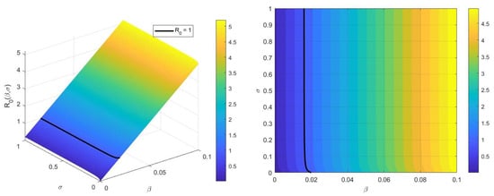
Figure 1. The effect of parameters $\sigma$ and $\beta$ on ${\mathcal{R}}_0$.

In Figure 2, we can see that augmenting the treatment rate $\alpha$ significantly reduces the quantity of ${\mathcal{R}}_0$, even when the transmission rate, $\beta$, is high. This indicates that enhancing the treatment rate, by improving access to medical care, ensuring timely diagnoses, and implementing effective therapeutic interventions, is important in limiting the spread of disease and makes it one of the most effective strategies for controlling an infectious disease.

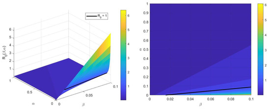
Figure 2. The effect of parameters $\alpha$ and $\beta$ on ${\mathcal{R}}_0$.

Figure 3 illustrates that the basic reproduction number ${\mathcal{R}}_0$ increases as both the transmission rate $\beta$ and parameter p rise, indicating a direct positive correlation between ${\mathcal{R}}_0$ and the pair $(\beta ,p)$. However, it can be observed that the transmission rate $\beta$ exerts a stronger influence on the value of ${\mathcal{R}}_0$ compared to p. Therefore, to reduce the quantity of ${\mathcal{R}}_0$, it should primarily focus on reducing the transmission rate, which represents a more impactful strategy for reducing the disease spread.

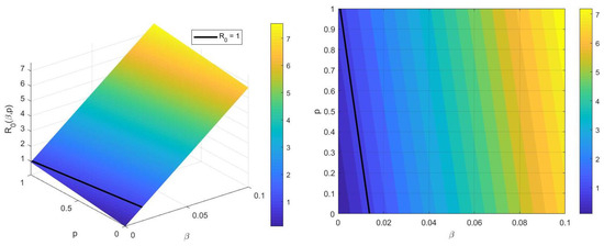
Figure 3. The effect of parameters p and $\beta$ on ${\mathcal{R}}_0$.

4.3. Evolution of the Solutions of System (52)–(54)

In this subsection, we present numerical simulations illustrating the temporal evolution of the solutions to system (52)–(54). Our aim is to show how the basic reproduction number ${\mathcal{R}}_0$ shapes the qualitative behavior of the disease. More precisely, we compare the cases ${\mathcal{R}}_0<1$ and ${\mathcal{R}}_0>1$ and analyze how these two regimes influence the long-term dynamics of the susceptible, latent, infectious, and recovered populations.

As illustrated in Figure 4, when ${\mathcal{R}}_0<1$, the disease eventually disappears from the population. Both the infectious and latent classes decline to zero, indicating that the system converges to the disease-free equilibrium $E^0$. These numerical results are in full agreement with the theoretical findings of Theorem 4, which guarantees the global asymptotic stability of $E^0$ in the regime ${\mathcal{R}}_0<1$.

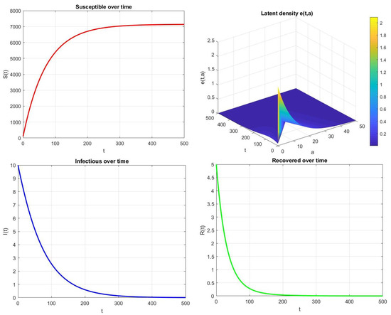
Figure 4. Time evolution of $S\left(t\right)$, $e(t,a)$, $I\left(t\right)$, and $R\left(t\right)$ for $\beta =0.15\times {10}^{-5}$, $\alpha =0.65$, $\sigma =0.015$, and ${\mathcal{R}}_0=0.4302<1$.

In contrast, when ${\mathcal{R}}_0>1$, the disease persists within the population. Figure 5 shows that the infectious and latent compartments remain strictly positive and the system approaches the endemic equilibrium $E^{*}$. This behavior is fully consistent with the theoretical predictions of Theorem 7, where the existence and global stability of the endemic equilibrium are guaranteed when ${\mathcal{R}}_0>1$.

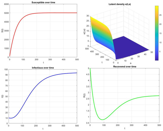
Figure 5. Time evolution of $S\left(t\right)$, $e(t,a)$, $I\left(t\right)$, and $R\left(t\right)$ for $\beta =0.15\times {10}^{-3}$, $\alpha =0.25$, $\sigma =0.075$, and ${\mathcal{R}}_0=3.4302>1$.

4.4. Dynamical Behavior of $I\left(t\right)$ Under Variation of p and $\gamma$

Figure 6–left. It is evident that increasing the value of p implies an increase in the number of infectious individuals. This occurs because a higher value of p can directly affect the relapse rate $p\sigma R\left(t\right)$, resulting in a greater number of infectious individuals. Conversely, reducing p could help to limit this relapse effect and contribute to bringing the infection under control.

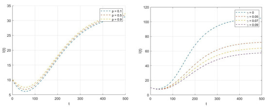
Figure 6. Dynamical behavior of $I\left(t\right)$ when p and $\gamma$ vary.

Figure 6–right. One can observe that increasing the saturation parameter $\gamma$ in the incidence function $f\left(I\right)={\displaystyle \frac{I}{1+\gamma I}}$ reduces the number of infectious individuals $I\left(t\right)$, which helps to keep the infection under control. However, when $\gamma$ takes a smaller value, the saturation effect diminishes, which allows the disease to spread strongly and aggressively through the population.

5. Conclusions

In this paper, we have investigated the global dynamics of an age-structured epidemic model that incorporates a latency period, relapse mechanisms, and nonlinear incidence effects. Our analysis showed that the basic reproduction number ${\mathcal{R}}_0$ completely governs the qualitative behavior of the system. Specifically, when ${\mathcal{R}}_0<1$, the disease eventually dies out, while for ${\mathcal{R}}_0>1$, the infection will persist and continue to spread through the population. These results underscore the decisive importance of controlling ${\mathcal{R}}_0$ as a key strategy for preventing the spread of the epidemic.

For the nonlinear incidence function $f\left(I\right)={\displaystyle \frac{\beta I}{1+\gamma I}}$, the explicit expression of ${\mathcal{R}}_0$ as given by (13) is written as follows:

$${\mathcal{R}}_0=\underset{{\mathcal{R}}_{01}}{\underbrace{{\displaystyle \frac{\beta S^0}{\mu +\alpha }}{\int }_0^{\infty }\delta \left(a\right)\zeta \left(a\right)da}}+\underset{{\mathcal{R}}_{02}}{\underbrace{{\displaystyle \frac{\alpha \sigma }{(\mu +\alpha )(\mu +\sigma )}}\left[p+(1-p){\int }_0^{\infty }\delta \left(a\right)\zeta \left(a\right)da\right]}}.$$

Interpretation of ${\mathcal{R}}_{01}$:

• $\beta S^0$: transmission rate per susceptible individual.
• ${\displaystyle \frac{1}{\mu +\alpha }}$: average duration an individual stays in the infected class.
• ${\displaystyle {\int }_0^{\infty }\delta \left(a\right)\zeta \left(a\right)da}$: probability that a newly infected individual survives the latency period and becomes infectious.

Hence, ${\mathcal{R}}_{01}$ represents the average number of secondary infections generated via the direct pathway. Interpretation of ${\mathcal{R}}_{02}$:

• ${\displaystyle \frac{\alpha }{\mu +\alpha }}$: fraction of infected individuals who recover.
• ${\displaystyle \frac{\sigma }{\mu +\sigma }}$: fraction of recovered individuals who relapse.
• The quantity

  $$p+(1-p){\int }_0^{\infty }\delta \left(a\right)\zeta \left(a\right)da$$

  represents the total probability that a recovered individual who experiences relapse will eventually become infectious again. The term p corresponds to the fraction of relapsed individuals who become immediately infectious. The remaining fraction $1-p$ re-enters the latent class, and the factor ${\int }_0^{\infty }\delta \left(a\right)\zeta \left(a\right)da$ is the probability that a latent individual survives the latency period and progresses to infectiousness. Therefore,

  $$(1-p){\int }_0^{\infty }\delta \left(a\right)\zeta \left(a\right)da$$

  gives the probability that a relapsed individual who returns to latency will eventually reach the infectious class. Summing both contributions gives the overall probability of returning to the infectious class after relapse.

Thus, ${\mathcal{R}}_{02}$ represents the average number of secondary infections generated via the relapse pathway. Consequently, ${\mathcal{R}}_0={\mathcal{R}}_{01}+{\mathcal{R}}_{02}$ accounts for all possible routes by which an initially infected individual can produce new infections in a fully susceptible population.

Based on the above brief discussion and supported by the numerical illustrations which discuss the influence of the key parameters in shaping the expression of ${\mathcal{R}}_0$, we can propose some effective control strategies that aim to keep the endemic under control:

1. Reducing the transmission rate $\beta$: Since $\beta$ has the strongest impact on the value ${\mathcal{R}}_0$, minimizing direct contact between susceptible and infectious individuals is essential. This can be achieved through classical public-health measures such as social distancing, use of protective equipment (e.g., masks), hand hygiene, and vaccination campaigns that reduce susceptibility.

2. Enhancing treatment efficacy: The treatment rate $\alpha$ plays a decisive role in shaping the epidemic dynamics. Mathematically, increasing the value of $\alpha$ effectively reduces the average of the infectious period, thereby minimizing the quantity of ${\mathcal{R}}_0$. From a public-health perspective, this emphasizes the necessity of ensuring early access to treatment, strict adherence to effective protocols, and sustained therapeutic coverage. Such measures collectively strengthen the capacity to bring ${\mathcal{R}}_0$ below unity, ensuring long-term disease control and preventing further transmission.

3. Limiting relapse and reinfection: Relapse cases in recovered individuals can act as hidden reservoirs for reinfection. Regular medical follow-up, ensuring completion of treatment protocols, and monitoring immune response (e.g., through antibody or PCR testing, depending on the pathogen) are necessary to prevent relapse and to sustain long-term immunity.

4. Adapting the incidence structure: The form of the incidence rate $f\left(I\right)$ significantly influences epidemic dynamics. From a modeling perspective, using an adaptive incidence function that reflects behavioral changes, treatment effects, or population heterogeneity can improve predictive accuracy and provide a more realistic basis for designing control policies.

In summary, the analytical and numerical results of this work indicate that it may be possible to further strengthen the model by incorporating explicit control interventions. Strategies such as vaccination, early detection of infectious individuals, improvement of treatment effectiveness, and measures aimed at reducing relapse can be represented through suitable time-dependent control functions. Embedding these controls within the model would allow for a systematic assessment of how targeted public-health actions can steer the system toward disease elimination.

References

- Castillo-Chávez, C.; Song, B. Dynamical models of tuberculosis and their applications. Math. Biosci. Eng. 2004, 1, 361–404. [Google Scholar] [CrossRef] [PubMed]
- Diekmann, O.; Heesterbeek, H.; Britton, T. Mathematical Tools for Understanding Infectious Disease Dynamics; Princeton University Press: Princeton, NJ, USA, 2013. [Google Scholar]
- Din, A.; Li, Y. Controlling heroin addiction via age-structured modeling. Adv. Differ. Equ. 2020, 2020, 521. [Google Scholar] [CrossRef]
- Foss, A.M.; Vickerman, P.T.; Chalabi, Z.; Mayaud, P.; Alary, M.; Watts, C.H. Dynamic modelling of herpes simplex virus type-2 (HSV-2) transmission: Issues in structural uncertainty. Bull. Math. Biol. 2009, 71, 720–749. [Google Scholar] [CrossRef]
- Hirsch, W.M.; Hanisch, H.; Gabriel, P. Differential equation models of some parasitic infections: Methods for the study of asymptotic behavior. Commun. Pure Appl. Math. 1985, 38, 733–753. [Google Scholar] [CrossRef]
- Kermack, W.O.; McKendrick, A.G. A contribution to the mathematical theory of epidemics. Proc. R. Soc. Lond. A 1927, 115, 700–721. [Google Scholar]
- Hu, Z.; Teng, Z.; Zhang, L. Stability and bifurcation analysis in a discrete SIR epidemic model. Math. Comput. Simul. 2014, 97, 80–93. [Google Scholar] [CrossRef]
- Tahir, H.; Khan, A.; Din, A.; Khan, A.; Zaman, G. Optimal control strategy for an age-structured SIR endemic model. Discret. Contin. Dyn. Syst. 2021, 14, 2535–2555. [Google Scholar] [CrossRef]
- Xu, R.; Ma, Z. Global stability of an SIR epidemic model with nonlinear incidence rate and time delay. Nonlinear Anal. Real World Appl. 2009, 10, 3175–3189. [Google Scholar] [CrossRef]
- Yuan, X.; Wang, F.; Xue, Y.; Liu, M. Global stability of an SIR model with differential infectivity on complex networks. Phys. A Stat. Mech. Its Appl. 2018, 499, 443–456. [Google Scholar] [CrossRef]
- Zaman, G.; Han, K.Y.; Jung, I.H. Stability analysis and optimal vaccination of an SIR epidemic model. Biosystems 2008, 93, 240–249. [Google Scholar] [CrossRef]
- Brookmeyer, R. Incubation period of infectious diseases. In Wiley StatsRef: Statistics Reference; John Wiley & Sons, Ltd.: Hoboken, NJ, USA, 2015. [Google Scholar]
- McCluskey, C.C. Global stability for an SEIR epidemiological model with varying infectivity and infinite delay. Math. Biosci. Eng. 2009, 6, 603–610. [Google Scholar] [CrossRef]
- Wang, L.; Xu, R. Global stability of an SEIR epidemic model with vaccination. Int. J. Biomath. 2016, 9, 1650082. [Google Scholar] [CrossRef]
- Nabti, A.; Kirane, M. Global dynamics of an age-structured tuberculosis model with a general nonlinear incidence rate. J. Biol. Syst. 2025, 33, 1117–1159. [Google Scholar] [CrossRef]
- Nabti, A. Dynamical analysis of an age-structured SEIR model with relapse. Z. Für Angew. Math. Und Phys. 2024, 75, 32. [Google Scholar] [CrossRef]
- Bernoussi, A. Stability analysis of an SIR epidemic model with homestead-isolation on the susceptible and infectious, immunity, relapse and general incidence rate. Int. J. Biomath. 2023, 16, 2250102. [Google Scholar] [CrossRef]
- Pradeep, B.G.S.A.; Ma, W.; Wang, W. Stability and Hopf bifurcation analysis of an SEIR model with nonlinear incidence rate and relapse. J. Stat. Manag. Syst. 2017, 20, 483–497. [Google Scholar] [CrossRef]
- Tudor, D. A deterministic model for herpes infections in human and animal populations. SIAM Rev. 1990, 32, 136–139. [Google Scholar] [CrossRef]
- Wang, J.; Pang, J.; Liu, X. Modelling diseases with relapse and nonlinear incidence: A multi-group epidemic model. J. Biol. Dyn. 2014, 8, 99–116. [Google Scholar] [CrossRef]
- Wang, J.; Shu, H. Global analysis on a class of multi-group SEIR model with latency and relapse. Math. Biosci. Eng. 2016, 13, 209–225. [Google Scholar] [CrossRef]
- Guo, Z.K.; Xiang, H.; Huo, H.F. Analysis of an age-structured tuberculosis model with treatment and relapse. J. Math. Biol. 2021, 85, 45. [Google Scholar] [CrossRef] [PubMed]
- Liu, L.; Ren, X.; Jin, Z. Threshold dynamical analysis of a class of age-structured tuberculosis model with immigration of population. Adv. Differ. Equ. 2017, 2017, 258. [Google Scholar] [CrossRef][Green Version]
- Henshaw, S.; McCluskey, C.C. Global stability of a vaccination model with immigration. Electron. J. Differ. Equ. 2015, 2015, 1–10. [Google Scholar][Green Version]
- Liu, W.M.; Levin, S.A.; Iwasa, Y. Influence of nonlinear incidence rates upon the behaviour of SIRS epidemiological models. J. Math. Biol. 1986, 23, 187–204. [Google Scholar] [CrossRef] [PubMed]
- McCluskey, C.C. Global stability for an SEI epidemiological model with continuous age-structure in the exposed and infectious classes. Math. Biosci. Eng. 2012, 9, 819–841. [Google Scholar] [CrossRef] [PubMed]
- Yang, Y.; Li, J.; Zhou, Y. Global stability of two tuberculosis models with treatment and self-cure. Rocky Mt. J. Math. 2012, 42, 1367–1386. [Google Scholar] [CrossRef]
- Barril, C.; Calsina, À; Cuadrado, S.; Ripoll, J. Reproduction number for an age of infection structured model. Math. Model. Nat. Phenom. 2021, 16, 42. [Google Scholar] [CrossRef]
- Calsina, A.; Palmada, J.M.; Ripoll, J. Optimal latent period in a bacteriophage population model structured by infection-age. Math. Model. Methods Appl. Sci. 2011, 21, 693–718. [Google Scholar] [CrossRef]
- Hethcote, H.W. Qualitative analyses of communicable disease models. Math. Biosci. 1976, 28, 335–356. [Google Scholar] [CrossRef]
- Capasso, V.; Serio, A. A generalization of the Kermack-McKendrick deterministic model. Math. Biosci. 1978, 42, 43–61. [Google Scholar] [CrossRef]
- Webb, G.F. Theory of Nonlinear Age-Dependent Population Dynamics; Marcel Dekker: New York, NY, USA, 1985. [Google Scholar]
- Iannelli, M. Mathematical Theory of Age-Structured Population Dynamics; Applied Mathematics Monographs; Comitato Nazionale per le Scienze Matematiche, Consiglio Nazionale delle Ricerche (C.N.R.): Giardini, Italy, 1995; Volume 7. [Google Scholar]
- Magal, P. Compact attractors for time-periodic age-structured population models. Electron. J. Differ. Equ. 2001, 65, 1–35. [Google Scholar]
- Smith, H.L.; Thieme, H.R. Dynamical Systems and Population Persistence. Grad. Stud. Math. 2011, 118, 405. [Google Scholar]
- Diekmann, O.; Heesterbeek, J.A.P.; Metz, J.A.J. On the definition and the computation of the basic reproduction ratio R0 in models for infectious diseases in heterogeneous populations. J. Math. Biol. 1990, 28, 365–382. [Google Scholar] [CrossRef] [PubMed]
- Hale, J.K.; Waltman, P. Persistence in infinite-dimensional systems. SIAM J. Math. Anal. 1989, 20, 388–395. [Google Scholar] [CrossRef]
- Magal, P.; Zhao, X.-Q. Global attractors and steady states for uniformly persistent dynamical systems. SIAM J. Math. Anal. 2005, 37, 251–275. [Google Scholar] [CrossRef]
- Hale, J.K. Dynamical systems and stability. J. Math. Anal. Appl. 1969, 26, 39–59. [Google Scholar] [CrossRef]
- Walker, J.A. Dynamical Systems and Evolution Equations: Theory and Applications; Plenum Press: New York, NY, USA, 1980. [Google Scholar]
- Goh, B.S. Global stability in many species systems. Am. Nat. 1977, 111, 135–142. [Google Scholar] [CrossRef]
- Sigdel, R.P.; McCluskey, C.C. Global stability for an SEI model of infectious disease with immigration. Appl. Math. Comput. 2014, 243, 684–689. [Google Scholar] [CrossRef]
- LaSalle, J.P. The Stability of Dynamical Systems; Regional Conference Series in Applied Mathematics; SIAM: Philadelphia, PA, USA, 1976. [Google Scholar]
Disclaimer/Publisher’s Note: The statements, opinions and data contained in all publications are solely those of the individual author(s) and contributor(s) and not of MDPI and/or the editor(s). MDPI and/or the editor(s) disclaim responsibility for any injury to people or property resulting from any ideas, methods, instructions or products referred to in the content. |
© 2025 by the authors. Licensee MDPI, Basel, Switzerland. This article is an open access article distributed under the terms and conditions of the Creative Commons Attribution (CC BY) license (https://creativecommons.org/licenses/by/4.0/).