Abstract
The first research attempt to dynamically optimize the CORDIC algorithm’s iteration count using artificial intelligence is presented in this paper. Conventional approaches depend on a certain number of iterations, which frequently results in extra calculations and longer processing times. Our method drastically reduces the number of iterations without compromising accuracy by using machine learning regression models to predict the near-best iteration value for a given input angle. Overall efficiency is increased as a result of reduced computational complexity along with faster execution. We optimized the hyperparameters of several models, including Random Forest, XGBoost, and Support Vector Machine (SVM) Regressor, using Grid Search and Cross-Validation. Experimental results show that the SVM Regressor performs best, with a mean absolute error of 0.045 and an R2 score of 0.998. This AI-driven dynamic iteration prediction thus offers a promising route for efficient and adaptable CORDIC implementations in real-time digital signal processing applications.
Keywords:
CORDIC Algorithm; Machine Learning Regression; Computational Mathematics; Iteration Optimization; Support Vector MAchine MSC:
68T07; 65Y10; 68W10; 94A12
1. Introduction
Given that modern digital systems continually evolve, there is a need for fast, accurate, and energy-efficient computing across numerous areas, such as signal processing, embedded systems, computer graphics, robotics, and medical devices. These systems have grown increasingly more dependent on hardware modules that can do complex calculations with little resource use and low latency. Arithmetic computation units are very important among these, and they need to be designed to find a balance between speed, accuracy, and hardware efficiency. In both industry and academia, optimizing these computational components has become a top priority, as design constraints become more strict due to the need for real-time processing and low power consumption. Recent studies confirm the importance of latency reduction and hardware efficiency in embedded and FPGA-based systems for real-time inference and signal processing tasks. For example, FPGA-accelerated architectures have demonstrated significant latency and resource savings while maintaining predictive accuracy in drone motor monitoring applications [1]; similar results have also been obtained for convolutional neural network (CNN) models designed for medical image classification, deployable on lightweight embedded platforms [2].
In this context, the Coordinate Rotation Digital Computer (CORDIC) algorithm stands out as a promising solution due to its inherent simplicity, low hardware footprint, and energy efficiency. Originally developed for real-time trigonometric computations, CORDIC has found widespread applications in digital signal processing (DSP), including in systems where conventional approaches rely on large look-up tables (LUTs) for carrier generation and transformation functions [3]. The CORDIC algorithm, introduced by Volder [4], is a well-established iterative technique used for calculating trigonometric functions through a combination of shift and addition operations, avoiding the need for multipliers. Walther extended this approach to cover a broader set of mathematical functions, including hyperbolic and exponential operations [5]. CORDIC’s efficiency and multiplier-less architecture make it particularly suitable for implementations on FPGAs, ASICs, and embedded processors [3]. Applications include image processing [6], robotics, neural networks [3], signal processing operations like FFT and DCT [7], and biomedical systems [8]. However, in systems where speed and energy efficiency are vital, the iterative nature of the algorithm still presents latency and power issues [7,9,10].
Several different types of devices use CORDIC, including digital signal processors, software-defined radios, computer graphics, robotics, and navigation systems [3,7]. It rapidly calculates trigonometric, hyperbolic, exponential, logarithmic, and linear functions, which are important for modulation/demodulation, digital filtering, phase-locked loops, coordinate transformations, and vector rotations. Because it functions well with hardware, it is very good for embedded and portable devices that have strict power and space limits [11].
Nevertheless, one of the most significant challenges with CORDIC-based systems is figuring out how many iterations are needed to get the right level of accuracy while using the least amount of hardware for computational capabilities and processing time. The standard CORDIC algorithm uses an iterative process that goes through one step at a time to get closer to the actual mathematical functions. Since it runs in a sequence, each step depends on the one before it being finished. Furthermore, the number of iterations required depends on how accurate the result should be. This dependency causes longer processing times, especially when working with data with high bit-widths. This makes latency a major problem for applications that need high precision [12], making it necessary to look into smart ways to automate and improve the process.
By developing an efficient computation technique that reduces iteration reliance while maintaining high-precision accuracy, this work addresses the intrinsic sequential delay of regular CORDIC. The suggested method cleverly reorganizes the iterative process to lower latency and increase throughput, in contrast to traditional CORDIC implementations that depend on fixed, bit-width-dependent iteration counts. Because of this, the design may achieve faster convergence with much reduced latency, which makes it ideal for real-time and high-precision applications where conventional CORDIC techniques are inadequate.
Integrating Artificial Intelligence (AI) and Machine Learning (ML) techniques into the iteration prediction process offers a promising solution. The regression models are trained to estimate the minimum and near-optimal number of iterations for a given input angle, making it possible to automate the optimization process, improving both execution speed and hardware efficiency. This research leverages Python-based ML implementations to predict the best, as well as the near-best iteration, for an angle with minimal error, and compares these predictions against conventional methods.
1.1. Motivation
The rising complexity of contemporary signal processing and communication systems demands the usage efficient algorithms that may deliver high accuracy while using a minimum number of power and hardware resources. For such devices, the CORDIC algorithm is a reasonable choice because of its hardware-friendly shift-and-add operations. However, the optimal number of iterations is usually determined using fixed, which often leads to overestimation and inefficient hardware consumption. This inefficiency is more apparent in adaptive or real-time systems, where input parameters vary significantly and a fixed iteration count cannot best balance accuracy and resource utilization. Moreover, the lack of dynamic iteration control limits the flexibility and scalability of CORDIC-based designs in evolving system needs.
The lack of techniques that intelligently calculate the optimal or near-optimum number of CORDIC iterations for each input represents the main research gap. In order to solve this, we used machine learning techniques to dynamically anticipate the best and near-best iteration counts of the CORDIC algorithm based on the input angle. This enables the creation of hardware-efficient systems that maintain accuracy without requiring unnecessary iterations.
1.2. Problem Statement
A major challenge in CORDIC-based digital signal processing systems is determining the optimal number of iterations, , required to achieve a target accuracy , while minimizing hardware complexity. Traditionally, this count is calculated using a static expression:
which tends to overestimate the necessary iterations, leading to unnecessary hardware utilization and power consumption. To overcome this limitation, we propose a machine learning-based approach that dynamically predicts the optimal iteration count as a function of the input angle :
where represents a trained regression model. The model is designed to ensure the residual angle satisfies , thus enabling a hardware-efficient CORDIC implementation with no compromise in accuracy.
1.3. Major Contributions
To overcome the drawbacks of conventional static methods, this paper suggests a novel machine learning-based method to dynamically determine the optimal and near-optimal number of iterations for the CORDIC algorithm. Our method optimizes performance and resource usage by using trained regression models to predict iteration counts based on input angles, in contrast to traditional implementations that rely on manually derived equations, which often result in overestimated iteration counts and inefficient hardware usage. Support Vector Regressor (SVR), Random Forest Regressor, and XGBoost Regressor are among the machine learning models evaluated; GridSearchCV is used for hyperparameter tuning. For the first time, the near-optimal iteration prediction is presented, which offers less hardware complexity without sacrificing accuracy. Here, machine learning models are adopted as mathematical estimators, providing a closed-form prediction of approximation quality based on the CORDIC iteration index. This transforms the empirical error behavior of CORDIC into a predictable mathematical function, aligning the work with mathematical modelling rather than general AI experimentation.
The remainder of this paper is organized as follows. Section 2 presents a review of related work and discusses existing methods for CORDIC iteration estimation. Section 3 provides a short overview of the CORDIC algorithm, including its fundamental principles, operational modes, and the traditional approach to calculating angles and determining the required number of iterations. Section 4 details the proposed methodology, which integrates machine learning models to predict both optimal and near-optimal iteration counts dynamically based on input angles. Section 5 describes the experimental framework, including dataset preparation, model training, and evaluation metrics. Section 6 presents the results and analysis, comparing the performance of different regression models and validating the hardware efficiency of the proposed approach. Finally, Section 7 concludes the paper and outlines directions for future research.
2. Related Work
The CORDIC algorithm’s efficacy has spurred numerous enhancements throughout the years to further boost its performance. Early attempts to boost throughput focused on pipelined VLSI architectures [13]. More resource-efficient real-time embedded systems were made possible throughout time by advancements like hybrid designs and improved pipeline stages [14]. Also, researchers proposed scale-free variations to omit the typical scaling factor at the conclusion of iterations, enhancing hardware efficiency by reducing superfluous multiplications [15].
Despite these improvements, a persistent limitation of many traditional CORDIC implementations is the reliance on a fixed number of iterations to ensure desired precision. This static approach often leads to over-computation, particularly for inputs that inherently demand less accuracy, thus wasting power and hardware cycles. One of the earliest methods includes the use of variable iterations tailored to the desired accuracy, which improves efficiency over fixed-iteration designs [16]. In addition, a low-latency CORDIC based on greedy algorithms has been reported to reduce average iteration counts [17]. In [18], a hybrid model is introduced that integrates the conventional CORDIC algorithm with a Variable Scaling Factor (VSF) approach. Implemented on a Cyclone IV FPGA, this design effectively reduces the number of iterations while maximizing hardware utilization. High radix and hybrid computing techniques further reduce computational cycles, and new reconfigurable CORDIC architectures support circular and hyperbolic modes while optimizing power and delay metrics [19,20]. Hardware-level improvements, such as the use of carry-select adders and canonical signed-digit representations, have also proven effective in reducing power usage and improving computation speed [21]. Also reduced number of iterations were achieved using by dedicated pre-rotation and comparison processes in [12].
Although these contributions offer significant hardware and performance gains, they typically rely on predefined logic and heuristic control mechanisms. As a result, they lack the flexibility to generalize across diverse input distributions or real-time operating conditions. No prior work has explored the use of machine learning to predict the optimal or near-optimal number of CORDIC iterations. This paper fills that gap by proposing a supervised learning framework leveraging the iteration requirements of ML models based on input angles and error tolerance. These models learn from empirical data and enable adaptive iteration control, resulting in energy-efficient and time-efficient CORDIC execution without compromising accuracy.
3. CORDIC Algorithm
The main advantage of CORDIC is its ability to carry out a variety of computations using only simple shift-and-add operations. It can handle tasks such as calculating trigonometric, hyperbolic, and logarithmic functions, performing multiplications and divisions (both real and complex), computing square roots, solving linear systems, and even operations like eigenvalue estimation, singular value decomposition, and QR factorization [22]. Because of this flexibility, CORDIC has found applications in many areas, including signal and image processing, communication systems, robotics, 3D graphics, and other scientific and technical computations.
CORDIC operates mainly in two modes: rotational and vectoring. In rotational mode, an input vector is rotated through a series of fixed micro-rotations by a target angle , resulting in a rotated vector , as shown in Figure 1. In vectoring mode, the algorithm iteratively aligns the vector with the x-axis by reducing the y-component towards zero, enabling computation of the vector’s magnitude and angle relative to the x-axis.
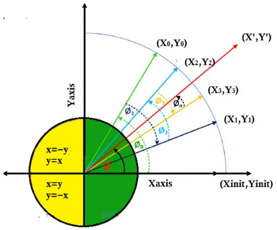
Figure 1.
Illustration of the CORDIC vector rotation principle.
CORDIC approach is popular due to the simplicity of its hardware implementation, since the same iterative algorithm may be utilized for all these applications utilizing the basic shift-add operations of the form a . Keeping the requirements and restrictions of diverse application contexts in account, the development of CORDIC algorithm and architecture has taken place for obtaining high throughput rate and decrease of hardware-complexity as well.
The iterative update equations at each iteration i are:
where is the rotation direction chosen based on the sign of the residual angle .
The total rotation angle is approximated by the sum of these micro-rotations:
Table 1 illustrates this step-by-step process, where each decision is made to iteratively bring the accumulated angle Z closer to 30°. The process continues until the residual error is minimized to an acceptable level. This is becase each micro-rotation in CORDIC is implemented using fixed shift-and-add operations that are pre-defined in hardware. The precision of the final angle depends strictly on how many of these micro-rotations are executed. If the process is stopped early, the accumulated correction sequence is incomplete, resulting in a deterministic and non-compensated residual error. As a result, CORDIC is not designed to stop based on runtime convergence criteria; instead, the iteration count is selected in advance to meet a specified precision.

Table 1.
CORDIC Iterations for Approximating a 30-Degree Rotation.
For example, to rotate by approximately 30°, the sequence of micro-rotations might be:
Since the iterative process introduces a gain, the correction factor is applied to scale the final results:
After N iterations, the vector , when scaled by , approximates . The detailed CORDIC algorithm steps are provided in Appendix A.
4. Proposed Methodology
This section describes the integrated approach for dynamically predicting the optimal and near-optimal iteration counts for the CORDIC algorithm using machine learning. The methodology involves first generating a labeled dataset by simulating the CORDIC algorithm over a range of input angles and iterations, extracting relevant features and error metrics. Subsequently, several regression models are trained on this dataset to learn the mapping from iteration features to the input angle. These models enable dynamic estimation of iteration requirements, facilitating hardware-efficient CORDIC implementations.
4.1. Simulation Based Data Generation and Labeling
The CORDIC algorithm is simulated in rotation mode for input angles ranging from 0° to 90° in increments of 5°. For each angle, iterative approximations of sine and cosine values are obtained. At each iteration i, the maximum absolute error is computed as:
where and are the approximated cosine and sine values, respectively.
Two key iterations are identified per angle: the best iteration , minimizing , and the near-best iteration inear-best, defined as the earliest iteration satisfying
with as a small tolerance threshold.
To clearly define the near-best iteration, we chose an empirical value . This value was chosen after experimenting with several thresholds and observing their effect on both the iteration count and approximation accuracy. Smaller values prevented early stopping, while larger values introduced noticeable approximation error. The selected threshold provides a balanced trade-off, enabling iteration reduction while keeping the angular error within an acceptable range for CORDIC computation.
A dataset is compiled with features including iteration count i, approximated sine , cosine , residual angle , cosine-to-sine ratio , and the maximum error . Angles from 0° to 90° were evaluated in increments of 5°, resulting in a total of 285 iteration-level datapoints. Each iteration is labeled as BEST, NEAR-BEST, or NEITHER, where BEST denotes the iteration that yields the minimum error, NEAR-BEST includes iterations satisfying (with ), and all remaining iterations are categorized as NEITHER. The distribution of samples as shown in Figure 2 with BEST–19 samples (6.67%), NEAR-BEST–19 samples (6.67%), and NEITHER–247 samples (86.67%). This feature-annotated dataset enables the machine learning model to learn the relationship between CORDIC convergence behavior and the optimal iteration count, thereby supporting accurate and hardware-efficient prediction.
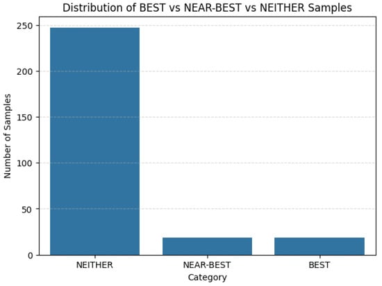
Figure 2.
Distribution of dataset samples across BEST, NEAR-BEST, and NEITHER categories.
4.2. Random Forest Regression (RF)
Random Forest regression [23,24] constructs an ensemble of decision trees . The prediction for a feature vector is the average of the outputs of all trees [23]:
This ensemble method reduces variance and overfitting, effectively modeling nonlinear dependencies. It also provides feature importance scores, aiding interpretability—valuable for understanding which iteration features influence the predicted angle most significantly [24].
4.3. Support Vector Regression (SVR)
SVR [25] aims to find a function
that approximates the target values within a margin , while minimizing complexity. The optimization problem is [25]:
subject to
where are slack variables allowing for errors beyond the -insensitive zone, and C regulates the trade-off between flatness and tolerance. Kernel functions enable SVR to handle nonlinear relationships effectively, making it suitable for complex, small, or noisy datasets.
4.4. Extreme Gradient Boosting (XGBoost)
XGBoost builds models iteratively by adding decision trees that predict the residuals of previous models. The update at iteration t is [26]:
with optimized to minimize a regularized objective balancing model accuracy and complexity. XGBoost is efficient, scalable, and powerful in capturing intricate feature interactions, commonly used for high-performance regression tasks.
These three regression models were selected for their complementary strengths in handling nonlinear data, robustness to overfitting, and balance between interpretability and computational efficiency—attributes crucial for hardware-adaptive CORDIC implementations. Hyperparameter tuning is performed via Grid Search with Cross-Validation to optimize each model’s performance. The trained models serve as predictive engines to dynamically estimate the required iteration count for any input angle, paving the way for efficient and adaptive CORDIC hardware designs.
5. Model Training and Evaluation
This section describes the process of training the regression models introduced earlier and the metrics used to evaluate their performance.
5.1. Model Training
The labeled dataset generated through CORDIC simulation is split into training (80%) and validation sets (20%) to enable robust model development and unbiased performance evaluation. To ensure generalization, each regression model—Random Forest (RF), Support Vector Regression (SVR), and Extreme Gradient Boosting (XGBoost)—undergoes hyperparameter tuning using Grid Search with 5 fold Cross-Validation (CV). In this setup, the dataset is divided into five equal parts, with the model trained on four folds and validated on the remaining one in a rotating manner. This approach ensures reliable performance estimation and prevents overfitting to any particular subset. This approach helps identify the optimal hyperparameters that minimize overfitting and improve predictive accuracy. All models are trained and hyperparameters are tuned in the Google Colab using Python 3.10 with libraries including scikit-learn, XGBoost, pandas, and NumPy, for efficient computation and faster hyperparameter optimization. A fixed random seed was applied across all models to ensure reproducibility.
Key hyperparameters tuned include:
- Random Forest: Number of trees (n_estimators), maximum tree depth (max_depth), and minimum samples per split (min_samples_split).
- SVR: Regularization parameter C, kernel type (e.g., radial basis function), and kernel-specific parameters such as gamma.
- XGBoost: Number of boosting rounds, learning rate, maximum tree depth, and subsample ratios.
After hyperparameter tuning, the best models are retrained on the full training set before evaluation on the held-out test data.
5.2. Performance Metrics
Model effectiveness is assessed using several metrics capturing different aspects of prediction accuracy:
- Mean Absolute Error (MAE) [27]: Measures average absolute difference between predicted and true angles:where and denote the true and predicted angle values, respectively.
- Coefficient of Determination ( Score) [28]: Indicates the proportion of variance in the dependent variable predictable from the features:where is the mean of true values.
- Accuracy within : The percentage of predictions within one degree of the true angle, measuring tolerance to minor deviations.
The Mean Absolute Error (MAE) was used as the main criterion for selecting the best hyperparameters, as it directly measures how closely the predicted iteration values match the ground truth. To give another perspective on the total accuracy of the regression, the coefficient of determination () is also reported. The final chosen hyperparameters are shown in Table 2. This process was systematically applied to SVR, Random Forest, and XGBoost models. We report the best hyperparameters and give a brief explanation of how they were chosen. A maximum depth of 10 provided the optimum balance between bias and variance for the Random Forest model; shallower configurations decreased prediction accuracy, while deeper trees tended to overfit during cross-validation. The choice of 100 estimators similarly emerged as a practical compromise, as larger values did not yield meaningful performance gains but increased training time. For the SVR model, the parameters and were identified through systematic exploration within the Grid Search space: smaller C values led to underfitting, while larger values increased sensitivity to noise. In XGBoost, the combination of a depth of 3 and a learning rate of 0.1 produced the most stable generalization performance across the validation folds. These observations are based on empirical behaviour during cross-validation and are now included to clarify the reasoning behind the selected hyperparameters.
Table 2.
Best Hyperparameters Selected by Grid Search CV.
These metrics together provide a comprehensive evaluation of model performance in terms of precision, generalization, and practical usability for hardware iteration prediction. Also, to keep the results consistent and comparable, the same random seed was used throughout the entire process—covering data shuffling, splitting, initialization, and training. This ensured that any differences in performance were due to the models themselves and not random fluctuations.
For visual analysis, tools such as scatter plots of predicted versus true angles, box plots illustrating error distributions, and histograms showing error counts are employed. These visualizations help in intuitively understanding the spread, skewness, and frequency of prediction errors, offering deeper insights beyond numerical metrics.
6. Results and Analysis
A thorough analysis of the three regression models—SVR, Random Forest, and XGBoost—using a variety of statistical indicators and reliability metrics based on confidence intervals is shown in Table 3. SVR consistently outperforms the other models in terms of prediction, with the lowest MAE (0.28158) and the highest coefficient of determination (R2 = 0.99924). The SVR model maintains consistent and trustworthy predictions across various resampling distributions, as further demonstrated by the tight 95% confidence intervals for both MAE and R2.
Table 3.
Comprehensive performance comparison of RF, SVR, and XGBoost regressors with advanced error metrics.
Additionally, the Random Forest model achieves competitive R2 of 0.99891 and reasonable MAE values. Its error distribution appears to be more variable, nevertheless, as indicated by the larger confidence intervals as compared to SVR. Among the three, the XGBoost model performs the worst, as seen by greater MAE and MSE values, a lower R2, and somewhat lower angular precision. XGBoost’s sensitivity to outliers is indicated by its greater MaxAE, which further restricts its applicability for this regression job. All things considered, the findings unequivocally show that SVR is the most efficient and trustworthy model for estimating the ideal CORDIC iteration angle. Its capacity to minimize both average and worst-case prediction errors is demonstrated by its outstanding performance across all error metrics, including MAE, MSE, MAPE, MaxAE, and accuracy-based measures.
Figure 3 illustrates the predicted versus true angle values for three regression models—Random Forest Regressor, Support Vector Regressor (SVR), and XGBoost Regressor—each evaluated for their ability to accurately estimate angular values. In all three subplots, the green dashed line represents the ideal case where predicted angles perfectly align with the true values, while the red dots mark the actual predictions made by each model. The degree to which the red points align with the diagonal line serves as a visual indicator of the performance of each model.
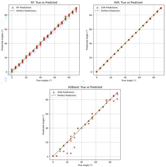
Figure 3.
True vs. Predicted angles for Random Forest (RF), Support Vector Regressor (SVR), and XGBoost models.
Among the three, the SVR model demonstrates near-perfect performance. Its predictions are almost entirely aligned with the ideal line, exhibiting minimal to no visible deviation. Quantitatively, SVR achieves a Mean Absolute Error (MAE) of just 0.0581, an R2 score of 1.0000, and a rounded accuracy of 98.25%. Notably, its prediction accuracy within a tolerance of ±1° reaches 100%, confirming the model’s remarkable precision. This performance reflects SVR’s capacity to capture fine-grained variations in angular values across the range of test data. The Random Forest Regressor, while not as flawless as SVR, also exhibits strong predictive performance. The corresponding subplot shows predicted values closely clustered around the ideal line, although with slightly more dispersion, particularly at the boundaries.
In contrast, the XGBoost Regressor displays a broader spread of predictions around the diagonal, especially in mid-range angles, indicating a lower degree of precision. This observation is supported by its quantitative metrics, which include a notably higher MAE of 1.45 and a lower R2 score of 0.9822. The rounded accuracy and accuracy within ±1° are also considerably lower at 56.14% and 59.65%, respectively. One potential reason for XGBoost’s underperformance could be its sensitivity to noise or small fluctuations in data when the signal-to-noise ratio is low, particularly in regression tasks involving fine-grained, continuous outputs such as angle estimation. In such contexts, the ensemble of weak learners may struggle to capture subtle patterns without overfitting or introducing variance in mid-range predictions.
Statistical Test: Using the error values from both approaches for each assessed angle, a paired t-test was conducted to see whether the SVR model’s reduction in prediction error is statistically significant. For every angle, the absolute CORDIC error and the associated SVR error were considered as paired observations. The test then computed the mean difference between the two error sets and evaluated whether this improvement was larger than what could occur by chance. A p-value below 0.05 indicates that the SVR’s improvement over CORDIC is statistically significant.
The prediction error distributions for the Random Forest, SVR, and XGBoost models are shown in Figure 4. The SVR model shows a symmetric distribution that is tightly clustered around zero, with most errors falling within ±0.1°. This minimal spread validates SVR’s stability and accuracy in angle estimation by demonstrating its high precision and low variance. The model’s remarkable performance, as proved by its low MAE and perfect R2 score, is further supported by the sharp peak at zero and the absence of significant outliers.
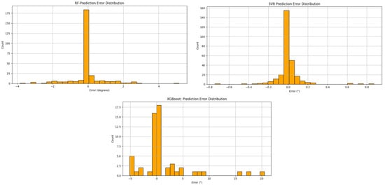
Figure 4.
Error distribution histograms for Random Forest, SVR, and XGBoost models. The histograms show how prediction errors are distributed for each model, with SVR displaying the narrowest and most centered distribution.
With errors primarily falling within the range of ±4°, the Random Forest model, in contrast, displays a wider but still centrally concentrated error distribution. The greater dispersion indicates sporadic errors, especially at the prediction boundaries, even though it retains a noticeable peak at zero. The XGBoost model, however, presents a much wider and more irregular error distribution, with predictions spreading from approximately −10° to +20°. This high variance and the presence of multiple peaks imply instability and reduced predictive reliability. These visual patterns align with the model’s poorer performance metrics, including the highest MAE and the lowest accuracy within ±1°, highlighting XGBoost’s limited effectiveness in this fine-grained regression task as shown in Figure 5.
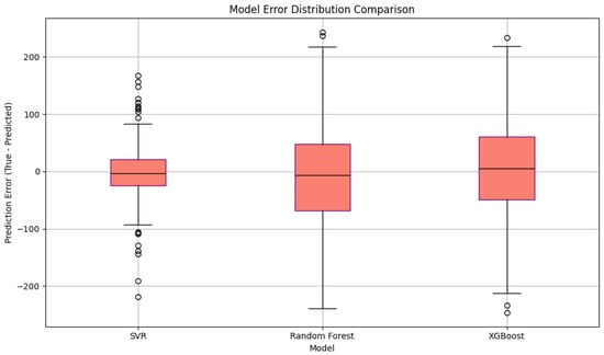
Figure 5.
Prediction error boxplot comparison across SVR, Random Forest, and XGBoost models. The y-axis indicates the prediction error (True—Predicted).
The learning curves for SVR, Random Forest, and XGBoost models are plotted against increasing training samples in Figure 6. SVR demonstrates rapid convergence with minimal generalization gap, achieving near-perfect R2 scores on both training and validation sets early on, indicating excellent generalization and minimal overfitting. With a slight but constant difference between training and validation scores, Random Forest exhibits a steady upward trend, indicating moderate bias but a great overall potential for generalization. On the other hand, XGBoost exhibits poor generalization and overfitting due to its high training accuracy and notable divergence from validation scores. T he plateau in validation performance despite increasing training data suggests limited benefit from additional data for XGBoost in this regression scenario.
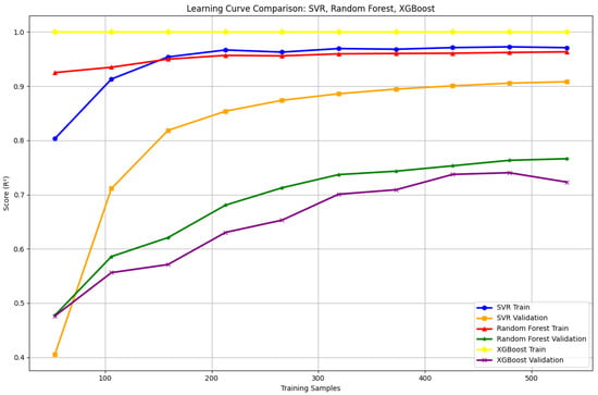
Figure 6.
Learning curve comparison of SVR, Random Forest, and XGBoost models showing training and validation R2 scores across varying training set sizes.
The proposed near-best iteration prediction strategy reduces the number of CORDIC iterations compared to the conventional fixed-iteration method, as shown in Figure 7. The blue curve depicts the percentage reduction in iterations for each input angle, measured as the relative difference between the fixed and predicted near-best iterations. The greatest angular error (in degrees) related to the predicted near-best iterations is displayed by the red dashed curve. As can be observed, the suggested approach exhibits both excellent accuracy and computing efficiency by drastically reducing the number of iterations across all angles while maintaining low angular errors. The efficacy of the AI-driven iteration prediction is quantitatively validated by this visualization.
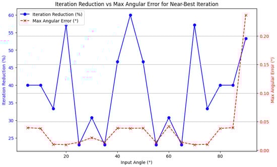
Figure 7.
Iteration reduction (%) and maximum angular error (°) for each input angle using the near-best iteration approach.
A comparison of the Support Vector Regression (SVR) model and the traditional CORDIC approach for angle estimation on optimal iteration counts is shown in Table 4. To guarantee accuracy, a set number of repeats is employed for every angle in conventional CORDIC implementations. Nevertheless, this uniform technique leads to more hardware requirements and redundant computations. On the other hand, the SVR model maintains excellent accuracy while using fewer resources by predicting a near-optimal number of iterations tailored to each input angle.
Table 4.
Comparison Between CORDIC and SVR Predicted Iterations for Angle Estimation.
As illustrated in Table 4, SVR predicted iteration counts are often lower than the fixed CORDIC count, with negligible absolute error (usually below 0.05°). For example, for 30°, CORDIC uses 13 iterations, while SVR predicts just 9, yielding a close estimate with only 0.042° error. Even at higher angles like 90°, the SVR model approximates well with fewer iterations. In this study, we fixed the iteration count to 15 for dataset creation. However, our SVR model effectively identifies the near-best iteration that minimizes angular error. This enables significant reductions in computation time and hardware complexity. For instance, although CORDIC approximates 30° accurately by the 9th iteration, it continues through all 15 steps. Using SVR prediction (iteration 9), we achieve nearly identical accuracy with fewer operations, demonstrating the efficiency of the model for real-time applications with limited resources.
To assess the impact of our approach on computational efficiency, we compared the performance of the three regression models—SVR, Random Forest, and XGBoost—using prediction accuracy, angular error, training time, and inference time as key metrics. As summarized in With the lowest iteration prediction error (MAE of 0.0581), the smallest angular variation (0.00044°), and the fastest inference time (92 ns), the SVR model consistently performs better than the others, as shown in Table 5. Accurately predicting the necessary number of iterations immediately contributes to a reduction in computational costs because the CORDIC algorithm’s runtime grows in proportion to the number of iterations. For instance, for an input angle such as 30°, the conventional fixed-iteration strategy executes all 15 steps, even though convergence is effectively reached after the 9th iteration. The total number of operations drops by about 40% when the SVR model predicts this optimal point, which lowers latency and reduces internal transitions during processing. Without impacting system time, the prediction overhead is negligible and can be incorporated as a lightweight control step. The superior performance of the SVR model can be attributed to the characteristics of the dataset and the nature of the underlying mapping. The prediction challenge is highly suited for kernel-based regression since the features produced from the CORDIC process show an almost monotonic trend and fluctuate smoothly with the input angle. While tree-based models like Random Forest and XGBoost produce piecewise-constant functions that might cause discontinuities and are more likely to overfit in low-dimensional, noise-sensitive environments, the RBF kernel in SVR successfully preserves these continuous nonlinear relationships. As a result, SVR attains reduced prediction error and more robust generalization over the whole range of input angles. These results demonstrate that the proposed dynamic iteration approach is extremely appropriate for real-time and hardware-constrained implementations since it maintains numerical precision while drastically reducing processing effort.
Table 5.
Comparison of Machine Learning Models for Dynamic CORDIC Iteration Prediction.
7. Conclusions
The first study to use machine learning for this purpose is this paper, which presents a novel AI-based method to dynamically forecast the near-optimal iteration count for the CORDIC algorithm. Our approach efficiently lowers the number of iterations needed by using regression models, specifically the Support Vector Machine, which results in a reduction in processing time and computational complexity while preserving exceptional precision. The experimental results confirm that dynamic iteration prediction enhances the efficiency of CORDIC computations, making it a promising solution for real-time and resource-constrained digital signal processing applications. Future work may explore hardware implementations and extend the model to other CORDIC variants.
Author Contributions
Conceptualization, A.M., C.R. and R.S.; Methodology, R.S.; Software, L.C.R.; Investigation, C.R., V.F. and R.S.; Resources, L.C.R.; Data Curation, L.C.R. and V.F.; Supervision, A.M. and C.R.; Paper Writing, C.R., R.S. and L.C.R.; Paper Writing—Critical Revision, V.F. and A.M.; Project Administration, C.R.; Funds Acquisition, A.M. and V.F. All authors have read and agreed to the published version of the manuscript.
Funding
This research was funded by Committee of Science of the Ministry of Science and Higher Education of the Republic of Kazakhstan, Project SmartEdu: grant number BR28713531, and it was funded by Department for Cohesion Policy and South, Italian Government, Project PARIDE grant number E87G23000120001.
Institutional Review Board Statement
Ethical approval, informed consent, and adherence to institutional or licensing regulations are not applicable.
Data Availability Statement
The original contributions presented in this study are included in the article. Further inquiries can be directed to the corresponding author.
Conflicts of Interest
The authors declare no potential conflict of interests.
Nomenclature
| Symbol | Description |
| Optimal number of iterations | |
| Residual Angle for optimal iterations | |
| Target Accuracy | |
| Trained machine learning model | |
| Input Angle | |
| Correction factor | |
| C | Regularization parameter |
| R2 | Coeffecient of Determination |
Appendix A. CORDIC Algorithm Step-by-Step
The CORDIC algorithm iteratively approximates trigonometric functions using shift-and-add operations. The steps for the rotation mode are summarized below:
- Initialize the input vector:where is the scaling constant.
- For each iteration :
- (a)
- Determine rotation direction:
- (b)
- Update vector components:
- (c)
- Compute current errors (optional for dataset creation):
- After all iterations, and approximate and , respectively.
References
- Priya, S.S.; Sanjana, P.S.; Yanamala, R.M.R.; Amar Raj, R.D.; Pallakonda, A.; Napoli, C.; Randieri, C. Flight-Safe Inference: SVD-Compressed LSTM Acceleration for Real-Time UAV Engine Monitoring Using Custom FPGA Hardware Architecture. Drones 2025, 9, 494. [Google Scholar] [CrossRef]
- Randieri, C.; Perrotta, A.; Puglisi, A.; Grazia Bocci, M.; Napoli, C. CNN-Based Framework for Classifying COVID-19, Pneumonia, and Normal Chest X-Rays. Big Data Cogn. Comput. 2025, 9, 186. [Google Scholar] [CrossRef]
- Węgrzyn, M.; Voytusik, S.; Gavkalova, N. FPGA-based Low Latency Square Root CORDIC Algorithm. J. Telecommun. Inf. Technol. 2025, 1, 21–29. [Google Scholar] [CrossRef]
- Volder, J.E. The CORDIC trigonometric computing technique. IRE Trans. Electron. Comput. 1959, EC-8, 330–334. [Google Scholar] [CrossRef]
- Walther, J.S. A unified algorithm for elementary functions. In Proceedings of the Spring Joint Computer Conference, Alantic, NJ, USA, 18–20 May 1971; pp. 379–385. [Google Scholar]
- Vucha, M.; Siridhara, A. Cordic Architecture for Discrete Cosine Transform. In Proceedings of the 2021 6th International Conference on Communication and Electronics Systems (ICCES), Coimbatre, India, 8–10 July 2021; IEEE: Piscataway, NJ, USA, 2021; pp. 229–232. [Google Scholar]
- Changela, A.; Zaveri, M.; Lakhlani, A. ASIC implementation of high performance radix-8 CORDIC algorithm. In Proceedings of the 2018 International Conference on Advances in Computing, Communications and Informatics (ICACCI), Bangalore, India, 19–22 September 2018; IEEE: Piscataway, NJ, USA, 2018; pp. 699–705. [Google Scholar]
- Jain, N.; Mishra, B. CORDIC on a configurable serial architecture for biomedical signal processing applications. In Proceedings of the 2015 19th International Symposium on VLSI Design and Test, Ahmedabad, India, 26–29 June 2015; IEEE: Piscataway, NJ, USA, 2015; pp. 1–6. [Google Scholar]
- Verma, S.K.; Pullakandam, M.; Yanamala, R.M.R. Pipelined CORDIC Architecture Based DDFS Design and Implementation. In Proceedings of the 2023 IEEE 20th India Council International Conference (INDICON), Hyderabad, India, 14–17 December 2023; IEEE: Piscataway, NJ, USA, 2023; pp. 1440–1445. [Google Scholar]
- Bhukya, S.; Inguva, S.C. Design and Implementation of CORDIC algorithm using Integrated Adder and Subtractor. In Proceedings of the 2021 6th International Conference for Convergence in Technology (I2CT), Maharashtra, India, 2–4 April 2021; IEEE: Piscataway, NJ, USA, 2021; pp. 1–5. [Google Scholar]
- Asok, N.; Nikhil, V.; Manoj, C.; Sunder, K.; Reddy, V.; Rajeswari, P. Implementation of low power CORDIC algorithm. J. Eng. Appl. Sci. 2018, 13, 842–847. [Google Scholar]
- Li, K.; Fang, H.; Ma, Z.; Yu, F.; Zhang, B.; Xing, Q. A Low-Latency CORDIC Algorithm Based on Pre-Rotation and Its Application on Computation of Arctangent Function. Electronics 2024, 13, 2338. [Google Scholar] [CrossRef]
- Rai, S.; Dwivedi, C.; Srivastava, R. Pipelined cordic architecture and its implementation on Simulink. In Proceedings of the 2017 3rd International Conference on Computational Intelligence & Communication Technology (CICT), Ghaziabad, India, 9–10 February 2017; IEEE: Piscataway, NJ, USA, 2017; pp. 1–10. [Google Scholar]
- Chakraborty, A.; Banerjee, A. Cordic-based high-speed vlsi architecture of transform model estimation for real-time imaging. IEEE Trans. Very Large Scale Integr. (VLSI) Syst. 2020, 29, 215–226. [Google Scholar] [CrossRef]
- Paramasivam, C.; Chauhan, S.S.; Meena, V.; Sreejagathi, A.; Hasini, B.; Kishore, K.; Vamsikrishna, T.; Anantasai, M.D.; Didi, A. Enhanced Performance of New Scaling-free CORDIC for Memory-based Fast Fourier Transform Architecture. IEEE Access 2025, 13, 19828–19844. [Google Scholar] [CrossRef]
- Mane, M.; Patil, D.; Sutaone, M.S.; Sadalage, A. Implementation of DCT using variable iterations CORDIC algorithm on FPGA. In Proceedings of the 2014 First International Conference on Computational Systems and Communications (ICCSC), Trivandrum, India, 17–18 December 2014; IEEE: Piscataway, NJ, USA, 2014; pp. 379–383. [Google Scholar]
- Hou, N.; Wang, M.; Zou, X.; Liu, M. A Low Latency Floating Point CORDIC Algorithm for Sin/Cosine Function. In Proceedings of the 2019 IEEE 4th International Conference on Signal and Image Processing (ICSIP), Wuxi, China, 19–21 July 2019; IEEE: Piscataway, NJ, USA, 2019; pp. 751–755. [Google Scholar]
- Xue, Y.; Ma, Z. Design and implementation of an efficient modified CORDIC algorithm. In Proceedings of the 2019 IEEE 4th International Conference on Signal and Image Processing (ICSIP), Wuxi, China, 19–21 July 2019; IEEE: Piscataway, NJ, USA, 2019; pp. 480–484. [Google Scholar]
- Feng, Z.; Chang, H.; Zhang, H.; Li, A.; Xing, L. Design and Implementation of High-speed and High-precision CORDIC Algorithm. In Proceedings of the 2024 6th International Conference on Frontier Technologies of Information and Computer (ICFTIC), Qingdao, China, 13–15 December 2024; IEEE: Piscataway, NJ, USA, 2024; pp. 1050–1056. [Google Scholar]
- Bai, N.; Qu, R.; Xu, Y.; Wang, Y.; Chen, X.; Li, L. Low-iteration hybrid computing CORDIC architecture. Microelectron. J. 2025, 156, 106481. [Google Scholar] [CrossRef]
- Inguva, S.C.; Seventline, J. FPGA based Implementation of Low power CORDIC architecture. In Proceedings of the 2019 International Conference on Intelligent Sustainable Systems (ICISS), Palladam, India, 21–22 February 2019; IEEE: Piscataway, NJ, USA, 2019; pp. 389–395. [Google Scholar]
- Meher, P.K.; Valls, J.; Juang, T.B.; Sridharan, K.; Maharatna, K. 50 years of CORDIC: Algorithms, architectures, and applications. IEEE Trans. Circuits Syst. I Regul. Pap. 2009, 56, 1893–1907. [Google Scholar] [CrossRef]
- Breiman, L. Random forests. Mach. Learn. 2001, 45, 5–32. [Google Scholar] [CrossRef]
- Schonlau, M.; Zou, R.Y. The random forest algorithm for statistical learning. Stata J. 2020, 20, 3–29. [Google Scholar] [CrossRef]
- Xue, H.; Yang, Q.; Chen, S. SVM: Support vector machines. In The Top Ten Algorithms in Data Mining; Chapman and Hall/CRC: Boca Raton, FL, USA, 2009; pp. 51–74. [Google Scholar]
- Nalluri, M.; Pentela, M.; Eluri, N.R. A scalable tree boosting system: XG boost. Int. J. Res. Stud. Sci. Eng. Technol. 2020, 7, 36–51. [Google Scholar]
- Willmott, C.J.; Matsuura, K. Advantages of the mean absolute error (MAE) over the root mean square error (RMSE) in assessing average model performance. Clim. Res. 2005, 30, 79–82. [Google Scholar] [CrossRef]
- Chicco, D.; Warrens, M.J.; Jurman, G. The coefficient of determination R-squared is more informative than SMAPE, MAE, MAPE, MSE and RMSE in regression analysis evaluation. PeerJ Comput. Sci. 2021, 7, e623. [Google Scholar] [CrossRef] [PubMed]


Disclaimer/Publisher’s Note: The statements, opinions and data contained in all publications are solely those of the individual author(s) and contributor(s) and not of MDPI and/or the editor(s). MDPI and/or the editor(s) disclaim responsibility for any injury to people or property resulting from any ideas, methods, instructions or products referred to in the content. |
© 2025 by the authors. Licensee MDPI, Basel, Switzerland. This article is an open access article distributed under the terms and conditions of the Creative Commons Attribution (CC BY) license (https://creativecommons.org/licenses/by/4.0/).