Null Lagrangians and Gauge Functions in Physics: Applications and Recent Developments

Abstract

The Lagrangian formalism has provided a powerful and elegant framework for obtaining governing equations for classical and quantum systems. It is based on the concept of action, which involves Lagrangians, whose a priori knowledge is required. There are different methods to obtain Lagrangians for given equations of motion, and a brief review of these methods is presented. However, the main purpose of this review paper is to describe the so-called null Lagrangians and their gauge functions, and discuss their physical applications. The paper also reviews some recent results, which demonstrate that gauge functions play the most fundamental roles in classical dynamics as they can be used to predict the future states of dynamical systems, without solving the equations of motion, as well as to construct their Lagrangians.

1. Introduction

The astounding progress of modern physics in discovering and understanding the fundamental laws of Nature that govern the structure and evolution of the Universe, and its matter and energy, has been possible because of the used powerful mathematical-empirical approach. In this approach, physical theories are formulated using the language of mathematics and their predictions are verified experimentally. An important role in formulating theories of modern physics has been played by the calculus of variations, which was originally developed by Euler [1] and Lagrange [2], who used the Principle of Least Action that determines a path that corresponds to the action reaching its minimum or maximum values [2].

Generalization of this principle was performed by Hamilton [3], who introduced the Principle of Stationary Action (PSA), also known as the Hamilton Principle, and showed that the PSA could be used to find a path along which the value of the action was stationary; with the latter corresponding to either minimum or maximum or saddle point. The action was defined as an integral over a scalar function called Lagrangian that originally represented the difference between the kinetic and potential energies of a system from its initial to final time. It was shown that the value of the action was different for every possible path connecting the initial and final points. Then, the PSA was used to determine the path that corresponds to the stationary action [4,5,6].

The PSA was originally developed for classical dynamical systems, and it was demonstrated that the principle gave identical formulation of classical mechanics as the Newton second law of dynamics [2,3,4,5,6,7]. However, the principle was also used to formulate other theories of physics, especially those involving classical and quantum fields (e.g., [8] and references therein). This makes the PSA one of the most powerful and elegant principles of modern physics.

Typically, Lagrangians are divided into two families, namely, standard and non-standard Lagrangians. Despite the fact that the mathematical forms of standard and non-standard Lagrangians are different, and so is the physical meaning of the terms that constitute them, the Lagrangians give the same equations of motion when substituted into the Euler–Lagrange (E-L) equation. Both standard and non-standard Lagrangians have been commonly used to obtain different equations of motion in applied mathematics and classical and quantum physics [4,5,6,7,8].

There are no general methods to obtain standard and non-standard Lagrangians from first principles. However, for some dynamical systems, Lagrangians can be constructed by accounting either for invariance of laws of physics, or invariance of a physical system under consideration, or mathematical structure (linear or nonlinear, driven or undriven, damped or undamped) of its equation of motion (e.g., [4,5,6,7]). Historically, most equations of modern physics were established first and only then were their Lagrangians found, often by guessing (e.g., [8]). This paper gives a brief review of both standard and non-standard Lagrangians, and methods developed to find such Lagrangians for given equations of motion.

There is another family of Lagrangians that is significantly different from the families of standard and non-standard Lagrangians. These are the so-called null (or trivial) Lagrangians (NLs), which identically satisfy the E-L equation, and they are easy to construct as the total derivative of any scalar, smooth and differentiable function becomes an NL [9]; such a function is called a gauge function, and the name is used throughout this paper. In mathematics, NLs of different forms were constructed and used in Cartan and Lepage forms, which are differential forms associated with NLs, in studying symmetries of different Lagrangians, and in Carathéodory’s theory of fields and extremals and integral invariants (e.g., [9,10,11,12,13,14] and references therein).

Since null Lagrangians do not give any equation of motion when substituted into the E-L equation, their previous applications in physics were very limited; an exception was elasticity, where they were used to represent the energy density function of materials [15,16,17]. In the last several years, some interesting applications of NLs and their gauge functions (GFs) in different dynamical systems were reported, and they are described in this paper. Moreover, the paper also reviews the most recent results that demonstrate fundamental roles played by NLs and GFs in classical dynamics, and their relationships to non-standard Lagrangians. Thus, the main objective of this paper is to review null Lagrangians and gauge functions, demonstrate their applications to a variety of dynamical systems, and describe the most recent developments in this new and exciting field of research.

This review paper is organized as follows: principle of stationary action and Lagrangian formalism are described in Section 2; an overview of Helmholtz conditions and standard Lagrangians is given in Section 3; non-standard Lagrangians and methods to construct them are presented in Section 4; an overview of null Lagrangians and gauge functions and their physical applications can be found in Section 5; recent developments are described and discussed in Section 6; fundamental roles of gauge functions in classical dynamics are discussed in Section 7; and concluding remarks and perspectives are given in Section 8.

2. Principle of Stationary Action and Lagrangian Formalism

Let $S[x\left(t\right),t_i,t_f]$ be the action, which is a functional that represents a physical system, with t being time, and $t_i$ and $t_f$ being the initial and final values of time., respectively. The action is defined by the following integral

$$S[x\left(t\right),t_i,t_f]={\int }_{t_i}^{t_f}L[\dot{x}\left(t\right),x\left(t\right),t]dt,$$

(1)

where $L(\dot{x}\left(t\right),x\left(t\right),t)$ is a scalar function called Lagrangian, and $\dot{x}$ is derivative of x with respect to t. Using this definition, the Hamilton principle can be expressed mathematically as $\delta S=0$, where $\delta$ is the variation of action, also known as the functional (or Fréchet) derivative of $S$ with respect to the function $x\left(t\right)$. The necessary condition that the Hamilton principle is satisfied is given by the Euler–Lagrange (E-L) equation, whose operator $\widehat{EL}$ is given by

$$\widehat{EL}\equiv {\displaystyle \frac{d}{dt}}\left({\displaystyle \frac{\partial }{\partial \dot{x}}}\right)-{\displaystyle \frac{\partial }{\partial x}}.$$

(2)

Then, the E-L equation can be written as $\widehat{EL}\left[L(\dot{x},x,t)\right]=0$. This equation guarantees that the action is stationary, which means that it has either a minimum or maximum or saddle point [4,5,6].

The mathematical basis for this approach is a smooth configuration manifold $\mathcal{Q}$ with a tangent bundle $T\mathcal{Q}$. Then, the Lagrangian $L(\dot{x},x)$ is defined as a $C^{\infty }$ map from $T\mathcal{Q}$ to the real line $\mathbf{R}$, or $L:T\mathcal{Q}\to \mathbf{R}$ [6]. Similarly, the explicit dependence of this Lagrangian on time can be expressed as $L:T\mathcal{Q}\times \mathbf{R}\to \mathbf{R}$, which gives $L(\dot{x},x,t)$. A priori knowledge of the Lagrangian for a given dynamical system allows using the E-L equation to derive the equation of motion for this system. The process of deriving equations of motion for known Lagrangians is called Lagrangian formalism.

In mathematics, the basis for the Lagrange formalism is the jet-bundle theory in which Lagrangians are defined and studied [9,10,11,12,13,14]. Let T and X be differentiable manifolds of dimensions $N+n$ and n, respectively, and let $\pi :T\to X$ be a fiber bundle structure, with $\pi$ being the canonical projection of the fibration. Typically, in classical field theories, X represents a spacetime manifold, and the fibers of T are expressed in terms of field variables. Let $J_m^r\left(T\right)\to X$ be the r-th jet bundle, with $r\in IN$. An r-th order jet with source $x\in X$ and target $t\in T$ form a class of smooth maps $\xi :X\to T$ with $t=\xi \left(x\right)$, and having partial derivatives in x up to order r, and the r-th order jet bundle extension is given by $J_n^r\left(T\right)\equiv \cup J_{x,t}^r$. Then, an ordinary differential equation (ODE) of order q is called locally variational if and only if there exists a local real function L, called a Lagrangian, constrained by the condition $q\le r$. Such Lagrangians are not unique as other Lagrangians may also exist.

3. Methods to Construct Standard Lagrangians

3.1. Helmholtz Conditions for Conservative Systems

For conservative dynamical systems, the Helmholtz conditions (HCs) are necessary and sufficient for the existence of Lagrangians [18,19]. The procedure of finding Lagrangians for given equations of motion is called the inverse (or Helmholtz) problem of calculus of variations [20,21,22,23]. Different methods are required to solve the Helmholtz problem for standard and non-standard Lagrangians, and one of the goals of this paper is to describe such methods and apply them to selected dynamical systems for which the equations of motion are already known.

Let $F_i(x_j^{\prime \prime },x_j^{\prime },x_j,t)=0$ be a set of n ODEs, with $i=1,2,...,n$ and $j=1,2,...,n$; then, the HC are

$${\displaystyle \frac{\partial F_i}{\partial x_j^{\prime \prime }}}={\displaystyle \frac{\partial F_j}{\partial x_i^{\prime \prime }}},$$

(3)

$${\displaystyle \frac{\partial F_i}{\partial x_j}}-{\displaystyle \frac{\partial F_j}{\partial x_i}}={\displaystyle \frac{1}{2}}{\displaystyle \frac{d}{dt}}\left({\displaystyle \frac{\partial F_i}{\partial x_j^{\prime }}}-{\displaystyle \frac{\partial F_j}{\partial x_i^{\prime }}}\right),$$

(4)

and

$${\displaystyle \frac{\partial F_i}{\partial x_j^{\prime }}}+{\displaystyle \frac{\partial F_j}{\partial x_i^{\prime }}}=2{\displaystyle \frac{d}{dt}}\left({\displaystyle \frac{\partial F_j}{\partial x_i^{\prime \prime }}}\right).$$

(5)

It is easy to verify that for a conservative dynamical system with its equation of motion given by $\ddot{x}+{\omega }_o^{2}x=0$, where x is a displacement, $\ddot{x}$ is the second derivative of x with respect to time t, and ${\omega }_o$ = const is the system’s natural frequency, the HCs are satisfied. This means that system’s Lagrangian $L_{so}(\dot{x},x)$ exists and that it can be constructed from the difference of the kinetic and potential energy of this system, which gives $L_{so}(\dot{x},x)=({\dot{x}}^2-{\omega }_o^2{x}^2)/2$. The Lagrangian is called the standard Lagrangian (SL), and its substitution into the E-L equation gives the equation of motion for an undamped and undriven linear oscillator.

The SLs can be obtained for given equations of motion directly from the Helmholtz conditions. Other methods include guessing, or using the invariance of a physical system under consideration, or the structure of its already known equation of motion. There are also other methods to obtain SLs and the basic idea that underlies these methods is generalization of the already known SL, which expresses the difference between the kinetic and potential energy terms, to one-dimensional dynamical systems described by either linear or nonlinear second-order ODEs with variable coefficients [24,25,26,27]).

It must also be pointed out that the HCs can be generalized to include the multiplier tensor, which for one-dimensional dynamical systems considered above become a scalar function that plays a role of integrating factor. An equation of motion with a dissipative term, which according to the HCs is a non-Lagrangian system, can be multiplied by this function and the E-L equation of some Lagrangian is obtained. In other words, the method allows finding Lagrangians for dissipative systems. The method can be generalized to multi-dimensional systems and then the multiplier becomes a symmetric, non-singular second-rank tensor, or multiplier matrix as originally named by Douglas [20].

3.2. Other Standard Lagrangians

For the following equation of motion with its nonlinear damping term, $\ddot{x}+b\left(x\right){\dot{x}}^2+c\left(x\right)g\left(x\right)=0$, where $b\left(x\right)$, $c\left(x\right)$ and $g\left(x\right)$ are continuous and differentiable functions, a method to find its Lagrangian was developed in [24], and this method requires performing an integral transform that introduces a scalar function, which removes the nonlinear damping term. Then, the resulting Lagrangian is

$$L_{bc}(\dot{x},x)={\displaystyle \frac{1}{2}}{\dot{x}}^2{e}^{2I_b\left(x\right)}-{\int }^{x}c\left(\tilde{x}\right)g\left(\tilde{x}\right)e^{2I_b\left(\tilde{x}\right)}d\tilde{x},$$

(6)

where

$$I_b\left(x\right)={\int }^{x}b\left(\tilde{x}\right)d\tilde{x}.$$

(7)

This Lagrangian is identified as an SL because the kinetic and potential energy-like terms can be recognized and they do not depend explicitly on time t. In case, $b\left(x\right)=b_o$ = const, $c\left(x\right)=c_o$ = const, and $g\left(x\right)=x$, the SL reduces to $L_s(\dot{x},x)=[{\dot{x}}^2-c_o(2b_{o}x-1)/4b_o^2]e^{2b_{o}x}$.

The above results were further generalized to ODEs of the form $\widehat{D}y\left(x\right)=0$, where $\widehat{D}=d^2/d{x}^2+B\left(x\right)d/dx+C\left(x\right)$ is a linear operator with $B\left(x\right)$ and $C\left(x\right)$ being smooth functions with at least two continuous derivatives., whose solutions can be special functions of mathematical physics [28,29]. It is seen that by making appropriate changes of variables in Equations (6) and (7), the SLs for all the special function ODEs can be obtained [30], and their relationship to Lie groups can be demonstrated [31]. However, if the coefficients in equations of motion are explicit functions of t, the resulting Lagrangians depend explicitly on time $L_{ns}(\dot{x},x,t)$, and they are called non-standard Lagrangians (NSLs); these NSLs form a large class of Lagrangians obtained by different methods that are briefly described below.

4. Non-Standard Lagrangians and Methods to Construct Them

4.1. Definition and Properties of Non-Standard Lagrangians

As defined above, the SLs are characterized by the presence of the kinetic and potential energy-like terms, and by showing no explicit dependence on time. Therefore, the SLs must have specific forms with the energy-like terms to be easily identified; an example of such an SL is given by Equation (6). The fact that there are other Lagrangians, in which these energy-like terms are not easily distinguishable, has been known since Arnold [7] introduced the so-called ‘non-natural’ Lagrangians that have become later known as non-standard Lagrangians (NSLs).

These Lagrangians cannot be constructed simply from the difference of the kinetic and potential energy, because they typically have more complicated dependence on the dynamical variables such as x and $\dot{x}$ even for systems with only one degree of freedom. Nevertheless, such NSLs can be constructed, but it is required that they give the same equations of motion as the SLs. Since the NSLs are usually explicit functions of time, they are time-dependent Lagrangians even for equations of motion whose coefficients are time-independent or constant.

In general, the NSLs can be obtained for dynamical systems that are either linear or nonlinear, damped or undamped, and driven or undriven, including all possible combinations. Based on this definition, it is obvious that some NSLs can be derived for equations of motion that may not satisfy the HCs, specifically the third one. The existence of the NSLs that violate the HCs demonstrates the limitation of these conditions.

In the following, different methods to construct NSLs are presented and applications of these NSLs to various dynamical systems are discussed. The main point is that for a given equation of motion, different NSLs can be found and that each one of them is significantly different from the SL for this equation; nevertheless, when substituted into the E-L equation, all these different Lagrangians give the same original equation of motion.

4.2. Caldirola–Kanai Lagrangian and Other Non-Standard Lagrangians

Let us consider a damped linear oscillator described by the equation of motion $\ddot{x}+{\alpha }_o\dot{x}+{\omega }_o^{2}x=0$, where ${\alpha }_o$ = const is a damping coefficient. It is easy to verify that the third HC is not satisfied. In other words, according to Helmholtz [18,19], there is no Lagrangian for this system, which is also consistent with the Bauer theorem [32]. A possible solution was proposed by Bateman [33], who suggested to consider a system of coupled oscillators with the damping term having different signs in their equations of motion, and demonstrated that such a coupled (two-dimensional) system has its Lagrangian.

A different solution was presented by Caldirola [34] and Kanai [35], who showed that the equation of motion is obtained by using the following Lagrangian:

$$L_{CK}(\dot{x},x,t)={\displaystyle \frac{1}{2}}\left[{\dot{x}}^2-{\omega }_o^2{x}^2\right]e^{{\alpha }_{o}t}\equiv L_{so}(\dot{x},x)e^{{\alpha }_{o}t}.$$

(8)

which is now known as the Caldirola–Kanai (CK) Lagrangian [34,35,36]; a method to derive $L_{CK}(\dot{x},x,t)$ is presented in [37]. It is seen that the CK Lagrangian contains the SL for a harmonic oscillator multiplied by an exponential function of time, which makes the Lagrangian time-dependent. As a result, the CK Lagrangian is typically considered to be an NSL.

Substitution of $L_{CK}(\dot{x},x,t)$ into the E-L equation gives the following equation of motion $[\ddot{x}+{\alpha }_o\dot{x}+{\omega }_o^{2}x]e^{{\alpha }_{o}t}=0$, which does obey the third condition of the HCs because of the presence of the exponential function in the equation. Nevertheless, for such systems, the total energy is not conserved; however, the energy function is conserved. Detailed studies presented in [37] showed that the energy function, which depends on the canonical momentum, remains constant in time, but the total energy that depends on the system’s linear momentum is not constant in time. Differences between the canonical and linear momenta of classical dynamical systems is discussed in [38], which also points out some conceptual errors made in previous work (e.g., [39,40]) dealing with the CK Lagrangian.

Non-standard Lagrangians of different forms were found for dissipative dynamical systems using a method based on fractional order calculus, which was developed by Rewe [41,42]. It was also shown that different NSLs are obtained when the Rayleigh extension of Lagrangian formalism is applied to systems that have non-potential (dissipative) forces [5,6,43]; the extension was recently used to determine both SLs [27] and NSLs [44] for several population dynamics models. A canonical approach to dynamical systems with friction that strongly depends on velocity was developed and its applications were presented and discussed in [45].

4.3. Direct Method and Its Non-Standard Lagrangians

The so-called reciprocal Lagrangians, which are inverses of standard-like Lagrangians, were introduced and studied in [46,47], and they are now known as non-standard Lagrangians. Generalization of such NSLs were performed in [25,26], and for the equation of motion $\ddot{x}+a\left(t\right){\dot{x}}^2+b\left(t\right)\dot{x}+c\left(t\right)x=0$, where $a\left(t\right)$, $b\left(t\right)$ and $c\left(t\right)$ are at least twice differentiable functions, the following NSL was considered:

$$L_{ns1}(\dot{x},x,t)={\displaystyle \frac{1}{f\left(t\right)\dot{x}+g\left(t\right)x+h\left(t\right)}},$$

(9)

with $f\left(t\right)$, $g\left(t\right)$ and $h\left(t\right)$ being at least twice differentiable scalar functions of the independent variable t. To determine these functions, $L_{ns1}(\dot{x},x,t)$ is substituted into the E-L equation, and the equation of motion, whose coefficients are given in terms of the functions, is obtained. Then, comparison of this equation of motion to the original one allows expressing the functions in terms of the coefficients $a\left(t\right)$, $b\left(t\right)$ and $c\left(t\right)$. The method is called ‘direct’ because the form of the Lagrangian is given in advance and because of the procedure of finding its arbitrary functions.

However, for the equation of motion $\ddot{x}+\alpha \left(x\right){\dot{x}}^2+\beta \left(x\right)\dot{x}+\gamma \left(x\right)x=0$, where $\alpha \left(x\right)$, $\beta \left(x\right)$ and $\gamma \left(x\right)$ are at least twice differentiable functions, the generalized NSL [25,26,48] was considered in the following form:

$$L_{ns2}(\dot{x},x)={\displaystyle \frac{1}{F\left(x\right)\dot{x}+G\left(x\right)x+H\left(x\right)}},$$

(10)

where $F\left(x\right)$, $G\left(x\right)$ and $H\left(x\right)$ are at least twice differentiable scalar functions of the dependent variable x, and to be determined from the same procedure as described above; further generalization of this NSL was proposed in [49]. Despite the fact that $L_{ns2}(\dot{x},x)$ does not depend explicitly on time, this Lagrangian is called non-standard because of its form, which neither resembles kinetic nor potential energy-like terms.

The conditions for the existence of $L_{ns1}(\dot{x},x,t)$ and $L_{ns2}(\dot{x},x)$ were investigated in [48], and it was shown that the procedure of finding the arbitrary functions requires solving nonlinear (Riccati-type) equations (see [31], and its Proposition 6). Applications of the NSLs to a variety of dynamical systems were presented and discussed in many papers (e.g., [25,26,31,48,50]). The NSLs were also obtained for the equations whose solutions are special functions of mathematical physics [30] as well as for several population dynamics models [44,51].

4.4. Jacobi Last Multiplier Method and Its Non-Standard Lagrangians

The Jacobi last multiplier originally introduced by Jacobi in 1842 [52] has become a powerful method to derive NSLs as demonstrated by Nucci and coworkers in a series of published papers (e.g., [53,54,55,56,57], and references therein). Let $\ddot{x}=\mathsf{\Phi }(\dot{x},x,t)$ be a second-order ODE, and $L(\dot{x},x,t)$ be a Lagrangian, then, the Jacobi last multiplier and the Lagrangian are related by

$$M(\dot{x},x,t)={\displaystyle \frac{{\partial }^{2}L(\dot{x},x,t)}{\partial {\dot{x}}^2}},$$

(11)

where $M_i(\dot{x},x,t)$ is the Jacobi last multiplier that satisfies

$${\displaystyle \frac{d}{dt}}\left(\log M(\dot{x},x,t)\right)+{\displaystyle \frac{\partial \mathsf{\Phi }(\dot{x},x,t)}{\partial \dot{x}}}=0.$$

(12)

Once $M(\dot{x},x,t)$ is known, then the Lagrangian is obtained from

$$L(\dot{x},x,t)=\int \left(\int M(\dot{x},x,t)d\dot{x}\right)d\dot{x}+f_1(x,t)\dot{x}+f_2(x,t),$$

(13)

with

$$f_1(x,t)={\displaystyle \frac{\partial G(x,t)}{\partial x}},\mathrm{and}{f}_2(x,t)={\displaystyle \frac{\partial G(x,t)}{\partial t}}+f_3(x,t),$$

(14)

where $f_3(x,t)$ must satisfy $\ddot{x}=\mathsf{\Phi }(\dot{x},x,t)$, and $G(x,t)$ is an arbitrary function to be determined [55,56].

The Jacobi last multiplier method was successfully used to obtain NSLs for a variety of physical systems described by linear and nonlinear ODEs with damping and driving forces [53,54,55,56,57]. Applications of the method to some population dynamics models [58,59] demonstrated that the resulting NSLs were identical to those found in an ad hoc manner in earlier work [60,61]. The method was also used by other authors to find NSLs for different dynamical systems and for some mathematical (Riccati) equations [62,63,64] as well as to explore nonlocal and Hojman symmetries, and Hamel’s formalism [65,66,67].

4.5. El-Nabulsi Non-Standard Lagrangians and Their Applications

The so-called El-Nabulsi Lagrangians are important NSLs that are constructed by taking either exponential, or logarithmic, or different power-laws of SLs for given dynamical systems. These Lagrangians and a broad range of their applications were presented by El-Nabulsi in different papers (e.g., [68,69,70,71,72], and references therein). In the following, the exponential and power-law NSLs are briefly described; note that El-Nabulsi Lagrangians are classified as NSLs because of their forms and in agreement with their original classification by the author (e.g., [70,71,72]).

For the exponential NSL, the action given by Equation (1) becomes

$$S(\dot{x},x)=\int e^{L_s(\dot{x},x)}dt,$$

(15)

where $x=x\left(t\right)$. Then, the PSA gives $\delta S=0$ and the following E-L equation:

$${\displaystyle \frac{d}{dt}}\left({\displaystyle \frac{\partial L_s}{\partial \dot{x}}}\right)-{\displaystyle \frac{\partial L_s}{\partial x}}+\left[\dot{x}{\displaystyle \frac{\partial L_s}{\partial x}}+\ddot{x}{\displaystyle \frac{\partial L_s}{\partial \dot{x}}}\right]\left({\displaystyle \frac{\partial L_s}{\partial \dot{x}}}\right)=0.$$

(16)

For the power-law $(1+\gamma )$ NSL, the action becomes

$$S(\dot{x},x)=\int L_s^{1+\gamma }(\dot{x},x)dt,$$

(17)

where $\gamma$ is any real number, and $\delta S=0$ gives

$${\displaystyle \frac{d}{dt}}\left({\displaystyle \frac{\partial L_s^{1+\gamma }}{\partial \dot{x}}}\right)-{\displaystyle \frac{\partial L_s^{1+\gamma }}{\partial x}}+\left[\dot{x}{\displaystyle \frac{\partial L_s^{1+\gamma }}{\partial x}}+\ddot{x}{\displaystyle \frac{\partial L_s^{1+\gamma }}{\partial \dot{x}}}\right]\left({\displaystyle \frac{\partial L_s^{1+\gamma }}{\partial \dot{x}}}\right)=0.$$

(18)

The main advantage of using the El-Nabulsi Lagrangians, which are constructed from already known SLs, is that they may show different dynamical characteristics of a considered system, like its hidden symmetries not exposed by their SLs, and may allow finding different conserved and non-conserved quantities. Other physical implications of these NSLs can be seen in their many applications that range from ordinary dynamical systems, quantum mechanics, molecular physics, and solar physics, to different aspects of cosmology [68,69,70,71,72,73,74,75,76,77,78]; this shows that the El-Nabulsi Lagrangians can be used to study many different physical problems.

4.6. Other Non-Standard Lagrangians

An interesting form of a Lagrangian was found in [79], who discovered a unique nonlinear oscillator, whose all bounded periodic motions are simple harmonic. The resulting Lagrangian contains SL-like terms divided by another term that makes it an NSL; this special oscillator and its NSL were studied by others [80,81].

A very different NSL was constructed for a simple harmonic oscillator in [82]. This NSL contains the kinetic and potential energy-like terms, it does not depend explicitly on time, and yet it is classified as an NSL because of its unusual form:

$$L_{ns}(\dot{x},x)={\displaystyle \frac{\dot{x}}{\omega x}}\arcsin \left({\displaystyle \frac{\dot{x}}{\omega x}}\right)-{\displaystyle \frac{1}{2}}\ln ({\dot{x}}^2+\omega x^2).$$

(19)

This NSL was later used to construct another NSL for the Liénard type nonlinear oscillator [83]; see also [84,85] and other NSLs for this oscillator. The basic idea presented in [83] is that the NSL found for a linear oscillator can be used to construct a new NSL for a nonlinear oscillator, and that the latter can be reduced to the former when the nonlinearity is neglected.

Most results presented in this section and the previous sections concern one-dimensional dynamical systems. However, there were also studies of two- and multiple-degrees-of-freedom systems, and the conditions for the existence of NSLs for such systems were established (e.g., [86,87]). This is an interesting extension of the well-established results obtained for simple one-dimensional systems to systems with many degrees of freedom.

Non-standard Lagrangians of different forms were also used in quantum field theories, specifically, to reformulate the Yang–Mills field theory [88], set up a cutoff limit on the Higgs field [89], and introduce a fermion field from the non-uniqueness principle [90].

5. Null Lagrangians and Gauge Functions and Their Applications

5.1. Definition and Main Characteristics

All Lagrangians that belong to the families of standard and non-standard Lagrangians give equations of motion when substituted into the E-L equation. Null Lagrangians, $L_n$, are different as they identically yield zero when the E-L operator is acting $\widehat{EL}\left[L_n(\dot{x},x,t)\right]=0$, which means that there is no resulting equation fo motion [9]. Another property of the E-L operator is that $\widehat{EL}[d\mathsf{\Phi }(x,t)/dt]=0$, where $\mathsf{\Phi }(x,t)$ is any scalar and differential function, and $d\mathsf{\Phi }(x,t)/dt$ is the total derivative of this function [9]. This shows that

$$L_n(\dot{x},x,t)={\displaystyle \frac{d\mathsf{\Phi }(x,t)}{dt}}=\left({\displaystyle \frac{\partial \mathsf{\Phi }}{\partial \dot{x}}}\right)\ddot{x}+\left({\displaystyle \frac{\partial \mathsf{\Phi }}{\partial x}}\right)\dot{x}+{\displaystyle \frac{\partial \mathsf{\Phi }}{\partial t}},$$

(20)

and that it is easy to generate NLs as there are many scalar and differentiable functions in mathematics; the function $\mathsf{\Phi }(x,t)$ is often called the gauge function, and this name will be used throughout this paper.

The two main properties of NLs described above clearly indicate that the NLs can be added to either SLs or NSLs; there will be no changes in the forms of the resulting equations of motion. Thus, from a physical point of view, one may consider NLs to be of no interest for any physical applications. It is the main goal of this review paper to demonstrate that this view is incorrect and that NLs do play important roles in physics (e.g., [15,16,17,91,92,93]) as is shown below.

5.2. Applications in Mathematics to Forms and Fields

Studies of NLs in mathematics date back to the early 1960s [93] and have continued throughout the following two decades (e.g., [94,95,96,97,98,99]). As already briefly mentioned in the Introduction, the NLs have also been an active current area of research in mathematics (e.g., [9,10,11,12,13,14]). Specifically, the studies have involved structures and constructions of these Lagrangians [9,13,99], their geometric formulations [11], Cartan and Lepage forms and symmetries of Lagrangians [10,14,95,98], and their roles in Carathéodory’s theory of fields of extremals and integral invariants [12,97,100]. In these studies, different forms of NLs were considered, including higher-order NLs [96,100], and their specific applications to different mathematical problems were presented and discussed.

The problem of identification and classification of all NLs remains not fully solved yet either in the framework of either dynamics of classical particles or classical fields [101]. First and higher order NLs in classical field theories have been studied and their descriptions were given, and it was shown that any higher order NL can be expressed as the horizontal component of the exterior derivative of a projectable form [102]. A complete analysis of the second-order NLs in classical field theory was performed by using the jet-bundle formalism [103], and it was shown that the dependence of NLs on higher order derivatives results from the horizontalisation operation as demonstrated in [102].

5.3. Liquid Crystals, Elasticity and Elastostatics

The first known application of null Lagrangians to physics goes back to the early 1960s [104]. In this work the results presented in [93] were used to identify a nilpotent energy in liquid crystals as an NL. The next application happened more than two decades later and it involved nematic elastomers, which are materials exhibiting both elastic and liquid crystalline properties [15]. In this paper, a continuum-mechanical theory for nematic elastomers was developed and the theory combined the classical liquid theory developed in [93] with nonlinear elasticity. The NLs were used to represent any energy density of these materials that does not contribute to the equilibrium equation for a given energy function [15]. To identify these special energy densities, it is important to determine all NLs that can be defined for the theories. The NLs for the theory of liquid crystals were already obtained in [93]. However, all NLs for nonlinear elasticity were derived and classified in [16], who based their work on [99].

In more recent work [17], the range of admissible boundary conditions was explored by adding the NLs to variational problems. The obtained results were applied to elasticity, where establishing specific boundary conditions is important to properly address issues related to the existence of solutions and surface potentials, and in elastostatics, which deals with bars, beams, and plates.

5.4. Newton’s First Law and Its Lagrangian

The law of inertia for one-dimensional (along x) motion of a body in an inertial frame is given by $\ddot{x}\left(t\right)=0$, and the standard Lagrangian for this equation is $L_s\left(\dot{x}\right)=C_o{\left[\dot{x}\left(t\right)\right]}^2/2$, where $C_o$ is a constant to be determined. It is well-known that the law of inertia is Galilean invariant [5,6] and that its SL is not [4,7]. Galilean invariance requires that a given equation of motion and its Lagrangian are invariant with respect to all transformations (translations in space and time, rotations and boosts) that form the Galilean group of the metric [105].

In order to fix the Galilean invariance of $L_s\left[\dot{x}\left(t\right)\right]$, the following null Lagrangian was constructed [106]:

$$L_n(\dot{x},x,t)=C_1\dot{x}x+C_2(\dot{x}t+x)+C_3\dot{x}+C_4,$$

(21)

where $C_1$, $C_2$, $C_3$ and $C_4$ are arbitrary constants. The obtained $L_n[\dot{x}\left(t\right),x\left(t\right),t]$ is the most general NL that can be constructed by taking the lowest orders of the dynamical variable. The gauge function (GF) that corresponds to the constructed NL is given by

$${\mathsf{\Phi }}_n(x,t)={\displaystyle \frac{1}{2}}{C}_1{x}^2+C_{2}xt+C_{3}x+C_{4}t.$$

(22)

Then, the total derivative of the this GF can be added to the SL, and the following Lagrangian is obtained:

$$L_t(\dot{x},x,t)=L_s\left(\dot{x}\right)+{\displaystyle \frac{d{\mathsf{\Phi }}_n(x,t)}{dt}}.$$

(23)

This addition does not change the resulting equation of motion but now Galilean invariance of $L_t(\dot{x},x,t)$ can be investigated [106].

Let $(x,t)$ and $(x^{\prime },t^{\prime })$ be inertial frames that move with respect to each other with velocity $v_0$ = const in the x-direction. Then the Galilean boosts relating these two systems are $x^{\prime }=x-v_{0}t$ and $t^{\prime }=t$. Applying these transformations to $L_t(\dot{x},x,t)$, it can be shown that

$$L_s\left[\dot{x}\left(t\right)\right]+{\displaystyle \frac{d{\mathsf{\Phi }}_n(x,t)}{dt}}\to L_s^{\prime }\left[{\dot{x}}^{\prime }\left(t\right)\right]+{\displaystyle \frac{d{\mathsf{\Phi }}_n^{\prime }(x^{\prime },t^{\prime })}{d{t}^{\prime }}},$$

(24)

which means that both SLs and both total derivatives of GFs are Galilean invariant. The presented results demonstrate that an SL, which is not Galilean invariant, can only be made Galilean invariant if this SL is supplemented by a null Lagrangian that must also be Galilean invariant [106].

5.5. Standard and Non-Standard Null Lagrangians and Gauge Functions

The simplest from of null Lagrangian is $L_n\left(\dot{x}\right)=c\dot{x}$ [9], which is the lower order than typical dependence of the standard Lagrangian $L_s\left(\dot{x}\right)={\dot{x}}^2/2$; in this paper, the NLs of this form will be called standard NLs. Based on the above definition, the gauge function (GF) that corresponds to this NL is given by $\mathsf{\Phi }(x,t)=c_{1}xt$ [9]. This shows that the NLs can be constructed by specifying GFs and then using them to calculate the resulting NLs [91].

The gauge function $\mathsf{\Phi }(x,t)$ can be generalized [91] by writing

$${\mathsf{\Phi }}_{g1}(x,t)=\sum _{m=1}\sum _{n=1}{C}_{m,n}{x}^m{t}^n,$$

(25)

where $C_{m,n}$ are arbitrary real constants, and m and n are positive integers; note that each term must have the same dimension as ${\mathsf{\Phi }}_{g1}(x,t)$, which requires that the constants have different dimensions and that their physical meaning may be different. The obtained GF gives the following higher-order NL

$$L_{ng1}(\dot{x},x,t)=\sum _{m=1}\sum _{n=1}{C}_{m,n}\left[m\dot{x}t+nx\right]x^{m-1}{t}^{n-1}.$$

(26)

Then, ${\mathsf{\Phi }}_{g1}(x,t)$ can be generalized [91] by replacing the independent variable t by a differentiable function $f_m\left(t\right)$, and the result is

$${\mathsf{\Phi }}_{g2}(x,t)=\sum _{m=1}{c}_m{x}^m{f}_m\left(t\right),$$

(27)

where $c_m$ are real constants with m being positive integers. The resulting NL can be written as

$$L_{ng2}(\dot{x},x,t)=\sum _{m=1}\left[m{f}_m\left(t\right)\dot{x}\left(t\right)+{\dot{f}}_m\left(t\right)x\right]c_m{x}^{m-1}.$$

(28)

Finally, ${\mathsf{\Phi }}_{g2}(x,t)$ can be further generalized [91] by replacing the dependent variable x by a differentiable function $g_n\left(x\right)$. This gives

$${\mathsf{\Phi }}_{g3}(x,t)=\sum _{m=1}\sum _{n=1}{c}_{m,n}{f}_m\left(t\right)g_n\left(x\right),$$

(29)

and its corresponding NL is given by

$$L_{ng3}(\dot{x},x,t)=\sum _{m=1}\sum _{n=1}{c}_{m,n}\left[{\dot{f}}_m\left(t\right)g_n\left(x\right)+\dot{x}\left(t\right)f_m\left(t\right)g_n^{\prime }\left(x\right)\right].$$

(30)

Note that each term in the above GFs and NLs are partial gauge functions and partial null Lagrangians, and that based on their forms, they are considered to be standard GFs and standard NLs to distinguish them from the so-called non-standard GFs and non-standard NLs, which are of different forms as is now demonstrated.

The first non-standard null Lagrangian was introduced in [92] in the following form

$$L_{nsn1}(\dot{x},x)={\displaystyle \frac{a_1\dot{x}}{a_{2}x+a_3}},$$

(31)

where $a_1$, $a_2$ and $a_3$ are constants. The gauge function of this non-standard NL is given by

$${\mathsf{\Phi }}_{nsn1}\left(x\right)={\displaystyle \frac{a_1}{a_2}}ln|a_{2}x+a_3|.$$

(32)

The differences between standard and non-standard NLs and GFs can be seen by comparing $L_{nsn1}(\dot{x},x)$ and ${\mathsf{\Phi }}_{nsn1}\left(x\right)$ to those given by Equations (25)–(30).

Then, it was suggested [92] that $L_{nsn1}(\dot{x},x)$ can be generalized by replacing the constants $a_1$, $a_2$ and $a_3$ in ${\mathsf{\Phi }}_{nsn1}\left(x\right)$ by at least twice differentiable functions $h_1\left(t\right)$, $h_2\left(t\right)$ and $h_3\left(t\right)$, respectively. The resulting GF is

$${\mathsf{\Phi }}_{nsgn}\left(x\right)={\displaystyle \frac{h_1\left(t\right)}{h_2\left(t\right)}}ln|h_2\left(t\right)x+h_4\left(t\right)|,$$

(33)

which gives the following non-standard null Lagrangian

$$L_{nsgn}(\dot{x},x,t)={\displaystyle \frac{h_1\left(t\right)[h_2\left(t\right)\dot{x}+{\dot{h}}_2\left(t\right)x]+{\dot{h}}_4\left(t\right)}{h_2\left(t\right)[h_2\left(t\right)x+h_4\left(t\right)}}+\left[{\displaystyle \frac{{\dot{h}}_1\left(t\right)}{h_2\left(t\right)}}-{\displaystyle \frac{h_1\left(t\right){\dot{h}}_2\left(t\right)}{h_2^2\left(t\right)}}\right]ln|h_2\left(t\right)x+h_4\left(t\right)|,$$

(34)

that satisfies $\widehat{EL}\left\{L_{nsgn}(\dot{x},x,t)\right\}=0$. The above GF and NL were derived based on the condition that the power of the dependent variable in the resulting non-standard NL is either the same as, or lower than, that displayed in the NSL given by Equation (9). In general, the functions $h_1\left(t\right)$, $h_2\left(t\right)$ and $h_3\left(t\right)$ are arbitrary; however, some mathematical [92] or physical (see Section 5.6) constraints can be imposed to restrict these functions.

The main purpose of constructing the generalized GFs and their corresponding NLs is to be able to account for different forces and nonlinearities in dynamical systems. Thus, in the following, it is demonstrated how the derived generalized GFs and NLs can be utilized to introduce different forces and nonlinearities to otherwise undriven and linear oscillators. It must be noted that the constructed standard GFs and NLs give different periodic forces and some types of nonlinearities. However, the derived non-standard GF and NL give a dissipative force or Rayleigh’s function [5,6]. Detailed derivations and the resulting forces and nonlinearities are now presented.

5.6. Forces and Nonlinearities in Classical Dynamics

The above results demonstrate that addition of a time-dependent NL to the SL for the law of inertia makes the resulting Lagrangian Galilean invariant. However, the explicit dependence on time implies that the energy is not conserved and that the energy function given by

$$E(\dot{x},x,t)=\dot{x}{\displaystyle \frac{\partial L(\dot{x},x,t)}{\partial \dot{x}}}-L(\dot{x},x,t),$$

(35)

must be calculated [5,6]. Introducing $L(\dot{x},x)=L_s(\dot{x},x)+L_n(\dot{x},x,t)$, the energy function becomes

$$E(\dot{x},x,t)=\dot{x}{\displaystyle \frac{\partial (L_s+L_n)}{\partial \dot{x}}}-(L_s+L_n)=E_s(\dot{x},x)+E_n(x,t).$$

(36)

where $E_s(\dot{x},x)$ represents the total energy of the system, and

$$E_n(x,t)=-{\displaystyle \frac{\partial {\mathsf{\Phi }}_n}{\partial t}},$$

(37)

which shows that the gauge function ${\mathsf{\Phi }}_n$ must be an explicit function of t to guarantee that $E_n(x,t)\ne 0$. There are GFs that do not depend explicitly on t, such as ${\mathsf{\Phi }}_{n1}=C_1{x}^2/2$ or ${\mathsf{\Phi }}_{n3}=C_{3}x$ (see Equation (22), or Equation (32)), with $E_n\left(x\right)=0$ for these GFs.

An interesting result is that the obtained $E_n(x,t)$ itself is not an NL, which means that it can be directly added to, or subtracted from, a given SL to obtain the following new total Lagrangian

$$L_{tot}(\dot{x},x,t)=L_s(\dot{x},x)\pm E_n(x,t).$$

(38)

Substitution of $L_{tot}(\dot{x},x,t)$ into the E-L equation gives

$${\displaystyle \frac{d}{dt}}\left({\displaystyle \frac{\partial L_s}{\partial \dot{x}}}\right)-{\displaystyle \frac{\partial L_s}{\partial x}}=\pm {\displaystyle \frac{\partial E_n}{\partial x}},$$

(39)

and the term on the RHS of this equation can be identified as a force that would appear in the equation of motion, and it is given by

$$F\left(t\right)=\pm {\displaystyle \frac{\partial E_n}{\partial x}}=\pm {\displaystyle \frac{\partial }{\partial x}}\left({\displaystyle \frac{\partial {\mathsf{\Phi }}_n}{\partial t}}\right).$$

(40)

The presence of a forcing term on the RHS of the E-L equation is a well-known phenomenon in classical dynamics, where typically the term collects all forces not arising from potentials [5]; for frictional forces that are proportional to velocities, the forcing term is called Rayleigh’s dissipation force [5,6]. However, here the procedure of introducing $F\left(t\right)$ allows converting the equation of motion for an undriven oscillator into a driven one [107,108].

The procedure shows that different GFs give different forces [91]. Using the general GFs given by Equations (25), (27) and (29), the following forces are obtained:

$$F_{g1}(x,t)=\sum _{m=1}\sum _{n=1}mn{C}_{m,n}{x}^{m-1}{t}^{n-1},$$

(41)

$$F_{g2}(x,t)=\sum _{m=1}m{\dot{f}}_m\left(t\right)c_m{x}^{m-1}.$$

(42)

and

$$F_{g3}(x,t)=\sum _{m=1}{c}_{m,n}{\dot{f}}_m\left(t\right)g_n^{\prime }\left(x\right),$$

(43)

where $g_n^{\prime }\left(x\right)$ is the derivative of $g_n\left(x\right)$ with respect to x. The force $F_{g3}(x,t)$ is the most general that can be obtained under these conditions, and it is given as the infinite sum of all differentiable functions. The GFs required to introduce forces into otherwise undriven dynamical systems are given in Table 1, which was originally presented in [91].

Table 1. Forces in selected dynamical systems and their gauge functions (after [91]).

Dynamical Systems	Force $\mathit{F}\left(\mathit{t}\right)$	Gauge Function $\mathbf{\Phi }(\mathit{x},\mathit{t})={\mathbf{\Phi }}_1(\mathit{x},\mathit{t})+{\mathbf{\Phi }}_2(\mathit{x},\mathit{t})$
Driven	$F\left(t\right)=F_{0}cost$	${\mathsf{\Phi }}_1(x,t)=x{F}_{0}sint$
oscillators		${\mathsf{\Phi }}_2(x,t)=0$
	$F\left(t\right)=F_0{cos}^{2}t$	${\mathsf{\Phi }}_1(x,t)={\displaystyle \frac{1}{2}}xt{F}_0$
	$={\displaystyle \frac{1}{2}}{F}_0(1+cos2t)$	${\mathsf{\Phi }}_2(x,t)={\displaystyle \frac{1}{4}}x{F}_{0}sin2t$
	$F\left(t\right)=F_0{cos}^{3}t$	${\mathsf{\Phi }}_1(x,t)={\displaystyle \frac{3}{4}}x{F}_{0}sint$
	$={\displaystyle \frac{1}{4}}{F}_0(3cost+cos3t)$	${\mathsf{\Phi }}_2(x,t)={\displaystyle \frac{1}{12}}x{F}_{0}sin3t$
	$F\left(t\right)=F_0{e}^{it}$	${\mathsf{\Phi }}_1(x,t)=-ix{F}_0{e}^{it}$
		${\mathsf{\Phi }}_2(x,t)=0$
	$F\left(t\right)=F_{1}cost$	${\mathsf{\Phi }}_1(x,t)=x{F}_{1}sint$
	$+F_{2}sint$	${\mathsf{\Phi }}_2(x,t)=-x{F}_{2}cost$

As shown in Section 5.2, there are also non-standard NLs and their corresponding GFs. The gauge function that explicitly depends on time is given by Equation (33). Using this GF, the following forcing function [109] is obtained:

$$F(\dot{x},x,t)={\displaystyle \frac{h_1\left(t\right)h_2\left(t\right)}{{[h_2\left(t\right)x\left(t\right)+h_4\left(t\right)]}^2}}\left[\dot{x}+\left({\displaystyle \frac{{\dot{h}}_2\left(t\right)}{h_2\left(t\right)}}-{\displaystyle \frac{{\dot{h}}_1\left(t\right)}{h_1\left(t\right)}}\right)x\right]$$

$$-{\displaystyle \frac{h_1\left(t\right)h_4\left(t\right)}{{[h_2\left(t\right)x\left(t\right)+h_4\left(t\right)]}^2}}\left({\displaystyle \frac{{\dot{h}}_4\left(t\right)}{h_4\left(t\right)}}-{\displaystyle \frac{{\dot{h}}_1\left(t\right)}{h_1\left(t\right)}}\right).$$

(44)

To have $F(\dot{x},x,t)$ be zero, either $h_1\left(t\right)=0$, or $h_1\left(t\right)=h_2\left(t\right)=0$. There are several special cases, like $h_1\left(t\right)=c_1$, $h_2\left(t\right)=c_2$ and $h_4\left(t\right)=0$, which gives $F(\dot{x},x)=-c_1\dot{x}/x$, or $h_1\left(t\right)=c_1$, $h_2\left(t\right)=c_2$ and $h_4\left(t\right)=c_4$, which results in $F(\dot{x},x)=-c_1{c}_2\dot{x}/(c_{2}x+c_4)$. A special case of $h_2\left(t\right)=0$ makes $F\left(t\right)$ to be only a function of t.

Recently the procedure to define forces was extended to introduce nonlinearities into otherwise linear dynamical systems. In general, the equation of motion for nonlinear oscillators can be written as

$$\ddot{x}\left(t\right)+x\left(t\right)=H(\dot{x},x),$$

(45)

where $H(\dot{x},x)$ can represent different forms of nonlinearities in dynamical systems. This shows universality and a broad range of applications of the results to classical dynamics. The GFs required to introduce nonlinearities into dynamical systems are given in Table 2, which was originally presented in [91].

Table 2. Nonlinearities in selected dynamical systems and their gauge functions (after [91]).

Type of	Nonlinearity	Gauge Function
Oscillator	$\mathit{H}\left(\mathit{x}\right)$	$\mathbf{\Phi }(\mathit{x},\mathit{t})$
Quadratic	$H\left(x\right)=-\epsilon x^2$	$\mathsf{\Phi }(x,t)=-{\displaystyle \frac{1}{3}}\epsilon x^{3}t$
Duffing	$H\left(x\right)=-\epsilon x^3$	$\mathsf{\Phi }(x,t)=-{\displaystyle \frac{1}{4}}\epsilon x^{4}t$
Quadratic and cubic	$H\left(x\right)=-\epsilon (x^2+x^3)$	$\mathsf{\Phi }(x,t)=-{\displaystyle \frac{\epsilon }{3}}{x}^{3}t-{\displaystyle \frac{\epsilon }{4}}{x}^{4}t$
Quartic	$H\left(x\right)=-\epsilon x^4$	$\mathsf{\Phi }(x,t)=-{\displaystyle \frac{1}{5}}\epsilon x^{5}t$
Quintic	$H\left(x\right)=-\epsilon x^5$	$\mathsf{\Phi }(x,t)=-{\displaystyle \frac{1}{6}}\epsilon x^{6}t$
Higher-order	$H\left(x\right)=-\epsilon x^{2n+1}$	$\mathsf{\Phi }(x,t)=-{\displaystyle \frac{\epsilon }{2n+2}}{x}^{2n+2}t$

A general method to obtain null Lagrangians and their corresponding gauge functions for second-order ODEs, whose solutions are special functions of mathematical physics, was developed and applied to Bessel, Hermite and Legendre equations [110]. The presented results demonstrated significant differences between the forms of the NLs and GFs for these equation, and the so-called maximum NL and GL for each equation were identified.

The results presented above demonstrate that forces and nonlinearities known in classical dynamics have corresponding gauge functions, which means that, by the specification of gauge functions, many linear and undriven dynamical systems may be formally converted into nonlinear and driven systems. This shows a new and important role of gauge functions and null Lagrangians in classical mechanics and, specifically, in its theory of dynamical systems. Analytical methods were used to obtain these results, which restricted the theory to relatively simple dynamical systems. Obviously, this analytical work must be extended by developing numerical methods to construct gauge functions for more complicated (realistic) dynamical systems; however, no such numerical results are yet available in the literature [91].

5.7. Schwarzian Mechanics and Its Higher-Order Derivatives

Schwarzian mechanics [111,112] is based on the following action:

$$S={\displaystyle \frac{1}{2}}\int \{F\left(t\right),t\}dt,$$

(46)

where the Schwarzian derivative is given by

$$\{F\left(t\right),t\}={\displaystyle \frac{\ddot{F}\left(t\right)}{\dot{F}\left(t\right)}}-{\displaystyle \frac{3}{2}}{\left({\displaystyle \frac{\ddot{F}\left(t\right)}{\dot{F}\left(t\right)}}\right)}^2,$$

(47)

with $F\left(t\right)$ being any twice differentiable function.

An interesting application of NLs to Schwarzian mechanics was considered in [113] in which variational studies of two sets of conformally invariant higher-order Schwarzian derivatives were performed. Specifically, the first set was based on the nonlinear realization of Virasoro algebra [114,115], and the second one involved the relation between Aharonov invariants and Tomanoi’s Schwarzian operators [116,117]. The main result of this study is that conformally invariant even-order Schwarzian derivatives as defined in [118,119] represent null Lagrangians while the odd-order ones are non-null Lagrangians. Thus, even-order Schwarzian derivatives provide a natural basis to search for higher-order null Lagrangians in point mechanics.

5.8. Population Dynamics Models

Studies of Lagrangians in population dynamics spans the last 50 years, and first method to obtain Lagrangians for coupled first-order ODEs that describe evolution of species was developed in [60]. A different approach was proposed in [61], where Lagrangians for several population dynamics models were constructed using the Helmholtz conditions. Those earlier obtained Lagrangians are now classified as non-standard, and all of them were re-derived in [58] by using the Jacobi last multiplier method (see Section 4.4). Standard and non-standard (different from those obtained in [58]) Lagrangians for the same population dynamics models were recently derived in [27,44], and their biological implications were discussed in [51].

First null Lagrangians and their gauge functions for five population dynamics models were obtained and presented in [44]; the Lotka–Volterra, Verhulst, Gompertz, Host–Parasite and SIR population dynamics models were considered and their description can be found in [27,44,51,58,60,61]. The method to construct these NLs and GFs was similar to that described in Section 5.2. Since each model is defined by two dependent variables, there are two NLs and two corrersponding GFs for each model. There are two main results: (i) none of the derived NLs show any explicit dependence on time, and (ii) the most common form of the GFs for these population dynamics models is $\mathsf{\Phi }(x,t)=ln\left|x\right|+Ct$, where x represents the population of one species, t is time, and C is an arbitrary constant. Typically, the obtained NLs and GFs for both dependent variables are similar; however, the Host–Parasite model is an exception [51].

5.9. Multi-Dimensional Dynamical Systems and Field Theories

The results presented above demonstrate that there has been some progress in deriving SLs, NSLs, NLs and GFs for one-dimensional dynamical systems described by second-order ODEs. However, similar work for multi-dimensional dynamical systems described by second-order partial differential equations (PDEs) has been limited to some continuum theories in mechanics, classical and quantum wave equations, and classical field theories. A description of multi-dimensional variational problems represented by PDEs can be found in [120,121].

The existence of null Lagrangians in higher-order variational problems were studies in the early 1980s [122] and some applications to physical theories were also considered. It was shown by using the theory of multiple-integral variational problems that Gaussian curvature forms a null second-order Lagrangian [123]. Methods to construct different Lagrangians for continuum theories describing fluids and elasticity are presented in [124], and the roles played by null Lagrangians in the theories of continuum mechanics are investigated and discussed in [125]. For most classical and quantum wave equations of modern physics, their SLs are well-known (e.g., [8,126,127,128], and references therein), and there were also attempts to use NSLs to obtain nonlinear wave equations [129].

A field theory is a generalization of classical mechanics in which the field variables play the role of dynamical variables, and the Lagrangian is replaced by a Lagrangian density. A seminal paper on defining null Lagrangians for classical fields, which are characterized by many degrees of freedom and are described by first and second-order PDEs, was originally published in [101], and this work was followed in [102,103]. More recently, a role of NL in nonlocal field theories of quantum gravity was explored in [130]. First null Lagrangians and their gauge functions for non-relativistic quantum mechanics (QM) were recently constructed in [131], and then used to investigate Galilean invariance of the Schrödinger equation and its Lagrangians.

Let $\psi (\mathbf{x},t)$, with $\mathbf{x}=(x,y,z)$, be a wavefunction, and $L_n(\psi ,{\partial }_t\psi ,\nabla \psi )$, where ${\partial }_t=\partial /\partial t$, be a null Lagrangian. Two NLs constructed in [131] are given by

$$L_{n1}(\psi ,{\partial }_t\psi ,\nabla \psi )=c({\partial }_t\psi +(\mathbf{v}·\nabla )\psi ),$$

(48)

and

$$L_{n2}(\psi ,{\partial }_t\psi ,\nabla \psi )=c(\psi {\partial }_t\psi +\psi (\mathbf{v}·\nabla )\psi ),$$

(49)

where $\mathbf{v}$ is velocity of inertial frames in Galilean relativity, and c is an arbitrary constant; note that $\mathbf{v}$ is introduced to make both terms in these NLs to have the same physical units. The presence of $\mathbf{v}$ also guarantees that the constructed NLs are scalar functions. The gauge functions for these two NLs are ${\mathsf{\Phi }}_1=c\psi$ and ${\mathsf{\Phi }}_2=c{\psi }^2/2$. Substitution of $L_{n1}(\mathbf{x},t)$ and $L_{n2}(\mathbf{x},t)$ into the E-L equation

$${\displaystyle \frac{\partial L}{\partial \psi }}-{\partial }_t{\displaystyle \frac{\partial L}{\partial \left({\partial }_t\psi \right)}}-(\mathbf{v}·\nabla ){\displaystyle \frac{\partial L}{\partial (\mathbf{v}·\nabla \psi )}}=0.$$

(50)

demonstrate that both Lagrangians make this equation identically zero.

Since the Schrödinger equation is parabolic and since the wavefunction $\psi (\mathbf{x},t)$ is complex in non-relativistic QM, the Schrödinger Lagrangian involves both $\psi (\mathbf{x},t)$ and its complex conjugate ${\psi }^{*}(\mathbf{x},t)$ and it can be written [8] in the following form

$$L_{Sch}(\psi ,{\psi }^{*},{\partial }_t\psi ,{\partial }_t{\psi }^{*},\nabla \psi ,\nabla {\psi }^{*})={\displaystyle \frac{1}{2}}i\hslash \left({\psi }^{*}{\partial }_t\psi -\psi {\partial }_t{\psi }^{*}\right)-{\displaystyle \frac{{\hslash }^2}{2m}}(\nabla {\psi }^{*})·(\nabla \psi ).$$

(51)

This Lagrangian gives the Schrödinger wave equation when substituted into the E-L equation for the variations in ${\psi }^{*}$. On the other hand, the variations in $\psi$ lead to the complex conjugate Schrödinger-like wave equation.

For the Schrödinger wavefunction, a new NL can be constructed by generalizing $L_{n2}(\mathbf{x},t)$ given by Equation (50) to the following form [131]:

$$L_{n3}=C_1[\psi \left({\partial }_t{\psi }^{*}\right)+{\psi }^{*}\left({\partial }_t\psi \right)+\psi (\mathbf{v}·\nabla {\psi }^{*})+{\psi }^{*}(\mathbf{v}·\nabla \psi )],$$

(52)

with the corresponding gauge function ${\mathsf{\Phi }}_3=c_o\psi {\psi }^{*}$, and $c_o$ being any (real or imaginary) constant.

Then, the obtained NL was used to demonstrate that all null Lagrangians constructed for the Schrödinger wavefunction and its conjugate can be eliminated by the Schrödinger phase factor, which means that such NLs cannot affect the Galilean invariance of this equation in QM [131]. It was also suggested that the NLs and their GFs obtained for $\psi (\mathbf{x},t)$ and ${\psi }^{*}(\mathbf{x},t)$ may be used to introduce different potentials to the Schrödinger equation as well as to make it nonlinear (see Section 5.6).

The above results on roles of GFs and NLs in field theories, and specifically in quantum mechanics and its Schrödinger equation, are preliminary and limited to simple cases because this new field of research is not yet well-developed. The presented results are the only currently available in the literature. Thus, among possible future research directions, further implications of GFs and NLs for the Schrödinger equation as well as other quantum field theory equations, such as the Klein–Gordon and Dirac equations, should be conisidered. Moreover, roles of GFs and NLs in quantum gauge theories and their gauge invariance may also become an important direction for future research.

6. Null Lagrangians and Gauge Functions: Recent Developments

6.1. Null Lagrangians and Derivation of Equations of Motion

Null Lagrangians, by their definition, do not give any equation of motion when substituted into the E-L equation. However, in recent work [132], a method to construct a general NL for a given equation of motion was developed. Then, it was shown that such NLs can be used to find the corresponding NSL, which gives the equation of motion after its substitution into the E-L equation. A new and interesting result was that any null Lagrangian $L_n(\dot{x},x)$ gives an equation of motion after it is substituted into the following condition:

$${\displaystyle \frac{d{L}_n(\dot{x},x)}{dt}}=0.$$

(53)

This demonstrates that the condition plays the same role for the NLs as the E-L equation plays for the SLs and NSLs. It is straightforward to use Equation (53) and derive an equation of motion for a given NL. However, the resulting equation of motion restricts its coefficients to obey a special relationship that makes them dependent on each other.

As a result of this restriction, the method is limited to only very few simple dynamical systems. One of these systems is Newton’s law of inertia for which the NL is given by $L_n\left(\dot{x}\right)=c_1\dot{x}$, with $c_1$ being a constant. Thus, the law of inertia can be derived either from the SL of NSL [91] or from the NL; moreover, another NSL can also be constructed by taking $L_{ns}\left(\dot{x}\right)=1/L_n\left(\dot{x}\right)=1/\left(c_1\dot{x}\right)$.

Another system with its quadratic damping term in the equation of motion $\ddot{x}+{\alpha }_o{\dot{x}}^2=0$ for which the SL and NSL are known [25] and given by $L_s\left(\dot{x}\right)={\dot{x}}^2{e}^{2{\alpha }_{o}x}/2$ and $L_n(\dot{x},x)=1/(\dot{x}{e}^{{\alpha }_{o}x}+1)$ respectively, has the following null Lagrangian $L_n(\dot{x},x)=c_2\dot{x}{e}^{{\alpha }_{o}x}$. Each one of these Lagrangians gives the correct equation of motion and the relationship between the NSL and the inverse of the NL is clearly seen [91].

However, the limitation of the method becomes obvious when a damped oscillator with its equation of motion $\ddot{x}+{\alpha }_o\dot{x}+({\alpha }_o^2/4)x=0$ is considered; it is seen that there is a relationship between the natural frequency ${\omega }_o$ and the damping coefficient ${\alpha }_o$, namely, ${\omega }_o={\alpha }_o/2$. This relationship guarantees that the SL, NSL [25,26] and NL [91] exist, and that they give the same equation of motion. These Lagrangians are given by

$$L_s(\dot{x},x,t)={\displaystyle \frac{1}{2}}\left({\dot{x}}^2-{\displaystyle \frac{1}{4}}{\alpha }_o^2{x}^2\right)e^{{\alpha }_{o}t},$$

(54)

and

$$L_{ns}[\dot{x},x,t]={\displaystyle \frac{e^{-{\alpha }_{o}t/2}}{\dot{x}+\frac{1}{2}{\alpha }_{o}x}}.$$

(55)

and

$$L_n(\dot{x},x,t)=c_3\left(\dot{x}+{\displaystyle \frac{1}{2}}{\alpha }_{o}x\right)e^{{\alpha }_{o}t/2},$$

(56)

and their comparison shows that the NSL is exactly the inverse of the NL, if $c_3=1$.

A general equation of motion with non-constant coefficients can be written as

$$\ddot{x}+\alpha (x,t){\dot{x}}^2+\beta (x,t)\dot{x}+\gamma (x,t)x=0,$$

(57)

which for specific forms of the coefficients $\alpha (x,t)$, $\beta (x,t)$ and $\gamma (x,t)$ can be reduced to the equations of motion for harmonic, Bateman and Duffing oscillators [132]. However, if these coefficients obey the following condition

$${\displaystyle \frac{1}{2}}\left[\dot{\beta }(x,t)+{\displaystyle \frac{1}{2}}{\beta }^2(x,t)\right]={\gamma }^{\prime }(x,t)x+\gamma (x,t)\left[1+\alpha (x,t)x\right],$$

(58)

where ${\gamma }^{\prime }(x,t)=\partial \gamma (x,t)/\partial x$, then the gauge function and the corresponding null Lagrangian can be constructed and used to obtain the original equation of motion. The existence of this condition demonstrates the limitations of the method developed in [132].

6.2. Gauge Functions and Derivation of Equations of Motion

The above results show that the method to derive an equation of motion from an NL and its corresponding NSL constructed for this equation is limited to the first and second law of Newtonian dynamics as well as to an oscillatory system with the quadratic damping term. For any other dynamical system, the method imposes constraints on parameters of its equation of motion as was reported in [132] with some suggestions on how to modify the method, so that the limitations are removed.

Significant modifications of the method developed in [132] were conducted in [133], in which the emphasis was on finding a unique gauge function for a given equation of motion, such that this function gives a correct null Lagrangin that in return can be converted into an NSL, which finally leads to the original equation of motion. As is seen, the procedure is based on several steps that must be conducted in the right order, with the resulting general master equation for the gauge function. The master equation was the main result presented in [133], and the mathematical basis for this equation was established by Proposition 1 and its proof as well as Corollary 1 presented in [133]. In the following, the main steps of the procedure are described with some explanations. However, for detailed derivations and specific applications of the procedure to linear and nonlinear oscillators, including Bateman and Duffing oscillators, interested readers are referred to [133].

According to [133], a non-standard Lagrangian can be written in the following general form:

$${\mathcal{L}}_{ns}(\dot{x},x,t)=Q(\dot{x},x,t)F\left(L_n(\dot{x},x,t)\right)+R(\dot{x},x,t)G\left(L_n(\dot{x},x,t)\right)$$

(59)

where $F\left(L_n(\dot{x},x,t)\right)$ and $G\left(L_n(\dot{x},x,t)\right)$ are differentiable and invertable functions of $L_n(\dot{x},x,t)$, and $Q(\dot{x},x,t)$ and $R(\dot{x},x,t)$ are smooth and invertible maps that satisfy the following two constraints: $Q(\dot{x},x,t)=R(\dot{x},x,t)L_n(\dot{x},x,t)$ and $(dF/d{L}_n)Q+(dG/d{L}_n)R=0$ (for a more general approach, see [133]). The first constraint ensures that the constructed NSL is fully determined NL, and the second constraint gives

$$F\left(L_n\right)=-\int {\displaystyle \frac{1}{L_n}}\left[{\displaystyle \frac{dG}{d{L}_n}}\right]d{L}_n+C,$$

(60)

which shows that once G is known, the function F can be obtained. Then, the resulting equation of motion is

$$\widehat{EL}\left[R{L}_n(\dot{x},x,t)\right]F\left(L_n\right)+\widehat{EL}\left[R(\dot{x},x,t)\right]G\left(L_n\right)-p_n{\displaystyle \frac{R}{L_n}}{\displaystyle \frac{dG}{dt}}=0,$$

(61)

where $p_n=\partial L_n/\partial \dot{x}$, and the function $G\left(L_n\right)$ still remains to be determined.

In general, any $L_n$ can be written in the following form:

$$L_n={\displaystyle \frac{d\mathsf{\Phi }(x,t)}{dt}}={\mathsf{\Phi }}^{\prime }\dot{x}+\dot{\mathsf{\Phi }}=\left(\dot{x}+{\displaystyle \frac{\dot{\mathsf{\Phi }}}{{\mathsf{\Phi }}^{\prime }}}\right){\mathsf{\Phi }}^{\prime },$$

(62)

where ${\mathsf{\Phi }}^{\prime }:=\partial \mathsf{\Phi }/\partial x\ne 0$ and $\dot{\mathsf{\Phi }}:=\partial \mathsf{\Phi }/\partial t$. Then, with $Q(\dot{x},x,t)=R(\dot{x},x,t)L_n(\dot{x},x,t)$, where $Q(\dot{x},x,t)=\left(\dot{x}+{\displaystyle \frac{\dot{\mathsf{\Phi }}}{{\mathsf{\Phi }}^{\prime }}}\right)$, and $R(\dot{x},x,t)=1/{\mathsf{\Phi }}^{\prime }$, Equation (61) becomes

$${\displaystyle \frac{{\mathsf{\Phi }}^{″}}{{\left({\mathsf{\Phi }}^{\prime }\right)}^2}}G\left(L_n\right)-\left[{\displaystyle \frac{dG\left(L_n\right)}{d{L}_n}}\right]{\displaystyle \frac{1}{L_n}}{\displaystyle \frac{d{L}_n}{dt}}+\left[{\displaystyle \frac{\dot{\mathsf{\Phi }}{\mathsf{\Phi }}^{″}-{\left(\dot{\mathsf{\Phi }}\right)}^{\prime }{\mathsf{\Phi }}^{\prime }}{{\left({\mathsf{\Phi }}^{\prime }\right)}^2}}\right]F\left(L_n\right)=0,$$

(63)

with the last term vanishing if $\mathsf{\Phi }(x,t)=\mathsf{\Phi }\left(x\right)$. To determine $G\left(L_n\right)$, this equation is recast in the form of a general equation of motion given by Equation (57). After some straightforward algebra, the result is

$$\ddot{x}+{\displaystyle \frac{{\mathsf{\Phi }}^{″}}{{\mathsf{\Phi }}^{\prime }}}{\dot{x}}^2+2{\displaystyle \frac{{\left(\dot{\mathsf{\Phi }}\right)}^{\prime }}{{\mathsf{\Phi }}^{\prime }}}\dot{x}-{\displaystyle \frac{{\mathsf{\Phi }}^{″}}{{\left({\mathsf{\Phi }}^{\prime }\right)}^3}}\left[{\displaystyle \frac{L_n}{\frac{dG}{d{L}_n}}}\right]G\left(L_n\right)-\left[{\displaystyle \frac{\dot{\mathsf{\Phi }}{\mathsf{\Phi }}^{″}-{\left(\dot{\mathsf{\Phi }}\right)}^{\prime }{\mathsf{\Phi }}^{\prime }}{{\left({\mathsf{\Phi }}^{\prime }\right)}^3}}\right]\left[{\displaystyle \frac{L_n}{\frac{dG}{d{L}_n}}}\right]F\left(L_n\right)+{\displaystyle \frac{\ddot{\mathsf{\Phi }}}{{\mathsf{\Phi }}^{\prime }}}=0,$$

(64)

with $dG/d{L}_n\ne 0$. This equation can be used to obtain NL and NSL for harmonic and Duffing oscillators as is now demonstrated.

For a linear harmonic oscillator with its equation of motion $\ddot{x}+{\gamma }_{o}x=0$, where ${\gamma }_0$ = constant, and with $\mathsf{\Phi }(x,t)=\mathsf{\Phi }\left(x\right)$, Equation (64) is reduced to

$$\ddot{x}+{\displaystyle \frac{{\mathsf{\Phi }}^{″}}{{\mathsf{\Phi }}^{\prime }}}{\dot{x}}^2-{\displaystyle \frac{{\mathsf{\Phi }}^{″}}{{\left({\mathsf{\Phi }}^{\prime }\right)}^3}}\left[{\displaystyle \frac{L_n}{\frac{dG}{d{L}_n}}}\right]G\left(L_n\right)=0.$$

(65)

Comparison of this equation to the equation of motion gives

$${\displaystyle \frac{{\mathsf{\Phi }}^{″}}{{\mathsf{\Phi }}^{\prime }}}{\dot{x}}^2-{\displaystyle \frac{{\mathsf{\Phi }}^{″}}{{\left({\mathsf{\Phi }}^{\prime }\right)}^3}}\left[{\displaystyle \frac{L_n}{\frac{dG}{d{L}_n}}}\right]G\left(L_n\right)={\gamma }_{o}x.$$

(66)

Now, the following condition

$${\displaystyle \frac{{\mathsf{\Phi }}^{″}}{{\left({\mathsf{\Phi }}^{\prime }\right)}^3}}\left[{\displaystyle \frac{L_n}{\frac{dG}{d{L}_n}}}\right]G\left(L_n\right)=\pm {\displaystyle \frac{{\mathsf{\Phi }}^{″}}{{\left({\mathsf{\Phi }}^{\prime }\right)}^3}}+{\displaystyle \frac{{\mathsf{\Phi }}^{″}}{{\mathsf{\Phi }}^{\prime }}}{\dot{x}}^2,$$

(67)

simplifies Equation (65) to $\ddot{x}=\pm {\mathsf{\Phi }}^{″}{\left({\mathsf{\Phi }}^{\prime }\right)}^3$, which yields the constraint on the gauge function ${\mathsf{\Phi }}^{″}+{\gamma }_{0}x{\left({\mathsf{\Phi }}^{\prime }\right)}^3=0$; combining these two equations, the equation of motion for linear harmonic oscillator is obtained.

It is important to point out that Equation (67) can also be written as

$${\displaystyle \frac{dG}{d{L}_n}}={\displaystyle \frac{L_n}{L_n^2\pm 1}}G\left(L_n\right),$$

(68)

which allows finding $G\left(L_n\right)$. The two solutions to this equation are $G\left(L_n\right)=\sqrt{1\pm L_n^2}+c_0$, with $c_0$ being a constant of integration. Since $G\left(L_n\right)=\sqrt{L_n^2-1}+c_0$ is valid only for $|L_n|>1$, the solution $G\left(L_n\right)=\sqrt{1+L_n^2}+c_0$ is used to find NL and NSL for this oscillator.

Having obtained $G\left(L_n\right)$ and the constraint on the gauge function ${\mathsf{\Phi }}^{″}+{\gamma }_{0}x{\left({\mathsf{\Phi }}^{\prime }\right)}^3=0$, the solution to this constraint can be found and it is given as

$${\mathsf{\Phi }}^{\prime }={\displaystyle \frac{1}{\sqrt{{\gamma }_0{x}^2+c_1}}},$$

(69)

where $c_1$ is a constant of integration. Then, the NL for this oscillator is $L_n=\dot{x}{\mathsf{\Phi }}^{\prime }$, and the resulting NSL is

$$L_{ns}(\dot{x},x,t)=\dot{x}·{sinh}^{-1}\left({\displaystyle \frac{\dot{x}}{\sqrt{{\gamma }_0{x}^2+c_1}}}\right)-\sqrt{{\gamma }_0{x}^2+c_1}·\sqrt{1+{\left({\displaystyle \frac{\dot{x}}{\sqrt{{\gamma }_0{x}^2+c_1}}}\right)}^2},$$

(70)

where $F\left(L_n\right)=sin{h}^{-1}\left(L_n\right)+constant$. It is easy to verify that substitution of this NSL into the E-L equation gives the desired equation of motion.

The equation of motion for the Duffing oscillator is $\ddot{x}+b\dot{x}+{\gamma }_{0}x+\beta x^3=0$, and the same procedure described above can be used to obtain the gauge function for this system, which is given by

$${\mathsf{\Phi }}^{\prime }={\displaystyle \frac{\sqrt{2}}{\sqrt{2{\gamma }_0{x}^2+\beta x^4+c_1}}}.$$

(71)

Then, the NL for this oscillator is $L_n=\dot{x}{\mathsf{\Phi }}^{\prime }$, and with ${\mathsf{\Phi }}^{\prime }$ given by the above equation, the NSL for the Duffing oscillator can be easily obtained.

The results presented above demonstrate a generalized procedure to construct non-standard Lagrangians from null Lagrangians [133] that surpasses the limitations of the previous method reported in [132]. It is important to point out that the presented procedure allows finding null Lagrangians for given dynamical systems, and that the non-standard Lagrangians derived from these null Lagrangians form a new family of Lagrangians in classical dynamics. The described study of null and non-standard Lagrangians allows setting up constraints on a system’s natural frequency and physical properties of forces that can be introduced in such systems. Moreover, studies of such Lagrangians may uncover some hidden symmetries and their underlying Lie groups, and also determine general rules for constructing both types of Lagrangians and relationships between them.

7. Fundamental Roles of Gauge Functions in Classical Dynamics

The above method to find a gauge function for a given equation of motion accounts neither for system’s damping nor its driving force. However, some attempts to take both effects into consideration were already made in [132,133]. Nevertheless, a more general method was developed and presented in [134], and this method is now briefly described and applied to a nonlinear, damped and driven pendulum. The main results of [134] demonstrate that knowledge of the gauge function is sufficient to determine the system’s transition from its periodic to non-periodic behavior, and also to find its non-standard Lagrangian. Therefore, the conclusion emerging from the results is that the gauge function gives the most fundamental description of classical dynamical systems.

Having specified that the general method was applied to a nonlinear, damped and driven pendulum (NDDP), let us begin with a brief description of the system and its equation of motion

$$\ddot{\theta }+q\dot{\theta }+{\omega }_o^{2}sin\left(\theta \right)=a{\omega }_o^{2}cos(\Omega t),$$

(72)

where $\theta \left(t\right)$ is the angle of the pendulum’s displacement from the vertical, $q=b/m$ is a damping parameter, with b being a damping coefficient and m being the mass. In addition, the pendulum’s natural frequency is given by ${\omega }_o=\sqrt{g/l}$, with g and l denoting gravity and the length of the pendulum, respectively [5,6]. Moreover, the parameter $a=A/mg$, with A being the amplitude of the driving force. This equation of motion has been extensively studied in the literature showing that for a certain range of parameters the pendulum exhibits a chaotic behavior (e.g., [135,136,137,138]). To determine the system’s transition to chaos, Equation (72) was solved numerically, and the Lyapunov exponent or Poincaré sections were used to the values of system’s parameters that led to its chaotic behavior (e.g., [5,6,135,136,137,138]).

The general method developed in [134] allows the gauge function $\mathsf{\Phi }(\theta ,t)$ to be an explicit function of time. Then, Equation (63) can be written in the following form

$${\displaystyle \frac{d^2\mathsf{\Phi }}{d{t}^2}}-{\left({\displaystyle \frac{{\mathsf{\Phi }}_t}{{\mathsf{\Phi }}_{\theta }}}\right)}_{\theta }\left({\displaystyle \frac{F\left(L_n\right)}{dF/d{L}_n}}\right)+{\displaystyle \frac{{\mathsf{\Phi }}_{\theta \theta }}{{\mathsf{\Phi }}_{\theta }^2}}\left({\displaystyle \frac{G\left(L_n\right)}{dF/d{L}_n}}\right)=0,$$

(73)

where the subscripts represent the partial derivative of the gauge function, e.g., ${\mathsf{\Phi }}_{\theta }(\theta ,t)=\partial \mathsf{\Phi }/\partial \theta$. With $G\left(L_n\right)=-\sqrt{1+L_n^2}$ [134], and Equations (60) and (62) being used to perform some algebraic manipulations, so the result can be compared to Equation (72). Then, the equation is simplified [134] to

$${\displaystyle \frac{\partial {\mathsf{\Phi }}_{\theta }}{\partial t}}+\beta (\theta ,t){\left({\mathsf{\Phi }}_{\theta }\right)}^3-q{\mathsf{\Phi }}_{\theta }=0,$$

(74)

where $\beta (\theta ,t):=[q\theta +\alpha \left(t\right)][f(\theta ,t)-\dot{\alpha }\left(t\right)]$ with $\dot{\alpha }\left(t\right)=a{\omega }_o^{2}cos(\Omega t)$, and $f(\theta ,t)$ is an invertible and well-behaved function defined on the time interval of interest. The solution to this equation is

$${\mathsf{\Phi }}_{\theta }(\theta ,t)={\displaystyle \frac{e^{qt}}{\sqrt{c\left(\theta \right)+2{\int }^t{e}^{2q\xi }\beta (\theta ,\xi )d\xi }}},$$

(75)

where $c\left(\theta \right)$ is an integration constant to be determined.

The integral in Equation (75) can be evaluated if the physical parameters of the pendulum and its initial conditions are given. Following [137], the pendulum’s driving frequency is $\Omega =2\pi s^{-1}$, its natural frequency is ${\omega }_0=1.5\Omega =3\pi s^{-1}$, and the damping coefficient is $q=\Omega /2=1.5\pi s^{-1}$; the amplitude of the driving force a is the only parameter to be specified. The initial conditions are $\theta (t=0)=-\pi /2rad$ and $\dot{\theta }(t=0)=0.0rad/s$. Then, the integral is $I(\theta ,t)=2{\int }^t{e}^{2q\xi }\beta (\theta ,\xi )d\xi$ and $c\left(a\right)$; Equation (75) can be written as ${\mathsf{\Phi }}_{\theta }(\theta ,t)=1/\sqrt{H(\theta ,t)}$, where $H(\theta ,t)=c\left(a\right)e^{-2qt}+I(\theta ,t)$, where $c\left(\theta \right)=c\left(a\right)$ because $\theta (t=0)$ is fixed.

The function $H(\theta ,t)$ is plotted versus $\theta$ but for $t=10$s in Figure 1, which shows its oscillatory character for different values of the parameter a. The time t is given in terms of the period of the driving force that is 1 s; note that the function $H(\theta ,t)$ is independent from t. According to Figure 1, $H(\theta ,t)$ oscillates between positive and negative values, with the latter being dominant for both $a=1.00$ and $a=1.25$. However, for $a=1.50$, the oscillations are confined to the negative plane. The specific value of a when this transition occurs is $a=1.435$. In general, the results demonstrate that ${\mathsf{\Phi }}_{\theta }(\theta ,t)$ oscillates between real and imaginary values for both $a=1.00$ and $a=1.25$, and that it becomes purely imaginary for $a\ge 1.435$. This shows that the values of a that correspond to these transitions are uniquely determined by the gauge function, and no solutions to the equation of motion are required.

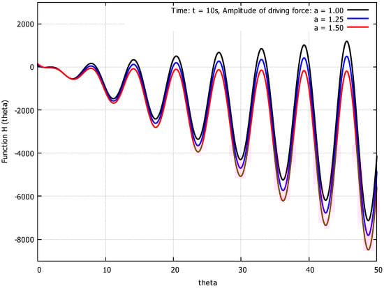
Figure 1. The function $H\left(\theta \right)$ for a nonlinear, damped and driven pendulum is plotted versus the amplitude of the forcing function, a, and the pendulum displacement, $\theta$, for the fixed value of $t=10$ s (after Das and Musielak [134]).

• Summary of the main results:

${\mathsf{\Phi }}_{\theta }(\theta ,t)$ is non-oscillatory and real — linear system with periodic motion;

${\mathsf{\Phi }}_{\theta }(\theta ,t)$ is oscillatory and complex—nonlinear system with periodic motion;

${\mathsf{\Phi }}_{\theta }(\theta ,t)$ is oscillatory and imaginary—nonlinear system with non-periodic motion.

The null Lagrangian is given by $L_n(\dot{\theta },\theta ,t)=d\mathsf{\Phi }/dt=[\dot{\theta }+q\theta +\alpha \left(t\right)]{\mathsf{\Phi }}_{\theta }$, which shows that only knowledge of ${\mathsf{\Phi }}_{\theta }(\theta ,t)$ is required. Thus, having obtained ${\mathsf{\Phi }}_{\theta }(\theta ,t)$ (see Equation (75)), $L_n(\dot{\theta },\theta ,t)$ can be evaluated and used to construct the following non-standard Lagrangian:

$$L_{ns}(\dot{\theta },\theta ,t)=[\dot{\theta }+q\theta +\alpha \left(t\right)]·{sinh}^{-1}\left(L_n\right)-{\displaystyle \frac{1}{{\mathsf{\Phi }}_{\theta }}}·\sqrt{1+{\left(L^n\right)}^2}.$$

(76)

Substitution of this NSL into the E-L equation gives the equation of motion (see Equation (72)).

The obtained results demonstrate that the gauge function plays the most fundamental role in describing classical dynamical systems because it uniquely determines the system’s transition from its periodic to non-periodic (chaotic) evolution, and it also allows finding both null and non-standard Lagrangians. These novel results presented in [134] were obtained without solving the equation of motion, or using the Lyapunov exponent or Poincaré sections.

8. Concluding Remarks and Perspectives

This paper presents a broad review of the basic concepts of the Lagrangian formalism that has been a powerful method to obtain equations of motion in modern physics. The concept of action and its Lagrangians are introduced, and Helmholtz’s conditions for the existence of Lagrangians are presented and discussed. Two families of Lagrangians, namely, standard and non-standard, are described, and different methods to derive them are reviewed. It is pointed out that there are no general methods to construct standard and non-standard Lagrangians from first principles. Nevertheless, there are many interesting examples of such Lagrangians obtained for different equations of motion, and some of them are presented and discussed in this review paper.

However, the main objective of this paper is to review the so-called null Lagrangians, often called trivial in mathematics, and their applications to different areas of modern physics. There are two basic properties of null Lagrangians: (i) they identically satisfy the E-L equation, and (ii) they are easy to construct because the total derivative of any scalar, smooth and differentiable function, also called a gauge function, is a null Lagrangian; these properties make them very different from standard and non-standard Lagrangians. Null Lagrangians have been extensively studied in mathematics, but their physical applications were very limited because they did not give any equation of motion.

In the last several years, the situation has changed as null Lagrangians and their gauge functions have been used to account for forces and nonlinearities in classical dynamical systems, and also to make some standard Lagrangians to be Galilean invariant, like the one for Newton’s first law of dynamics. In some studies, null Lagrangians have also been used in classical field theories, quantum mechanics, and in population dynamics, and all these applications of null Lagrangians are reviewed and discussed in this paper. However, a special emphasis is given to the most recent results, which demonstrate that gauge functions play the most fundamental roles in classical dynamics as they can be used to predict the future states of dynamical systems, without solving the equations of motion, as well as to construct their non-standard Lagrangians.

This recent work that shows fundamental roles play by the gauge functions in classical dynamical systems has been applied to a nonlinear, damped and driven pendulum with the main results summarized above. However, applications to other dynamical systems still remain to be conducted, especially to multi-dimensional nonlinear dynamical systems. Once the approach is generalized to multi-dimensional systems, then it can also be applied to classical and quantum fields located in 3D Galilean space and 4D flat or curved spacetime.

Studies of null Lagrangians and gauge functions as well as non-standard Lagrangians constructed from these gauge functions may reveal hidden symmetries in both equations of motion and and their Lagrangians. The fact that different equations of motion may have different symmetries, and that symmetries of such equations may be different than symmetries of their Lagrangians is well-established [21,22,23]. Moreover, it is also known that symmetries of equations of motions and their Lagrangians are directly related to Lie groups [11,29]. In general, if a Lagrangian is invariant with respect to rotations and translations, this may indicate the presence of the underlying Lie group (e.g., [139], and references therein). Future studies of symmetries and their underlying Lie groups in dynamical systems would lead to a better understanding of their evolution in time and space including transitions to non-periodic (chaotic) dynamical states, but also their interactions with the environment.

The roles played by null Lagrangians and gauge functions in physics described in this review paper are limited to classical one-dimensional dynamical systems and to selected quantum systems. The recent developments in this field presented in this review paper clearly demonstrate that a gauge function becomes a new and powerful tool to study dynamical systems. However, it is not any gauge function but a very special one, uniquely determined for a given system. Then, this unique gauge function is sufficient to peform system’ stability analysis, to predict its dynamical state, and to find its non-standard Lagrangian. The most important result is that this full physical description of the system is obtained without solving its equation of motion, and analyzing the resulting solutions. Thus, one of the most promising directions of future research would be the extension of these results to multi-dimensional systems, classical and quantum fields, and also to other areas of modern physics.

We hope that this paper presents a balanced view of null Lagrangians and the gauge functions, and their roles and applications in classical and quantum dynamics. It is also our hope that the selection of topics covered in this review paper reflects the previous and current research in this field well. The main purpose of this review paper will be accomplished if it serves as a guide to novel achievements in the field, and as an inspiration to scientists and students for opening new frontiers of research on null Lagrangians and gauge functions in different areas of theoretical physics.

Finally, let us point out that our reference list is only a small subset of all papers and books published by mathematicians and physicists on standard, non-standard and null Lagrangians. Our main preference was to cite all references directly relevant to the topics covered in this review paper. However, we do respect that other scientists working in the field may have different opinions in this matter.

References

- Euler, L. Methodus Inveniendi Lineas Curvas Maximi Minimive Proprietate Gaudentes; Springer Science & Business Media: Lausanne, Switzerland; Geneva, Switzerland, 1744. [Google Scholar]
- Lagrange, J.L. Analytical Mechanics; Springer: Dordrecht, The Netherlands, 1997. [Google Scholar]
- Hamilton, W.R. On a General Method in Dynamics; By Which the Study of the Motions of All Free Systems of Attracting or Repelling Points is Reduced to the Search and Differentiation of One Central Relation, or Characteristic Function. Phil. Trans. R. Soc. Lond. 1834, 124, 247. [Google Scholar]
- Landau, L.D.; Lifschitz, E.M. Mechanics; Pergamon Press: Oxford, UK, 1969. [Google Scholar]
- Goldstein, H.; Poole, C.P.; Safko, J.L. Classical Mechanics, 3rd ed.; Addison-Wesley: San Francisco, CA, USA, 2002. [Google Scholar]
- José, J.V.; Saletan, E.J. Classical Dynamics; A Contemporary Approach; Cambridge University Press: Cambridge, UK, 2002. [Google Scholar]
- Arnold, V.I. Mathematical Methods of Classical Mechanics; Springer: New York, NY, USA, 1978. [Google Scholar]
- Doughty, N.A. Lagrangian Interactions; Addison-Wesley: New York, NY, USA, 1990. [Google Scholar]
- Olver, P.J. Applications of Lie Groups to Differential Equations; Springer: New York, NY, USA, 1993. [Google Scholar]
- Grigore, D.R. Variational equations and symmetries in the Lagrangian formalism. J. Phys. A 1995, 28, 2921. [Google Scholar] [CrossRef]
- Vitolo, R. On different geometric formulations of Lagrangian formalism. Diff. Geom. Appl. 1999, 10, 225–255. [Google Scholar] [CrossRef]
- Crampin, M.; Saunders, D.J. The Hilbert-Carathéodory form for parametric multiple integral problems in the calculus of variations. Acta Appl. Math. 2003, 76, 37. [Google Scholar] [CrossRef]
- Crampin, M.; Saunders, D.J. On null Lagrangians. Diff. Geom. Appl. 2005, 22, 131. [Google Scholar] [CrossRef]
- Krupka, D.; Krupkova, O.; Saunders, D. The Cartan form and its generalizations in the calculus of variations. Int. J. Geom. Meth. Mod. Phys. 2010, 7, 631. [Google Scholar] [CrossRef]
- Anderson, D.R.; Carlson, D.E.; Fried, J. A continuum-mechanical theory for nematic elastomers. Elasticity 1999, 56, 35. [Google Scholar] [CrossRef]
- Saccomandi, G.; Vitolo, R.; Fried, J. Null Lagrangians for nematic elastomers. J. Math. Sci. 2006, 136, 4470. [Google Scholar] [CrossRef]
- Olver, P.J. Boundary conditions and null Lagrangians in the calculus of variations and elasticity. J. Elast. 2024, 155, 75. [Google Scholar] [CrossRef]
- Helmholtz, H.; Reine, J. Ueber die physikalische Bedeutung des Princips der kleinsten Wirkung. J. Reine Angew. Math. 1887, 100, 137. [Google Scholar] [CrossRef]
- Helmholtz, H. On the physical meaning of the principle of least action. J. Reine Angew Math. 1887, 100, 213. [Google Scholar] [CrossRef]
- Douglas, J. Solution of the inverse problem of the calculus of variations. Trans. Am. Math. Soc. 1941, 50, 71. [Google Scholar] [CrossRef]
- Hojman, S.A.; Urrutia, L.F. On the inverse problem of the calculus of variations. J. Math. Phys. 1981, 22, 1896. [Google Scholar] [CrossRef]
- Lopuszanski, J. The Inverse Variational Problems in Classical Mechanics; World Scientific: Singapore, 1999. [Google Scholar]
- Hojman, S.A. Symmetries of Lagrangians and of their equations of motion. J. Phys. A Math. Gen. 1984, 17, 2399–2412. [Google Scholar] [CrossRef]
- Musielak, Z.E.; Roy, D.; Swift, L.D. Method to derive Lagrangian and Hamiltonian for a nonlinear dynamical system with variable coefficients. Chaos Soliton Fract. 2008, 38, 894–902. [Google Scholar] [CrossRef]
- Musielak, Z.E. Standard and non-standard Lagrangians for dissipative dynamical systems with variable coefficients. J. Phys. A Math. Theor. 2008, 41, 055205. [Google Scholar] [CrossRef]
- Cieśliński, J.L.; Nikiciuk, T. A direct approach to the construction of standard and non-standard Lagrangians for dissipative-like dynamical systems with variable coefficients. J. Phys. A Math. Gen. 2010, 43, 175205. [Google Scholar] [CrossRef]
- Pham, D.T.; Musielak, Z.E. Novel roles of standard Lagrangians in population dynamics modeling and their ecological implications. Mathematics 2023, 11, 3653. [Google Scholar] [CrossRef]
- Nikiforov, A.F.; Uvarov, V.B. Special Functions of Mathematical Physics; Springer: Basel, Switzerland, 1988. [Google Scholar]
- Mathai, A.M.; Haubold, H.J. Special Functions for Applied Scientists; Springer: New York, NY, USA, 2008. [Google Scholar]
- Musielak, Z.E.; Davachi, N.; Rosario-Franco, M. Special functions of mathematical physics: A Unified Lagrangian Formalism. Mathematics 2020, 8, 379. [Google Scholar] [CrossRef]
- Musielak, Z.E.; Davachi, N.; Rosario-Franco, M.J. Lagrangians, gauge transformations and Lie groups for semigroup of second-order differential equations. J. Appl. Math. 2020, 2020, 3170130. [Google Scholar] [CrossRef]
- Bauer, P.S. Dissipative dynamical systems: I. Proc. Natl. Acad. Sci. USA 1931, 17, 311. [Google Scholar] [CrossRef] [PubMed]
- Bateman, H. On dissipative systems and related variational principles. Phys. Rev. 1931, 38, 815. [Google Scholar] [CrossRef]
- Caldirola, P. Forze non conservative nella meccanica quantistica. Nuovo Cim. 1941, 18, 393–400. [Google Scholar] [CrossRef]
- Kanai, E. On the quantization of the dissipative systems. Prog. Theor. Phys. 1948, 3, 44. [Google Scholar] [CrossRef]
- Vujanovic, B.D.; Jones, S.E. (Eds.) Variational Methods in Nonconservative Phenomena; Academic Press: New York, NY, USA, 1989; Volume 182, pp. 1–371. [Google Scholar]
- Vestal, L.C.; Musielak, Z.E. Bateman Oscillators: Caldirola-Kanai and Null Lagrangians and Gauge Functions. Physics 2021, 3, 449–458. [Google Scholar] [CrossRef]
- Torres del Castillo, G.F. Comment on “The one-dimensional harmonic oscillator damped with Caldirola-Kanai Hamiltonian”. Rev. Mex. Fisica 2019, 65, 103. [Google Scholar] [CrossRef]
- Ray, J.R. Lagrangians and systems they describe-how not to treat dissipation in Quantum Mechanics. Am. J. Phys. 1979, 47, 47. [Google Scholar] [CrossRef]
- Segovia-Chaves, F. The one-dimensional harmonic oscillator damped with Caldirola-Kanai Hamiltonian. Rev. Mex. Fisica 2019, 64, 626. [Google Scholar] [CrossRef]
- Riewe, F. Nonconservative Lagrangian and Hamiltonian mechanics. Phys. Rev. E 1996, 53, 1890. [Google Scholar] [CrossRef]
- Riewe, F. Mechanics with fractional derivatives. Phys. Rev. E 1997, 55, 3581. [Google Scholar] [CrossRef]
- Bersani, A.M.; Caressa, P. Lagrangian descriptions of dissipative systems: A review. Math. Mech. Solids 2020, 26, 785. [Google Scholar] [CrossRef]
- Pham, D.T.; Musielak, Z.E. Non-standard and null Lagrangians for nonlinear dynamical systems and their role in in population dynamics. Mathematics 2023, 11, 2671. [Google Scholar] [CrossRef]
- Jimenez, J.L.; Del Valle, G.; Campos, I. A canonical treatment of some systems with friction. Eur. J. Phys. 2005, 26, 711–725. [Google Scholar] [CrossRef]
- Chandrasekar, V.K.; Senthilvelan, M.; Lakshmanan, M. On the complete integrability and linearization of nonlinear ordinary differential euqations. Part II: Thrid order equations. Proc. Royal Soc. A Math. Phys. Eng. Sci. 2006, 462, 1831. [Google Scholar]
- Carineña, J.F.; Ranada, M.F.; Santander, M. Lagrangian formalism for nonlinear second-order Riccati systems: One-dimensional integrability and two-dimensional superintegrability. J. Math. Phys. 2005, 46, 062703. [Google Scholar] [CrossRef]
- Musielak, Z.E. General conditions for the existence of non-standard Lagrangians for dissipative dynamical systems. Chaos Solitons Fractals 2009, 42, 2645–2652. [Google Scholar] [CrossRef]
- Davachi, N.; Musielak, Z.E. Generalized non-standard Lagrangians. J. Undergrad. Rep. Phys. 2019, 29, 100004. [Google Scholar] [CrossRef]
- Saha, A.; Talukdar, B. Inverse variational problem for non-standard Lagrangians. Rep. Math. Phys. 2014, 73, 299–309. [Google Scholar] [CrossRef]
- Pham, D.T.; Musielak, Z.E. Review of Lagrangian formalism in biology: Recent advances and perspectives. Acad. Biol. 2024, 2. [Google Scholar] [CrossRef]
- Jacobi, C.G.J. Sur un noveau principe de la méanique analytique. C.R. Acad. Sci. Paris 1842, 15, 202. [Google Scholar]
- Nucci, M.C.; Leach, P.G.L. Lagrangians galore. J. Math. Phys. 2007, 48, 123510. [Google Scholar] [CrossRef]
- Nucci, M.C.; Leach, P.G.L. Jacobi last multiplier and Lagrangians for multidimensional linear systems. J. Math. Phys. 2008, 49, 073517. [Google Scholar] [CrossRef]
- Nucci, M.C.; Leach, P.G.L. The Jacobi’s Last Multiplier and its applications in mechanics. Phys. Scr. 2008, 78, 065011. [Google Scholar] [CrossRef]
- Nucci, M.C.; Tamizhmani, K.M. Lagrangians for dissipative nonlinear oscillators: The method of last Jacobi multiplier. J. Nonlinear Math. Phys. 2010, 17, 167. [Google Scholar] [CrossRef]
- Nucci, M.C.; Leach, P.G.L. Some Lagrangians for systems without a Lagrangian. Phys. Scr. 2011, 83, 035007. [Google Scholar] [CrossRef]
- Nucci, M.C.; Tamizhmani, K.M. Lagrangians for biological models. J. Nonlinear Math. Phys. 2012, 19, 1250021. [Google Scholar] [CrossRef]
- Nucci, M.C.; Sanchini, G. Symmetries, Lagrangians and Conservation Laws of an Easter Island Population Model. Symmetry 2015, 7, 1613–1632. [Google Scholar] [CrossRef]
- Trubatch, S.L.; Franco, A. Canonical procedures for population dynamics. J. Theor. Biol. 1974, 48, 299–324. [Google Scholar] [CrossRef]
- Paine, G.H. The development of Lagrangians for biological models. Bull. Math. Biol. 1982, 44, 749–760. [Google Scholar] [CrossRef]
- Choudhury, A.G.; Guha, P.; Khanra, B. On the Jacobi last multiplier, integrating factors and the Lagrangian formulation of differential equations of the Painlevé–Gambier classification. J. Math. Anal. Appl. 2009, 360, 65. [Google Scholar] [CrossRef]
- Cariñena, J.F.; Fernandez-Nuñez, J. Some Applications of Affine in Velocities Lagrangians in Two-Dimensional Systems. Symmetry 2022, 14, 2520. [Google Scholar] [CrossRef]
- Cariñena, J.F.; Fernandez-Nuñez, J. Jacobi Multipliers in Integrability and the Inverse Problemof Mechanics. Symmetry 2022, 14, 2520. [Google Scholar]
- Cariñena, J.F.; de Lucas, J.; Rañada, M.F. Jacobi multipliers, non-local symmetries, and nonlinear oscillators. J. Math. Phys. 2015, 56, 063505. [Google Scholar] [CrossRef]
- Cariñena, J.F.; Rañada, M.F. Jacobi multipliers and Hojman symmetry. Int. J. Geom. Meth. Mod. Phys. 2021, 18, 2150166. [Google Scholar] [CrossRef]
- Cariñena, J.F.; Santos, P. Jacobi multipliers and Hamel’s formalism. J. Phys. A Math. Theor. 2021, 54, 225203. [Google Scholar] [CrossRef]
- El-Nabulsi, R.A. A fractional appraoch of nonconservative Lagrangian dynamics. Fizika A 2005, 14, 289. [Google Scholar]
- El-Nabulsi, R.A. A periodic functional approach to the calculus of variations and the problem of time-dependent damped harmonic oscillators. App. Math. Lett. 2011, 24, 1647. [Google Scholar]
- El-Nabulsi, R.A. Nonlinear dynamics with non-standard Lagrangians. Qual. Theory Dyn. Syst. 2013, 12, 273–291. [Google Scholar] [CrossRef]
- El-Nabulsi, R.A. Fractional oscillators from non-standard Lagrangians with time-dependent fractional oscillators. Comm. App. Math. 2014, 33, 163. [Google Scholar]
- El-Nabulsi, R.A. Non-standard power-law Lagrangians in classical and quantum dynamics. App. Math. Lett. 2015, 43, 120. [Google Scholar] [CrossRef]
- El-Nabulsi, R.A. Fractional derivatives generalization of Einstein’s field equations. Indian J. Phys. 2013, 87, 195–200. [Google Scholar] [CrossRef]
- El-Nabulsi, R.A. Fractional action cosmology with variable order parameter. Int. J. Theor. Phys. 2017, 56, 1159–1182. [Google Scholar] [CrossRef]
- El-Nabulsi, R.A. Non-standard magnetohydrodynamics equations and their implications in sunspots. Proc. R. Soc. A 2020, 476, 20200190. [Google Scholar] [CrossRef]
- El-Nabulsi, R.A. On a new fractional uncertainty relation and its implications in quantum mechanics and molecular physics. Proc. Math. Phys. Eng. Sci. 2020, 476, 1. [Google Scholar] [CrossRef]
- El-Nabulsi, R.A. Logarithmic Lagrangian matter density, unimodular gravity-like and accelerated expansion with a negative cosomological constant. J. Korean Phys. Soc. 2021, 79, 345E. [Google Scholar] [CrossRef]
- El-Nabulsi, R.A.; Anukool, W. A new approach to nonlinear quartic oscillators. Arch. App. Mech. 2022, 92, 351. [Google Scholar] [CrossRef]
- Mathews, P.M.; Lakshmanan, M. On a unique nonlinear oscillator. Q. Appl. Math. 1974, 32, 215. [Google Scholar] [CrossRef]
- Lakshmanan, M.; Rajasekar, S. Nonlinear Dynamics: Integrability, Chaos and Patterns; Springer: Berlin/Heidelberg, Germany, 2003. [Google Scholar]
- Khana, B.A.; Chatterjeeb, S.; Alic, S.G.; Talukdard, B. Inverse Variational Problem for Nonlinear Dynamical Systems. Acta Phys. Polonica A 2022, 141, 64. [Google Scholar] [CrossRef]
- Havas, P. The range of application of the Lagrange formalism—I. Nuovo Cimento 1957, 5, 363. [Google Scholar] [CrossRef]
- Gonzalez, G. Comment on “Standard and non-standard Lagrangians for dissipative dynamical systems with variable coefficients”. arXiv 2022, arXiv:2202.05391v1. [Google Scholar]
- Chandrasekar, V.K.; Senthilvelan, M.; Lakshmanan, M. Unusual Liénard-type nonlinear oscillator. Phys. Rev. E 2005, 72, 066203. [Google Scholar] [CrossRef]
- Kudryashov, N.A.; Sinelshchikov, D. New non-standard Lagrangians for the Liénard-type oscillator. Appl. Math. Lett. 2017, 63, 124. [Google Scholar] [CrossRef]
- Carinena, J.F.; Ranada, M.F.; Santander, M.; Senthilvelan, M. A non-linear oscillator with quasi-harmonic behaviour: Two- and n-dimensional oscillators. Nonlinearity 2004, 17, 1941–1963. [Google Scholar] [CrossRef]
- Udwadia, F.E.; Cho, H. Lagrangians for damped linear multi-degree-of-freedom systems. J. Appl. Mech. 2013, 80, 041023. [Google Scholar] [CrossRef]
- Alekseev, A.I.; Arbuzov, B.A. Classical Yang-Mills field theory with non-standard Lagrangians. Theor. Math. Phys. 1984, 59, 372. [Google Scholar] [CrossRef]
- Supanyo, S.; Tanasittikosol, M.; Yoo-Kong, S. Natural TeV cutoff of the Higgs field from a multiplicative Lagrangian. Phys. Rev. D 2022, 106, 035020. [Google Scholar] [CrossRef]
- Supanyo, S.; Tanasittikosol, M.; Yoo-Kong, S. Nonstandard Lagrangians for a real scalar field and a fermion field from the nonuniqueness principle. Theor. Math. Phys. 2024, 221, 1695. [Google Scholar] [CrossRef]
- Vestal, L.C.; Musielak, Z.E. Gauge functions for forces and nonlinearities in classical oscillators. J. Appl. Nonlinear Dyn. 2024, 13, 837. [Google Scholar] [CrossRef]
- Musielak, Z.E. Nonstandard Null Lagrangians and Gauge Functions for Newtonian Law of Inertia. Physics 2021, 3, 903–912. [Google Scholar] [CrossRef]
- Edelen, D.G. The nul set of the Euler-Lagrange operator. Arch. Rotat. Mech. Anal. 1962, 11, 117. [Google Scholar] [CrossRef]
- Krupka, D. Some geometric aspects of variational problems in fibred manifolds. Folia Fac. Sci. Nat. Univ. Purk. Brun. Phys. 1973, 14, 65. [Google Scholar]
- Krupka, D. A map associated to the Lepagian forms on the calculus of variations in fibred manifolds. Czechoslovak Math. J. 1977, 27, 114. [Google Scholar] [CrossRef]
- Crampin, M. Constants of the motion in Lagrangian mechanics. Int. J. Theor. Phys. 1977, 16, 741. [Google Scholar] [CrossRef]
- Hojman, S.A. A new conservation law constructed without using Lagrangians or Hamiltonians. J. Phys. A Math. Gen. 1992, 25, L291. [Google Scholar] [CrossRef]
- Betounes, D.E. Differential geometric aspects of the Cartan form: Symmetry theory. J. Math. Phys. 1987, 28, 2347. [Google Scholar] [CrossRef]
- Olver, P.J.; Sivaloganathan, J. The structure of null Lagrangians. Nonlinearity 1988, 1, 389. [Google Scholar] [CrossRef]
- Giaquinta, M.; Hilderbrandt, S. Calculus of Variations I; Springer: Berlin/Heidelberg, Germany, 1996. [Google Scholar]
- Hojman, S. Problem of the identical vanishing of Euler-Lagrange derivatives in field theory. Phys. Rev. D 1983, 27, 451. [Google Scholar] [CrossRef]
- Krupka, D.; Musilova, J. Trivial Lagrangians in field theory. Diff. Geom. Appl. 1998, 9, 293. [Google Scholar] [CrossRef]
- Grigore, D.R. Trivial Second-Order Lagrangians in classical field theory. Progr. Phys. 1999, 47, 913. [Google Scholar] [CrossRef]
- Ericksen, J.L. Nilpotent energies in liquid crystal theory. Arch. Rotat. Mech. Anal. 1962, 10, 189. [Google Scholar] [CrossRef]
- Levy-Leblond, J.-M. Group-theoretical foundations of classical mechanics: The Lagrangian gauge problem. Commun. Math. Phys. 1969, 12, 64–79. [Google Scholar] [CrossRef]
- Musielak, Z.E.; Watson, T.B. Gauge functions and Galilean invariance of Lagrangians. Phys. Lett. A 2020, 384, 126642. [Google Scholar] [CrossRef]
- Musielak, Z.E.; Watson, T.B. General null Lagrangians, exact gauge functions and forces in Newtonian mechanics. Phys. Lett. A 2020, 384, 126838. [Google Scholar] [CrossRef]
- Musielak, Z.E.; Vestal, L.C.; Tran, B.D.; Watson, T.B. Gauge functions in classical mechanics: From undriven to driven dynamical systems. Physics 2020, 2, 425–435. [Google Scholar] [CrossRef]
- Segovia, A.L.; Vestal, L.C.; Musielak, Z.E. Nonstandard null Lagrangians and gauge functions and dissipative forces in dynamics. Phys. Lett. A 2022, 453, 128457. [Google Scholar] [CrossRef]
- Dange, A.A.; Vestal, L.C.; Musielak, Z.E. Generalized null Lagrangians for equations with special function solutions. J. Undergrad. Rep. Phys. 2021, 30, 2. [Google Scholar] [CrossRef]
- Filyukov, S.; Masterov, I. Generalized Schwarzian mechanics. Nucl. Phys. B 2021, 964, 115316. [Google Scholar] [CrossRef]
- Kryński, W. The Schwarzian derivative and Euler–Lagrange equations. J. Geom. Phys. 2022, 182, 104665. [Google Scholar] [CrossRef]
- Majhi, P.; Panja, M.M.; Sarkar, P.; Talukdar, B. Null Lagrangians in Schwarzian mechanics. Phys. Lett. A 2025, 530, 130092. [Google Scholar] [CrossRef]
- Galajinsky, A. Schwarzian mechanics via nonlinear realizations. Phys. Lett. B 2019, 795, 277. [Google Scholar] [CrossRef]
- Goddard, P.; Olive, D. Kac-Moody and Virasoro algebras in relation to quantum physics. Int. J. Mod. Phys. A 1986, 1, 303. [Google Scholar] [CrossRef]
- Aharonov, D. A necessary and sufficient condition for univalence of a meromorphic function. Duke Math. J. 1969, 36, 599. [Google Scholar] [CrossRef]
- Tamanoi, H. Higher-order Schwarzian operators and combinatorics of the Schwarzian derivative. Math. Ann. 1996, 305, 127. [Google Scholar] [CrossRef]
- Kim, S.; Sugawa, T. Invariant Schwarzian derivatives of higher order. Complex Anal. Oper. Theory 2011, 5, 659. [Google Scholar] [CrossRef]
- Krivonos, S. Origin of higher Schwarzians. Phys. Rev. D 2024, 109, 065029. [Google Scholar] [CrossRef]
- Vankerschaver, J.; Liao, C.; Leok, M. Generating functionals and Lagrangian partial differential equations. J. Math. Phys. 2013, 54, 082901. [Google Scholar] [CrossRef]
- Christodoulou, D. The Action Principle and Partial Differential Equations; Princeton University Press: Princeton, NJ, USA, 2016. [Google Scholar]
- Ball, M.; Currie, J.C.; Olver, P.J. Null Lagrangians, weak continuity, and variational problems of arbitrary order. J. Funct. Anal. 1981, 41, 135. [Google Scholar] [CrossRef]
- Crampin, M. Gaussian curvature as a null homogeneous second-order Lagrangian. Publ. Math. Debrecen 2003, 62, 351. [Google Scholar] [CrossRef]
- Scholle, M. Construction of Lagrangians in continuum theories. Proc. R. Soc. Lond. 2004, 460, 3241. [Google Scholar] [CrossRef]
- Kovalev, V.A.; Radaev, Y.N. Forms of null Lagrangians in field theories of continuum mechanics. Mech. Solids 2012, 47, 137. [Google Scholar] [CrossRef]
- Whitman, G.B. Linear and Nonlinear Waves; John Wiley & Sons, Inc.: New York, NY, USA, 1999. [Google Scholar]
- Musielak, Z.E. Standard Lagrangians for wave, Laplace and Tricomi-like equations with variable coefficients. J. Phys. A Math. Theor. 2010, 43, 425205. [Google Scholar] [CrossRef]
- Musielak, Z.E. A new fundamental asymmetric wave equation and its application to acoustic wave propagation. Adv. Math. Phys. 2023, 2023, 57366419. [Google Scholar] [CrossRef]
- El-Nabulsi, A.R. Nonlinear wave equation in an inhomogeneous medium from non-standard singular Lagrangians functional with two occurrences of integrals. Int. J. Nonlinear Sci. Num. Simul. 2020, 20, 761. [Google Scholar] [CrossRef]
- Thieme, K. Null Lagrangians of non-local field theories. arXiv 2020, arXiv:2009.13499. [Google Scholar] [CrossRef]
- Vestal, L.C. Novel Roles of Standard and Non-Standard Null Lagrangians in Classical and Quantum Physics. Ph.D. Thesis, The University of Texas at Arlington, Arlington, TX, USA, 2023. [Google Scholar]
- Das, R.; Musielak, Z.E. General null Lagrangians and their novel role in classical dynamics. Phys. Scr. 2022, 97, 125213. [Google Scholar] [CrossRef]
- Das, R.; Musielak, Z.E. New role of null lagrangians in derivation of equations of motion for dynamical systems. Phys. Scr. 2023, 98, 045201. [Google Scholar] [CrossRef]
- Das, R.; Musielak, Z.E. Fundamental roles of gauge functions in classical dynamics. EPL 2025, 150, 33002. [Google Scholar] [CrossRef]
- Baker, G.L.; Gollub, J.P. Chaotic Dynamics: An Introduction, 2nd ed.; Cambridge University Press: New York, NY, USA, 1996. [Google Scholar]
- Taylor, J.R. Classical Mechanics; University Science Books: Sausalito, CA, USA, 2005. [Google Scholar]
- Moon, F.C. Chaotic and Fractal Dynamics; John Wiley & Sons: New York, NY, USA, 1992. [Google Scholar]
- Bevivino, J. Dynamics at Horsetooth; Colorado State University: Fort Collins, CO, USA, 2009; Volume 1. [Google Scholar]
- Muzsnay, Z.; Thompson, G. Inverse problem of the calculus of variations on Lie groups. Diff. Geom. Appl. 2005, 23, 257. [Google Scholar] [CrossRef]
Disclaimer/Publisher’s Note: The statements, opinions and data contained in all publications are solely those of the individual author(s) and contributor(s) and not of MDPI and/or the editor(s). MDPI and/or the editor(s) disclaim responsibility for any injury to people or property resulting from any ideas, methods, instructions or products referred to in the content. |
© 2025 by the authors. Licensee MDPI, Basel, Switzerland. This article is an open access article distributed under the terms and conditions of the Creative Commons Attribution (CC BY) license (https://creativecommons.org/licenses/by/4.0/).