Prescribed-Performance-Function-Based RISE Control for Electrohydraulic Servo Systems with Disturbance Compensation

Abstract

Considering that the electrohydraulic servo system has extremely strong nonlinear characteristics, problems such as low initial tracking accuracy and large unmodeled dynamic errors are prominent, leading to easy degradation of control performance. To achieve high-precision position tracking control, this study proposes a robust integral of the sign of the error (RISE) control method with prescribed performance function (PPF) and dual extended state observers (DESOs). Combined with the system dynamic model, DESOs are designed to estimate matched and mismatched uncertainties, respectively. The transformed error signal is obtained based on the prescribed performance function (PPF), while restricting the convergence rate and range of the error. A RISE controller is designed using the backstepping method to suppress both matched and unmatched uncertainties and improve the system robustness. The Lyapunov stability theory proves that the system is semi-globally stable and all signals are bounded. Simulation results show that the proposed control strategy significantly improves the tracking accuracy and error convergence rate of the electrohydraulic servo system, fully verifying the effectiveness of the control strategy.

1. Introduction

Electrohydraulic servo systems are widely used in coal mining, heavy-duty engineering operations, and other fields due to their high power-to-weight ratio, reliability, and maintainability [1,2]. However, due to the strong nonlinearity and unmodeled uncertainties of such systems, achieving high-precision position control for electrohydraulic servo systems is more difficult than that for motor-driven systems [3]. The main factor is that electrohydraulic servo systems rely on multiple external sensing elements to obtain system state feedback, such as position, pressure, and flow sensors. During the initial stage of system movement, the error accumulation among various sensors leads to large errors, which affects the position tracking accuracy of the system to a certain extent [4].

High-precision control of hydraulic systems is crucial to ensure the system operates according to the expected trajectory. In the field of nonlinear control theory, methods such as sliding mode control, adaptive control, and robust control are widely used in hydraulic systems. To address the contradiction between convergence speed and chattering in traditional sliding mode surface design, prescribed performance function (PPF) provides a new idea by constructing a performance function to constrain the transient and steady-state behaviors of tracking errors [5,6,7]. In recent years, researchers have combined PPF with various control methods. For example, Guo et al. [8] proposed an adaptive backstepping control based on PPF, which effectively suppresses the parameter uncertainties of electrohydraulic servo systems; Zeng et al. [9] combined PPF with the adaptive learning method to achieve accurate position control of electrohydraulic servo systems. However, existing studies do not fully consider the external disturbances encountered by electrohydraulic servo systems during operation, including matched and mismatched uncertainties.

In recent years, significant progress has been made in the field of fluid power transmission and control regarding hydraulic system modeling and compensation. Wang et al. [10] proposed an improved nonlinear model considering oil compressibility and pipeline dynamics, laying a foundation for high-precision control. Literature [11,12,13] proposed compensation strategies for the nonlinear flow characteristics and pressure dynamics of valve-controlled asymmetric cylinders, respectively. In particular, Feng et al. [14] verified the improvement effect of friction compensation on the low-speed performance of hydraulic systems through experiments. In terms of parameter identification, intelligent algorithms such as particle swarm optimization [15,16] and deep reinforcement learning [17,18] have been introduced to improve model accuracy. However, most existing compensation methods rely on accurate models, and their adaptability to system parameter perturbations and uncertain disturbances needs to be improved.

The research on position control of electrohydraulic servo systems shows a trend from actuator on-off control to high-precision valve control. Traditional PID control is still widely used in industry due to its simple structure, but its performance is limited when dealing with nonlinear coupling [19,20,21]. To this end, scholars have proposed various solutions: Yao et al. [22,23] designed an adaptive robust controller to handle model uncertainties; Chen et al. [24] combined disturbance observers with the backstepping method to suppress external disturbances. It is worth noting that for trajectory tracking problems, Zhu et al. [25] verified the advantage of PPF in constraining tracking errors, but did not consider the dynamic characteristics of hydraulic actuators. In addition, most existing studies assume that the velocity signal is measurable, while in actual systems, velocity is often obtained through position differentiation, which also introduces the problem of noise amplification [26,27].

Combined with the current existing research methods, whether it is PPF, ESO or nonlinear control, each has relatively good performance. However, for actual physical systems, we often need to consider more and more complex scenarios. Therefore, we intend to improve and integrate the above-mentioned methods to realize the integrated design of the controller and enable it to possess the respective advantages of these methods. To solve the high-precision position tracking control problem of electrohydraulic servo systems under the interference of matched and mismatched uncertainties, this study proposes to combine the RISE control with the PPF and DESOs. Different from the previous concept of achieving high-precision tracking control for electro-hydraulic servo systems by designing complex nonlinear controllers, the method proposed in this study integrates the advantages of PPF and DESOs—which do not rely on complex calculation processes in their design. While ensuring fast, accurate, and highly robust control, it reduces the design difficulty of the controller itself and improves the convenience and rationality of parameter adjustment.

The remaining sections of this study are arranged as follows: Section 2 introduces the mathematical model of the single-degree-of-freedom electrohydraulic servo system; Section 3 describes the design of the PPF in detail; Section 4 presents the controller design and stability analysis process, including the design theory of DESOs and RISE controller; Section 5 verifies the effectiveness of the proposed control strategy through simulation examples; Section 6 discusses the research results and future plans.

2. Nonlinear Mathematical Model of Electrohydraulic Servo Systems

2.1. Dynamic Model of Single-Rod Hydraulic Cylinder

Combined with Newton’s dynamic theorem, the dynamic equation paradigm of the single-rod electrohydraulic servo system can be obtained as follows:

$$m\ddot{y}=\left(P_1{A}_1-P_2{A}_2\right)-B\dot{y}+{\mathrm{\Delta }}_1\left(t\right)$$

(1)

where $m$ denotes the end load mass of the electrohydraulic servo system; $x$, $\dot{x}$, and $\ddot{x}$ represent the displacement, velocity, and acceleration of the end load, respectively; $P_1$ and $P_2$ represent the pressures in the rodless chamber and rod chamber of the single-rod hydraulic cylinder, respectively; $A_1$ and $A_2$ represent the effective piston areas of the rodless chamber and rod chamber of the single-rod hydraulic cylinder, respectively; $B$ denotes the viscous friction coefficient existing during the system movement; ${\mathrm{\Delta }}_1\left(t\right)$ represents the unmatched uncertainty of the system, i.e., unknown disturbance, including unmodeled friction.

As shown in Figure 1, the servo valve is responsible for driving the hydraulic cylinder. The red lines represent the flow rate of Chamber 1, and the blue lines represent the flow rate of Chamber 2. The hydraulic cylinder is a single-rod cylinder, where 1 represents the rodless chamber and 2 represents the rod chamber. $P_{\mathrm{s}}$ and $P_{\mathrm{r}}$ represent the system supply pressure and return pressure, respectively; $F$ represents the output force of the electrohydraulic servo system; $P_L=P_1-P_2$ represents the pressure difference between the two chambers. The servo valve controls the flow rates at the inlet and outlet ports to achieve position control.

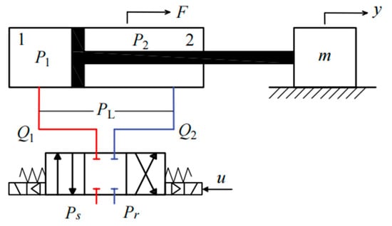
Figure 1. Schematic diagram of the single-rod electrohydraulic servo system.

Assumption 1.

The openings at both ends of the servo valve are regarded as a symmetric structure, and the dynamics of the servo valve are simplified to a proportional link.

Assumption 2.

Considering the compact layout of the device and the oil source, the oil sources of different chambers are regarded as having the same elastic modulus.

Without loss of generality, the pressure dynamic equation of the electrohydraulic servo system can be described as:

$$\left\{\begin{array}{l}{\dot{P}}_1={\displaystyle \frac{{\beta }_{\mathrm{e}}}{V_1}}\left(Q_1-A_1\dot{y}-C_{\mathrm{t}}{\dot{P}}_{\mathrm{L}}\right)+d_1\left(t\right)\\ {\dot{P}}_2={\displaystyle \frac{{\beta }_{\mathrm{e}}}{V_2}}\left(-Q_2+A_2\dot{y}+C_{\mathrm{t}}{\dot{P}}_{\mathrm{L}}\right)+d_2\left(t\right)\end{array}\right.$$

(2)

$$\left\{\begin{array}{l}{V}_1=V_{01}+A_{1}y\\ V_2=V_{02}-A_{2}y\end{array}\right.$$

(3)

where ${\beta }_{\mathrm{e}}$ denotes the elastic modulus of the hydraulic oil, which is a positive constant;$V_{10}$ and $V_{20}$ represent the initial volumes of the two chambers; $V_1$ and $V_2$ represent the actual volumes of the two chambers during movement; $Q_1$ and $Q_2$ represent the flow rates of the two chambers; $C_{\mathrm{t}}$ denotes the internal leakage coefficient; $d_1\left(t\right)$ and $d_2\left(t\right)$ represent the unmodeled uncertainties and external leakage existing in the establishment process of the two-chamber pressure dynamic model.

The servo valve adjusts the size of the valve port opening by adjusting the spool position, thereby changing the flow rates of oil flowing into and out of the actuator chambers. The flow equation of the servo valve can be expressed as:

$$\left\{\begin{array}{c}{Q}_1=k_{\mathrm{q}}{x}_{\mathrm{v}}\left(s\left(x_{\mathrm{v}}\right)\sqrt{P_{\mathrm{s}}-P_1}+s\left(x_{\mathrm{v}}\right)\sqrt{P_1-P_{\mathrm{r}}}\right)\\ Q_2=k_{\mathrm{q}}{x}_{\mathrm{v}}\left(s\left(x_{\mathrm{v}}\right)\sqrt{P_2-P_{\mathrm{r}}}+s\left(x_{\mathrm{v}}\right)\sqrt{P_{\mathrm{s}}-P_2}\right)\end{array}\right.$$

(4)

$$\left\{\begin{array}{l}{k}_{\mathrm{q}}=C_{\mathrm{d}}w\sqrt{{\displaystyle \frac{2}{\sigma }}}\\ x_{\mathrm{v}}=k_{\mathrm{u}}u\end{array}\right.$$

(5)

where $k_{\mathrm{q}}$ represents the flow gain at both ends of the servo valve spool displacement; $x_{\mathrm{v}}$ is the spool displacement of the servo valve; $k_{\mathrm{u}}$ represents the voltage gain of the servo valve.; $C_{\mathrm{d}}$ represents the flow coefficient of the servo valve orifice; $w$ is the area gradient of the orifice; $\sigma$ is the density of the hydraulic oil used in the system. The function $s\left(\ast \right)$ is defined as follows:

$$s\left(\ast \right)=\left\{\begin{array}{l}1, \mathrm{if} \ast \ge 0\\ 0, \mathrm{if} \ast <0\end{array}\right.$$

(6)

Therefore, Equation (4) of the electrohydraulic servo system can be rewritten as:

$$\left\{\begin{array}{l}{Q}_1=k_{\mathrm{t}}{R}_{1}u\\ Q_2=k_{\mathrm{t}}{R}_{2}u\end{array}\right.$$

(7)

where $k_{\mathrm{t}}=k_{\mathrm{q}}{k}_{\mathrm{u}}$. Meanwhile, there is:

$$\left\{\begin{array}{c}{R}_1=s\left(u\right)\sqrt{P_{\mathrm{s}}-P_1}+s\left(u\right)\sqrt{P_1-P_{\mathrm{r}}}\\ R_2=s\left(u\right)\sqrt{P_2-P_{\mathrm{r}}}+s\left(u\right)\sqrt{P_{\mathrm{s}}-P_2}\end{array}\right.$$

(8)

The actual output force of the electrohydraulic servo system can be expressed as:

$$F=A_1{P}_1-A_2{P}_2$$

(9)

2.2. State Space Function of Single-Rod Electrohydraulic Servo System

To facilitate the subsequent controller design and analysis, define the state variables $x={[x_1,x_2,x_3]}^{\mathrm{T}}$ where $x_1=y$, $x_2={\dot{x}}_1$, $x_3=A_1{P}_1-A_2{P}_2=F$. Combined with the above equations, the nonlinear dynamic model of the single-rod electrohydraulic servo system can be expressed in the form of the following state space function:

$$\left\{\begin{array}{l}{\dot{x}}_1=x_2\\ {\dot{x}}_2={\displaystyle \frac{1}{m}}\left[x_3-B{x}_2+{\mathrm{\Delta }}_1\left(t\right)\right]\\ {\dot{x}}_3=f_{1}u-f_2-f_3+{\mathrm{\Delta }}_2\left(t\right)\end{array}\right.$$

(10)

$$\left\{\begin{array}{l}{f}_1\triangleq {\beta }_{\mathrm{e}}{k}_{\mathrm{t}}\left({\displaystyle \frac{A_1}{V_1}}{R}_1+{\displaystyle \frac{A_2}{V_2}}{R}_2\right)\\ f_2\triangleq {\beta }_{\mathrm{e}}\left({\displaystyle \frac{A_1^2}{V_1}}+{\displaystyle \frac{A_2^2}{V_2}}\right)x_2\\ f_3\triangleq {\beta }_{\mathrm{e}}{C}_{\mathrm{t}}\left({\displaystyle \frac{A_1}{V_1}}+{\displaystyle \frac{A_2}{V_2}}\right)P_{\mathrm{L}}\end{array}\right.$$

(11)

$${\mathrm{\Delta }}_2\left(t\right)=A_1{d}_1\left(t\right)-A_2{d}_2\left(t\right)$$

(12)

where the control input of the actuator in the single-rod electrohydraulic servo system is $u$.

Assumption 3.

The command trajectory tracked by the single-rod electrohydraulic servo system is three times differentiable, and the derivatives of all orders are bounded.

Assumption 4.

Each element in the mismatched uncertainty ${\mathrm{\Delta }}_1\left(t\right)$ and matched uncertainty ${\mathrm{\Delta }}_2\left(t\right)$ is sufficiently smooth, and the first and second derivatives of the elements exist and are bounded. The specific boundary definitions are provided in Theorem 1.

Regarding Assumptions 3 and 4, although the trajectories tracked by actual physical systems or the disturbances they are subjected to are often non-differentiable, the differentiability of their signals can be ensured by adopting filtering or continuous approximation methods.

3. Design of Prescribed Performance Function

The purpose of the prescribed performance function is to stabilize the control tracking error within a preset range, ensuring the stability of system tracking and the rapidity of error convergence. Before designing the prescribed performance function, the system tracking error is defined as follows:

$$e_1\triangleq x_1-x_{1\mathrm{d}}$$

(13)

To constrain the tracking error and ensure the specified transient and steady-state tracking performance, a positive exponentially decreasing function is established as follows:

$$\mu \left(t\right)=\left({\mu }_0-{\mu }_{\infty }\right)e^{-kt}+{\mu }_{\infty }$$

(14)

where ${\mu }_0$, ${\mu }_{\infty }$, and $k$ all constants greater than 0; $e$ represents the natural constant, an infinite non-repeating decimal.

When the following formula holds, the control objective can be achieved, i.e., the error is stabilized in an interval symmetric about the coordinate axis:

$$-\underset{\_}{\vartheta }\mu \left(t\right)<e_1\left(t\right)<\overline{\vartheta }\mu \left(t\right),\forall t>0$$

(15)

where $\underset{\_}{\vartheta }$ and $\overline{\vartheta }$ are both constants greater than 0. It can be clearly seen from the function that $-\underset{\_}{\vartheta }{\mu }_0$ and $\overline{\vartheta }{\mu }_0$ define the lower and upper bounds of the joint tracking error in the initial stage of tracking, respectively; the parameter $k$ limits the convergence rate of $\mu \left(t\right)$ and also limits the convergence rate of the error $e_1\left(t\right)$, $k$ is a constant greater than 0; $-\underset{\_}{\vartheta }{\mu }_{\infty }$ and $\overline{\vartheta }{\mu }_{\infty }$ represent the allowable steady-state range of the tracking error $e_1\left(t\right)$ when $t\to \infty$.

To guide the controller design, the constrained form of Equation (15) is transformed into an equivalent unconstrained form. For this purpose, a smooth and strictly increasing function $\psi \left(z_1\right)$ about $z_1\left(t\right)$ is introduced, which satisfies the following characteristics:

$$-\underset{\_}{\vartheta }<\psi \left(z_1\right)<\overline{\vartheta }, \forall z_1\in L_{\infty }$$

(16)

$$\left\{\begin{array}{l}{\lim }_{z_1\to +\infty }\psi \left(z_1\right)=\overline{\vartheta }\\ {\lim }_{z_1\to -\infty }\psi \left(z_1\right)=-\underset{\_}{\vartheta }\end{array}\right.$$

(17)

According to Equation (16), Equation (15) can be rewritten as:

$$e_1\left(t\right)=\mu \left(t\right)\psi \left(z_1\right)$$

(18)

According to [28], the function $\psi \left(z_1\right)$ can be defined in the following specific form:

$$\psi \left(z_1\right)={\displaystyle \frac{\overline{\vartheta }{e}^{z_1}-\underset{\_}{\vartheta }{e}^{-z_1}}{e^{z_1}+e^{-z_1}}}$$

(19)

Combined with Equations (18) and (19), the transformed error signal $z_1\left(t\right)$ can be described as:

$$z_1\left(t\right)={\psi }^{-1}\left[{\displaystyle \frac{e_1\left(t\right)}{\mu \left(t\right)}}\right]={\displaystyle \frac{1}{2}}\ln {\displaystyle \frac{\zeta \left(t\right)+\underset{\_}{\vartheta }}{\vartheta -\zeta \left(t\right)}}$$

(20)

where $\zeta \left(t\right)=e_1\left(t\right)/\mu \left(t\right)$.

When selecting the parameters ${\mu }_0$, ${\mu }_{\infty }$, $k$, $\underset{\_}{\vartheta }$ and $\overline{\vartheta }$, it should first be ensured that Equation (15) holds for the tracking error under any initial conditions. In addition, as long as the transformed error signal $z_1\left(t\right)$ remains bounded under the action of the controller, the characteristics of the function $\psi \left(z_1\right)$ can be used to make Equation (16) hold. This means that as long as $z_1\left(t\right)$ can asymptotically converge to 0, the tracking error $e_1\left(t\right)$ will also converge to 0 at the same time.

To further analyze $z_1\left(t\right)$ in the prescribed performance function, its time derivative is calculated, and the following can be obtained:

$${\dot{z}}_1={\displaystyle \frac{1}{2}}\left[{\displaystyle \frac{1}{\zeta +\underset{\_}{J}}}-{\displaystyle \frac{1}{\zeta -\overline{J}}}\right]\left({\displaystyle \frac{{\dot{e}}_1}{\mu }}-{\displaystyle \frac{e_1\dot{\mu }}{{\mu }^2}}\right)=\rho \left({\dot{e}}_1-{\displaystyle \frac{e_1\dot{\mu }}{\mu }}\right)$$

(21)

where there is:

$$ħ={\displaystyle \frac{1}{2\mu }}\left[{\displaystyle \frac{1}{\zeta +\underset{\_}{J}}}-{\displaystyle \frac{1}{\zeta -\overline{J}}}\right]$$

(22)

It is not difficult to see from Equation (22) that the variable $ħ$ is bounded, which can be expressed as:

$$0<\left|ħ\right|<\left|{ħ}_M\right|=\left|{\displaystyle \frac{\underset{\_}{\vartheta }+\overline{\vartheta }}{{\mu }_{\infty }\underset{\_}{\vartheta }\overline{\vartheta }}}\right|$$

(23)

4. Controller Design and Stability Analysis

The design process of the controller proposed in this study is shown in Figure 2.

Figure 2. Flow Chart of the Control Method.

4.1. Design of Dual Extended State Observers

Before designing the dual extended state observers (DESOs), the system state errors $x_{\mathrm{e}1}$ and $x_{\mathrm{e}2}$ are defined as follows:

$$\left\{\begin{array}{c}{x}_{\mathrm{e}1}={\displaystyle \frac{1}{m}}{\mathrm{\Delta }}_1\\ x_{\mathrm{e}2}={\mathrm{\Delta }}_2\end{array}\right.$$

(24)

$$\left\{\begin{array}{c}{\dot{x}}_{\mathrm{e}1}={\mathrm{\Theta }}_1\left(t\right)\\ {\dot{x}}_{\mathrm{e}2}={\mathrm{\Theta }}_2\left(t\right)\end{array}\right.$$

(25)

where combined with Assumption 4, it is known that $x_{\mathrm{e}1}$ and $x_{\mathrm{e}2}$ as well as their first and second derivatives are bounded.

Combined with the system model Equation (10), the DESOs can be constructed as follows:

$$\left\{\begin{array}{l}{\dot{\widehat{x}}}_1={\widehat{x}}_2+3w_{\mathrm{e}1}\left(x_1-{\widehat{x}}_1\right)\\ {\dot{\widehat{x}}}_2={\displaystyle \frac{1}{m}}\left[x_3-B{x}_2\right]+{\widehat{x}}_{\mathrm{e}1}+3w_{\mathrm{e}1}^2\left(x_1-{\widehat{x}}_1\right)\\ {\dot{\widehat{x}}}_{\mathrm{e}1}=w_{\mathrm{e}1}^3\left(x_1-{\widehat{x}}_1\right)\end{array}\right.$$

(26)

$$\left\{\begin{array}{l}{\dot{\widehat{x}}}_3=f_{1}u-f_2-f_3+{\widehat{x}}_{\mathrm{e}2}+2w_{\mathrm{e}2}\left(x_3-{\widehat{x}}_3\right)\\ {\dot{\widehat{x}}}_{\mathrm{e}2}=w_{\mathrm{e}2}^2\left(x_3-{\widehat{x}}_3\right)\end{array}\right.$$

(27)

In the formulas, ${\widehat{x}}_1$, ${\widehat{x}}_2$, ${\widehat{x}}_3$, ${\widehat{x}}_{\mathrm{e}1}$ and ${\widehat{x}}_{\mathrm{e}2}$ represent the estimated values of $x_1$, $x_2$, $x_3$, $x_{\mathrm{e}1}$ and $x_{\mathrm{e}2}$, respectively; $w_{\mathrm{e}1}$ and $w_{\mathrm{e}2}$ are positive constants, representing the observer bandwidths.

The estimation error is defined as $\widetilde{•}=•-\widehat{•}$. Combined with the above derivation process, the estimation error dynamics of the system state can be obtained as follows:

$$\left\{\begin{array}{l}{\dot{\tilde{x}}}_1={\tilde{x}}_2-3w_{\mathrm{e}1}{\tilde{x}}_1\\ {\dot{\tilde{x}}}_2={\tilde{x}}_{\mathrm{e}1}-3w_{\mathrm{e}1}^2{\tilde{x}}_1\\ {\dot{\tilde{x}}}_{\mathrm{e}1}={\mathrm{\Theta }}_1\left(t\right)-w_{\mathrm{e}1}^3{\tilde{x}}_1\end{array}\right.$$

(28)

$$\left\{\begin{array}{c}{\dot{\tilde{x}}}_3={\tilde{x}}_{\mathrm{e}2}-2w_{\mathrm{e}2}{\tilde{x}}_3\\ {\dot{\tilde{x}}}_{\mathrm{e}2}={\mathrm{\Theta }}_2\left(t\right)-w_{\mathrm{e}2}^2{\tilde{x}}_3\end{array}\right.$$

(29)

For the convenience of stability analysis, define the error vectors ${\epsilon }_1={[{\epsilon }_{11},{\epsilon }_{12},{\epsilon }_{13}]}^{\mathrm{T}}={[{\tilde{x}}_1,w_{e1}^{-1}{\tilde{x}}_2,w_{e1}^{-2}{\tilde{x}}_{e1}]}^{\mathrm{T}}$ and ${\epsilon }_2={[{\epsilon }_{21},{\epsilon }_{22}]}^{\mathrm{T}}={[{\tilde{x}}_3,w_{e2}^{-1}{\tilde{x}}_{e2}]}^{\mathrm{T}}$. Therefore, we can obtain:

$$\begin{array}{c}{\dot{\epsilon }}_1=w_1\left(v_1{\epsilon }_1\right)+{\mu }_1{w}_{\mathrm{e}1}^{-2}{\mathrm{\Theta }}_1\left(t\right)\\ {\dot{\epsilon }}_2=w_2\left(v_2{\epsilon }_2\right)+{\mu }_2{w}_{\mathrm{e}2}^{-1}{\mathrm{\Theta }}_2\left(t\right)\end{array}$$

(30)

$$\begin{gathered} w_1=\left[\begin{array}{ccc}{w}_{\mathrm{e}1}& 0& 0\\ 0& w_{\mathrm{e}1}& 0\\ 0& 0& w_{\mathrm{e}1}\end{array}\right], v_1=\left[\begin{array}{ccc}-3& 1& 0\\ -3& 0& 1\\ -1& 0& 0\end{array}\right] \\ {\mu }_1={\left[\begin{array}{ccc}0& 0& 1\end{array}\right]}^{\mathrm{T}} \end{gathered}$$

(31)

$$\begin{gathered} w_2=\left[\begin{array}{cc}{w}_{\mathrm{e}2}& 0\\ 0& w_{\mathrm{e}2}\end{array}\right], v_2=\left[\begin{array}{cc}-2& 1\\ -1& 0\end{array}\right] \\ {\mu }_2={\left[\begin{array}{cc}0& 1\end{array}\right]}^{\mathrm{T}} \end{gathered}$$

(32)

From Equations (31) and (32), it can be concluded that $v_1$ and $v_2$ are Hurwitz matrices. There exist positive definite matrices $N_1$ and $N_2$ that satisfy the Lyapunov equations $v_1^{\mathrm{T}}{N}_1+N_1^{\mathrm{T}}{v}_1=-I$ and $v_2^{\mathrm{T}}{N}_2+N_2^{\mathrm{T}}{v}_2=-I$, where $I$ represents the identity matrix. The specific forms of and can be obtained through calculations, which are as follows:

$$N_1=\left[\begin{array}{ccc}1& -{\displaystyle \frac{1}{2}}& -1\\ -{\displaystyle \frac{1}{2}}& 1& -{\displaystyle \frac{1}{2}}\\ -1& -{\displaystyle \frac{1}{2}}& 4\end{array}\right],\hspace{1em}{N}_2=\left[\begin{array}{cc}{\displaystyle \frac{1}{2}}& -{\displaystyle \frac{1}{2}}\\ -{\displaystyle \frac{1}{2}}& {\displaystyle \frac{3}{2}}\end{array}\right]$$

(33)

It can be seen from [29] that the DESOs are stable, and the model uncertainty estimation error can be continuously reduced by adjusting the appropriate observer bandwidths $w_{\mathrm{e}1}$ and $w_{\mathrm{e}2}$.

4.2. Design of RISE Controller

According to Equation (21), the second-order time derivative of the $z_1\left(t\right)$ can be expressed as:

$${\ddot{z}}_1=\dot{ħ}\left({\dot{e}}_1-{\displaystyle \frac{e_1\dot{\mu }}{\mu }}\right)-ħ\left({\displaystyle \frac{{\dot{e}}_1\dot{\mu }}{\mu }}+{\displaystyle \frac{e_1\ddot{\mu }}{\mu }}-{\displaystyle \frac{e_1{\dot{\mu }}^2}{{\mu }^2}}\right)+ħ{\displaystyle \frac{1}{m}}{x}_3+ħ{\displaystyle \frac{1}{m}}{\mathrm{\Delta }}_1\left(t\right)-ħ{\displaystyle \frac{1}{m}}\left[m{\ddot{x}}_{1\mathrm{d}}+B{x}_2\right]$$

(34)

The following error variables can be defined:

$$\begin{array}{c}{z}_2={\dot{z}}_1+k_1{z}_1,r_1={\dot{z}}_2+k_2{z}_2\\ z_3=x_3-{\alpha }_2,r_2={\dot{z}}_3+k_3{z}_3\end{array}$$

(35)

where $r_1$ and $r_2$ are auxiliary error variables, which can suppress the matched and mismatched uncertainties existing in the system to a certain extent during the controller design process; $k_1$, $k_2$, and $k_3$ represent the adjustable gains of the controller.

The variables $E$ and $F_{\mathrm{n}}$ are defined as follows:

$$E=m\left(k_1{\dot{z}}_1+k_2{z}_2\right)+m\left[\dot{ħ}\left({\dot{e}}_1-{\displaystyle \frac{e_1\dot{\mu }}{\mu }}\right)-ħ\left({\displaystyle \frac{{\dot{e}}_1\dot{\mu }}{\mu }}+{\displaystyle \frac{e_1\ddot{\mu }}{\mu }}-{\displaystyle \frac{e_1{\dot{\mu }}^2}{{\mu }^2}}\right)\right]$$

(36)

$$F_{\mathrm{n}}=-ħ\left[m{\ddot{x}}_{1\mathrm{d}}+B{x}_2\right]$$

(37)

According to Equations (36) and (37), the virtual control law ${\alpha }_2$ can be designed as follows:

$$\begin{array}{c}{\alpha }_2={\displaystyle \frac{1}{ħ}}\left[{\alpha }_{2a}+{\alpha }_{2\mathrm{s}1}+{\alpha }_{2\mathrm{s}2}\right]\\ {\alpha }_{2\mathrm{a}}=-\left(F_{\mathrm{n}}+E\right)-ħ{\widehat{x}}_{e1}\hspace{1em}\\ {\alpha }_{2\mathrm{s}1}=-\left(k_{\mathrm{r}1}+k_{\mathrm{s}}\right)z_2\hspace{1em}\hspace{1em} \\ \hspace{1em}\hspace{1em}\hspace{1em}\hspace{1em}\hspace{1em}\hspace{1em}{\alpha }_{2\mathrm{s}2}=-{\displaystyle {\int }_0^t\left[\left(k_{\mathrm{r}1}+k_{\mathrm{s}}\right)k_2{z}_2+\mathrm{sign}\left(z_2\right){\beta }_1\right]d\mathsf{\tau }}\end{array}$$

(38)

where $\mathrm{sign}\left(\ast \right)$ represents the sign function; the control gains are $k_{\mathrm{r}1}$, $k_{\mathrm{s}}$ and ${\beta }_1$.

The expanded form of the auxiliary error $r_1$ is:

$$m{\dot{r}}_1=-\left(k_{\mathrm{r}1}+k_{\mathrm{s}}\right)r_1-\mathrm{sign}\left(z_2\right){\beta }_1+N_{\mathrm{ppf}}$$

(39)

$$N_{\mathrm{ppf}}=\dot{ħ}{z}_3+ħ{\dot{z}}_3+\dot{ħ}{\tilde{x}}_{\mathrm{e}1}+ħ{\dot{\tilde{x}}}_{\mathrm{e}1}$$

(40)

Using the mean value theorem, the upper bound of $N_{\mathrm{ppf}}$ can be expressed as:

$$\left|N_{\mathrm{ppf}}\right|\le \rho \left(‖\mathrm{z}‖\right)‖\mathrm{z}‖$$

(41)

where $\mathrm{z}={\left[z_1,z_2,r_1,z_3,r_2\right]}^{\mathrm{T}}$, and the boundary function $\rho \left(•\right)$ is a positive globally invertible non-decreasing function.

According to the expanded form of the auxiliary error function $r_2$, the actual control law $u$ can be designed as follows:

$$\begin{array}{c}u={\displaystyle \frac{1}{f_1}}\left(u_{\mathrm{a}}+u_{\mathrm{s}1}+u_{\mathrm{s}2}\right)\hspace{1em} \\ \hspace{1em}{u}_{\mathrm{a}}=f_2+f_3+{\dot{\alpha }}_2-k_3{z}_3-{\widehat{x}}_{\mathrm{e}2}\\ u_{\mathrm{s}1}=-k_{\mathrm{r}2}{z}_3\hspace{1em}\hspace{1em}\hspace{1em}\hspace{1em}\hspace{1em}\hspace{1em}\\ \hspace{1em}\hspace{1em}\hspace{1em}{u}_{\mathrm{s}2}=-{\displaystyle {\int }_0^t\left[k_{\mathrm{r}2}{k}_3{z}_3+\mathrm{sign}\left(z_3\right){\beta }_2\right]d\mathsf{\tau }}\end{array}$$

(42)

where $k_{\mathrm{r}2}$ and ${\beta }_2$ represented the controller gains; $u_{\mathrm{a}}$ is the model compensation term; $u_{\mathrm{s}1}$ represents the linear feedback term, which is used to tune the system; $u_{\mathrm{s}2}$ is the RISE feedback term of the system, which can suppress the influence of matched uncertainties on the system control performance to a certain extent.

Combined with the specific form of the actual control law in Equation (42), the time derivative form of $r_2$ can be expanded as:

$${\dot{r}}_2=-k_{\mathrm{r}2}{r}_2-\mathrm{sign}\left(z_3\right){\beta }_2+{\dot{\tilde{x}}}_{\mathrm{e}2}$$

(43)

4.3. Stability Analysis

To analyze the stability of the controller, the following theorems are given.

Theorem 1.

Define  $\left|{\dot{N}}_{\mathrm{ppf}}\right|\le {\delta }_1$, $\left|{\ddot{N}}_{\mathrm{ppf}}\right|\le {\delta }_2$, $\left|{\ddot{\tilde{x}}}_{\mathrm{e}2}\right|\le {\xi }_1$, $\left|{\stackrel{⃛}{\tilde{x}}}_{\mathrm{e}2}\right|\le {\xi }_2$. There always exist real numbers ${\beta }_1$ and ${\beta }_2$ that always satisfy the following conditions:

$${\beta }_1\ge {\delta }_1+{\displaystyle \frac{1}{k_2}}{\delta }_2$$

(44)

$${\beta }_2\ge {\xi }_1+{\displaystyle \frac{1}{k_3}}{\xi }_2$$

(45)

where it can be known from combining Equations (40) and (41), Assumptions 3 and 4 that $N_{\mathrm{ppf}}$ and ${\dot{\tilde{x}}}_{\mathrm{e}2}$ are bounded and differentiable.

At this time, the functions $P_1\left(t\right)$ and $P_2\left(t\right)$ are defined as follows:

$$P_1\left(t\right)={\beta }_1\left|z_2\left(0\right)\right|-z_2\left(0\right)N_{\mathrm{ppf}}\left(0\right)-{\displaystyle {\int }_0^t{L}_1\left(\tau \right)}\mathrm{d}\tau$$

(46)

$$P_2\left(t\right)={\beta }_2\left|z_3\left(0\right)\right|-z_3\left(0\right){\dot{\mathrm{\Delta }}}_2\left(0\right)-{\displaystyle {\int }_0^t{L}_2\left(\tau \right)}\mathrm{d}\tau$$

(47)

$$L_1\left(t\right)=r_1\left[N_{\mathrm{ppf}}-\mathrm{sign}\left(z_2\right){\beta }_1\right]$$

(48)

$$L_2\left(t\right)=r_2\left[{\dot{\tilde{x}}}_{\mathrm{e}2}-\mathrm{sign}\left(z_3\right){\beta }_2\right]$$

(49)

Combined with Equations (44)–(49), it can be concluded that the functions $P_1\left(t\right)$ and $P_2\left(t\right)$ are always positive definite.

Proof of Theorem 1. 

To simplify the proof process, we take $P_1$ as an example to prove the correctness of Theorem 1. According to Equations (46) and (48), the integral form of $L_1\left(t\right)$ can be expressed as follows:

$$\begin{array}{l}{\displaystyle {\int }_0^t{L}_1\left(\tau \right)}\mathrm{d}\tau ={\displaystyle {\int }_0^t{r}_1\left[N_{\mathrm{ppf}}-{\beta }_1\mathrm{sign}(z_2)\right]}\mathrm{d}\tau \\ \hspace{1em}\hspace{1em}\hspace{1em}\hspace{1em} ={\displaystyle {\int }_0^t\left({\dot{z}}_2+k_1{z}_1\right)\left[N_{\mathrm{ppf}}-{\beta }_1\mathrm{sign}(z_2)\right]}\mathrm{d}\tau \\ \hspace{1em}\hspace{1em}\hspace{1em}\hspace{1em} ={\left.z_2{N}_{\mathrm{ppf}}\right|}_0^t-{\left.{\beta }_1\left|z_2\right|\right|}_0^t + {\displaystyle {\int }_0^t{k}_1{z}_1\left[N_{\mathrm{ppf}}-\frac{1}{k_2}{\dot{N}}_{\mathrm{ppf}}-\beta \mathrm{sign}(z_2)\right]}\mathrm{d}\tau \\ \hspace{1em}\hspace{1em}\hspace{1em}\hspace{1em} ={\beta }_1\left|z_2(0)\right|-z_2(0)N_{\mathrm{ppf}}(0)+z_2{N}_{\mathrm{ppf}}-{\beta }_1\left|z_2\right|\\ \hspace{1em}\hspace{1em}\hspace{1em}\hspace{1em} +{\displaystyle {\int }_0^t{k}_1{z}_1\left[N_{\mathrm{ppf}}-\frac{1}{k_2}{\dot{N}}_{\mathrm{ppf}}-\beta \mathrm{sign}(z_2)\right]}\mathrm{d}\tau \end{array}$$

(50)

Combined with Equations (46) and (50):

$$\begin{array}{l}{P}_1\left(t\right)={\beta }_1\left|z_2\left(0\right)\right|-z_2\left(0\right)N_{\mathrm{ppf}}\left(0\right)-{\displaystyle {\int }_0^t{L}_1\left(\tau \right)}\mathrm{d}\tau \\ \hspace{1em}\hspace{1em}={\beta }_1\left|z_2\right|-z_2{N}_{\mathrm{ppf}}-{\displaystyle {\int }_0^t{k}_1{z}_1\left[N_{\mathrm{ppf}}-\frac{1}{k_2}{\dot{N}}_{\mathrm{ppf}}-\beta \mathrm{sign}(z_2)\right]}\mathrm{d}\tau \end{array}$$

(51)

It can be known from Equation (51) that as long as ${\beta }_1$ satisfies Equation (44), it can be guaranteed that $P_1\ge 0$ holds at all times. A more detailed proof process can be referred to in [30,31]. □

Theorem 2.

Select sufficiently large and appropriate controller gains $k_1$, $k_2$, $k_3$, $k_{\mathrm{r}1}$ and $k_{\mathrm{r}2}$, such that the following matrix:

$$\Lambda =\left[\begin{array}{ccccc}{k}_1& -{\displaystyle \frac{1}{2}}& & & \\ -{\displaystyle \frac{1}{2}}& k_2& -{\displaystyle \frac{1}{2}}& & \\ & -{\displaystyle \frac{1}{2}}& k_{\mathrm{r}1}& & \\ & & & k_3& -{\displaystyle \frac{1}{2}}\\ & & & -{\displaystyle \frac{1}{2}}& k_{\mathrm{r}2}\end{array}\right]$$

(52)

where $\Lambda$ is always a positive definite matrix; the off-diagonal elements mainly reflect the coupling relationship between different diagonal elements, and their numerical values depend primarily on the specific forms of different error functions during the controller design process. Then the designed controller is globally asymptotically stable, and it can be ensured that all signals in the closed-loop system are bounded, i.e., $z_1\to 0$, if $t\to \infty$.

Proof of Theorem 2. 

According to the system error signals, combined with the Lyapunov stability theory, the specific form of the Lyapunov function is designed as follows:

$$V={\displaystyle \frac{1}{2}}{z}_1^2+{\displaystyle \frac{1}{2}}{z}_2^2+{\displaystyle \frac{1}{2}}{z}_3^2+{\displaystyle \frac{1}{2}}{r}_1^{2}m+{\displaystyle \frac{1}{2}}{r}_2^2+P_1+P_2$$

(53)

According to Equations (35), (39) and (43), the time derivative form of Equation (51) can be obtained as:

$$\begin{array}{l}\dot{V}=z_1{\dot{z}}_1+z_2{\dot{z}}_2+z_3{\dot{z}}_3+m{r}_1{\dot{r}}_1+r_2{\dot{r}}_2+{\dot{P}}_1+{\dot{P}}_2\\ \hspace{1em}=z_1\left(z_2-k_1{z}_1\right)+z_2\left(r_1-k_2{z}_2\right)+z_3\left(r_2-k_3{z}_3\right)\\ \hspace{1em}+r_1\left[-\left(k_{\mathrm{r}1}+k_{\mathrm{s}}\right)r_1-\mathrm{sign}\left(z_2\right){\beta }_1+N_{\mathrm{ppf}}\right]\\ \hspace{1em}+r_2\left[-k_{\mathrm{r}2}{r}_2-\mathrm{sign}\left(z_3\right){\beta }_2+{\dot{\tilde{x}}}_{\mathrm{e}2}\right]\\ \hspace{1em}+{\dot{P}}_1+{\dot{P}}_2\end{array}$$

(54)

According to Equations (46) and (47), Equation (52) can be rewritten as:

$$\begin{array}{l}\dot{V}=-k_1{z}_1^2-k_2{z}_2^2-k_3{z}_3^2-k_{r1}{r}_1^2-k_{r2}{r}_2^2+z_1{z}_2+z_2{r}_1+z_3{r}_2\\ \hspace{1em}-\mathrm{sign}\left(z_2\right){\beta }_1{r}_1+N_{\mathrm{ppf}}{r}_1-\mathrm{sign}\left(z_3\right){\beta }_2{r}_2+{\dot{\tilde{x}}}_{\mathrm{e}2}{r}_2-k_{\mathrm{s}}{r}_1^2\\ \hspace{1em}-r_1\left[N_{\mathrm{ppf}}-\mathrm{sign}\left(z_2\right){\beta }_1\right]-r_2\left[{\dot{\tilde{x}}}_{\mathrm{e}2}-\mathrm{sign}\left(z_3\right){\beta }_2\right]\\ \hspace{1em}=-{\mathcal{z}}^{\mathrm{T}}\mathrm{\Lambda }\mathcal{z}-k_{\mathrm{s}}{r}_1^2\\ \hspace{1em}\le -{\lambda }_{\min }\left(\Lambda \right){‖\mathcal{z}‖}^2\triangleq -W\end{array}$$

(55)

where $\Lambda =\mathrm{diag}\left[{\Lambda }_1,{\Lambda }_2\right]$:

$${\Lambda }_1=\left[\begin{array}{ccc}{k}_1& -{\displaystyle \frac{1}{2}}& \\ -{\displaystyle \frac{1}{2}}& k_2& -{\displaystyle \frac{1}{2}}\\ & -{\displaystyle \frac{1}{2}}& k_{\mathrm{r}1}\end{array}\right],\hspace{1em}{\Lambda }_2=\left[\begin{array}{cc}{k}_3& -{\displaystyle \frac{1}{2}}\\ -{\displaystyle \frac{1}{2}}& k_{\mathrm{r}2}\end{array}\right]$$

(56)

From Equation (56), it can be known that Equation (52) is a block matrix. As long as the controller gain satisfies the following conditions, $\Lambda >0$ can be guaranteed.

$$\left\{\begin{array}{l}{k}_1>0\\ k_2>{\displaystyle \frac{1}{4k_1}}\\ k_{r1}>{\displaystyle \frac{1}{4k_1{k}_2-1}}\\ k_3>0\\ k_{r2}>{\displaystyle \frac{1}{4k_3}}\end{array}\right.$$

(57)

Combined with the above analysis and Barbalat Lemma, it can be known that the derivative of $W$ is bounded, so the function $W$ is a uniformly continuous function. Meanwhile, it can be deduced that when $t\to 0$, there is $‖\mathcal{z}‖\to 0$. According to the definition of $\mathcal{z}$ and Equation (14), we can conclude that Equation (15), the specified constraint equation, is satisfied and global stability is achieved, i.e., when $t\to \infty$, there is $e_1\to 0$. □

5. Simulations

This section verifies the advancement and effectiveness of the RISE controller based on prescribed performance function and dual extended state observers through a simulation of a single-rod electrohydraulic servo system. The system structure is shown in Figure 1. To compare the differences in simulation results under different controllers, the matched and mismatched uncertainties are designed as follows:

$$\begin{array}{l}{\mathrm{\Delta }}_1=0.5{\dot{x}}_{1\mathrm{d}}+50\\ {\mathrm{\Delta }}_2=0.5\times {10}^4\sin \left(0.5t\right)\end{array}$$

(58)

where considering that ${\mathrm{\Delta }}_1$ represents mismatched uncertainty, it mainly manifests as the external force disturbance acting on the actual physical system. In this case, since the hydraulic cylinder pushes the load to move horizontally and the external force exerted is not too large, ${\mathrm{\Delta }}_1$ mainly accounts for factors such as friction and external load. Combined with the mass of the load, the expression of ${\mathrm{\Delta }}_1$ is set as shown in Equation (58). ${\mathrm{\Delta }}_2$, on the other hand, is the disturbance related to the internal pressure dynamics of the hydraulic system. It can be inferred from Equation (10) that its value is relatively large, so it is set in the above form.

To compare the tracking effects of different controllers, two other different controllers are designed for comparative analysis. The parameter settings of each controller are as follows:

• C1: This is proposed PPF-DESOs-RISE (prescribed performance function-based robust integral of the sign of the error with dual extended state observers) controller. The controller parameters are set as: $k_1=60$, $k_2=200$, $k_3=10$, $k_{\mathrm{r}1}=30$, $k_{\mathrm{r}2}=10$, $k_{\mathrm{s}}=10$, ${\beta }_1=10$, ${\beta }_2=10$, $w_{\mathrm{e}1}=5$, $w_{\mathrm{e}2}=3$. For the prescribed performance function, the parameters are set as: $\overline{\vartheta }=\underset{\_}{\vartheta }=0.2$, $k=5$, ${\mu }_0=0.8$, ${\mu }_{\infty }=0.05$
• C2: This is RISE controller. The corresponding control parameters are selected to be the same with those of PPF-DESOs-RISE to ensure a fair comparison.
• C3: This is a proportional–integral (PI) controller. The controller parameters are set as: $k_{\mathrm{p}}=10$ and $k_{\mathrm{i}}=2$. The derivative action is not employed since it is sensitive to noise.

The above-mentioned controllers are utilized to track a set of sufficiently smooth motion trajectory can be designed as the following form:

$$x_{1\mathrm{d}}=0.02+\left[-0.1-0.1\sin \left(0.5t\right)\right]\times \left(1-e^{-0.01t^3}\right)$$

(59)

The model parameters are listed in Table 1.

Table 1. Parameters of electro-hydraulic servo system.

Parameters	Values	Parameters	Values
$m$	50 kg	$P_{\mathrm{s}}$	70 bar
${\beta }_{\mathrm{e}}$	1.25 × 109	$P_{\mathrm{r}}$	0 bar
$A_1$	1.96 × 10−3 m2	$V_{01}$	2.27 × 10−4 m3
$A_2$	6.15 × 10−4 m2	$V_{02}$	1.40 × 10−4 m3
$C_{\mathrm{t}}$	2.7 × 10−12 m3/s/Pa	$k_{\mathrm{t}}$	3 × 10−8 m3/s/V/$\sqrt{\mathrm{P}\mathrm{a}}$

The calculated simulation results are presented in Figure 3, Figure 4 and Figure 5. Compared with the C2 and C3 controllers without PPF, the C1 controller exhibits better control performance.

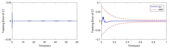
Figure 3. Tracking error of controller C1.

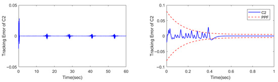
Figure 4. Tracking error of controller C2.

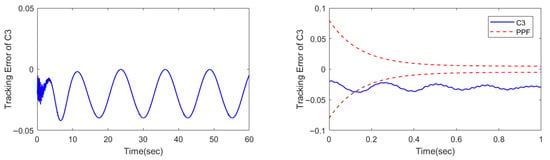
Figure 5. Tracking error of controller C3.

Specifically, due to the initial error set for the command signal, the tracking error does not start from 0 at the initial stage. This not only exerts a certain impact on the convergence performance of the controller but also reduces the steady-state tracking accuracy to a certain extent. However, as can be observed from the tracking error diagram and the locally enlarged view of the first 1 s, the C1 controller demonstrates better control performance both in terms of the error convergence speed at the initial stage and the steady-state tracking. Additionally, the convergence speed of the error existing at the initial stage falls within the set PPF range.

It can be seen from Figure 4 and Figure 5 that while the nonlinear controller C2 achieves relatively good convergence for the initial error, the model-free C3 controller shows much poorer tracking performance. Specifically, the C3 controller cannot eliminate the steady-state error, and its tracking error fluctuates within a certain range at all times. This further confirms the excellent tracking performance of the model-based control strategy, despite the complexity involved in its parameter tuning process.

According to Table 2, using the standard deviation of the tracking error as the evaluation criterion, the tracking control performance of the C1 controller is improved by 52.74% and 96.97% compared with that of the C2 and C3 controllers, respectively.

Table 2. Standard deviations of different controllers.

Controller	Standard Deviation	C1 − C2	C1 − C3
C1	4.059 × 10−4	52.74%	96.97%
C2	8.589 × 10−4
C3	1.340 × 10−2

In addition, the estimation results of the DESOs for matched and mismatched uncertainties can be observed in Figure 6, and actuator input in different controllers can be observed in Figure 7. Specifically, since the DESOs is designed to be combined with the system tracking error, the observation results also exhibit periodic fluctuations similar to the tracking error.

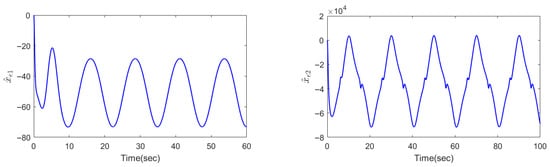
Figure 6. Disturbance compensation for matched and mismatched uncertainties.

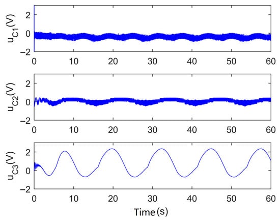
Figure 7. Control input of different controllers.

Combined with Figure 3 and Figure 4, the C1 controller with DESOs achieves better tracking performance compared with the C2 controller without DESOs. This advantage is reflected not only in the suppression of disturbances at the initial stage but also in the error convergence rate.

6. Contributions

This study effectively integrates PPF, DESOs, and RISE, providing a new method and approach for the high-precision tracking control of electro-hydraulic servo systems. Among them, PPF is mainly used to effectively suppress the initial error range and accelerate the convergence rate under the condition that the electro-hydraulic servo system has initial errors due to multi-sensor measurement, thus avoiding system instability. In addition, DESOs are mainly used for online observation of the matched and mismatched uncertainties existing in the system, and the observation results are integrated into the controller design process, enabling the controller to have active anti-disturbance capability and improving system stability. Finally, RISE is responsible for realizing the tracking control of the command signal, and the controller gains strong robustness by introducing an integral term. The specific process is shown in Figure 2.

7. Conclusions

Achieving high-precision position control is more difficult for electro-hydraulic servo systems than for motor-driven systems, primarily owing to their strong nonlinearity and unmodeled uncertainties. The main factor behind this challenge is that electro-hydraulic servo systems depend on multiple external sensing elements to acquire system state feedback, including position, pressure, and flow sensors. To address the demand for high-precision position tracking control, a robust integral of the sign of the error (RISE) control strategy integrated with a prescribed performance function (PPF) and dual extended state observers (DESOs) is proposed in this study. Designed based on the system dynamic model, the DESOs are utilized to estimate matched and mismatched uncertainties separately. Meanwhile, the prescribed performance function (PPF) is employed to derive the transformed error signal, which also serves to constrain the error’s convergence rate and range. Leveraging the backstepping approach, a RISE controller is developed to suppress both types of uncertainties and enhance the system’s robustness.

For application scenarios with initial system errors, where the system with single-rod hydraulic cylinders suffers from poor control accuracy and slow error convergence, the main work of this study is as follows:

• A PPF is first designed to convert the tracking error into a transformed error signal. This signal is then used to design the controller, ensuring that the convergence speed of the initial error remains within the set range and preventing excessive chattering and instability.
• DESOs are designed by integrating a system dynamics model. By selecting an appropriate observer bandwidth, online observation of both matched and mismatched uncertainties existing in the system can be achieved. This enables the subsequently designed control law to realize active compensation for these uncertainties, thereby improving control accuracy.
• Next, a RISE controller is designed using the observation results of the DESOs. By suppressing the disturbance observation error, the system achieves strong robustness. The tracking stability of the system is proven using the Lyapunov stability theory.
• Finally, by comparing with controllers that do not use PPF and DESOs, it is verified that the designed PPF-DESOs-RISE control strategy exhibits excellent tracking performance, with the tracking error remaining within the preset convergence range.

Through the systematic analysis of this study, the proposed method has effectively improved the tracking performance of the electro-hydraulic servo system under multiple disturbances, providing a new approach for its high-precision tracking control. However, due to the limitations of experimental conditions, it is impossible to conduct experimental tests to further verify its performance. In the future, efforts will be made to improve the experimental platform and realize the verification tests under experimental conditions.

References

- Li, J.F.; Ji, R.H.; Liang, X.L.; Ge, S.S.; Yan, H. Command Filter-Based Adaptive Fuzzy Finite-Time Output Feedback Control of Nonlinear Electrohydraulic Servo System. IEEE Trans. Instrum. Meas. 2022, 71, 3529410. [Google Scholar] [CrossRef]
- Lindh, P.; Tiainen, J.; Grönman, A.; Turunen-Saaresti, T.; Di, C.; Laurila, L.; Scherman, E.; Handroos, H.; Pyrhönen, J. Two Cooling Approaches of an Electrohydraulic Energy Converter For Non-Road Mobile Machinery. IEEE Trans. Ind. Appl. 2023, 59, 736–744. [Google Scholar] [CrossRef]
- Deng, W.X.; Yao, J.Y. Asymptotic Tracking Control of Mechanical Servosystems With Mismatched Uncertainties. IEEE/ASME Trans. Mechatron. 2021, 26, 2204–2214. [Google Scholar] [CrossRef]
- Akeila, E.; Salcic, Z.; Swain, A. Reducing Low-Cost INS Error Accumulation in Distance Estimation Using Self-Resetting. IEEE Trans. Instrum. Meas. 2014, 63, 177–184. [Google Scholar] [CrossRef]
- Xu, Z.B.; Sun, C.B.; Hu, X.L.; Liu, Q.Y.; Yao, J.Y. Barrier Lyapunov Function-Based Adaptive Output Feedback Prescribed Performance Controller for Hydraulic Systems With Uncertainties Compensation. IEEE Trans. Ind. Electron. 2023, 70, 12500–12510. [Google Scholar] [CrossRef]
- Liu, Z.; Zhao, Y.; Zhang, O.Y.; Gao, Y.B.; Liu, J.X. Adaptive fuzzy neural network-based finite time prescribed performance control for uncertain robotic systems with actuator saturation. Nonlinear Dyn. 2024, 112, 12171–12190. [Google Scholar] [CrossRef]
- Yao, Y.; Tan, J.Q.; Yao, Y.G.; Zhang, X.; Chen, P. Prescribed-time prescribed performance control for stochastic nonlinear input-delay systems with arbitrary bounded initial error. Neurocomputing 2024, 571, 127200. [Google Scholar] [CrossRef]
- Guo, Q.; Zhang, Y.; Celler, B.G.; Su, S.W. Neural Adaptive Backstepping Control of a Robotic Manipulator With Prescribed Performance Constraint. IEEE Trans. Neural Netw. Learn. Syst. 2019, 30, 3572–3583. [Google Scholar] [CrossRef]
- Zeng, Q.L.; Jia, B.Y.; Zhao, J.; Lv, Y.F.; Wan, L.R.; Meng, Z.S. Adaptive Learning-Based Optimal Prescribed Performance Tracking Error Measurement of Hydraulic Support Initial Support Force. IEEE Trans. Instrum. Meas. 2025, 74, 3515214. [Google Scholar] [CrossRef]
- Wang, C.W.; Jiao, Z.X.; Wu, S.; Shang, Y.X. Nonlinear adaptive torque control of electro-hydraulic load system with external active motion disturbance. Mechatronics 2014, 24, 32–40. [Google Scholar] [CrossRef]
- Li, Q.L.; Chang, X.H. Observer-based improved event-triggered interval type-2 fuzzy networked control systems subject to deception attacks in dual communication channels. Commun. Nonlinear Sci. Numer. Simul. 2025, 142, 108579. [Google Scholar] [CrossRef]
- Sarkar, A.; Maji, K.; Chaudhuri, S.; Saha, R.; Mookherjee, S.; Sanyal, D. Actuation of an electrohydraulic manipulator with a novel feedforward compensation scheme and PID feedback in servo-proportional valves. Control Eng. Pract. 2023, 135, 105490. [Google Scholar] [CrossRef]
- Zhao, G.Y.; Yang, X.W.; Deng, W.X.; Lu, C.J.; Yao, J.Y. Command-Filter-Based Velocity-Free Tracking Control of an Electrohydraulic System with Adaptive Disturbance Compensation. Mathematics 2025, 13, 3081. [Google Scholar] [CrossRef]
- Feng, H.; Yin, C.B.; Cao, D.H. Trajectory Tracking of an Electro-Hydraulic Servo System With an New Friction Model-Based Compensation. IEEE/ASME Trans. Mechatron. 2023, 28, 473–482. [Google Scholar] [CrossRef]
- Tian, D.P.; Xu, Q.; Yao, X.H.; Zhang, G.N.; Li, Y.F.; Xu, C.H. Diversity-guided particle swarm optimization with multi-level learning strategy. Swarm Evol. Comput. 2024, 86, 101533. [Google Scholar] [CrossRef]
- Gong, C.; Zhou, N.R.; Xia, S.H.; Huang, S.Y. Quantum particle swarm optimization algorithm based on diversity migration strategy. Future Gener. Comput. Syst. 2024, 157, 445–458. [Google Scholar] [CrossRef]
- Do, P.; Nguyen, V.; Voisin, A.; Iung, B.; Neto, W.A.F.; Neto, F. Multi-agent deep reinforcement learning-based maintenance optimization for multi-dependent component systems. Expert Syst. Appl. 2024, 245, 123144. [Google Scholar] [CrossRef]
- Mnih, V.; Kavukcuoglu, K.; Silver, D.; Rusu, A.A.; Veness, J.; Bellemare, M.G.; Graves, A.; Riedmiller, M.; Fidjeland, A.K.; Ostrovski, G.; et al. Human-level control through deep reinforcement learning. Nature 2015, 518, 529–533. [Google Scholar] [CrossRef]
- Coskun, M.Y.; Itik, M. Intelligent PID control of an industrial electro-hydraulic system. ISA Trans. 2023, 139, 484–498. [Google Scholar] [CrossRef]
- Chen, J.B.; He, G.; Wang, Y.H.; Zheng, Y.; Xiao, Z.H. Adaptive PID Control for Hydraulic Turbine Regulation Systems Based on INGWO and BPNN. Prot. Control Mod. Power Syst. 2024, 9, 126–146. [Google Scholar] [CrossRef]
- He, J.H.; Su, S.J.; Wang, H.R.; Chen, F.; Yin, B.J. Online PID Tuning Strategy for Hydraulic Servo Control Systems via SAC-Based Deep Reinforcement Learning. Machines 2023, 11, 593. [Google Scholar] [CrossRef]
- Yao, J.Y.; Deng, W.X.; Sun, W.C. Precision Motion Control for Electro-Hydraulic Servo Systems With Noise Alleviation: A Desired Compensation Adaptive Approach. IEEE/ASME Trans. Mechatron. 2017, 22, 1859–1868. [Google Scholar] [CrossRef]
- Yang, G.C.; Yao, J.Y.; Le, G.G.; Ma, D.W. Adaptive integral robust control of hydraulic systems with asymptotic tracking. Mechatronics 2016, 40, 78–86. [Google Scholar] [CrossRef]
- Chen, Z.; Zhou, S.Z.; Shen, C.; Lyu, L.; Zhang, J.H.; Yao, B. Observer-Based Adaptive Robust Precision Motion Control of a Multi-Joint Hydraulic Manipulator. IEEE/CAA J. Autom. Sin. 2024, 11, 1213–1226. [Google Scholar] [CrossRef]
- Zhu, Y.K.; Qiao, J.Z.; Guo, L. Adaptive Sliding Mode Disturbance Observer-Based Composite Control With Prescribed Performance of Space Manipulators for Target Capturing. IEEE Trans. Ind. Electron. 2019, 66, 1973–1983. [Google Scholar] [CrossRef]
- Deng, W.X.; Yao, J.Y. Extended-State-Observer-Based Adaptive Control of Electrohydraulic Servomechanisms Without Velocity Measurement. IEEE/ASME Trans. Mechatron. 2020, 25, 1151–1161. [Google Scholar] [CrossRef]
- Zhu, W.W.; Jia, M.W.; Zhang, Z.J.; Liu, Y. Dynamic data reconciliation for enhancing the performance of kernel learning soft sensor models considering measurement noise. Chemom. Intell. Lab. Syst. 2024, 246, 105083. [Google Scholar] [CrossRef]
- Deng, W.X.; Zhou, H.; Zhou, J.; Yao, J.Y. Neural Network-Based Adaptive Asymptotic Prescribed Performance Tracking Control of Hydraulic Manipulators. IEEE Trans. Syst. Man Cybern. Syst. 2023, 53, 285–295. [Google Scholar] [CrossRef]
- Mi, J.J.; Deng, W.X.; Yao, J.Y.; Liang, X.L. Linear-Extended-State-Observer-Based Adaptive RISE Control for the Wrist Joints of Manipulators with Electro-Hydraulic Servo Systems. Electronics 2024, 13, 1060. [Google Scholar] [CrossRef]
- Yang, G.C.; Zhu, T.; Yang, F.B.; Cui, L.F.; Wang, H. Output feedback adaptive RISE control for uncertain nonlinear systems. Asian J. Control 2023, 25, 433–442. [Google Scholar] [CrossRef]
- Mi, J.J.; Yao, J.Y.; Deng, W.X. Adaptive RISE Control of Winding Tension with Active Disturbance Rejection. Chin. J. Mech. Eng. 2024, 37, 52–64. [Google Scholar] [CrossRef]
Disclaimer/Publisher’s Note: The statements, opinions and data contained in all publications are solely those of the individual author(s) and contributor(s) and not of MDPI and/or the editor(s). MDPI and/or the editor(s) disclaim responsibility for any injury to people or property resulting from any ideas, methods, instructions or products referred to in the content. |
© 2025 by the authors. Licensee MDPI, Basel, Switzerland. This article is an open access article distributed under the terms and conditions of the Creative Commons Attribution (CC BY) license (https://creativecommons.org/licenses/by/4.0/).