Article

Control Crisis in Financial Systems with Dynamic Complex Network Approach

Centro Universitario de Ciencias Exactas e Ingenierías (CUCEI), Universidad de Guadalajara, Blvd. Marcelino Garcia Barragan 1421, Col. Olimpica, Guadalajara 44430, Jalisco, Mexico
*
Authors to whom correspondence should be addressed.
Mathematics 2025, 13(24), 3922; https://doi.org/10.3390/math13243922
Submission received: 31 October 2025 / Revised: 25 November 2025 / Accepted: 28 November 2025 / Published: 8 December 2025

Abstract

Financial stability in interconnected markets is increasingly challenged by nonlinear interactions that amplify local disturbances into systemic crises. This study models a financial system as a complex network of coupled chaotic nodes, where each node represents a nonlinear macroeconomic subsystem governed by endogenous feedback dynamics. In contrast to traditional centralized interventions, a pinning control strategy is proposed to stabilize a network through selective control of a small subset of influential nodes. Numerical simulations show how local crises propagate through coupling links, generating systemic instability, and how the proposed impulsive control scheme effectively suppresses chaos and restores synchronization across an entire network. Results highlight the efficiency of localized interventions for achieving global stability, offering new theoretical insights into mechanisms of financial correlation and design of control-based resilience strategies for complex economic systems.

1. Introduction

The contemporary global economy operates within an intricate web of interdependencies, rendering it increasingly vulnerable to systemic disturbances. Recent crises have shown that financial instability rarely emerges in isolation; instead, it arises from complex feedback loops linking markets, institutions, and national economies into dynamically coupled networks. Global Risks Report 2025 warns of a fragmented and highly interconnected landscape where multiple economic and social shocks—so-called polycrises—amplify one another through nonlinear interactions between financial and real sectors [1].
Financial systems can thus be understood as nonlinear dynamical networks in which each node represents an economic subsystem—such as a market, financial institution, or national economy—interacting through nonlinear feedback mechanisms. Within specific parameter variations, these systems may display chaotic oscillations in variables such as interest rate, investment demand, and price index, leading to endogenous instability and potential crises [2,3,4]. Propagation of such instability through interlinked agents defines global financial crises, reflecting endogenous coupling and correlation dynamics among economies [5].
Traditional regulatory and control approaches often rely on centralized, continuous, and global supervision of financial systems. However, these strategies are economically costly and structurally inefficient in large, interconnected networks. Their inability to address distributed and nonlinear properties of modern finance has motivated exploration of localized control frameworks inspired by complex systems theory. Within this context, pinning control offers an efficient and mathematically grounded approach for stabilizing large-scale nonlinear networks through interventions limited to a small subset of influential nodes [6,7].
Pinning control operates under a principle that stability can be achieved by acting on strategically selected nodes—so-called pinned nodes—whose structural centrality enables diffusion of corrective effects across interconnected subsystems. This concept aligns with real-world financial regulation, where targeted interventions—such as liquidity injections, interest rate adjustments, or macroprudential policies—are selectively applied to key institutions or markets to mitigate systemic risk [8,9,10].
From a theoretical perspective, pinning control integrates principles from nonlinear dynamics, synchronization theory, and Lyapunov stability analysis to design feedback mechanisms capable of restoring equilibrium in chaotic or stochastic environments [6,11]. When applied to financial networks, this approach bridges mathematical control theory and macroeconomic stability analysis, displaying that global stabilization can emerge from partial and discrete control actions rather than continuous full-network regulation.
Building on these foundations, this study extends the Gao–Ma nonlinear financial model [4] into a multi-node network representation of interconnected economies. By incorporating both stable and chaotic subsystems, the model reproduces heterogeneous and correlation-prone characteristics of real-world financial structures. A proposed impulsive pinning control strategy introduces discrete corrective interventions on a limited set of key nodes, emulating policy actions such as periodic monetary adjustments or emergency interventions during crisis periods.
The main contribution of this research lies in that global controllability and synchronization of chaotic financial networks can be achieved through localized, energy-efficient interventions, ensuring system-wide stability even when crises originate from a small subset of nodes. Numerical simulations validate this hypothesis, confirming that transitions from chaotic to stable regimes can be induced through impulsive control, thereby providing a quantitative foundation for resilient financial governance.

2. Theoretical Framework for Nonlinear Financial Networks

This section provides a theoretical foundation for modeling and controlling crisis propagation in nonlinear financial networks, serving as an analytical basis for stabilization methodology developed in Section 3. The goal is to establish a mathematical and conceptual framework linking macroeconomic dynamics, network theory, and control systems, enabling systematic study of how localized perturbations can escalate into global financial instability.
Modern financial systems are inherently nonlinear and interconnected, exhibiting dynamic behaviors ranging from equilibrium to chaos. Understanding such behaviors requires a formal framework integrating concepts from complex network theory, nonlinear dynamics, and control theory to describe and predict onset of instability.
Financial interactions among institutions, sectors, or national economies can be modeled as interdependent nodes connected through credit, trade, or liquidity relationships. Perturbations in one part of a system can propagate through feedback loops, amplifying volatility and leading to systemic crises. Such networked structures illustrate how small shocks may generate large-scale effects, as observed in cascading failures across global markets [3,5].
Following sections formalize this theoretical basis. Section 2.1 introduces concepts of complex financial networks and mathematical representation of interconnected agents. Section 2.2 examines nonlinear dynamic behavior of financial subsystems and emergence of chaos, while Section 2.3 explores principles of synchronization and controllability relevant to collective stability. Section 2.4, Section 2.5, Section 2.6, Section 2.7 extend these ideas to the Gao–Ma financial model [4], including dynamic classification, parameterization, and networked formulation.
Building upon these general concepts, this Section shows how chaotic economic dynamics can be represented as coupled nonlinear systems, providing a rigorous foundation for control strategies developed later to mitigate crisis propagation and restore macroeconomic stability.

2.1. Complex Networks and Financial Interconnectedness

A modern financial system can be represented as a complex network G = ( V , E ) , where V = { 1 , , N } denotes a set of nodes representing markets, institutions, or national economies; E V × V defines a set of edges capturing credit relations, asset exposures, or correlation channels; A = [ a i j ] { 0 , 1 } N × N is an adjacency matrix, where a i j = 1 if node i is connected to node j; and a i j = 0 . Otherwise, D = diag ( d 1 , , d N ) is a degree matrix with d i = j a i j and L = D A denotes a Laplacian matrix encoding diffusive coupling structure.
Network abstraction enables modeling how local perturbations—such as liquidity shocks or institutional defaults—propagate and amplify through interconnected agents, reproducing empirical patterns of systemic risk and financial correlation [3,5]. This representation aligns with World Economic Forum’s perspective on polycrisis interdependence among global systems [1].

2.2. Nonlinear Dynamics and Chaos in Economic Systems

Let X i ( t ) R d denote a state vector of node i, representing local macroeconomic variables. Its nonlinear evolution can be expressed as
X ˙ i = f ( X i ; θ i ) ,
where f : R d R d defines a local dynamic law; θ i denotes a parameter vector of node i (elasticities, frictions, or price rigidities).
Small variations in θ i or initial conditions may induce bifurcations and chaotic oscillations, as commonly observed in empirical time series of interest rates, investments, and prices [2]. Degree of chaos can be quantified through the largest Lyapunov exponent λ max , as follows:
  • λ max > 0 : trajectories diverge exponentially → chaotic regime [11];
  • λ max < 0 : trajectories converge → stable regime [11].
It is important to note that each isolated node modeled by (1) can independently display chaotic, quasi-periodic, or periodic dynamics, depending of system parameters. Such intrinsic nonlinear behavior is considered for each node’s dynamics and is affected by network coupling constituting a fundamental property of complex nonlinear systems, in this paper each node’s dynamics are defined by the Gao–Ma financial system [4], as explained in the next section.

2.3. Synchronization and Controllability in Complex Systems

When nodes interact, collective dynamics may exhibit synchronization, cluster formation, or asynchronization depending on coupling strength and network topology. A standard diffusive coupling form is
X ˙ i = f ( X i ) + σ j = 1 N a i j ( X j X i ) ,
where σ > 0 denotes coupling strength between nodes; a i j are elements of adjacency matrix A.
Large-scale global control acting simultaneously on all nodes is often economically impractical. Pinning control, in contrast, applies control inputs only to a subset of nodes—referred to as pinned nodes—whose structural influence enables desired dynamics to propagate across network [6,7].
Robust and stochastic formulations extend this approach to uncertain or time-varying topologies, preserving convergence guarantees even under random perturbations [8].

2.4. Transition from Chaotic Behavior to Stabilization

Transition from chaotic to stable behavior in nonlinear networks depends on three key design elements:
  • Network structure—coupling topology and connection weights;
  • Pinned node selection—identification of nodes receiving control;
  • Feedback design—continuous, impulsive, or adaptive schemes.
This process relies on Lyapunov stability theory, bifurcation analysis, and optimization criteria that minimize control energy while guaranteeing global convergence [6,7,11]. Contemporary approaches optimize sets of pinned nodes using network-theoretic or machine-learning-based algorithms, reducing both intervention frequency and implementation cost [9,10,12].

2.5. Gao–Ma Nonlinear Financial System

As foundation for applied model, Gao–Ma nonlinear financial system [4] describes interactions among interest rate x, investment demand y, and price index z:
x ˙ = z + ( y a ) x , y ˙ = 1 b y x 2 , z ˙ = x c z .
where x represents interest rate, y is investment demand, z is price index, a > 0 is liquidity or saving propensity, b > 0 is damping coefficient in investment adjustment, c > 0 defines price rigidity. System dynamics vary according to parameters a, b, and c. Bifurcation analyses indicate the following: 0 < a 6.42 and 6.61 < a 7.02 : chaotic regime (unstable crisis-like behavior), 6.41 < a 6.60 and 7.03 < a 7.09 : quasi-periodic or toroidal regime, 7.10 < a 8.94 : periodic cycles, 8.95 < a 10 : stable steady state. Hence, smaller values of a correspond to financial fragility and crisis emergence [2,4].

2.6. Extension to Financial Networks

To represent systemic interdependence, local Gao–Ma dynamics can be extended to a network of N nodes, where each node evolves as
x ˙ i = z i + ( y i a i ) x i + σ j = 1 N a i j ( x j x i ) , y ˙ i = 1 b y i x i 2 , z ˙ i = x i c z i ,
with a i defined as saving parameter of node i (heterogeneous across agents), σ > 0 coupling strength, A = [ a i j ] adjacency matrix of financial connections.
This formulation enables analysis of correlation, stability, and systemic propagation, aligning with recent studies on network-based systemic risk modeling [3,5].

2.7. Simulation of Heterogeneous Macroeconomic Conditions

To simulate heterogeneous macroeconomic conditions, in this paper, it is considered a 12-node network with the following topology:
  • Nodes 1–8: a i [ 7.10 , 8.94 ] → stable or periodic economies.
  • Nodes 9–10: a i ( 6.41 , 6.60 ] → vulnerable economies.
  • Nodes 11–12: a i [ 6.00 , 7.02 ] → chaotic or crisis economies.
This configuration reproduces a financial ecosystem combining resilient, fragile, and crisis-prone agents. Through coupling and diffusion (A and σ ), local instability can propagate across global systems, motivating control strategies developed in the next section [3].
In summary, pinning control provides a robust theoretical framework for achieving stability in large-scale complex systems through partial and strategically localized interventions. Rather than applying continuous global regulation—often infeasible or economically inefficient—pinning control shows that stabilization can be accomplished by influencing only a subset of critical nodes whose connectivity enables corrective effects to propagate across entire networks [6,7].
This concept carries strong implications for economic and financial systems, where localized policy actions—such as targeted monetary adjustments, liquidity injections, or macroprudential regulations—can restore global stability without requiring universal intervention. Essentially, it bridges nonlinear dynamics and macroeconomic governance, illustrating how selective measures can prevent systemic collapse and sustain equilibrium under crisis conditions [3,5].
The following section applies this control paradigm to a nonlinear financial network model, displaying how strategic pinning interventions can mitigate systemic crises, synchronize chaotic subsystems, and recover collective stability across interconnected economies.

3. Pinning Control for Financial Systems Under Crisis

Stability of global financial systems under crisis conditions represents one of the most challenging frontiers in nonlinear control theory. Viewing economies as interconnected nonlinear and chaotic networks, where each node corresponds to an economic subsystem—such as a market, financial institution, or national economy—enables identification of how targeted interventions can suppress systemic instability through localized control actions. Within specific parameter ranges, these systems may exhibit chaotic fluctuations in key macroeconomic variables such as interest rate, investment demand, and price index, which can evolve into systemic crises through correlation effects [2,3,4].
Propagation of instability across interconnected agents constitutes a defining feature of global financial crises, reflecting endogenous coupling among economies [5]. When subsystems exceed stability thresholds, global control strategies—analogous to continuous large-scale regulation—become impractical or economically inefficient, requiring simultaneous intervention across all components and involving prohibitive implementation costs.
In contrast, pinning control emerges as a selective and energy-efficient alternative, stabilizing entire networks by acting only on a limited subset of strategically influential nodes, known as pinned nodes, whose structural influence enables diffusion of corrective dynamics throughout interconnected systems [6,7,8]. This mechanism parallels real-world financial regulation, where discrete interventions—such as liquidity injections, reserve adjustments, or policy rate modifications—are selectively applied to stabilize systemic behavior through key institutions or markets.
The objective of this section is to formalize the application of pinning control theory to a nonlinear financial network, extending classical Gao–Ma model [4] into an interconnected macroeconomic framework. Section 3.1 introduces mathematical formulation of each node’s dynamics. Section 3.2 defines selection and role of pinned nodes, followed by stability and controllability conditions analyzed in Section 3.3 using Lyapunov theory. Finally, Section 3.4 outlines methodological implementation and simulation procedures employed to validate proposed impulsive control strategy. This formulation bridges nonlinear dynamics and financial stability analysis, providing a quantitative foundation for exploring how localized regulatory actions can produce global stabilization under crisis conditions.

3.1. Fundamentals of Pinning Control

Stabilizing nonlinear financial systems during periods of economic turbulence requires robust control strategies capable of mitigating instability and synchronizing behavior of interconnected markets. Within complex network control, pinning control provides an efficient approach to achieving global stability by applying control inputs only to a small subset of nodes representing key financial agents or economies [6,8,13]. In general, a controlled complex network with N interacting nodes can be described as
X ˙ i = F ( X i ) + c j = 1 N a i j H ( X j X i ) + b i U i ,
where X i R n represents state vector of node i, F ( X i ) denotes intrinsic nonlinear dynamics of node i, H ( X j X i ) defines coupling interaction between nodes i and j, a i j are elements of adjacency matrix A, defining financial interconnections among institutions or markets, c > 0 is coupling strength and b i { 0 , 1 } indicates whether node i is directly influenced by external control input U i .
In this work, impulsive control gain is represented by scalar parameter b i , following the original formulation of Gao and Ma [4]. Since control action is applied to entire three-dimensional state vector X i = [ x i , y i , z i ] T through deviation X i X r , a single scalar gain uniformly rescales all components. Scalar pinning strategies are widely adopted in nonlinear impulsive control, where proportional vector rescaling suffices to induce synchronization without requiring full 3 × 3 gain matrices. This simplification aligns with prior impulsive synchronization studies [6,13,14].
The control objective is to minimize number of driven nodes while ensuring global synchronization and macroeconomic stability, even under volatility and correlation conditions [11].
In financial contexts, each node can represent a national economy or major institution, and control inputs correspond to policy interventions such as liquidity regulation, rate adjustment, or capital injection.
To model this scenario, general formulation in (5) is specialized to the nonlinear financial system originally proposed by Gao and Ma [4]. This model captures endogenous oscillations in interest rates, investment demand, and prices, reproducing transitions from stable equilibria to chaotic crises. Building on this foundation, subsequent sections develop mathematical formulation, coupling structure, and pinning control design enabling stabilization of financial networks under crisis conditions.
Consider a financial network composed of N interconnected nodes, where each node i represents a financial subsystem governed by the nonlinear dynamics introduced by Gao and Ma [4]:
x ˙ i = z i + ( y i a i ) x i , y ˙ i = 1 b y i x i 2 , z ˙ i = x i c z i ,
where x i , y i , and z i denote the state variables of node i, representing, respectively, the following: x i represents interest rate associated with node i; y i is investment demand and z i is price index.
Derivatives x ˙ i , y ˙ i , and z ˙ i describe temporal evolution driven by nonlinear dynamics of Gao and Ma [4]. Parameters a i , b, and c define core macroeconomic sensitivities, with a i modeling responsiveness of interest rates to investment, b introduces damping in investment demand c quantifies price rigidity. System exhibits chaotic transitions as saving parameter a i decreases, while b = 0.1 and c = 1 remain constant. Equilibrium point is given by
( x , y , z ) = 0 , 1 b , 0 = ( 0 , 10 , 0 ) ,
Each financial subsystem described by the Gao–Ma model can be represented as a nonlinear node whose local stability is determined by the Jacobian matrix at equilibrium:
J = 10 a 0 1 0 0.1 0 1 0 1 .
As savings parameter a decreases, eigenvalues of J may cross the imaginary axis, producing Hopf bifurcations and leading to chaotic oscillations in macroeconomic variables [4]. Each node in a network is expressed as a vector:
X i = [ x i , y i , z i ] T R 3 ,
where x i , y i , and z i denote interest rate, investment demand, and price index of node i, respectively.
Its local nonlinear dynamics are summarized by f ( X i ) , while interconnections among financial agents are modeled by diffusive coupling:
X ˙ i = f ( X i ) + σ j = 1 N a i j ( X j X i ) ,
where σ > 0 denotes the coupling strength, A = [ a i j ] is the adjacency matrix of financial connections, with a i j = 1 if nodes i and j are connected and a i j = 0 otherwise.
Local perturbations in any node can propagate through coupling links, producing correlated fluctuations in investment, interest rate, or price levels across a network. To restore stability and steer a system toward a shared equilibrium, pinning control introduces selective feedback mechanisms acting only on a subset of nodes—known as pinned nodes—which serve as anchors for overall network dynamics [6,7,8]. Controlled network dynamics are thus represented as
X ˙ i = f ( X i ) + σ j = 1 N a i j ( X j X i ) g i ( X i X i , r ) ,
where g i corresponds to node i, referred to as a pinned node: g i = g > 0 for pinned nodes and g i = 0 otherwise X r = [ x r , y r , z r ] T defines reference state or equilibrium toward which synchronization is desired.
Control objective
X i ( t ) X i , r as t ,
meaning that all nodes converge asymptotically to the same reference trajectory, thereby achieving global synchronization across the financial network.

3.2. Optimal Selection of Pinning Nodes

Determining which nodes require control is formulated as a combinatorial optimization problem. The objective is to identify a minimal subset P { 1 , 2 , , N } that guarantees full synchronization.
A genetic algorithm (GA) encodes each possible configuration as a binary vector:
B = [ b 1 , b 2 , , b N ] , b i = 1 , if node i is pinned , 0 , otherwise .
Optimization fitness function aims to minimize global mean-squared synchronization error:
J = 1 N · d i = 1 N k = 1 d ( x i , k x r , k ) 2
where d = 3 denotes the system dimension (three variables per node), x i , k represents the k-th component of node i’s state vector, and x r , k corresponds to the reference component of the equilibrium X r = [ x r , y r , z r ] T . The evolutionary process proceeds through sequential stages:
  • Initialization: generation of a random population of candidate control configurations.
  • Evaluation: network dynamics are simulated to compute J and estimate Lyapunov exponents.
  • Selection and crossover: individuals exhibiting lower error are recombined to explore improved control strategies.
  • Convergence: the algorithm terminates once J stabilizes at a minimum or the largest Lyapunov exponent becomes negative ( λ max < 0 ), indicating a synchronized regime.
From an economic standpoint, nodes identified as pinned correspond to systemically critical institutions—banks or entities whose activity significantly influences global stability. Targeted intervention over such nodes acts as a focused regulatory policy, achieving systemic stabilization with minimal control effort and reduced resource expenditure.

3.3. Stability and Controllability Analysis

Stability analysis relies on an impulsive Lyapunov function defined as
V ( X ) = ( X X r ) P ( X X r ) ,
where V ( X ) is a continuously differentiable, positive-definite function measuring the deviation of the network state from the desired equilibrium X r . Here,
X = [ x 1 , y 1 , z 1 , , x N , y N , z N ] ,
denotes the global state vector of the financial network, X r = [ x r , y r , z r ] is the reference equilibrium point, and P R 3 N × 3 N represents a symmetric, positive-definite matrix used as a Lyapunov weighting matrix. During control-free intervals, the time derivative of V ( X ) satisfies
V ˙ ( t ) = ( X X r ) T ( A T P + P A ) ( X X r ) ,
where
A = f ( X ) X X = X r
is the Jacobian matrix of the linearized network dynamics evaluated around the equilibrium point X r . It is assumed to remain constant in the neighborhood of X r to ensure local exponential stability. Although the system is globally nonlinear, the Lyapunov analysis is conducted in a neighborhood of the equilibrium point, where the linearization via the Jacobian A is valid. Impulsive pinning forces trajectories to remain in this local region during stabilization, ensuring that the LMI-based stability conditions apply. At impulsive instants t k = k T , when the impulsive control is applied, the Lyapunov function experiences a discrete jump:
V ( t k + ) V ( t k ) = ( X ( t k ) X r ) T Q ( X ( t k ) X r ) ,
where Q = g T P g , and g R 3 N × 3 N is the control gain matrix, typically diagonal, indicating which nodes are subject to impulsive control (for uncontrolled nodes, g i = 0 ). The existence of matrices P , Q > 0 satisfying the Linear Matrix Inequality (LMI) conditions guarantees exponential stability for the impulsive dynamics. In other words, if the inequalities
A T P + P A < 0 , Q > 0 ,
with the Linear Matrix Inequality (LMI) conditions satisfied, network trajectories converge asymptotically to the reference state X r . The largest Lyapunov exponent λ i , max serves as the principal stability measure, obtained through the procedure of Wolf et al. [11], which estimates the exponential divergence of nearby trajectories in phase space.
λ i , max > 0 System exhibits chaotic behavior ,
λ i , max < 0 Network achieves synchronized and stable regime .
Once the impulsive pinning control is activated, the network transitions from a chaotic regime ( λ i , max > 0 ) to a synchronized and asymptotically stable regime ( λ i , max < 0 ), confirming the global controllability of the financial system and demonstrating the effectiveness of the proposed control scheme [6,8]. From a macroeconomic perspective, this result suggests that global financial stability can arise through localized and discrete interventions [2,3]. Comprehensive and continuous regulation of all agents becomes unnecessary; stabilization can instead be achieved by targeting key financial nodes whose interconnections disseminate corrective influence throughout the entire network [9].

3.4. Methodology

The methodological procedure of this research is based on nonlinear dynamic modeling, numerical simulation, and control techniques applied to complex networks. The starting point is the financial model proposed by Gao and Ma (2009) [4], recognized in the literature for its ability to represent the evolution of macroeconomic variables within an internally unstable environment and, therefore, adopted as the base structure for simulations in this study.

3.4.1. Use of Synthetic Data

It is important to note that, in this first stage of the research, all simulations are performed using synthetic data generated directly from the nonlinear Gao–Ma financial model [14]. This methodological decision is deliberate: the objective of the present study is to isolate and analyze the intrinsic dynamic behavior of the system—including bifurcations, chaos emergence, and stabilization through impulsive pinning control—without interference from exogenous noise, regime shifts, or measurement effects typically present in empirical financial time series. Using controlled synthetic data ensures a clean and reproducible evaluation of the proposed control strategy and supports methodological rigor when characterizing transitions between dynamic regimes. The incorporation of real financial data will be addressed in future work, once the methodological framework has been fully validated and extended to empirical financial networks.
To represent the interdependent nature of global markets, the mathematical model is extended to a network composed of twelve coupled nodes, where each node corresponds to a market or economy with its own financial dynamics. This approach aligns with recent studies showing that financial systems operate as complex networks with crisis correlation, in which instability of one node can propagate across the entire network [3,5]. In computational implementation, such a network is defined through an adjacency matrix representing financial connections among nodes, enabling simulation of systemic phenomena.

3.4.2. Choice of Network Topology

The choice of a scale-free topology for generating the adjacency matrix is intentional. Scale-free networks reproduce key structural properties of real financial and economic systems, including heterogeneous degree distributions, the presence of highly connected hubs, and robustness–fragility asymmetries. These features reflect the architecture of real markets, where a small number of systemically important institutions dominate the connectivity structure. Prior studies have reported that scale-free networks provide a more realistic representation of financial interactions than Erdős–Rényi or small-world topologies [15] and, thus, offer a suitable framework for studying crisis propagation and stabilization mechanisms.
A genetic algorithm identifies an optimal subset of pinned nodes, while impulsive pinning control ensures stability through localized interventions. Simulation results compare system behavior with and without control, evaluating the following:
  • Chaotic propagation under crisis conditions;
  • Stabilization after applying pinning control;
  • Reduction of global oscillations and Lyapunov exponents.
This methodological framework shows that financial stability can be achieved through discrete, targeted interventions rather than continuous regulation, reinforcing applicability of pinning control within real-world economic systems [2,5,9].

3.4.3. Dynamic Modeling of Financial System

Initial framework of this study relies on the nonlinear model proposed by Gao and Ma [4], which captures interactions among three fundamental macroeconomic variables: interest rate ( x i ), investment demand ( y i ), and price index ( z i ). This dynamic system represents internal evolution of a financial subsystem or individual economy i, defined by the following set of ordinary differential equations:
x ˙ i = z i + ( y i a i ) x i ,
y ˙ i = 1 b y i x i 2 ,
z ˙ i = x i c z i .
Although nodes share the same nominal parameters, chaotic behavior emerges from the nonlinear feedback term ( y i a i ) x i , which produces sensitive dependence on initial conditions. Even under homogeneous parameters, small perturbations in initial states generate divergent trajectories, leading to intrinsic chaos consistent with the Gao–Ma system’s structure.
In this formulation, dynamics are governed by three key parameters a i as saving propensity or sensitivity of economy i, b is damping factor in investment demand, acting as resistance to abrupt fluctuations and c: parameter associated with price rigidity, regulating market response to economic perturbations.
System behavior depends directly on parameter values, particularly a i . Resulting dynamics can be classified into distinct regimes according to the range of a i , as summarized in Table 1. These bifurcation ranges are verified numerically through continuation analysis and are consistent with previous studies on the Gao–Ma financial model [4], where transitions between stable, periodic, and chaotic regimes occur for similar values of the saving parameter a i .
Bifurcation intervals associated with parameter a i follow the original characterization reported by Gao and Ma [4], who demonstrated through numerical continuation that the system transitions from chaotic to periodic and eventually stable regimes as a i increases.
A reduction in a i induces unstable oscillations in macroeconomic variables—particularly interest rate and investment—typically associated with periods of financial crisis [2]. Conversely, higher a i values promote stable and predictable behavior, characteristic of resilient economies.
Model Nomenclature
To facilitate understanding of financial system and its extensions to complex networks, following nomenclature summarizes variables and parameters used in Equations (19)–(21) and Table 2.
Based on this conceptual and formal foundation, subsequent subsections extend the individual model into a complex financial network of multiple interconnected economies, incorporating structural heterogeneity and later introducing impulsive control strategies.

3.4.4. Extension to Dynamic Financial Networks

Within interconnected global markets, financial systems cannot be analyzed as isolated entities. Each economy or financial institution remains linked to others through relationships of credit, investment, or shared risk. To capture such structural interdependence, the nonlinear Gao–Ma model [4] is extended into a financial network composed of N nodes, where each node represents a local economy with its own macroeconomic dynamics.
Connections among nodes are defined by an adjacency matrix A = [ a i j ] , whose elements indicate the presence or absence of financial relationships between nodes i and j:
a i j = 1 , if a financial relationship exists between nodes i and j , 0 , otherwise .
Each node preserves nonlinear equations from the original model but now receives influences from connected counterparts. Accordingly, the evolution of interest rate incorporates a diffusive coupling term representing financial correlation among entities:
x ˙ i = z i + ( y i a i ) x i + ε j = 1 N a i j ( x j x i ) ,
while other variables maintain their original structure:
y ˙ i = 1 b y i x i 2 ,
z ˙ i = x i c z i .
In these equations:
  • ε > 0 denotes coupling intensity, expressing degree of financial correlation or mutual economic influence among nodes;
  • the term j = 1 N a i j ( x j x i ) quantifies differences in interest rates across connected nodes;
  • weighted sum defined by matrix A determines how local fluctuations propagate across network.
This network formulation realistically captures mechanisms of financial correlation, enabling analysis of how localized disturbances may amplify and evolve into systemic crises [3].

3.4.5. Heterogeneous Financial Network Configuration

To more accurately represent heterogeneity across global economies, each pair of nodes i is assigned a distinct value of savings parameter a i , determining its specific dynamic behavior. Parameter distribution reflects the coexistence of stable, vulnerable, and crisis-prone economies within a single interconnected system.
Assignment of a i values for twelve nodes used in simulation appears in Table 3.
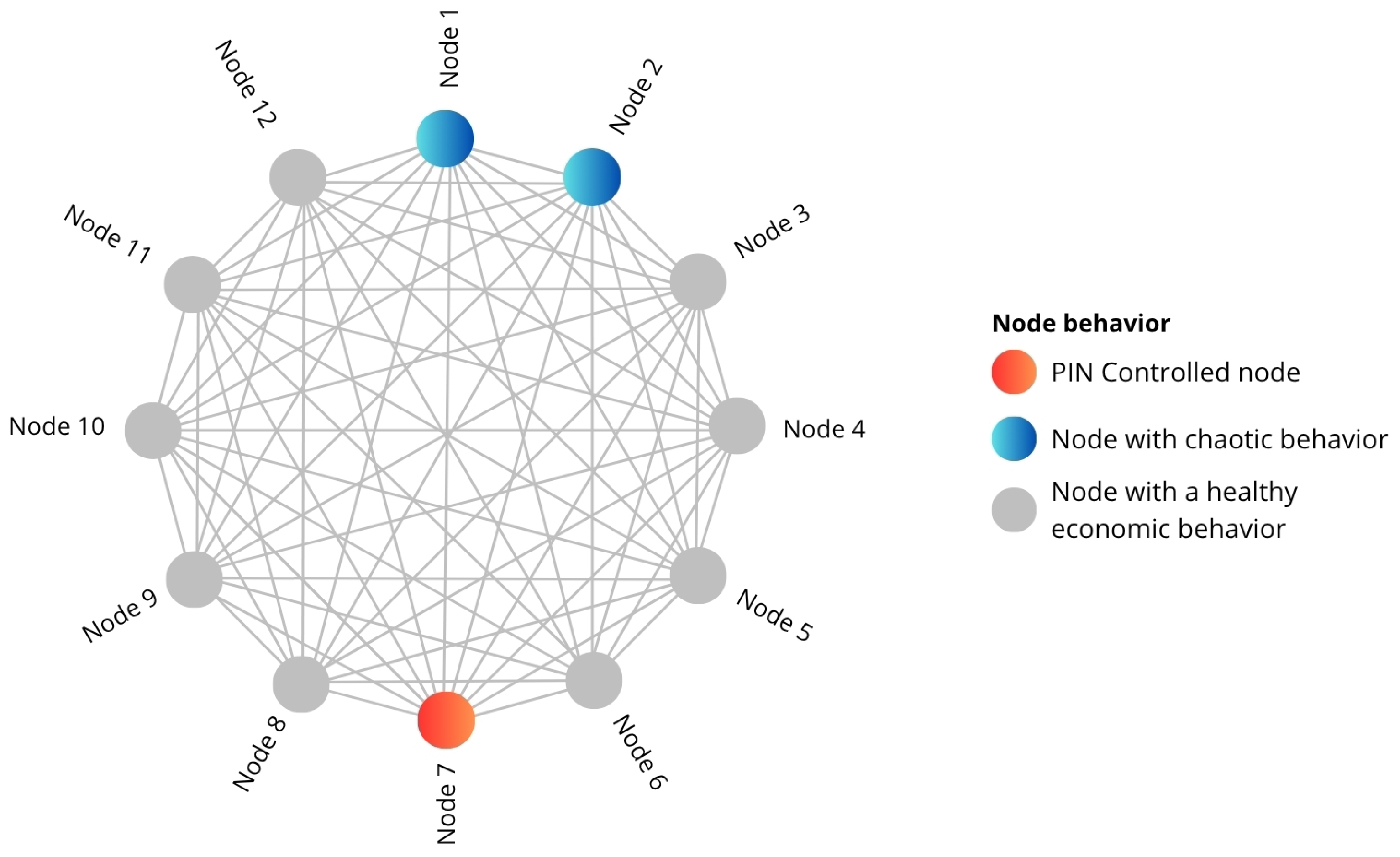
This configuration is deliberately asymmetric, allowing chaotic behavior to originate locally (nodes 1 and 2) while retaining potential to spread across network through financial connections. Such setup is crucial for analyzing crisis propagation phenomena, as it reproduces realistic scenarios where disturbances emerge within weak economies and later expand on a global scale. Setup is illustrated in Figure 1. In all numerical results, the adjacency matrix is generated according to a scale-free mechanism so that node degrees follow a heavy-tailed distribution. This choice reflects empirical findings that real financial systems exhibit scale-free connectivity patterns, with a small number of highly connected institutions acting as hubs and many peripheral institutions with low degree. Such topologies have been shown to provide a better approximation of real-world networks than homogeneous Erdős–Rényi or regular structures [15], making scale-free networks a natural framework for modeling financial correlation and systemic risk.
Nodes later selected for impulsive control (pinned nodes) will be identified in subsequent figures.

3.5. Pinning Control with Impulsive Actions

Impulsive pinning control represents an efficient technique for stabilizing complex chaotic networks by applying discrete actions to a limited set of strategic nodes. Instead of employing continuous control—costly and impractical in economic contexts—this approach operates through periodic and localized interventions capable of inducing global synchronization across network coupling structures [6,9,13].
Relevance of this method lies in its analogy to real regulatory mechanisms: economies do not receive continuous control but rather targeted interventions such as monetary policies, bank bailouts, or liquidity injections that correct critical deviations without requiring permanent supervision [5].

3.5.1. Mathematical Formulation

Considering a coupled financial network of N nodes described in Section 3.4.4, impulsive control is applied at discrete time instants t k = k T , where T denotes interval between impulses. Between impulses, the system evolves freely following Gao and Ma’s nonlinear dynamics [4]. At each instant t k , a control term instantaneously adjusts the node state:
X i ( t k + ) = ( 1 g i ) X i ( t k ) + g i X r
where
X i = [ x i , y i , z i ] T R 3
is state vector of financial node i;
X r = [ x r , y r , z r ] T
represents reference equilibrium targeted for synchronization [6]; g i denotes control gain associated with node i, where g i = g > 0 for controlled nodes and g i = 0 otherwise. A scalar gain g i is employed instead of a matrix gain to ensure uniform impulsive strength across the three state variables of each node. This simplification preserves stability while reducing computational complexity, as supported by stability proofs for scalar impulsive controllers in multidimensional systems [16].
Superscripts ( ) and ( + ) mark instants immediately before and after impulse, respectively. This scheme proves effective in nonlinear networks, particularly under heterogeneous or stochastic configurations [8]. Control logic gradually reduces deviation
e i = X i X r ,
ensuring convergence of all nodes toward synchronized dynamics with minimal energy expenditure.

3.5.2. Economic Interpretation

From an economic standpoint, each node in the financial network represents an individual economy interacting with others through credit, investment, and liquidity relations. Parameter a i defines saving propensity or internal stability of each economy: smaller values correspond to speculative or crisis-prone markets, while larger ones indicate resilient and well-regulated economies. Coupling term ε j = 1 N a i j ( x j x i ) models financial correlation, expressing how fluctuations in interest rates or investment demand spread among interconnected economies. Control gain g i symbolizes strength of policy interventions such as liquidity injections or monetary adjustments, applied selectively to key nodes with high systemic influence. Under this framework, impulsive pinning control captures essence of real-world stabilization mechanisms—periodic and localized interventions capable of restoring macroeconomic equilibrium with minimal regulatory effort.

3.5.3. Impulsive Control Energy

Control performance is evaluated through accumulated impulse energy, quantifying total cost of interventions applied during simulation:
E c = k = 1 M g ( X ( t k ) X r ) 2 ,
where M denotes total number of impulses executed and · represents Euclidean norm.
Parameter E c reflects control efficiency: smaller values indicate stabilization achieved with lower energy expenditure or, in economic terms, reduced intervention cost [9,10]. Proper tuning of sampling period T and gain g enables simultaneous optimization of convergence speed and control cost, maintaining balance among stability, efficiency, and financial realism.

3.5.4. Advantages of Impulsive Approach

Theoretical and numerical results have shown that impulsive control provides significant advantages over continuous methods [6,7]: Energy efficiency: control activates only when deviation X i X r exceeds a critical threshold, avoiding unnecessary interventions. Structural robustness: control signals propagate through coupling links, allowing stabilizing effects of a few nodes to spread across network [8]. Financial realism: discrete nature of impulses more accurately reproduces dynamics of real economic decisions, where regulatory policies occur episodically and strategically [5].

3.5.5. Control Performance Evaluation

Synchronization and stability levels of a system are quantified through global mean-squared error, defined as
J = 1 N i = 1 N X i X r 2 .
Function J measures average deviation of all nodes from desired equilibrium X r . In economic terms, a sustained reduction in J corresponds to decreasing systemic volatility and transition toward a stable macroeconomic regime [9,11]. Goal of impulsive control is to minimize J by optimally selecting subset P { 1 , 2 , , N } of controlled nodes, ensuring global synchronization with minimal effort. In summary, impulsive pinning control represents a decentralized stabilization mechanism acting on influential nodes within a system, optimizing energy usage and reducing intervention costs. Its discrete structure, inspired by real financial market dynamics, makes this method a powerful tool for analyzing and managing systemic crises in complex economic networks [4,6,8,9].

4. Results

The analysis focuses on the system’s dynamic characteristics, particularly on how the network’s behavior evolves before and after applying control methods. Stability is evaluated through the Lyapunov spectrum, which measures whether small perturbations in the system amplify or decay over time. This assessment is based on simulations of a nonlinear financial system and a 12-node coupled complex network.

4.1. Dynamic Behavior of the Isolated System

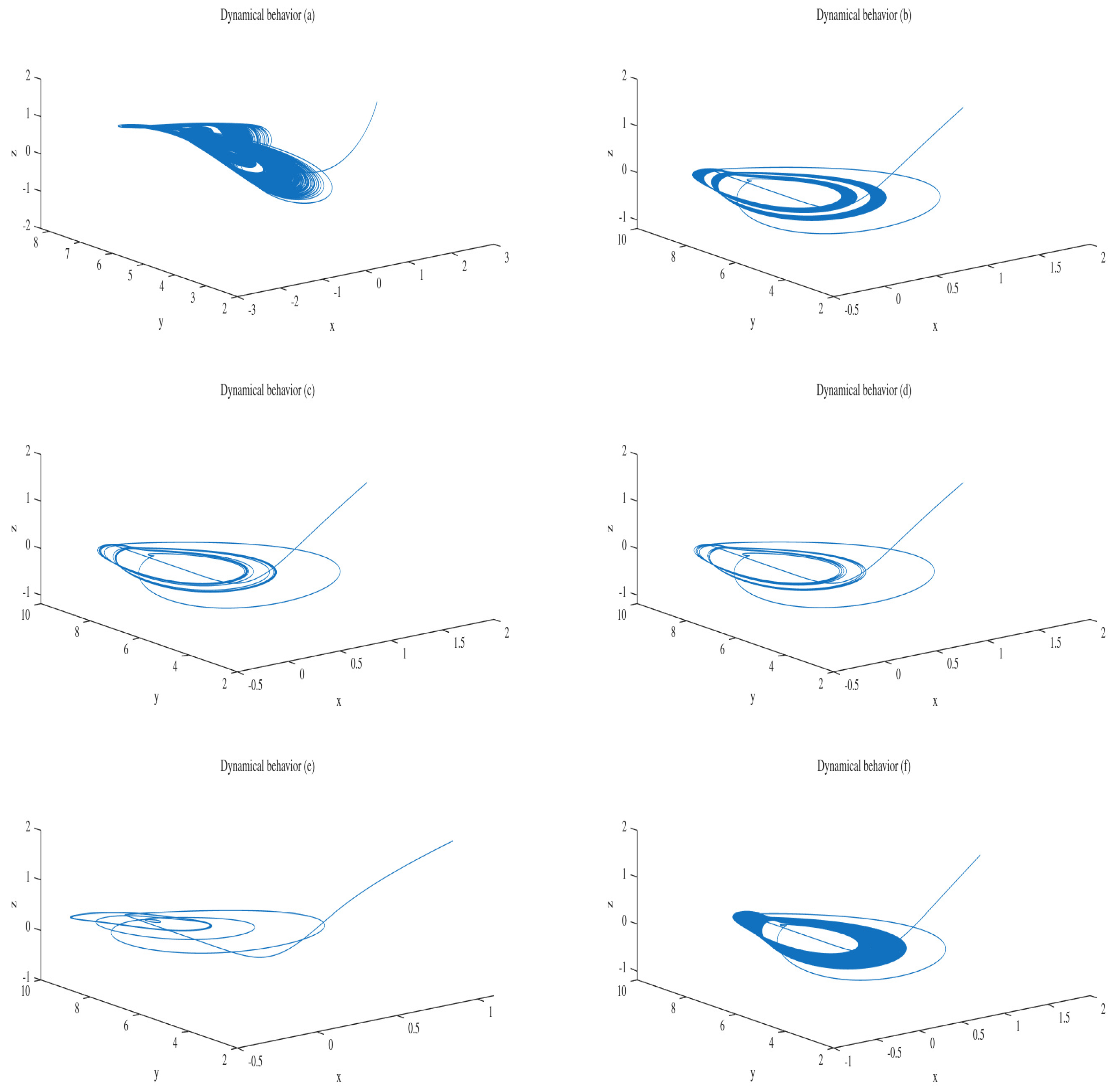
Figure 2 shows dynamic behavior of the proposed financial system, modeled after a Lorenz-type system adapted to macroeconomic variables: interest rate x ( t ) , investment demand y ( t ) , and price index z ( t ) . This model captures the nonlinear interactions and bifurcation phenomena that characterize unstable economic systems.
System exhibits chaotic behavior with irregular trajectories and high sensitivity to initial conditions when a i = 6 . As the value of a i increases to 7.07 and 7.15, the system transitions toward quasi-periodic regimes, displaying organized oscillations with moderate variability. For a i = 7.20 and a i = 8.30 , the dynamics stabilize into regular periodic cycles, whereas for a i = 7.03 , the system operates at the edge of chaos, showing intermittent oscillations between stability and instability.
These results confirm that parameter a i acts as a bifurcation factor regulating macroeconomic stability. Lower values of a i tend to induce chaotic dynamics associated with financial crises, while higher values promote periodic oscillations and stable regimes that represent balanced economic conditions.

4.2. Dynamic Behavior of the Controlled Financial Network

Chaos is observed in nodes 1 and 2 of the financial network, as described in Section 3.4.4, since they are configured with parameters corresponding to a chaotic regime. These nodes generate perturbations that propagate through the coupled connections to the rest of the network, resulting in a loss of synchrony and an amplification of fluctuations in the variables x, y, and z. Such behavior reproduces the phenomenon of financial correlation, a characteristic feature of systemic crises.
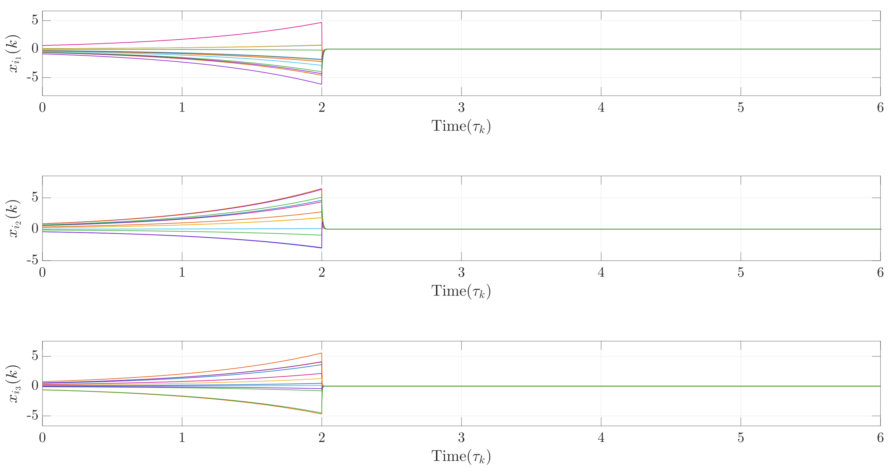
Figure 3 visually depicts the temporal evolution of the interconnected financial nodes, including the chaotic nodes and pin node, where the impulsive pinning control is applied.
Impulsive pinning control is applied to node 7 because the pin node is identified with a genetic algorithm as the most influential node within the network topology. The selection of this node allows for maximizing the global stabilization effect while acting only on a single element. Meanwhile, perturbations originating from nodes 1 and 2 continue to spread chaotic dynamics through the coupled links. In this configuration, node 7 functions as the pin node, transmitting the control signal to induce synchronization across the network and mitigating the propagation of financial chaos.
In this numerical example, the initial validation of the impulsive pinning control is conducted on a 12-node financial network, where node 7 is identified as the optimal pin node. The dynamic responses shown in Figure 3 and Figure 4 correspond to this 12-node configuration and serve as representative visualizations of the overall stabilization process.
To assess scalability and robustness, the same control strategy is extended to a 100-node network. In this larger configuration, the genetic algorithm identified nodes 11, 29, and 95 as the most influential, thus being selected as the control nodes. The results confirmed that the synchronization and stabilization patterns observed in the 12-node case remained consistent, with similar convergence behavior and global stabilization effects despite the increased network size. Therefore, the 12-node figures effectively illustrate the general dynamics representative of the 100-node system.
Figure 4 illustrates the temporal evolution of the complex financial network. At the beginning, the uncontrolled regime exhibits the spread of chaos across the nodes; however, once the impulsive pinning control is applied during the second iteration, the system progressively stabilizes.
These results show that even when a fraction of the nodes operate under a chaotic regime, economic interdependence tends to propagate instability toward otherwise stable economies, producing joint oscillations and a loss of structural resilience. Successful stabilization achieved through selection of optimal pin node highlights the importance of network topology in chaos containment, confirming that global stability can be attained with minimal control effort.

4.3. Scalability and Network Connectivity Analysis

To evaluate scalability and robustness of the proposed impulsive pinning control strategy, simulations are extended to networks of N = 100 nodes under different connectivity levels. Each configuration preserves heterogeneous distribution of saving parameter a i described in Table 3, while varying density of links within adjacency matrix to represent different degrees of financial interconnection. Connectivity levels are set to 25%, 50%, 75%, and 100% of all possible edges, corresponding to sparse, medium, and dense topologies. Table 4 summarizes main performance indicators obtained from these extended simulations, including global synchronization error J, maximum Lyapunov exponent λ max , and total impulsive control energy E c .
All numerical results in this section are conducted on scale-free networks, consistent with structural properties observed in real financial systems. Empirical studies report that financial and economic networks typically exhibit scale-free degree distributions, where a few highly connected hubs coexist with many weakly connected institutions. As highlighted in [15], scale-free topologies provide a more faithful representation of real-world connectivity patterns than Erdős–Rényi or regular small-world networks, making them particularly suitable for modeling financial correlation and systemic risk.
Results in Table 4 indicate that as network connectivity increases, mean-squared synchronization error J slightly decreases, confirming that denser topologies facilitate improved coordination among financial nodes. Maximum Lyapunov exponent λ max increases slightly as connectivity grows because each financial subsystem inherently exhibits chaotic behavior. Since λ max remains positive across all configurations, the system stays in a chaotic regime, and variations in λ max should be interpreted as changes in local divergence rates rather than indicators of global stability. Global stability in this model arises from impulsive pinning control, which counteracts locally chaotic tendencies captured by λ max . Despite increases in coupling density, total impulsive control energy E c remains approximately constant across all connectivity levels, displaying efficiency and scalability of the proposed approach. This behavior suggests that impulsive pinning strategy continues to stabilize large-scale heterogeneous systems with minimal additional control effort, even when network becomes fully connected.
It is noteworthy that a slight increase in control energy E c is observed at intermediate connectivity level (50%). This phenomenon represents a transitional regime where partial coupling among nodes induces additional coordination demands on controller. At this stage, impulsive actions must compensate for heterogeneous synchronization delays between subnetworks that are neither fully isolated nor entirely coupled. Consequently, system temporarily requires higher control effort before reaching self-organizing efficiency observed in denser topologies (75–100%). This transient behavior reflects network’s internal reorganization phase, where impulses and natural coupling jointly shape emergence of global stability.
Finally, preliminary complementary simulations on smaller Erdős–Rényi, Watts–Strogatz small-world, and core–periphery networks ( N = 30 ) are conducted, showing qualitatively similar stabilization trends. These additional tests confirm that the proposed impulsive pinning strategy remains robust across multiple network families, while scale-free topology remains most relevant for real financial systems. A full large-scale comparative analysis of these topologies is left for future work due to computational burden of exhaustive simulations.

4.4. Lyapunov Spectrum Analysis

Lyapunov exponents calculated for each set of parameters reveal significant differences in the system’s dynamic regimes. In computing Lyapunov spectrum, we follow the standard approach introduced by Wolf et al. [11], which performs local linearization of nonlinear dynamics around instantaneous trajectory states. Although chaotic systems exhibit strong nonlinearity, Lyapunov exponents do not impose global linear behavior; instead, they apply a piecewise linear approximation along the trajectory and recompute the Jacobian at each integration step. This procedure allows stability analysis to rely on local linearization of the flow rather than on the assumption of a constant Jacobian at equilibrium. This requirement remains valid even in highly nonlinear and chaotic regimes. We have incorporated this methodological clarification into the revised manuscript.
The Jacobian matrix is evaluated along the attractor’s trajectory rather than only at equilibrium, ensuring that the local linearization remains valid in chaotic regimes. The Lyapunov spectrum is computed using the continuous QR method, confirming divergence and stabilization intervals dynamically.
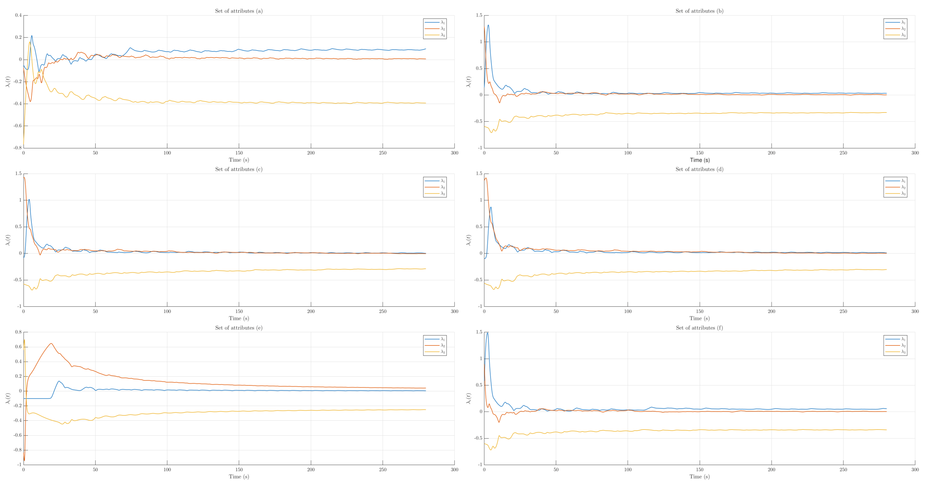
The first set, corresponding to a i = 6 , presents a positive maximum exponent ( λ i , max = 0.026334 ), confirming the presence of chaos and the exponential divergence of nearby trajectories. This behavior remained consistent across multiple code executions, indicating an intrinsically unstable dynamic associated with low saving rates.
In contrast, the sets with a i = 7.07, 7.15, 7.20, and 8.30 exhibit negative exponents, reflecting stability and the absence of chaotic behavior.
For the last case, where a i = 7.03 , the maximum exponent is close to zero ( λ i , max = 0.000881 ), indicating a dynamic behavior at the edge of chaos, where small variations in the parameter can induce rapid transitions between stable and unstable regimes.
Lyapunov spectrum, shown in Figure 5, allows the identification of well-defined stability and chaos regions, as the values of λ i , max precisely delimit the intervals of the parameter a i in which the system transitions from one regime to another. In particular, positive values correspond to chaotic regions with unpredictable behavior, values close to zero mark quasi-periodic transition zones, and negative values indicate stable and periodic state.

4.5. Results of Impulsive Pinning Control

A strategic subset of nodes is selected using a genetic algorithm to apply the impulsive pinning control, prioritizing those with higher connectivity and topological influence. The genetic algorithm is implemented with a population of 50 individuals, evolving over 150 generations. Selection followed a roulette-wheel criterion, with crossover and mutation probabilities of 0.8 and 0.05, respectively. The optimization stopped when the global synchronization error J < 10 3 or when convergence is reached over 30 consecutive generations. Once the control is applied, a rapid reduction in the oscillations of the state variables and a global synchronization of the system toward the equilibrium point ( x , y , z ) = ( 0 , 10 , 0 ) are considered.
The results show that the impulsive pinning control is capable of stabilizing the system by applying discrete interventions over a small fraction of nodes. The mean square error between the controlled nodes and the reference state decreased by more than 90% during the first impulses, confirming the energy efficiency of the method and the feasibility of achieving global control with minimal effort.
From an economic perspective, these results suggest that focused policies targeting key actors within the financial system can generate large-scale stabilizing effects, preventing the propagation of crises through limited but strategically applied interventions.

4.6. Economic Interpretation

The chaotic dynamics observed in the results can be interpreted as a structural financial crisis arising from low saving levels or insufficient investment. The application of impulsive pinning control represents, in economic terms, the implementation of periodic regulatory measures or liquidity injections aimed at stabilizing the most unstable markets.
The synchronization observed in the network symbolizes the global coordination of financial policies that lead to the restoration of systemic equilibrium. The results confirm that financial crises can be mitigated through direct, discrete interventions targeting a reduced number of critical agents.
This perspective allows a more realistic modeling of the interactions among interdependent economies and the recovery of stability under polycrisis conditions, providing an analytical framework for the design of control strategies and the strengthening of economic resilience.

5. Discussion

Numerical results show that even when only two nodes in the financial network operate in a chaotic regime (nodes 1 and 2), instability can propagate through the coupling structure and affect the behavior of nodes that are initially stable. This observation confirms the hypothesis that localized crises can escalate into systemic disruption when interconnections play an active role in transmission, consistent with network-based perspectives of systemic risk [3,5].
It should be noted that these results are obtained entirely under controlled synthetic conditions [14]. The use of synthetic data allows isolating the intrinsic nonlinear dynamics of the system and evaluating the effectiveness of the impulsive pinning control without the confounding influence of noise, regime shifts, or structural breaks commonly found in empirical financial time series. Future work will extend the analysis to real financial data in order to assess the practical relevance and robustness of the proposed control strategy under real-world conditions.
Before intervention, the maximum Lyapunov exponent remains positive in several parameters, evidencing sensitivity to initial conditions and unpredictable oscillatory patterns in macroeconomic variables. Such characteristics align with emerging financial crises, where volatility rapidly amplifies due to speculation dynamics, credit limitations, and liquidity constraints.
After introducing impulsive pinning control to optimal subset of nodes selected by a genetic algorithm, a clear transition occurs in the dynamic regime: oscillations attenuate, and state trajectories converge toward equilibrium. The maximum Lyapunov exponent becomes negative, confirming chaos suppression and global stabilization of financial network. These findings reinforce previous studies showing that partial control based on network topology can efficiently synchronize nonlinear systems [17].
Importantly, the proposed stabilization strategy requires control action on only a small fraction of nodes, which significantly reduces the control effort compared to centralized or full-network interventions. This behavior resembles targeted regulatory or monetary interventions in real financial systems (e.g., liquidity injections or focused supervisory actions), where supporting systemically important nodes prevents widespread failure propagation.
These results directly support the main objective of this work, which is to show that full stabilization of a financial network in crisis can be achieved through partial impulsive pinning control acting only on a limited subset of critical nodes.
Findings suggest that chaotic behavior represents not only mathematical instability but also a metaphor for a highly vulnerable regime within global finance. Controlling this instability at a structural level may improve systemic resilience under conditions of polycrisis, where multiple disruptions interact and amplify fragility [1]. This strengthens the conceptual argument that financial markets should not be analyzed as isolated entities but rather as co-evolving subsystems embedded within global interdependencies.
We acknowledge that this study does not incorporate real weighted exposure data, such as bilateral lending, interbank liabilities, or institution-level balance-sheet linkages. Weighted financial networks and size-based pinning strategies—particularly approaches that prioritize “pinning largest institutions first”—offer essential directions for future extensions, as they capture heterogeneous exposure magnitudes and the structural influence of systemically essential institutions more accurately. Although integrating real weighted data lies beyond the scope of this manuscript, we explicitly recognize this limitation and highlight these modeling approaches as primary avenues for future research.
Future research directions include moving beyond the synthetic setting considered in this study by incorporating real-world financial network data, stochastic variations of parameters, and adaptive control strategies capable of responding to rapidly changing market conditions. Such extensions will make it possible to evaluate the practical relevance and robustness of the proposed impulsive pinning control under real-world conditions and help translate these theoretical findings into practical tools for early warning and targeted stabilization of systemic financial risk.

6. Conclusions

Viewing financial instability through a complex network perspective provides new insight into how crises emerge and propagate across interconnected markets. Representing each economy as a nonlinear dynamic system with the potential for chaotic behavior allowed us to show that systemic disruptions can arise even when instability is initially confined to only a few nodes.
A key outcome of this study is that full stabilization of the financial network can be achieved through impulsive pinning control applied only to a strategically selected subset of nodes. This challenges traditional assumptions requiring centralized or full-network interventions to mitigate crisis conditions and instead shows that effective control may be delivered through minimal, well-targeted actions.
These results strengthen the argument that global finance should be analyzed as a co-evolving network in which local failures may amplify and spread through structural dependencies. Proposed stabilization mechanism supports the design of selective and cost-efficient systemic risk policies capable of containing volatility before it cascades into global collapse.
Future work will integrate empirical financial connectivity data, examine robustness under parameter uncertainty, and develop adaptive control strategies capable of responding to rapidly changing market conditions. These extensions will help translate the theoretical findings into practical tools for early warning and selective stabilization within real financial environments.

Author Contributions

Investigation, H.G.V., P.M.G., A.I. and A.Y.A.; Methodology, A.Y.A., H.G.V. and J.G.; Software, A.Y.A. and H.G.V.; Supervision, A.Y.A. and J.G.A.; Visualization, H.G.V.; Writing—original draft, H.G.V., P.M.G. and A.I.; Writing—review and editing, A.Y.A., E.M.-P., J.G.A., P.M.G., H.G.V. and A.I.; Development of Methodology, A.Y.A. and H.G.V. All authors have read and agreed to the published version of the manuscript.

Funding

The authors gratefully acknowledge the Centro Universitario de Ciencias Exactas e Ingenierías (CUCEI) of the Universidad de Guadalajara for covering the Article Processing Charge (APC).

Data Availability Statement

The original contributions presented in this study are included in the article. Further inquiries can be directed to the corresponding authors.

Acknowledgments

The authors thank the Universidad de Guadalajara for supporting the development of this research. The authors used generative artificial intelligence (AI) tools to support language editing and writing improvements in this manuscript. The AI tool is used solely for improving grammar, phrasing, and clarity in English and did not contribute to the study’s conceptualization, data analysis, or interpretation. The authors reviewed and edited the output and take full responsibility for the content, accuracy, and integrity of the publication.

Conflicts of Interest

The authors declare no conflicts of interest.

References

  1. Forum, W.E. The Global Risks Report 2025, 20th ed.; World Economic Forum: Geneva, Switzerland, 2025. [Google Scholar]
  2. Ergüzel, O. Chaos Theory and Financial Markets: A Systematic Review of Crisis and Bubbles. Chaos Theory Appl. 2025, 7, 70–77. [Google Scholar] [CrossRef]
  3. Huang, C.; Miao, H.; Yang, X.; Cao, J.; Yang, H. Cascading failure, financial network and systemic risk. N. Am. J. Econ. Financ. 2025, 80, 102505. [Google Scholar] [CrossRef]
  4. Gao, Q.; Ma, J. Chaos and Hopf Bifurcation of a Finance System. Nonlinear Dyn. 2009, 58, 209–216. [Google Scholar] [CrossRef]
  5. Battiston, S.; Farmer, J.; Flache, A.; Garlaschelli, D.; Haldane, A.; Heesterbeek, H.; Scheffer, M. Complexity Theory and Financial Regulation. Science 2016, 351, 818–819. [Google Scholar] [CrossRef] [PubMed]
  6. Chen, G. Pinning Control of Complex Dynamical Networks. IEEE Trans. Consum. Electron. 2022, 68, 336–343. [Google Scholar] [CrossRef]
  7. Wang, X.; Chen, G. Pinning Control of Complex Networked Systems; Springer: Berlin/Heidelberg, Germany, 2013. [Google Scholar] [CrossRef]
  8. Della Rossa, F.; Liuzza, D.; Lo Iudice, F.; De Lellis, P. Nonlinear Pinning Control of Stochastic Network Systems. Automatica 2023, 149, 110826. [Google Scholar] [CrossRef]
  9. Li, K.; Yang, L.; Guan, C.; Leng, S. Reinforcement learning-based pinning control for synchronization suppression in complex networks. Heliyon 2024, 10, e34065. [Google Scholar] [CrossRef] [PubMed]
  10. Orouskhani, Y.; Jalili, M.; Yu, X. Optimizing Dynamical Network Structure for Pinning Control. Sci. Rep. 2016, 6, 24252. [Google Scholar] [CrossRef] [PubMed]
  11. Wolf, A.; Swift, J.; Swinney, H.; Vastano, J. Determining Lyapunov Exponents from a Time Series. Phys. D Nonlinear Phenom. 1985, 16, 285–317. [Google Scholar] [CrossRef]
  12. Cheng, Z.; Xin, Y.; Cao, J.; Li, P.; Liu, J. Selecting pinning nodes to control complex networked systems. Sci. China Technol. Sci. 2018, 61, 1537–1545. [Google Scholar] [CrossRef]
  13. Wang, L.; Guo, Y.; Wang, Y.; Fan, H.; Wang, X. Pinning Control of Cluster Synchronization in Regular Networks. Phys. Rev. Res. 2020, 2, 023084. [Google Scholar] [CrossRef]
  14. Tait, J. Synthetic Data in Investment Management; Technical report; CFA Institute: Singapore, 2025. [Google Scholar]
  15. Bharali, A.; Doley, A. On Small-World and Scale-Free Properties of Complex Network. Int. J. Math. Stat. Invent. (IJMSI) 2017, 5, 11–16. [Google Scholar]
  16. Sun, Y.; Li, L.; Ho, D.W.C. Synchronization Control of Complex Dynamical Networks: Invariant Pinning Impulsive Controller With Asynchronous Actuation. IEEE Trans. Netw. Sci. Eng. 2022, 9, 4255–4265. [Google Scholar] [CrossRef]
  17. Sun, W.; Lü, J.; Chen, S.; Yu, X. Pinning impulsive control algorithms for complex network. Chaos Interdiscip. J. Nonlinear Sci. 2014, 24, 013141. [Google Scholar] [CrossRef] [PubMed]
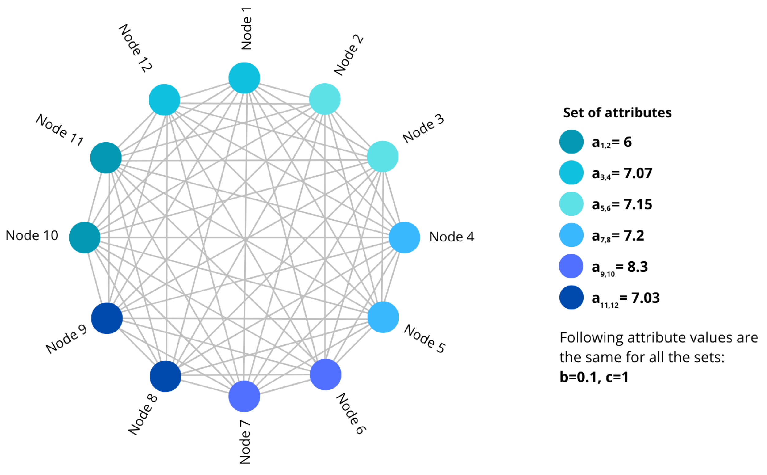
Figure 1. Network topology and parameter mapping.
Mathematics 13 03922 g001
Figure 2. Typical dynamical behavior of system: (a) a 1 , 2 = 6, (b) a 3 , 4 = 7.07, (c) a 5 , 6 = 7.15, (d) a 7 , 8 = 7.2, (e) a 9 , 10 = 8.3, (f) a 11 , 12 = 7.03.
Mathematics 13 03922 g002
Figure 3. Node behavior.
Mathematics 13 03922 g003
Figure 4. Complex Network State.
Mathematics 13 03922 g004
Figure 5. Lyapunov exponent’s spectrum of the system. (a) a i = 6 , (b) a i = 7.07 , (c) a i = 7.15 , (d) a i = 7.2 , (e) a i = 8.3 , (f) a i = 7.03 .
Mathematics 13 03922 g005
Table 1. Dynamic regimes as a function of saving parameter a i .
Range of a i Dynamic RegimeFinancial Interpretation
0 < a i 6.42 and 6.61 < a i 7.02 ChaoticDeep crisis and financial instability
6.41 < a i 6.60 and 7.03 < a i 7.09 2D TorusUnstable adjustments preceding chaos
7.10 < a i 8.94 PeriodicRegular economic cycles
8.95 < a i 10 StableEconomy in equilibrium
Table 2. Model nomenclature summarizing variables and parameters of the nonlinear financial network.
SymbolDescription
x i Interest rate associated with financial node i
y i Investment demand of node i
z i Price index linked to node i
x ˙ i , y ˙ i , z ˙ i Time derivatives of macroeconomic variables
a i Saving parameter or economic sensitivity of node i
bDamping coefficient in investment demand
cRigidity coefficient of price level
NTotal number of financial nodes in the network
X i = [ x i , y i , z i ] T State vector of node i
X r = [ x r , y r , z r ] T Reference or desired equilibrium vector
A = [ a i j ] Adjacency matrix describing connectivity among nodes
ε Coupling or financial correlation intensity among nodes
σ Global coupling gain of the system
g i Control gain applied to node i (in pinning control scheme)
TSampling period or interval between control impulses
P , Q Positive-definite matrices used in LMI conditions for impulsive stability
λ max Maximum Lyapunov exponent used to assess system stability
JGlobal mean-squared synchronization error (objective function in genetic algorithm)
Table 3. Parameter assignment of a i in a 12-node financial network.
Node(s) a i Dynamic RegimeEconomic Interpretation
1–26.00ChaoticEconomies in crisis
3–47.07Transition (near-chaotic)Early recovery phase
5–67.15Quasi-periodicVulnerable economies
7–87.20Periodic/StableHealthy economies
9–108.30Stable/RobustWell-regulated economies
11–127.03Chaotic/UnstableEconomies entering crisis
Table 4. Scalability analysis for networks of N = 100 nodes under different connectivity levels using the Lorenz–financial model with impulsive pinning control.
Connectivity (%)J (Mean-Squared Error) λ max E c (Control Energy)
25%0.03079.26497117
50%0.03009.32498248
75%0.03029.33095674
100%0.026810.53495461
Disclaimer/Publisher’s Note: The statements, opinions and data contained in all publications are solely those of the individual author(s) and contributor(s) and not of MDPI and/or the editor(s). MDPI and/or the editor(s) disclaim responsibility for any injury to people or property resulting from any ideas, methods, instructions or products referred to in the content.