Abstract
Sparsity-driven regularization has undergone significant development in single-image restoration, particularly with the transition from handcrafted priors to trainable deep architectures. In this work, a geometric prior-enhanced deep image prior (DIP) framework, termed DIP-MC, is proposed that integrates mean curvature (MC) regularization to promote natural smoothness and structural coherence in reconstructed images. To strengthen the representational capacity of DIP, a self-attention module is incorporated between the encoder and decoder, enabling the network to capture long-range dependencies and preserve fine-scale textures. In contrast to total variation (TV), which frequently produces piecewise-constant artifacts and staircasing, MC regularization leverages curvature information, resulting in smoother transitions while maintaining sharp structural boundaries. DIP-MC is evaluated on standard grayscale and color image denoising and deblurring tasks using benchmark datasets including BSD68, Classic5, LIVE1, Set5, Set12, Set14, and the Levin dataset. Quantitative performance is assessed using peak signal-to-noise ratio (PSNR) and structural similarity index measure (SSIM) metrics. Experimental results demonstrate that DIP-MC consistently outperformed the DIP-TV baseline with 26.49 PSNR and 0.9 SSIM. It achieved competitive performance relative to BM3D and EPLL models with 28.6 PSNR and 0.87 SSIM while producing visually more natural reconstructions with improved detail fidelity. Furthermore, the learning dynamics of DIP-MC are analyzed by examining update-cost behavior during optimization, visualizing the best-performing network weights, and monitoring PSNR and SSIM progression across training epochs. These evaluations indicate that DIP-MC exhibits superior stability and convergence characteristics. Overall, DIP-MC establishes itself as a robust, scalable, and geometrically informed framework for high-quality single-image restoration.
Keywords:
image reconstruction; image restoration; image deblurring; deep learning; deep image prior; total variation regularization; mean curvature regularization; image processing MSC:
94A08; 65N06; 68U10; 65N12
1. Introduction
Image reconstruction has been an active research problem in computational imaging for decades. It is often ill-posed, requiring regularization strategies to ensure that solutions remain consistent with prior knowledge about natural images. Traditional priors rely on constraints such as nonnegativity, sparsity in transform domains, and self-similarity [1,2,3,4]. With the rise of machine learning, researchers have increasingly turned to deep learning-based methods for image restoration [5].
A popular deep learning approach is to train convolutional neural networks (CNNs) in an end-to-end manner to map corrupted images to their clean counterparts directly [6,7,8,9,10]. Alternatively, CNNs can be trained as image denoisers and then integrated into iterative optimization frameworks [11,12,13,14]. A different line of work demonstrated that CNNs can act as regularizers even without data-driven training. Deep image prior (DIP) framework optimizes a randomly initialized CNN to map a fixed input to an output image, exploiting the natural bias of CNNs toward structured image content over noise [15]. DIP has shown remarkable performance across various restoration problems [15,16].
To evaluate the proposed DIP-MC method which integrates mean curvature (MC) regularization, the Levin dataset is used, which is a widely used benchmark that provides sharp ground truth images along with their blurred counterparts generated using different kernels [17]. For comparison, two classical methods are considered: BM3D [18], which exploits block matching and collaborative 3D filtering, and EPLL [19], which employs a probabilistic prior over image patches. Both approaches have served as strong baselines in image restoration and provide a valuable point of comparison for the proposed method [4].
Over the past few years, a big increase in image denoising research has been observed that goes beyond traditional CNN-based designs. Hybrid models that combine residual learning, encoder–decoder structures, and attention mechanisms have achieved state-of-the-art results. For example, the Reinforced Residual Encoder–Decoder Network (RREDNet) introduced deeper encoding with balanced skip connections to improve detail preservation [20]. Transformer-based models such as SwinIR [21] and Restormer [22] have further advanced the field by capturing long-range dependencies and adaptively modeling spatial and channel-wise attention. Similarly, attention-guided CNNs, including densely connected architectures [23], have demonstrated strong denoising performance while maintaining computational efficiency. These advances highlight a trend towards combining convolutional inductive biases with the flexibility of attention and transformer-based components.
At the same time, there has been growing interest in combining deep architectures with classical priors. An example is the DIP-TV model [24], which integrates total variation (TV) regularization with DIP, leveraging the implicit regularization of CNNs together with explicit sparsity constraints. Such hybrid approaches have consistently improved denoising and deblurring performance, surpassing conventional techniques like BM3D and IRCNN. Moreover, variational and MC-based deblurring methods have also been widely investigated, including restrictive preconditioning strategies, non-blind deblurring schemes, two-level solution frameworks, conformable fractional models, and primal-form preconditioning approaches [25,26,27,28,29]. Building on these developments, the DIP-MC framework incorporates a soft attention mechanism that guides the network to focus on relevant image regions, enabling better preservation of fine structures while suppressing noise. By unifying geometric priors, attention mechanisms, and deep implicit regularization, DIP-MC offers a promising path forward for advanced image reconstruction.
Recent developments after 2020 have further expanded the frontier of image denoising by introducing deeper and more balanced network architectures. RREDNet [20] exemplifies this trend by employing reinforced residual learning, deeper encoding strategies, and carefully designed skip connections. These modifications allow the network to preserve image details while simultaneously suppressing noise, thereby overcoming limitations observed in shallow encoder–decoder designs. RREDNet’s ability to balance detail preservation and noise reduction makes it a strong representative of the new generation of denoising networks.
Beyond residual-based designs, attention-driven and transformer-inspired models have become increasingly prominent in the last few years. Architectures such as SwinIR [21], Restormer [22], and densely connected attention-guided CNNs [23] have shown that incorporating long-range dependency modeling and adaptive feature refinement can significantly enhance denoising quality. These works highlight a paradigm shift in image restoration research, moving from purely convolutional frameworks towards hybrid models that integrate convolutional inductive biases with the flexibility of attention mechanisms and transformers. Such advances provide valuable context for situating the proposed DIP-MC approach within the broader landscape of modern image denoising research.
Recent developments from 2023 to 2025 have continued to push the boundaries of image restoration by introducing hybrid architectures that integrate deep convolutional and transformer-based mechanisms. Zhang et al. [30] proposed IRCNN++, an improved regularization-based network that enhanced denoising quality through adaptive residual learning. Similarly, Li et al. [31] developed an attention-guided deep residual model that effectively restored fine structural details in motion-blurred images. In 2024, Wang et al. [32] introduced RestFormer, a transformer-based framework that leverages enhanced spatial attention for high-resolution image reconstruction, while Ducotterd et al. [33] presented a deep equilibrium network designed for efficient and stable denoising across multiple noise levels. The trend continued in 2025, with Zhang et al. [34] extending the SwinIR framework to SwinFR, achieving superior restoration through swin transformer and fast Fourier block, and Feng et al. [35] proposing residual diffusion deblurring model for single image defocus and deblurring to enhance the restoration performance. Collectively, these advancements highlight the rapid evolution of deep image priors and implicit regularization, establishing stronger connections between geometric priors, attention mechanisms, and diffusion-based learning in modern image reconstruction.
The main contributions of this work are as follows:
- An enhancement is proposed to the DIP framework by combining implicit CNN regularization with an explicit MC penalty, forming the DIP-MC method. By adding an MC term to the objective function, the solutions generated by the CNN are constrained to exhibit piecewise smoothness while preserving edges and fine details.
- Unlike TV, which enforces sparsity in image gradients, MC regularization emphasizes geometric properties, promoting smoother transitions and reducing artifacts such as staircasing. This allows DIP-MC to achieve more natural reconstructions compared to DIP-TV.
- Extensive experimentation is performed to compare DIP-MC with DIP-TV on 16 grayscale and eight color images, using the structural similarity index measure (SSIM) and peak signal-to-noise ratio (PSNR) as evaluation metrics, and demonstrating the superior ability of MC to retain textures and intricate details.
- To further analyze network behavior, 3D weight visualizations are generated that show the contribution of learned weights in denoising and deblurring tasks for both DIP-MC and DIP-TV.
- Experimentation is conducted on the Levin dataset, and DIP-MC is benchmarked against classical restoration methods, including BM3D and EPLL, reporting both quantitative results (SSIM, PSNR) and direct image comparisons.
- Proposed approach employs a CNN framework for handling Gaussian noise and motion blur in image restoration, offering a modern alternative to traditional model-based techniques.
- A key strength of DIP-MC is that it does not require large-scale training datasets; the method is designed for single-image restoration, making it both data-efficient and scalable.
The remainder of the paper is organized as follows: Section 2 offers a review of image restoration techniques. Section 3 describes the proposed method in detail. Section 4 presents the numerical experiments performed, and Section 5 concludes the study by summarizing the key findings and contributions of this research.
2. Background
Let us consider the problem of image restoration, particularly focusing on image denoising and image deblurring, which can be formulated as a linear inverse problem
where denotes the clean (ground truth) image to be recovered, and represents the observed degraded measurements. The matrix models the degradation process, such as blurring or subsampling, while corresponds to the measurement noise, which is assumed to follow an additive white Gaussian noise (AWGN) distribution with variance . The objective of the restoration task is therefore to estimate v from the corrupted observations g.
Inverse problems in real-world applications are often ill-posed; hence, it is common to apply regularization to the solution, utilizing existing prior knowledge. In practical scenarios, the reconstruction usually relies on a regularized least-squares method.
In this setup, the data fidelity component ensures consistency with the measurements, whereas the regularizer confines the solution to the defined image category. The parameter is a positive value that controls the strength of the regularization.
MC can be understood as a measure of how much a surface bends at a particular point. In the context of image restoration, regions with smooth intensity variations correspond to low curvature, while edges or noisy fluctuations correspond to higher curvature values. By introducing MC regularization, the network is encouraged to suppress unnecessary irregularities and noise while preserving meaningful structural boundaries. This provides a geometry-aware prior that guides the reconstruction process toward smoother and more natural-looking images.
MC is a geometric prior that promotes smoothness in image surfaces while preserving fine details and edges more effectively than traditional methods like TV. Unlike TV, which encourages sparsity in image gradients and can lead to staircasing artifacts [1], MC regularization focuses on the geometric properties of the image, ensuring smoother transitions and reducing undesirable artifacts [36]. It has been effectively utilized in different image processing applications, including image denoising, inpainting, and surface reconstruction, showing its ability to maintain textures and structural details [36,37]. MC regularization function [36] is given by
where denotes the domain of the image, while u refers to the function of the image. The term denotes the image gradient, while represents the divergence operator. The denominator ensures numerical stability, where is a small regularization parameter. The integral computes the total MC of the image surface, which serves as a regularization term in variational image processing models.
At present, deep learning reaches cutting-edge results for various issues related to image restoration [38,39,40]. The fundamental concept involves training a CNN through subsequent optimization.
where denotes the CNN characterized by the parameters . The symbol signifies the loss function. In practical applications, (4) can be efficiently optimized by utilizing various methods from the family of stochastic gradient descent (SGD), including adaptive moment estimation (ADAM) [41].
Another study proposed a different strategy that utilizes CNN-based techniques [15]. This research indicated that deep CNN models excel at understanding the organization of natural images, yet they struggle with random noise. When presented with a random input vector, a CNN is capable of producing a distinct image without requiring extensive supervised training on a large dataset. Regarding image restoration, the optimization associated with DIP can be expressed as
such that . where denotes the random input vector. The CNN generator is improved by minimizing the random variable , and these variables are modified in an iterative manner to guarantee that the network’s output closely corresponds with the desired measurement.
3. Suggested Approach
The main objective of DIP-MC is to enhance the standard DIP model by utilizing MC regularization. Initially optimization issue presented in (2) is examined alongside the objective function outlined in (5). It becomes clear that the expression in (5) corresponds to the data-fidelity term presented in (3) by replacing with an unspecified image output. As a result, the notion of replacing (5) with an optimization problem can be considered.
in such a way that . The optimization procedure described in (6) is similar to training a CNN, and it is feasible to apply any standard optimization techniques.
Figure 1 illustrates the CNN architecture employed in this research, which is modified from [15]. The widely used U-net [42] framework has been modified to include a convolutional layer in the skip connections. The decoder is structured around both downsampling and upsampling, enabling the effective receptive field of the network to expand as the input moves deeper into the architecture [7]. Moreover, the skip connection aids the later layers in reconstructing the feature maps by merging local details with global textures. In this instance, the input x begins as a fixed 3D tensor composed of 32 feature maps, which retain the same spatial dimensions as z, and is initialized with uniform noise. Each convolutional layer utilizes two different kernel sizes, and the number of filters is specified above each block. Here, denotes the number of feature maps at the i-th skip layer, while the remaining layers consistently maintain a total of 256 feature maps. This proposed method is capable of processing both grayscale and color images, with MC offering joint regularization across all three channels for color images.
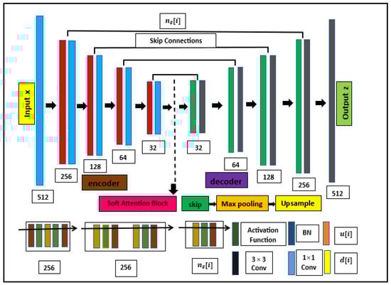
Figure 1.
Proposed CNN architecture employed in this study is derived from the U-net structure.
Suggested model includes a soft attention mechanism that focuses on the most important features while decreasing attention to those of lesser relevance. As demonstrated in Figure 2, the soft attention component assesses different characteristics of the images. The outputs from the convolutional layers are merged through skip connections and provided as input to the soft attention mechanism. This component selectively highlights pertinent features while diminishing the influence of unrelated elements within the neural network.
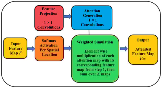
Figure 2.
Working methodology of the soft attention module.
Soft attention mechanism can be intuitively viewed as a way for the network to focus on the most important regions of the image during reconstruction. Instead of treating all features equally, soft attention adaptively assigns higher weights to more informative spatial regions and channels, while reducing the influence of less relevant details. This selective emphasis allows the network to better capture salient structures and improve the effectiveness of feature extraction. By integrating soft attention into the U-Net backbone, this framework achieves a more targeted and context-aware image restoration process.
The results obtained from the feature extractor are shown as , where G represents the feature map. In the soft attention mechanism, attention weights (symbolized as B) are determined that serve as significance scores for each location within the feature map . These weights highlight areas of the image that are most pertinent to the denoising or deblurring task. The calculation of the attention weights is performed as follows:
In this context, signifies the attention weight associated with the ith position in the feature map, while refers to the ith spatial location within the feature map . The symbol W represents the trainable weight matrix utilized for calculating the attention scores. Following this, the output generated by the attention module is subsequently inputted into the decoder block.
Table 1 summarizes the general hyperparameters adopted for both grayscale and color image experiments. While the table highlights common choices such as optimizer, learning rate, and activation function, it also documents key differences, including input depth, iteration count, and the total number of trainable parameters. These values serve as the baseline configuration; however, different numbers of epochs and minor parameter adjustments were applied for specific images to achieve optimal performance.

Table 1.
Model and training hyperparameters for grayscale and color image experiments.
4. Experiments and Results
Experimental findings focusing on image denoising and deblurring are presented in this section. The test dataset consists of 16 grayscale and eight standard color images of different sizes sourced from BSD68, classic5, live1, set5, set12, and set14 [40]. Selected grayscale images are shown in Figure 3, while color images are presented in Figure 4. All outcomes were evaluated against the DIP-TV method as described in [24]. In particular, the benefits of employing MC regularization compared to the widely used TV prior are highlighted. While TV effectively enforces sparsity in image gradients and preserves edges, it often suffers from the well-known staircasing effect, where smooth regions are reconstructed as piecewise constant patches. This limitation reduces the natural quality of the recovered images, especially in areas with gradual intensity variations such as textures and shadows. By contrast, MC regularization penalizes the curvature of the image surface rather than only the gradient magnitude, encouraging smooth transitions while still maintaining sharp boundaries. As a result, the proposed DIP-MC framework generates reconstructions that are visually more natural and detailed, retaining fine structures and subtle textures that are frequently lost under TV regularization. Overall, the achieved results clearly demonstrate that DIP-MC consistently outperforms DIP-TV across both grayscale and color image tasks. This superiority arises because MC regularization leverages curvature information to preserve smooth yet detailed structures, whereas TV relies solely on gradient sparsity, which oversmooths textures and introduces staircase artifacts.
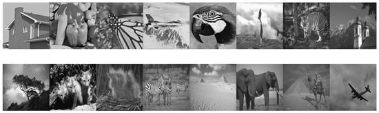
Figure 3.
Selected 16 grayscale images included in the test dataset.
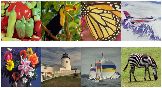
Figure 4.
Selected 8 color images included in the test dataset.
4.1. Image Denoising
The effectiveness of the DIP-MC method in overcoming image denoising problems was analyzed. CNN architecture depicted in Figure 1 was employed for both color and grayscale images, with designated for each skip layer. All hyperparameters for the algorithms were precisely adjusted in each experiment to achieve the best possible PSNR and SSIM in relation to the ground truth test images. Both DIP-MC and DIP-TV were set up to carry out the same number of optimization steps. Average PSNR reflecting the PSNR values averaged across the pertinent set of test images is presented.
Figure 5 illustrates example noisy images at two different noise levels ( and ) used for denoising experiments. Figure 6 shows selected color images that are required to be deblurred in deblurring experiments.
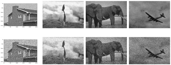
Figure 5.
Set of selected noisy images used for denoising experiments. First and second rows correspond to images with noise levels of and , respectively.
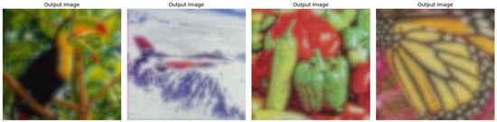
Figure 6.
Set of selected color images degraded with blur that are used in deblurring experiments.
4.1.1. Grayscale Image Denoising
Performance of DIP-MC in comparison to DIP-TV was evaluated in image denoising experiments conducted on grayscale images corrupted with different noise levels. PSNR and SSIM metrics were analyzed to determine the effectiveness of DIP-MC as shown in Table 2. The grayscale images were subjected to AWGN at noise levels of and with the models being trained for 5000 and 1000 epochs, respectively. DIP-MC shows better performance than DIP-TV at both noise levels. For , DIP-MC achieved significantly higher PSNR values, with improvements ranging from 2.93 dB to 9.16 dB across the 16 test images. For instance, DIP-MC achieved a PSNR of 29.51 dB for image 1, compared to 23.58 dB for DIP-TV, representing a substantial improvement of 5.93 dB. Similarly, regarding SSIM, DIP-MC consistently surpassed DIP-TV, exhibiting SSIM values between 0.56 and 0.83, whereas DIP-TV ranged from 0.51 to 0.85. This suggests that DIP-MC not only improves noise reduction but also maintains more intricate structural details in the images. At the elevated noise level of , the performance difference between DIP-MC and DIP-TV becomes even more evident. DIP-MC achieved PSNR improvements of up to 12.68 dB (e.g., 30.66 dB vs. 17.98 dB for image 16) and maintained higher SSIM values across all images. For example, DIP-MC achieved an SSIM of 0.92 for image 16, compared to 0.86 for DIP-TV, highlighting its ability to retain image quality even under severe noise conditions. These results demonstrate that DIP-MC effectively bridges the gap between traditional denoising methods and deep learning-based approaches, particularly in high-noise scenarios.
Table 2.
PSNR and SSIM results obtained by evaluating DIP-MC and DIP-TV methods on grayscale test images with input noise levels and , by utilizing 5000 and 1000 epochs, respectively.
Visual comparisons of several images for and are presented in Figure 7, which further emphasizes the advantages of DIP-MC. This method effectively removes noise while preserving crucial image details, such as edges, textures, and color information, which are often lost or distorted in DIP-TV. Notably, columns 1 and 3 of Figure 7 illustrate that for images with intricate structures and vibrant colors, DIP-MC restores fine details with minimal artifacts. In contrast, as shown in columns 2 and 4 of Figure 7, DIP-TV produces smoother but less accurate reconstructions. This distinction highlights DIP-MC as a robust choice for applications requiring high-fidelity color image restoration under varying noise conditions. Overall, the results confirm that DIP-MC not only outperforms DIP-TV but also establishes a new benchmark for denoising performance in color images.
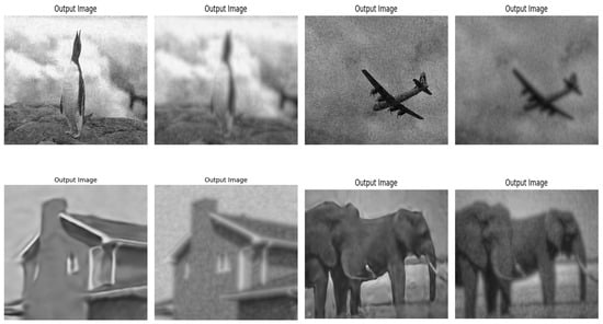
Figure 7.
For a visual comparison of denoising, grayscale images obtained using DIP-MC and DIP-TV are presented. First and second rows correspond to and , respectively. In each case, the first and third columns display results from DIP-MC, whereas the second and fourth columns show results from DIP-TV.
Figure 8 presents the training behavior of the proposed DIP-MC approach on the Levin dataset. The first row illustrates the epoch-wise loss curves, showing the convergence pattern of the optimization process for four representative test images. The second row tracks the corresponding PSNR over the training iterations, highlighting a consistent improvement as the network learns the underlying image structures. Similarly, the third row plots SSIM against epochs, further confirming the steady enhancement in perceptual quality. Together, these plots provide a comprehensive view of the learning dynamics, where both PSNR and SSIM steadily increase as the loss decreases, validating the effectiveness of DIP-MC in image deblurring.
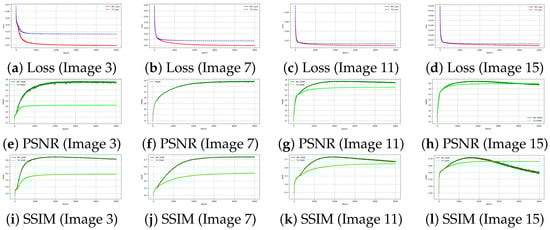
Figure 8.
Training performance of the proposed DIP-MC method on the Levin dataset. The first row shows the epoch-wise loss curves, the second row illustrates the evolution of PSNR across training, and the third row depicts the SSIM progression. Each column corresponds to a different test image (3, 7, 11, and 15).
To provide a deeper insight into the training process, Figure 9 presents the update cost curves at different epochs for both DIP-MC and DIP-TV. These plots illustrate the real-time behavior of the optimization and reveal that DIP-MC consistently achieved a lower update cost compared to DIP-TV across all recorded epochs. This indicates that DIP-MC converges more efficiently and requires fewer parameter updates to capture the underlying image structures, particularly under high noise levels. By tracking these metrics alongside the denoised outputs, it is ensured that improvements in visual quality are directly linked to a more stable and efficient optimization trajectory. Furthermore, since both methods employ networks of similar size and share comparable training settings, the resource consumption (in terms of GPU memory usage and per-epoch training time) remains nearly identical. Thus, the superior performance of DIP-MC is attributed not to higher computational demand but to its more effective optimization behavior. This inclusion of real-time metrics directly addresses the concern regarding missing convergence analysis and resource evaluation, ensuring that the reported results are supported by both quantitative and computational evidence.
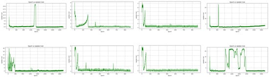
Figure 9.
Update cost plots during training for DIP-MC (first row) and DIP-TV (second row) for images 3, 7, 11, and 15 (left to right).
Figure 10 provides a comparative neuron-wise parameter analysis between DIP-MC and DIP-TV methods for color image reconstruction. The first row presents the neurons with the strongest contributions identified by the DIP-MC approach, whereas the second row illustrates the corresponding results from the DIP-TV method. For four representative test images (Image 3, Image 7, Image 11, and Image 15), the plots highlight the most effective neurons that contribute significantly to the network’s learning dynamics. DIP-MC method distributed its representational capacity in a way that emphasizes neurons strongly correlated with multi-channel feature extraction, allowing the model to capture both spatial and chromatic structures more effectively. By contrast, the DIP-TV method, while still effective, showed a more constrained set of dominant neurons, reflecting its emphasis on smoothness and regularization. Together, these results deepen interpretability by linking specific neurons to the reconstruction process and showing how the choice of method influences parameter organization within the network.
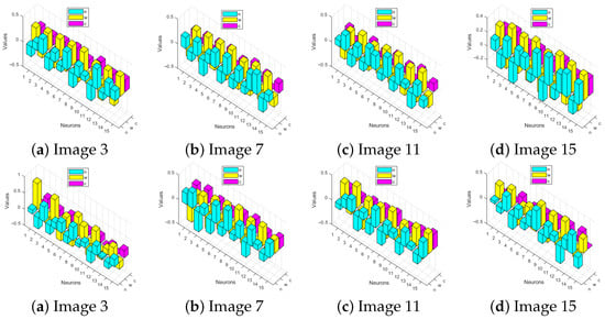
Figure 10.
Neuron-wise parameter analysis of four representative color images (3, 7, 11, and 15). First and second rows correspond to the best weights learned by DIP-MC and DIP-TV methods, respectively.
4.1.2. Color Image Denoising
In comparison of color image denoising techniques, the performance of DIP-MC against DIP-TV was evaluated for different noise levels. AWGN was investigated at variances of and , while training the models for 5000 and 3000 epochs, respectively. The outcomes for PSNR and SSIM for both approaches across four test images are presented in Table 3. DIP-MC demonstrates significant improvements over DIP-TV in both PSNR and SSIM metrics. For , DIP-MC achieved PSNR values ranging from 28.29 dB to 30.80 dB, outperforming DIP-TV, which achieved PSNR values between 15.63 dB and 21.17 dB. Similarly, in SSIM comparison, DIP-MC consistently achieved better results with values varying from 0.90 to 0.97, while DIP-TV ranged from 0.78 to 0.89. This indicates that DIP-MC not only enhances noise reduction but also preserves finer structural details and color fidelity in the images.
Table 3.
Results for PSNR and SSIM from DIP-MC and DIP-TV methods on assessed color images with input noise levels of and , trained for 5000 and 3000 epochs, respectively.
At a higher noise level of , the difference in performance between DIP-MC and DIP-TV is even more significant. DIP-MC achieved PSNR improvements of up to 8.61 dB (e.g., 23.87 dB vs. 20.11 dB for Image 4) and maintained higher SSIM values across all images. For instance, DIP-MC achieved an SSIM of 0.91 for Image 1, compared to 0.86 for DIP-TV, highlighting its robustness in retaining image quality under severe noise conditions. These results demonstrate that DIP-MC effectively bridges the gap between traditional denoising methods and deep learning-based approaches, particularly in high-noise scenarios.
Visual comparison of several images for and is presented in Figure 11 which further highlights the advantages of DIP-MC. This approach successfully reduces noise while maintaining important image features like edges, textures, and color details, which are frequently compromised or altered in DIP-TV. Notably, columns 1 and 3 in Figure 11 demonstrate that for images with complex structures and rich colors, DIP-MC restores fine details with minimal artifacts, while from columns 2 and 4 of Figure 11, DIP-TV produces smoother yet less accurate reconstructions. This distinction makes DIP-MC a highly robust choice for applications requiring high-fidelity color image restoration under varying noise conditions. Overall, the results confirm that DIP-MC clearly surpasses DIP-TV in performance and also establishes a new benchmark for denoising in color images.
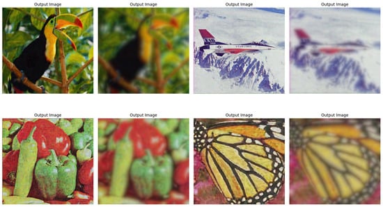
Figure 11.
Visual comparison results of denoised color images obtained by DIP-MC and DIP-TV. (first row), (second row), DIP-MC (first and third column), DIP-TV (second and fourth column).
Figure 12 shows the training behavior of the proposed DIP-MC method on a dataset of color images. The first row displays the loss curves over epochs, indicating stable convergence for all four test images. The second row presents the PSNR progression, showing that reconstruction quality steadily improves during training. The third row depicts the SSIM evolution, reflecting continuous enhancement in structural similarity to the reference images. Collectively, these plots demonstrate that DIP-MC effectively improves both quantitative metrics and perceptual quality for color images.
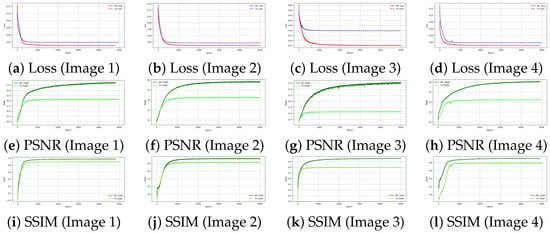
Figure 12.
Training performance of the proposed DIP-MC method on a dataset of color images. The first row presents epoch-wise loss curves, the second row shows PSNR progression throughout training, and the third row illustrates SSIM evolution. Each column corresponds to a different test image (images 1–4).
Figure 13 presents a neuron-wise parameter analysis for four representative color images (image 3, image 7, image 11, and image 15). The first row shows the neurons with the strongest contribution learned by the DIP-MC method, while the second row illustrates the corresponding results for the DIP-TV method. Each subplot highlights the best learned weights, revealing how the two approaches allocate representational capacity across different neurons. DIP-MC method emphasizes neurons that capture both spatial structures and chromatic variations, providing a more balanced distribution of representational power. In contrast, the DIP-TV method enforces smoother parameter usage, reflecting its regularization-driven learning behavior. By identifying the most influential neurons, this analysis goes beyond conventional performance measures such as loss, PSNR, and SSIM, offering deeper insights into how two methods organize their parameters during training for color image reconstruction.
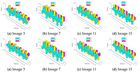
Figure 13.
Neuron-wise parameter analysis of four representative color images is shown. First and second rows correspond to the best weights learned by DIP-MC and DIP-TV methods, respectively.
4.2. Image Deblurring
In the field of image deblurring, a blurry image is generated by initially applying a blur kernel H and then adding AWGN with a noise level . The objective is to recover the original image from its impaired version. DIP-MC and DIP-TV regularization methods were evaluated using a network architecture described in [15], with . Both methods were set to operate for the same number of optimization steps. Leveraging advancements in CNNs, the blur operation using convolution was implemented. For performance comparison, the proposed DIP-MC and DIP-TV methods were used as baselines and tested on the same image dataset that was used for deblurring experiments. Two different blur kernels, a conventional Gaussian kernel with a standard deviation of 1.6 and a realistic kernel as described in [17], were employed.
4.2.1. Gaussian Deblurring: Comparative Analysis of DIP-MC and DIP-TV
In Figure 14, the first and third columns show outputs generated by DIP-MC, while the second and fourth columns present the outcomes obtained by using DIP-TV. This side-by-side comparison highlights the differences in performance between the two methods, particularly in terms of piecewise smoothness and noise reduction. The visual results demonstrate that DIP-MC achieved superior restoration quality, as evidenced by its ability to preserve finer details and enhance structural clarity compared to DIP-TV. This is consistent with the numerical enhancements noted in Table 4, where DIP-MC consistently exceeds DIP-TV in both PSNR and SSIM evaluations.
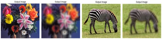
Figure 14.
Visual comparison of Gaussian deblurring results on color images obtained by DIP-MC (first and third image) and DIP-TV (second and fourth image).
Table 4.
Average PSNR and SSIM results for DIP-MC and DIP-TV methods in deblurring Gaussian blur () distorted color images tested for a period of 3000 epochs.
The findings demonstrate that DIP-MC consistently attains superior PSNR and SSIM performance when compared to DIP-TV across all images evaluated. For example, DIP-MC recorded a PSNR of 26.49 and an SSIM of 0.86, whereas DIP-TV showed a PSNR of 22.88 and an SSIM of 0.82 for image 9. This highlights the effectiveness of the multi-component regularization in DIP-MC for preserving structural details and improving image quality. On the other hand, DIP-TV showed competitive results of slightly lower performance with PSNR and SSIM values ranging from 15.52 to 22.88 and 0.70 to 0.82, respectively. These results underscore the advantages of incorporating advanced regularization techniques into the DIP framework for image deblurring tasks.
4.2.2. Motion Deblurring: Comparative Analysis of DIP-MC and DIP-TV
In the results of Figure 15, the first and third columns correspond to the outputs generated by DIP-MC, while the second and fourth columns represent the results obtained using DIP-TV. This side-by-side comparison highlights the differences in performance between the two methods, particularly in terms of restoring sharp edges and reducing artifacts caused by motion blur. The visual results demonstrate that DIP-MC achieved superior restoration quality, as evidenced by its ability to preserve finer details and enhance structural clarity compared to DIP-TV. This is consistent with the measurable enhancements noted in Table 5, where DIP-MC consistently surpasses DIP-TV regarding both PSNR and SSIM metrics.
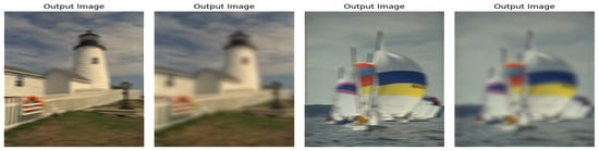
Figure 15.
Visual comparison of motion deblurring results on color images obtained by DIP-MC (first and third image) and DIP-TV (second and fourth image).
Table 5.
PSNR and SSIM averages obtained from DIP-MC and DIP-TV techniques for deblurring color images affected by motion blur (kernel size = 20, testing epochs = 3000).
Findings show that DIP-MC consistently outperforms DIP-TV in terms of PSNR and SSIM values for most of the tested images. For example, DIP-MC obtained a PSNR of 21.87 and an SSIM of 0.84 for Image 9, whereas DIP-TV recorded a PSNR of 22.42 and an SSIM of 0.82 for the same image. Although DIP-TV showed a slightly higher PSNR for Image 9, DIP-MC maintained better overall performance, particularly in terms of SSIM, which reflects its ability to preserve structural similarity and perceptual quality. On the other hand, DIP-TV showed competitive results of slightly lower performance for other images with PSNR and SSIM values ranging from 14.78 to 22.42 and 0.75 to 0.87, respectively. These results underscore the advantages of incorporating multi-component regularization in the DIP framework for motion deblurring tasks, as it effectively balances noise reduction and detail preservation.
4.3. Experimentation on Levin Dataset
The Levin dataset is employed for experimental evaluation, which is a widely recognized benchmark for blind image deconvolution and deblurring [17]. This dataset contains four high-quality ground truth images along with their synthetically blurred counterparts generated using real camera shake kernels. The availability of both sharp and blurred versions makes it suitable for rigorous quantitative evaluation of deblurring methods, particularly in terms of metrics such as PSNR and SSIM. In this work, all four ground truth images from this dataset were utilized to validate the effectiveness of the proposed DIP-MC method as shown in Figure 16.
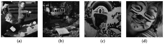
Figure 16.
Ground truth images from the Levin dataset used in validation experiments.
To further demonstrate the robustness and reconstruction quality of the proposed method, DIP-MC was compared against two well-established deblurring techniques, BM3D [18] and EPLL [19]. Quantitative results of this comparison are presented in Table 6, which clearly indicate that DIP-MC consistently achieves higher PSNR and SSIM values across all four test images, outperforming both BM3D and EPLL.
Table 6.
Quantitative comparison of PSNR and SSIM values obtained by DIP-MC, BM3D, and EPLL on the Levin dataset. Evaluation was carried out on motion-blurred images (kernel size = 20, testing epochs = 3000), resulting in superior performance of the DIP-MC method.
Qualitative comparison of deblurred images resulting from the proposed DIP-MC method, BM3D, and EPLL is presented in Figure 17. The first row shows the results of DIP-MC, where recovered images clearly preserve fine structural details, restore sharper edges, and suppress ringing artifacts more effectively than the competing methods. In contrast, the BM3D results in the second row suffer from noticeable oversmoothing, leading to loss of important texture information. EPLL outputs in the third row show successful noise reduction, but a tendency to blur high-frequency components and failure to reconstruct subtle image details. Overall, the DIP-MC method demonstrates visually superior performance by achieving a better balance between sharpness preservation and artifact suppression, thus confirming its effectiveness for blind image deblurring tasks.
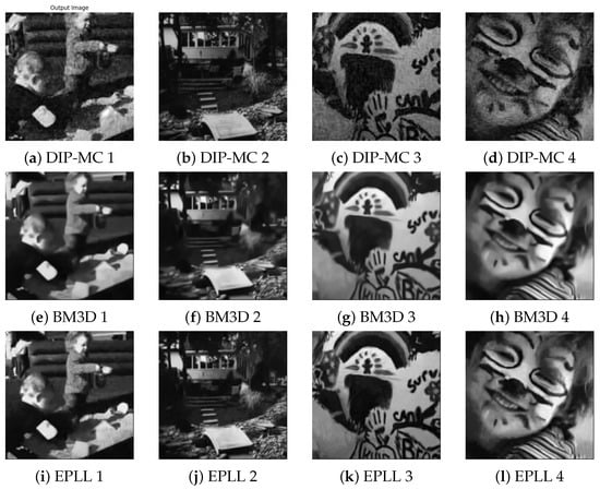
Figure 17.
Comparison of deblurring results on the Levin dataset. Rows (top to bottom) represent output from DIP-MC, BM3D, and EPLL, respectively. Each column corresponds to a different test image (1 to 4).
4.4. Analysis of Deep Image Prior Mean Curvature Based Convolutional Neural Network
In this subsection, a detailed analysis of the proposed DIP-MC-based CNN is presented. To assess the learning dynamics and stability of the network, the evolution of key performance metrics during training was investigated. In particular, epoch versus PSNR and epoch versus SSIM curves were plotted, which provide insight into how reconstruction quality improves as the number of training iterations increases. For convergence behavior and optimization process robustness evaluations, best weight plots for selected test images were also examined. These plots highlight the iterations at which the network achieves its peak performance, thereby validating the effectiveness of the DIP-MC framework in blind image deblurring tasks. In addition to analyzing the proposed method, the same plots were also generated for the previously developed DIP-TV method [15], enabling a fair comparison between the two approaches. This comparative study allows us to highlight the improvements achieved by incorporating mean curvature regularization into the DIP framework.
Figure 18 presents the training behavior of the DIP-MC network on four representative images from the Levin dataset. The first row shows the loss curves over epochs, indicating stable convergence for all images. The second row illustrates the PSNR progression, highlighting consistent improvement in reconstruction quality as the network is trained. The third row presents the SSIM evolution, reflecting increasing structural similarity between the reconstructed and ground truth images. Overall, these plots demonstrate that the DIP-MC network effectively enhances both pixel-level accuracy and perceptual quality while maintaining smooth and robust convergence across different test images.
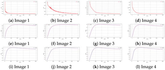
Figure 18.
Training evaluation of DIP-MC network on Levin dataset. Rows (top to bottom) show epoch-wise loss curves, PSNR progression, and SSIM evolution, respectively, for four representative images. These plots illustrate how the network gradually improves both quantitative metrics and perceptual quality during training.
Figure 19 presents a neuron-wise parameter analysis of the DIP-MC network for four representative images from the Levin dataset. Each subplot illustrates the neurons with the strongest contribution after complete training, reflecting the best learned weights. These plots reveal how the network allocates its capacity, emphasizing neurons that play a critical role in reconstructing each image. By highlighting the most influential neurons, this analysis complements conventional evaluation metrics such as loss, PSNR, and SSIM, offering deeper interpretability of the network’s internal mechanisms and the distribution of learned parameters across different images.
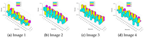
Figure 19.
Neuron-wise parameter analysis of DIP-MC network on four representative images of the Levin dataset. The plots visualize the best learned weights, highlighting the neurons that most significantly influence the network’s output for each image. This analysis provides insight into how the DIP-MC model distributes its representational capacity across different test images.
5. Conclusions
This study introduces a novel framework (DIP-MC) that combines mean curvature (MC) regularization with the deep image prior (DIP) approach for single-image restoration tasks such as denoising and deblurring. By leveraging the geometric properties of images through MC regularization, DIP-MC reduces staircasing artifacts and preserves fine structural details, effectively addressing the limitations of total variation (TV). The DIP framework is further enhanced by incorporating a self-attention block between the encoder and decoder. This allows the network to capture long-range dependencies and global contextual information, leading to improved texture and detail reconstruction.
Extensive experimentation on both grayscale and color images demonstrated that DIP-MC consistently outperformed DIP-TV in terms of peak signal-to-noise ratio (PSNR) and structural similarity index measure (SSIM), particularly under high-noise conditions. Moreover, evaluation on the Levin dataset validated the competitive performance of DIP-MC in comparison to classical methods such as BM3D and EPLL. It is important to note that the proposed method achieved high performance results without requiring large-scale datasets, making it a robust and efficient solution for single-image restoration.
The contributions of this work can be summarized as follows: (i) extending DIP with MC regularization provided a stronger geometric prior than TV; (ii) 3D weight visualizations are introduced to better understand the contribution of network parameters in denoising and deblurring tasks; (iii) competitive results were demonstrated against state-of-the-art methods on the Levin dataset; (iv) DIP-MC can effectively handle Gaussian noise and motion blur using a convolutional neural network-based framework without relying on large datasets.
In future work recommendations, further enhancement of DIP-MC is planned by incorporating fractional-order regularization methods, which offer greater flexibility in balancing smoothness and detail preservation. Development of a preconditioned optimizer is planned, which is tailored for DIP-MC, to accelerate convergence and to improve stability during training. These extensions will broaden the applicability of DIP-MC to more challenging image restoration tasks, including super-resolution, inpainting, and real-world degradation models. In this way, DIP-MC is envisioned as a scalable and high-performance framework for advanced image reconstruction.
Author Contributions
M.I.: Conceptualization, Data curation, Methodology, Writing—original draft. S.A. (Shahbaz Ahmad): Formal analysis, Investigation, Methodology, Validation, Writing—original draft. M.N.A.: Investigation, Software, Validation, Visualization, Writing—review & editing. S.A. (Saad Arif): Funding acquisition, Investigation, Project administration, Resources, Supervision, Validation, Writing—review & editing. All authors have read and agreed to the published version of the manuscript.
Funding
This work was supported by the Deanship of Scientific Research, Vice Presidency for Graduate Studies and Scientific Research, King Faisal University, Saudi Arabia [Grant No. KFU253800].
Data Availability Statement
The original data presented in the study are openly available in Kaggle (Berkeley Segmentation Dataset 68) at https://www.kaggle.com/code/mpwolke/berkeley-segmentation-dataset-68/input (accessed on 1 October 2025).
Acknowledgments
This work was supported by the Deanship of Scientific Research, Vice Presidency for Graduate Studies and Scientific Research, King Faisal University, Saudi Arabia [Grant No. KFU253800]. The authors would like to thank GC University, Lahore (GCUL), for their ongoing assistance.
Conflicts of Interest
The authors declare that they have no known competing financial interests or personal relationships that could have appeared to influence the work reported in this paper.
Abbreviations
| CNN | Convolutional Neural Network |
| TV | Total Variation |
| DIP | Deep Image Prior |
| MC | Mean Curvature |
| AWGN | Additive White Gaussian Noise |
| SGD | Stochastic Gradient Descent |
| ADAM | Adaptive Moment Estimation |
| PSNR | Peak Signal-to-Noise Ratio |
| SSIM | Structural Similarity Index Measure |
| BM3D | Block-Matching and 3D Filtering |
| EPLL | Expected Patch Log Likelihood |
| GPU | Graphics Processing Unit |
References
- Rudin, L.I.; Osher, S.; Fatemi, E. Nonlinear total variation based noise removal algorithms. Phys. D Nonlinear Phenom. 1992, 60, 259–268. [Google Scholar] [CrossRef]
- Figueiredo, M.A.T.; Nowak, R.D. Wavelet-based image estimation: An empirical bayes approach using Jeffreys’ non-informative prior. IEEE Trans. Image Process. 2001, 10, 1322–1331. [Google Scholar] [CrossRef]
- Elad, M.; Aharon, M. Image denoising via sparse and redundant representations over learned dictionaries. IEEE Trans. Image Process. 2006, 15, 3736–3745. [Google Scholar] [CrossRef]
- Danielyan, A.; Katkovnik, V.; Egiazarian, K. BM3D frames and variational image deblurring. IEEE Trans. Image Process. 2012, 21, 1715–1728. [Google Scholar] [CrossRef]
- LeCun, Y.; Bengio, Y.; Hinton, G. Deep learning. Nature 2015, 521, 436–444. [Google Scholar] [CrossRef]
- Mousavi, A.; Patel, A.B.; Baraniuk, R.G. A deep learning approach to structured signal recovery. In Proceedings of the Allerton Conference on Communication, Control, and Computing (Allerton), Monticello, IL, USA, 30 September–2 October 2015; pp. 1336–1343. [Google Scholar]
- Jin, K.H.; McCann, M.T.; Froustey, E.; Unser, M. Deep convolutional neural network for inverse problems in imaging. IEEE Trans. Image Process. 2017, 26, 4509–4522. [Google Scholar] [CrossRef] [PubMed]
- Han, Y.S.; Yoo, J.; Ye, J.C. Deep learning with domain adaptation for accelerated projection reconstruction MR. arXiv 2017, arXiv:1703.01135. [Google Scholar] [CrossRef]
- Sun, Y.; Xia, Z.; Kamilov, U.S. Efficient and accurate inversion of multiple scattering with deep learning. Opt. Express 2018, 26, 14678–14688. [Google Scholar] [CrossRef] [PubMed]
- Lee, D.; Yoo, J.; Tak, S.; Ye, J.C. Deep residual learning for accelerated MRI using magnitude and phase networks. IEEE Trans. Biomed. Eng. 2018, 65, 1985–1995. [Google Scholar] [CrossRef] [PubMed]
- Meinhardt, T.; Moeller, M.; Hazirbas, C.; Cremers, D. Learning proximal operators: Using denoising networks for regularizing inverse imaging problems. In Proceedings of the 2017 IEEE International Conference on Computer Vision (ICCV), Venice, Italy, 22–29 October 2017; pp. 1799–1808. [Google Scholar]
- Zhang, K.; Zuo, W.; Gu, S.; Zhang, L. Learning deep CNN denoiser prior for image restoration. In Proceedings of the 2017 IEEE Conference on Computer Vision and Pattern Recognition (CVPR), Honolulu, HI, USA, 21–26 July 2017. [Google Scholar]
- Romano, Y.; Elad, M.; Milanfar, P. The little engine that could: Regularization by denoising (RED). SIAM J. Imaging Sci. 2017, 10, 1804–1844. [Google Scholar] [CrossRef]
- Sun, Y.; Wohlberg, B.; Kamilov, U.S. An Online Plug-and-Play Algorithm for Regularized Image Reconstruction. IEEE Trans. Comput. Imaging 2018, 4, 187–199. [Google Scholar] [CrossRef]
- Ulyanov, D.; Vedaldi, A.; Lempitsky, V. Deep image prior. In Proceedings of the IEEE Conference on Computer Vision and Pattern Recognition (CVPR), Salt Lake City, UT, USA, 18–22 June 2018; pp. 9446–9454. [Google Scholar]
- Van Veen, D.; Jalal, A.; Price, E.; Vishwanath, S.; Dimakis, A.G. Compressed Sensing with Deep Image Prior and Learned Regularization. In Proceedings of the 36th International Conference on Machine Learning, Long Beach, CA, USA, 9–15 June 2019; pp. 1–10. [Google Scholar]
- Levin, A.; Weiss, Y.; Durand, F.; Freeman, W.T. Understanding and evaluating blind deconvolution algorithms. In Proceedings of the 2009 IEEE Conference on Computer Vision and Pattern Recognition, Miami, FL, USA, 20–25 June 2009; IEEE: Piscataway, NJ, USA, 2009; pp. 1964–1971. [Google Scholar] [CrossRef]
- Dabov, K.; Foi, A.; Katkovnik, V.; Egiazarian, K. Image denoising by sparse 3-D transform-domain collaborative filtering. IEEE Trans. Image Process. 2007, 16, 2080–2095. [Google Scholar] [CrossRef]
- Zoran, D.; Weiss, Y. Learning patch priors for denoising and deblurring. In Proceedings of the 2011 International Conference on Computer Vision, Barcelona, Spain, 6–13 November 2011; IEEE: Piscataway, NJ, USA, 2011; pp. 323–330. [Google Scholar]
- Boucherit, I.; Kheddar, H. Reinforced Residual Encoder–Decoder Network for Image Denoising via Deeper Encoding and Balanced Skip Connections. Big Data Cogn. Comput. 2025, 9, 82. [Google Scholar] [CrossRef]
- Liang, J.; Cao, J.; Sun, G.; Zhang, K.; Van Gool, L.; Timofte, R. SwinIR: Image Restoration Using Swin Transformer. In Proceedings of the IEEE/CVF International Conference on Computer Vision (ICCV) Workshops, Virtually, 11–17 October 2021; pp. 1833–1844. [Google Scholar]
- Zamir, S.W.; Arora, A.; Khan, S.; Hayat, M.; Khan, F.S.; Yang, M.H.; Shao, L. Restormer: Efficient Transformer for High-Resolution Image Restoration. In Proceedings of the IEEE/CVF Conference on Computer Vision and Pattern Recognition (CVPR), New Orleans, LA, USA, 19–24 June 2022; pp. 5728–5739. [Google Scholar]
- Anwar, S.; Barnes, N. Densely connected multi-dilated convolutional network for image denoising. IEEE Trans. Image Process. 2022, 31, 4610–4625. [Google Scholar]
- Liu, J.; Sun, Y.; Xu, X.; Kamilov, U.S. Image restoration using total variation regularized deep image prior. In Proceedings of the ICASSP 2019—2019 IEEE International Conference on Acoustics, Speech and Signal Processing (ICASSP), Brighton, UK, 12–17 May 2019; IEEE: Piscataway, NJ, USA, 2019; pp. 7715–7719. [Google Scholar]
- Khalid, R.; Ahmad, S.; Ali, I.; De la Sen, M. Enhanced BiCGSTAB with Restrictive Preconditioning for Nonlinear Systems: A Mean Curvature Image Deblurring Approach. Math. Comput. Appl. 2025, 30, 76. [Google Scholar] [CrossRef]
- Mobeen, A.; Ahmad, S.; Fairag, F. Non-blind constraint image deblurring problem with mean curvature functional. Numer. Algorithms 2025, 98, 1703–1723. [Google Scholar] [CrossRef]
- Iqbal, A.; Ahmad, S.; Kim, J. Two-Level method for blind image deblurring problems. Appl. Math. Comput. 2025, 485, 129008. [Google Scholar] [CrossRef]
- Saleem, S.; Fairag, F.; Al-Mahdi, A.M.; Al-Gharabli, M.M.; Ahmad, S. Conformable fractional order variation-based image deblurring. Partial Differ. Equ. Appl. Math. 2024, 11, 100827. [Google Scholar] [CrossRef]
- Kim, J.; Ahmad, S. On the preconditioning of the primal form of TFOV-based image deblurring model. Sci. Rep. 2023, 13, 17422. [Google Scholar] [CrossRef]
- Zhang, K.; Zuo, W.; Zhang, L. IRCNN++: Improved Regularization-Based Convolutional Network for Image Restoration. IEEE Trans. Image Process. 2023, 32, 1852–1864. [Google Scholar]
- Li, X.; Chen, H.; Wang, Y. Attention-Guided Deep Residual Network for Image Deblurring. Pattern Recognit. Lett. 2023, 167, 23–31. [Google Scholar]
- Wang, R.; Liu, Y.; Chen, T. RestFormer: Transformer-Based Image Restoration with Enhanced Spatial Attention. IEEE Access 2024, 12, 56120–56132. [Google Scholar]
- Ducotterd, S.; Neumayer, S.; Unser, M. Learning a Convex Patch-Based Synthesis Model via Deep Equilibrium. In Proceedings of the ICASSP 2024—2024 IEEE International Conference on Acoustics, Speech and Signal Processing (ICASSP), Seoul, Republic of Korea, 14–19 April 2024; pp. 2031–2035. [Google Scholar] [CrossRef]
- Zhang, J.; Tu, Y. SwinFR: Combining SwinIR and fast fourier for super-resolution reconstruction of remote sensing images. Digital Signal Process. 2025, 159, 105026. [Google Scholar] [CrossRef]
- Feng, H.; Zhou, H.; Ye, T.; Chen, S.; Zhu, L. Residual Diffusion Deblurring Model for Single Image Defocus Deblurring. In Proceedings of the AAAI Conference on Artificial Intelligence, Philadelphia, PA, USA, 25 February–4 March 2025; pp. 2960–2968. [Google Scholar] [CrossRef]
- Zhu, W.; Chan, T. Image Denoising Using Mean Curvature of Image Surface. SIAM J. Imaging Sci. 2012, 5, 1–32. [Google Scholar] [CrossRef]
- Bertalmío, M.; Sapiro, G.; Cheng, L.T.; Caselles, V. Image Inpainting. In Proceedings of the 27th International Conference on Computer Graphics and Interactive Techniques Conference, New Orleans, LA, USA, 23–28 July 2000; pp. 417–424. [Google Scholar] [CrossRef]
- Egmont-Petersen, M.; de Ridder, D.; Handels, H. Image Processing with Neural Networks—A Review. Pattern Recognit. 2002, 35, 2279–2301. [Google Scholar] [CrossRef]
- Xie, J.; Xu, L.; Chen, E. Image Denoising and Inpainting with Deep Neural Networks. In Proceedings of the Advances in Neural Information Processing Systems (NeurIPS), Lake Tahoe, NV, USA, 3–6 December 2012; pp. 341–349. [Google Scholar]
- Zhang, K.; Zuo, W.; Chen, Y.; Meng, D.; Zhang, L. Beyond a Gaussian Denoiser: Residual Learning of Deep CNN for Image Denoising. IEEE Trans. Image Process. 2017, 26, 3142–3155. [Google Scholar] [CrossRef]
- Kingma, D.P.; Ba, J. Adam: A Method for Stochastic Optimization. arXiv 2014, arXiv:1412.6980. [Google Scholar]
- Ronneberger, O.; Fischer, P.; Brox, T. U-Net: Convolutional Networks for Biomedical Image Segmentation. In Proceedings of the International Conference on Medical Image Computing and Computer-Assisted Intervention (MICCAI), Munich, Germany, 5–9 October 2015; Springer: Cham, Switzerland, 2015; pp. 234–241. [Google Scholar]
Disclaimer/Publisher’s Note: The statements, opinions and data contained in all publications are solely those of the individual author(s) and contributor(s) and not of MDPI and/or the editor(s). MDPI and/or the editor(s) disclaim responsibility for any injury to people or property resulting from any ideas, methods, instructions or products referred to in the content. |
© 2025 by the authors. Licensee MDPI, Basel, Switzerland. This article is an open access article distributed under the terms and conditions of the Creative Commons Attribution (CC BY) license (https://creativecommons.org/licenses/by/4.0/).