An Enhanced Tuna Swarm Algorithm for Link Scheduling Strategies in Wireless Sensor Networks

Abstract

In resource-constrained wireless sensor networks, efficient link scheduling is a well-studied challenge. This problem is NP-hard, indicating that NP (Nondeterministic Polynomial Time) refers to problems whose solutions can be verified in polynomial time but are computationally difficult to find, and traditional methods seldom yield optimal solutions within practical time limits. This research introduces an innovative novel link scheduling strategy based on the Tuna Swarm Optimization (TSO-LS) algorithm to optimize the link scheduling performance of wireless sensor networks. This work enhances the tuna swarm algorithm’s search process by incorporating characteristics of the link scheduling problem, resulting in specialized algorithmic improvements for this scenario. This research presents three principal improvements to the algorithm: first, optimizing the individual update mechanism to expedite scheduling solutions; second, refining the leading individual selection strategy to elevate global scheduling quality; and third, maintaining population diversity to prevent convergence on suboptimal scheduling schemes. In the experimental section, TSO-LS is compared with the Genetic Algorithm, Particle Swarm Optimization, Enhanced Particle Swarm Optimization and Ant Colony Optimization. The results show that TSO-LS achieves a 13.3% improvement in energy efficiency and a 12.5% decrease in average latency. Under different experimental conditions, the TSO-LS strategy shortens the average latency to 10.5 ms, demonstrating outstanding overall performance. Furthermore, this strategy reduces node consumption from 0.41 mJ to 0.32 mJ, significantly extending the overall lifespan of the network.

1. Introduction

Wireless Sensor Networks (WSNs) serve as fundamental infrastructure for diverse applications such as precision agriculture and industrial automation, where reliable data transmission is crucial. The central challenge in these systems lies in resolving the inherent conflict between concurrent transmission efficiency and interference management during link scheduling. This dilemma becomes particularly acute in dense deployments where improper scheduling directly accelerates energy depletion and compromises network longevity. These resource constraints further intensify the scheduling predicament, creating a pressing need for optimized scheduling strategies that can balance transmission demands with sustainable resource utilization [1,2]. Among these challenges, efficient link scheduling is paramount, directly impacting data transmission reliability, network longevity, and overall Quality of Service (QoS). The problem of optimizing link scheduling in WSNs is inherently complex and often falls into the category of NP-hard problems [3], making it difficult for traditional methods to find optimal solutions within a reasonable timeframe.

For a considerable period, extensive research has leveraged bio-inspired metaheuristics to tackle these challenges, focusing on enhancing routing, connectivity, and resource utilization in WSNs. Ant Colony Optimization (ACO), for instance, has been a prominent choice, with early investigations introducing ACO-based routing protocols to optimize data transmission paths and enhance link efficiency [4]. Subsequent advancements include approaches for determining mobile sink paths to extend network lifespan and optimize link connections [5], as well as secure ACO routing algorithms for IoT environments that emphasize link reliability and security [6]. Similarly, Particle Swarm Optimization (PSO) has been widely adopted due to its efficiency, having been comprehensively reviewed for its applications in link coverage and energy optimization [7]. More recent contributions include PSO-based amorphous algorithms for reducing localization errors to improve link accuracy [8], and PSO scheduling techniques designed to maximize network lifespan by optimizing link energy consumption [9]. Genetic Algorithm (GA) also represents a significant class of metaheuristics applied to WSN link optimization, with notable works including methods for improving sensor deployment to enhance coverage and link connectivity [10], reviews summarizing GA applications in wireless networks [11], and GA-based routing game algorithms addressing multi-objective optimization through link quality [12]. Beyond these bio-inspired approaches, recent research has also explored deterministic and adaptive techniques, such as approximation-based shortest link scheduling with power control [13], SINR (Signal-to-Interference-plus-Noise Ratio)-based slot reuse algorithms for multi-channel WSNs [14], consensus estimation for enhanced effectiveness [15], and adaptive filtering-based self-calibration methods [16].

While these established methods have significantly advanced WSN link scheduling, providing robust solutions for various optimization objectives, they often face inherent limitations when confronted with the dynamic and complex nature of WSNs [2]. Bio-inspired algorithms, despite their effectiveness, can be prone to premature convergence, get trapped in local optima, or suffer from slower convergence speeds when dealing with high-dimensional and dynamic link scheduling problems [2]. For example, ACO can be computationally intensive for large networks, and PSO might struggle with multimodal objective functions, potentially leading to suboptimal solutions in complex WSN environments [17]. Deterministic and adaptive techniques, while offering precision, may struggle with scalability in large-scale WSNs, require extensive computational resources, or exhibit reduced adaptability to rapidly changing network conditions and interference patterns [18]. These limitations underscore the continuous need for novel optimization paradigms that can offer improved performance, robustness, and adaptability in the face of evolving WSN complexities.

Tuna Swarm Algorithm (TSA), a relatively novel bio-inspired metaheuristic, draws its inspiration from the sophisticated foraging behaviors of tuna schools, including their distinctive spiral and parabolic foraging strategies [19]. Introduced in recent years, TSA, as a swarm intelligence technique, has rapidly gained recognition for its robust global search capabilities and commendable convergence speed, rendering it highly suitable for addressing complex optimization problems across diverse scientific and engineering domains [20]. Initial investigations primarily focused on validating the approach through benchmark function optimization and its application to various engineering design challenges, showcasing superior performance compared to established algorithms such as PSO and ACO [19]. Subsequent advancements have led to hybrid variants designed to achieve a better balance between exploration and exploitation [21]. In practical application domains, TSA has proven adaptable for intricate resource allocation and scheduling problems, including optimizing energy consumption in cloud computing [22], antenna array optimization in wireless communication systems [23], and node clustering in IoT and sensor networks [24].

Despite these promising applications and TSA’s inherent strengths in handling complex optimization landscapes, a significant research gap persists: the comprehensive and dedicated exploration of TSA for direct link scheduling optimization in WSNs remains largely unaddressed. Although the TSA has demonstrated potential in related areas, such as node clustering, its specific application to the multifaceted challenges of WSN link scheduling—which involve intricate considerations, including interference mitigation, dynamic topology changes, and multi-objective optimization for latency and energy efficiency—has not been thoroughly investigated. This lack of dedicated research represents a deficiency in leveraging TSA’s full potential within this critical domain, especially given its potential to overcome some of the aforementioned limitations of existing metaheuristics by offering a better balance between exploration and exploitation and potentially faster convergence for specific problem structures.

Therefore, this paper aims to bridge this gap by introducing a novel approach that specifically tailors the TSA to the unique constraints and demands of WSN link optimization. By leveraging the adaptive foraging mechanisms of the tuna swarm algorithm, this study aims to develop a robust solution, termed Tuna Swarm Optimization for Link Scheduling (TSO-LS), which is capable of optimizing link allocation, effectively reducing latency, and significantly enhancing energy efficiency in WSNs. This approach addresses the limitations of previous generalized applications and presents a specialized, high-performance optimization paradigm for this critical area. The proposed TSO-LS algorithm integrates the search mechanism of the tuna swarm algorithm with the characteristics of the link scheduling problem and further designs algorithmic improvements tailored to this scenario.

The remainder of this paper is organized as follows: Section 2 presents the related work. Section 3 describes the network model and the link scheduling problem formulation. Section 4 details the proposed TSO-LS algorithm, including its enhanced mechanisms. Section 5 presents the experimental setup and discusses the performance evaluation results. Finally, Section 6 concludes the paper and outlines future research directions.

2. Related Work

2.1. Link Scheduling Approaches

Optimizing link scheduling in WSNs is essential for effective data transfer and prolonged network lifespan. For an extended duration, substantial research has utilized bio-inspired metaheuristics to address these difficulties. Research concentrates on improving routing, connectivity, and resource efficiency. Among these, ACO has emerged as a significant option. Preliminary studies, for example, presented a routing system based on ACO. This protocol seeks to optimize data transmission routes and improve link efficiency in wireless sensor networks. Subsequent innovations encompass Kumar et al.’s methodology, which identifies mobile sink trajectories to prolong network longevity and enhance link connectivity [5]. An additional instance is a secure ACO routing algorithm tailored for IoT contexts. This approach prioritizes the dependability and security of links [6]. Likewise, PSO has been extensively utilized owing to its efficacy. Kulkarni et al.’s extensive survey, for example, examined its implementation in link coverage and energy optimization [7]. Recent advances encompass PSO-based amorphous algorithms designed to mitigate localization problems and enhance link accuracy and connectivity [8]. PSO scheduling algorithms have been developed to enhance network longevity by optimizing energy consumption of links [9]. GA constitutes a notable category of metaheuristics utilized for link optimization in WSN. Significant contributions encompass Tossa et al.’s approach for optimizing sensor placement to augment coverage and link connectivity [10]. Shahi et al.’s review encapsulates the uses of genetic algorithms in wireless networks, encompassing link optimization in wireless sensor networks. The GA-based routing game technique by Hao et al. tackles multi-objective optimization via link quality [12].

Beyond these bio-inspired approaches, recent and contemporary research has also delved into deterministic and adaptive techniques for link scheduling. For instance, Mohammadi et al. proposed the PDSLS algorithm, which employs approximation-based shortest link scheduling with power control to minimize latency [13]. Zeng et al. developed an SINR-based slot reuse algorithm for multi-channel WSNs, optimizing resource allocation [14]. Tian et al.’s study enhances WSN effectiveness by leveraging consensus estimation and universal coverage [15], while an adaptive filtering-based self-calibration method refines link scheduling by dynamically adjusting to environmental variations [16].

These studies demonstrate an extension of the network lifetime, as shown in Table 1. The lifetime of the network is defined as the duration from the commencement of network operation until the ratio of failing nodes attains a predetermined threshold (e.g., 100%). In WSN investigations, the number of rounds is frequently utilized as an indicator of network lifetime [25]. The reported survival rounds should be considered reference values solely, given the experiments were performed under varying network setups. The percentage improvement attained by the algorithm in identical cases is of more importance.

Table 1. Lifetime of WSNs Using Different Algorithms.

Algorithm Category	Algorithm Name	Network Lifetime
ACO-based	ACO Basic Routing [4]	10% improvement compared to EEABR
	ACO Mobile Sink [5]	40–150% longer than WRP(uniform)
PSO-based	PSO Lifetime Max [9]	1800 rounds, 50% higher than PSOK
GA-based	GABLQ (Link Quality) [12]	1428 rounds, 16.8% higher than LEACH-IMPT
Traditional	LEACH	100 rounds
	LEACH-IMPT	600 rounds
	NWPSO	837 rounds
	PSOK	1200 rounds

These diverse developments collectively address critical challenges such as interference, energy efficiency, and scalability inherent in WSN link scheduling.While these established methods have significantly advanced WSN link scheduling, providing robust solutions for various optimization objectives, the dynamic and complex nature of WSNs continually presents new challenges and opportunities for novel optimization paradigms.

2.2. Emerging Trends and Nascent Works

Beyond the classical bio-inspired approaches discussed above, the landscape of link scheduling has recently evolved towards more complex and intelligent paradigms. A significant body of nascent work focuses on Hybrid Metaheuristics, which combine multiple algorithms to avoid local optima. For instance, Kapoor and Sharma [26] recently proposed a hybrid model integrating PSO, GA, and Grey Wolf Optimization (GWO) to balance clustering and sleep scheduling, demonstrating superior convergence compared to single-mechanism algorithms.

Simultaneously, Machine Learning (ML) and Deep Reinforcement Learning (DRL) have emerged as powerful tools for dynamic scheduling. Yuan et al. [27] introduced a DRL-based framework that enables sensor nodes to autonomously learn energy-efficient transmission strategies through interaction with the environment, significantly outperforming static schedules in highly dynamic topologies. Similarly, in industrial settings, enhanced scheduling algorithms for Time-Slotted Channel Hopping (TSCH) have been developed to guarantee deterministic latency [28].

While these learning-based and hybrid methods offer impressive performance, they often entail high computational complexity and training overheads that may burden resource-constrained sensor nodes. In contrast, the TSA has continued to evolve as a lightweight yet efficient solution. Recent studies in 2025 have further expanded TSA’s capabilities to complex engineering domains. Khiar et al. [29] successfully applied a Binary TSA to discrete feature selection problems, while Wang et al. [30] proposed a Fast Non-Dominated Sorting TSA for multi-objective time-energy optimization. These nascent works, alongside recent applications in node localization [31], validate that improved TSA mechanisms can strike an optimal balance between the high search efficiency required for modern networks and the low computational cost demanded by practical WSN hardware.

2.3. Tuna Swarm Optimization Approaches

TSA, a relatively novel bio-inspired metaheuristic, draws its inspiration from the sophisticated foraging behaviors of tuna schools, including their distinctive spiral and parabolic foraging strategies [19]. Introduced in recent years, TSA, as a swarm intelligence technique, has rapidly gained recognition for its robust global search capabilities and commendable convergence speed, rendering it highly suitable for addressing complex optimization problems across diverse scientific and engineering domains.

Initial investigations into TSA primarily focused on its validation through benchmark function optimization and its application to various engineering design challenges. For instance, Xie et al., in their seminal work, proposed the original TSA framework, rigorously validated its efficacy on standard test functions, and showcased its superior performance in terms of accuracy and efficiency when compared to established algorithms like PSO and ACO [19]. Subsequent advancements have led to the development of hybrid variants, such as an improved TSA integrated with differential evolution, designed to achieve a better balance between exploration and exploitation in unconstrained optimization tasks [21].

In practical application domains, TSA has proven adaptable for intricate resource allocation and scheduling problems. Notable examples include its successful deployment in optimizing energy consumption within cloud computing environments, where TSA-based task scheduling effectively minimizes makespan and power usage [22]. Furthermore, in wireless communication systems, TSA has been employed for antenna array optimization, contributing to enhanced signal quality and reduced interference [23]. Emerging applications also extend to IoT and sensor networks, such as TSA-driven node clustering aimed at improving data aggregation efficiency [24].

Despite these promising applications and TSA’s inherent strengths in handling complex optimization landscapes, a significant research gap persists: the comprehensive and dedicated exploration of TSA for direct link scheduling optimization in WSNs remains largely unaddressed. While the TSA has shown promise in related areas, such as node clustering, its specific application to the multifaceted challenges of WSN link scheduling—which involve intricate considerations, including interference mitigation, dynamic topology changes, and multi-objective optimization for latency and energy efficiency—has not been thoroughly investigated. This lack of dedicated research represents a deficiency in leveraging TSA’s full potential within this critical domain.

Therefore, this paper aims to bridge this gap by introducing a novel approach that specifically tailors the Tuna Swarm Algorithm to the unique constraints and demands of WSN link optimization. By harnessing the adaptive foraging mechanisms of TSA, this study aims to develop a robust solution that optimizes link allocation, effectively reduces latency, and significantly enhances energy efficiency in WSNs. This approach addresses the limitations of previous generalized applications and provides a specialized, high-performance optimization paradigm for this critical area.

3. Preparation Work

3.1. Network Topology Model

Assume that WSNs consist of n sensor nodes randomly distributed within a square region with side length S, i.e., the area size is $S\times S$ square meters. The position of each node is represented by two-dimensional coordinates $\left(x_i,y_i\right)$, where $i=1,2,\cdots ,n$. The communication range of each node is a fixed value R. When the Euclidean distance between two nodes $d_{ij}=\sqrt{{\left(x_i-x_j\right)}^2+{\left(y_i-y_j\right)}^2}$ is less than or equal to R, there exists a potential communication link between these two nodes [13]. In this way, the adjacency matrix A of the network can be constructed: if a link exists between node i and node j, then $A_{ij}=A_{ji}=1$ otherwise, $A_{ij}=A_{ji}=0$.

In the network topology model, the network node is denoted as v. A communication link is represented by l. The scheduling solution, denoted as s, is defined as a set of links.

3.2. Node Energy of WSNs

The energy of sensor nodes is a finite and non-replenishable resource. Therefore, energy consumption must be considered during the link scheduling process. The energy consumption of a node primarily includes energy expended for data transmission, data reception, and energy loss during idle states. In the model of this paper, the focus is on the energy consumption during data transmission, as expressed by the following formula:

$$E=L·\left(E_{elec}+E_{amp}·d^2\right)$$

(1)

Here, E represents the energy consumed to transmit a data packet of length L. $E_{elec}$ is the energy consumption of the circuit for processing per bit of data; $E_{amp}$ is the energy consumption per bit per square meter of the power amplifier; and d is the transmission distance. It can be observed that energy consumption is proportional to the square of the transmission distance. Hence, during link scheduling, nodes that are closer in distance should be selected for communication as much as possible to reduce energy consumption.

3.3. Link Scheduling Model

This section presents a multi-constraint, multi-objective link scheduling model. The model explicitly quantifies the trade-off between energy consumption and packet delay. It facilitates the generation of scheduling solutions that achieve optimal balance between these competing metrics. In subsequent sections, this model will serve as the foundation for developing solution approaches. These approaches will navigate the complex solution space to produce scheduling schemes that balance these critical, interdependent performance indicators.

The link scheduling scheme is represented in the form of a binary vector, where the length of the vector equals the total number of potential links M in the network. Each element in the vector corresponds to one link. If the element value is 1, it indicates that the link is activated in the current scheduling period; if the element value is 0, it indicates that the link is not activated. For example, for a network containing M links, the scheduling scheme is $s=[s_1,s_2,\cdots ,s_M]$, where $s_i\in \{0,1\}$ and $i=1,2,\cdots ,M$.

In order to prevent nodes from participating in excessive communication links simultaneously, which would lead to excessive energy consumption and communication conflicts, each node can participate in at most one link within the same scheduling period. That is, for any node v, the following condition must be satisfied:

$$\sum _{i:v\in l_i}{s}_i\le 1$$

(2)

Here, $l_i$ denotes the i-th link.

A link scheduling objective function is established with the goals of minimizing the total network energy consumption and the packet loss rate.

Assume the communication energy consumption between node i and node j is $E_{ij}$. Then, the total energy consumption can be expressed as:

$$E_{total}=\sum _{i=1}^N\sum _{j=1,j\ne i}^N{E}_{ij}$$

(3)

Among them, the calculation formula for $E_{ij}$ may depend on the communication distance $d_{ij}$ and the communication rate $r_{ij}$, namely:

$$E_{ij}=f\left(d_{ij},r_{ij}\right)$$

(4)

Here, f is a function that describes the relationship between energy consumption and communication distance and rate.

The total energy consumption $E_{total}$ can be obtained by summing the energy consumption of all activated links. Substituting Equation (1) into Equation (2) yields:

$$E_{total}=\sum _{i=1}^M{s}_i·L·\left(E_{elec}+E_{amp}·d_i^2\right)$$

(5)

where $d_i$ is the distance between the two nodes of the i-th link.The formula for average energy consumption is $E_{total}/N$.

The packet loss rate $P_{loss}$ is closely related to factors such as link quality and interference. In the model of this paper, a distance-based packet loss rate model and packet loss due to interference are considered. For the i-th link, its base packet loss rate is $P_{base,i}=0.01·{\displaystyle \frac{d_i}{R}}$, and the packet loss rate caused by interference $P_{interference,i}$ is determined by calculating the interference level from other activated links on this link. When the minimum distance between two links is less than ${\displaystyle \frac{R}{2}}$, interference occurs. For each interfering link, the packet loss rate increases by 0.02. Thus, the total packet loss rate for the i-th link is $P_{total,i}=P_{base,i}+P_{interference,i}$, and the overall network packet loss rate is:

$$P_{loss}={\displaystyle \frac{1}{N_{active}}}\sum _{i=1}^M{s}_i·P_{total,i}$$

(6)

where $N_{active}$ is the number of activated links.

Additionally, to ensure the reliability of data transmission, the packet loss rate must also be considered. Denoting the packet loss rate of data sent by node i as $L_i$, the overall packet loss rate of the entire network can be expressed as:

$$L_{\mathrm{total}}=\sum _{i=1}^N{L}_i$$

(7)

The final objective function is:

$$\left\{\begin{array}{c}min\alpha ·E_{total}+\left(1-\alpha \right)·P_{loss}\\ s.t.\\ \sum _{i:v\in l_i}{s}_i\le 1,\\ P_{loss}\le \lambda ,\\ L_{total}\le ϵ\end{array}\right.$$

(8)

where $\alpha$ is a weighting coefficient used to balance the importance of the two objectives, energy consumption and packet loss rate, with $0\le \alpha \le 1$.The first constraint ensures the rational allocation of node communication resources, while $\lambda$ represents the maximum allowable packet loss rate. The second constraint guarantees the communication quality of the network. $ϵ$ is the maximum allowable packet loss rate.

4. Materials and Methods

4.1. Tuna Swarm Optimization Algorithm

The TSA is a novel metaheuristic algorithm inspired by the collective foraging behavior of tuna schools in the ocean. This algorithm primarily simulates the process through which a tuna school locates and captures prey using two unique cooperative strategies: spiral foraging and parabolic foraging. Spiral foraging mimics the fish school forming a tight spiral formation around the prey for large-scale movement, demonstrating strong global exploration capability. Parabolic foraging, on the other hand, simulates the fish school encircling the prey within a constantly shrinking parabolic-shaped area for meticulous local exploitation. By skillfully balancing these two strategies, TSO can efficiently search within complex solution spaces, avoid premature convergence, and ultimately find high-quality global optimum solutions.This section presents the detailed procedures of the standard TSA, while the enhanced version will be introduced in the following section.

The detailed steps of the TSA are as follows:

• Step 1: Algorithm Initialization.
  Assume that in a D-dimensional search space, there are N tunas. The position of the i-th tuna at iteration t is denoted as:

  $$X_i^t=\left(x_{i1}^t,x_{i2}^t,\dots ,x_{iD}^t\right)$$

  (9)
  The population positions are randomly initialized within the search space:

  $$X_i^0=LB+rand·(UB-LB)$$

  (10)

  where $LB$ and $UB$ are the lower bound and upper bound vectors of the search space, respectively, and $rand$ is a random number within the range [0, 1].
• Step 2: Iteration Process.
  $T_{max}$ represents the maximum number of iterations. From iteration $t=1$ to $T_{max}$, the following steps are repeated:

  -

  Step 2.1: Update Control Parameters.

  First, calculate the current parameter ${\alpha }_1$, which increases linearly from the constant value ${\alpha }_0$ to 1 as iterations progress, thereby balancing exploration and exploitation. Here, a is a constant used to control subsequent spiral movements.

  $${\alpha }_1={\alpha }_0+(1-{\alpha }_0)·{\displaystyle \frac{t}{T_{max}}}$$

  (11)

  Simultaneously, compute the parameter p used in parabolic foraging:

  $$p={(1-{\displaystyle \frac{t}{T_{max}}})}^{t/T_{max}}$$

  (12)

  -

  Step 2.2: Position Update.

  For each tuna individual i in the population, generate a random number $rand$ in the range [0, 1], and select a foraging strategy based on its value.

  Case A: Spiral Foraging (When $rand<{\displaystyle \frac{t}{T_{max}}}$)

  In this mode, the tuna moves towards the best individual $X_{\mathrm{best}}$ and a selected leader individual $X_{\mathrm{leader}}$. First, calculate ${\beta }_0$ according to the following formula, where l and b are random numbers:

  $${\beta }_0=e^{bl}·cos\left(2\pi b\right)$$

  (13)

  Then, determine the leading individual:

  $$X_{\mathrm{leader}}^t=\left\{\begin{array}{cc}{X}_i^t,\hfill & \mathrm{if}i=1\hfill \\ X_{i-1}^t,\hfill & \mathrm{if}i=2,3,\dots ,N\hfill \end{array}\right.$$

  (14)

  Finally, the position update formula for the tuna population is given as follows:

  $$X_i^{t+1}={\alpha }_1·\left(X_{\mathrm{best}}^t+{\beta }_0·\left|X_{\mathrm{best}}^t-X_i^t\right|\right)+{\alpha }_2·X_{\mathrm{leader}}^t$$

  (15)

  where $X_{\mathrm{best}}^t$ is the best individual from the i-th iteration, and $X_{\mathrm{leader}}$ is the leading individual. Formula (15) means that its position update depends entirely on the global best individual $X_{\mathrm{best}}$ and its own current position. It can be regarded as a leading individual exploring near the best position and its own current location.

  Case B: Parabolic Foraging (When $rand\ge {\displaystyle \frac{t}{T_{max}}}$)

  During this phase, the tuna forms a parabolic encirclement with the best individual as the focus. First, generate a random direction factor $TF$:

  $$TF=\left\{\begin{array}{cc}1,\hfill & \mathrm{if}rand<0.5\hfill \\ -1,\hfill & \mathrm{if}rand\ge 0.5\hfill \end{array}\right.$$

  (16)

  Then, based on another random number $randb$, select the position update method:

  if $randb<0.5$:

  $$X_i^{t+1}=X_{\mathrm{best}}^t+randc·\left(X_{\mathrm{best}}^t-X_i^t\right)+TF·p^2·\left(X_{\mathrm{best}}^t-X_i^t\right)$$

  (17)

  where $randc$ is a random number within the range [0, 1].

  if $randb\ge 0.5$:

  $$X_i^{t+1}=TF·p^2·X_i^t$$

  (18)

  -

  Step 2.3: Boundary Handling.

  Check whether the new position $X_i^{t+1}$ remains within the search boundaries $[LB,UB]$. If it exceeds the boundaries, clamp it to the boundary values.

  -

  Step 2.4: Evaluation and Selection.

  Calculate the fitness values of the new positions for all tuna individuals. If the new position of any tuna yields a better fitness value, replace its old position with the new one. Subsequently, update the global best individual $X_{\mathrm{best}}$ for the entire population.

• Step 3: Algorithm Termination.
  When the iteration counter t reaches $T_{max}$, the algorithm stops. The output $X_{\mathrm{best}}$ at this point represents the global optimal solution found by the algorithm.

4.2. TSO-LS Algorithm

Through the mathematical model established in Section 3.3, the link scheduling problem in wireless sensor networks can be transformed into an optimization problem. We design a novel link scheduling strategy based on the Tuna Swarm Optimization (TSO-LS) to solve this problem, aiming to effectively find optimal or near-optimal link scheduling schemes. This approach is expected to reduce energy consumption in wireless sensor networks and enhance overall network performance.

The core idea of TSO-LS is to map the foraging behavior of the tuna swarm to a search process within the link scheduling solution space, thereby finding a near-optimal scheduling solution that effectively balances energy consumption and packet loss rate. In the algorithm, each tuna represents a complete link scheduling solution, with each dimension corresponding to a constrained variable.

The fitness function serves as the guiding mechanism of the algorithm, evaluating the quality of each scheduling solution. We design the fitness function based on Formula (8) as follows:

$$Fitness=B_{Fitness}-\alpha ·E_{\mathrm{total}}-(1-\alpha )·P_{\mathrm{loss}}$$

(19)

where $B_{Fitness}$ is a constant. During computation, the variables $E_{total}$ and $P_{loss}$ in Equation (19) were normalized by dividing them by their respective maximum values, yielding values within the [0, 1] range.

The procedure of TSO-LS follows the same steps as TSA outlined in Section 4.1, with the following improvements introduced:

1.

Optimization of the individual update mechanism for accelerated scheduling solution; To rapidly obtain high-quality link scheduling schemes, the individual update mechanism of the algorithm has been optimized. Specifically, an adaptive weighting factor is introduced, whose value is dynamically adjusted based on the current iteration count. This effectively accelerates the algorithm’s convergence in the search through the link scheduling solution space. The calculation formula for the weighting factor is:

$$w_{t+1}={\displaystyle \frac{1}{1+e^{-w_t·w_0}}}·w_t$$

(20)

$${\alpha }_{1,t}={\alpha }_0+(1-{\alpha }_0)·(1-w_t)$$

(21)

where ${\alpha }_{1,t}$ is the value of ${\alpha }_1$ in Formula (11) at the t-th iteration, and $w_0$ is a constant. In this way, the algorithm can maintain strong exploration capability in the early stages while gradually enhancing its exploitation capability as the number of iterations increases, thereby achieving the goal of rapid convergence.

2.

Optimization of the individual update mechanism for accelerated scheduling solution;

To prevent the generated link scheduling schemes from converging to a local optimum, the selection strategy for the leading individual has been refined. During each iteration, in addition to considering individual fitness (i.e., the quality of the scheduling scheme), a weighting based on the distance between individuals is introduced. This ensures more effective exploration of the entire solution space, thereby facilitating the discovery of globally superior scheduling schemes with better performance and fewer conflicts. The specific formula for selecting the leader is:

$$L=\mathrm{a}rg{max}_i\left(Fitnes{s}_i·d_i\right)$$

(22)

Here, L denotes the selected leading individual. $Fitnes{s}_i$ represents the fitness value of the i-th individual, calculated using Formula (19). A smaller fitness value indicates that the link scheduling scheme corresponding to that individual is more optimal. The term $d_i$ denotes the distance between the i-th individual and the current global optimal solution, which quantifies the proximity of the individual’s position in the solution space to the optimal solution.

3.

Maintenance of population diversity to avoid suboptimal scheduling schemes solution;

To prevent the algorithm from prematurely converging to a suboptimal link activation pattern, a population diversity maintenance mechanism is introduced. After each iteration, a randomly selected proportion of individuals are reinitialized, causing their positions to be randomly redistributed within the solution space. This helps preserve the diversity of scheduling strategies, thereby enhancing the algorithm’s ability to escape local optima in scheduling solutions.

4.3. TSO-LS Algorithm Implementation

To ensure the practicality and effectiveness of the TSO-LS algorithm, its implementation steps are constructed. Let $T_{max}$ be the maximum number of iterations and t be the current iteration count. The implementation steps of the TSO-LS Algorithm are as follows:

1.

Initialization Phase. Generate initial individuals in the tuna swarm. Each individual represents a potential link scheduling scheme, including the connection status between nodes and data transmission paths. To ensure diversity, the initial population is generated using random methods, and each individual is encoded to facilitate subsequent calculations and optimization.

2.

Fitness Evaluation. For each individual, substitute parameters such as energy consumption and delay into Formula (19) to calculate its fitness value. A higher fitness value indicates a more optimal scheduling scheme.

3.

Selection Operation. Based on the fitness values of individuals, select the top-performing individuals to proceed to the next generation.

4.

Main Iteration Loop. For each tuna in the population, generate a random number in the range [0, 1]. If this random number is less than $t/T_{max}$, execute spiral foraging; otherwise, execute parabolic foraging to obtain a new position. Check whether the new position is within the search boundaries. If it exceeds the boundaries, reset it to the boundary values.

5.

Update the Optimal Solution. Calculate the fitness values of the new positions for all tuna. If there exists an individual with better fitness than the current optimal solution, update the optimal solution.

6.

Loop Termination and Output. When the number of iterations reaches $T_{max}$, the loop terminates. The algorithm outputs the global optimal solution.

5. Experiments and Results

5.1. Evaluation Metrics

To quantify the evaluation metrics, the following formula is introduced:

The calculation formula for the average delay is:

$${Avg}_{delay}={\displaystyle \frac{{\sum }_{i=1}^{m}Dela{y}_i}{m}}$$

(23)

where ${Delay}_i$ represents the transmission delay of the i-th data packet, and the total number of data packets is m.

Energy efficiency quantifies the amount of useful work a system can accomplish per unit of energy consumed, reflecting the cost-effectiveness of energy utilization. The formula for energy efficiency is defined as follows:

$${\eta }_{ee}={\displaystyle \frac{D_T}{E_{\mathrm{total}}}}$$

(24)

where $D_T$ denotes the total network throughput, representing the aggregate volume of data successfully transmitted. The throughput is defined as the total volume of data successfully received by the network per unit time. It is calculated using the following formula:

$$D_T={\displaystyle \frac{{\sum }_{i=1}^{N_s}{\mathrm{SuccessfulPackets}}_i·\mathrm{PacketSize}}{\mathrm{SimulationTime}}}$$

(25)

$N_s$ represents the number of successfully received data packets.

To provide a holistic performance evaluation, a composite metric known as the comprehensive score is utilized. This score synthesizes two critical but often conflicting performance indicators—energy efficiency and average delay—into a single, dimensionless value. A higher comprehensive score indicates a superior overall algorithm performance, effectively balancing the trade-off between energy conservation and timeliness. The comprehensive score is calculated as follows:

$$S=(1-\beta )·Norm\left({\eta }_{ee}\right)+\beta ·Norm\left({Avg}_{delay}\right)$$

(26)

The weighting coefficient $\beta$ reflects the relative importance of energy efficiency and everage delay.

The formula of normalized energy efficiency is:

$$Norm\left({\eta }_{ee}\right)={\displaystyle \frac{{\eta }_{ee,j}}{{\eta }_{max}}}$$

(27)

where ${\eta }_{max}$ is the maximum value of energy efficiency. ${\eta }_{ee,j}$ is the energy efficiency of the j-th algorithm.

The formula of normalized average latency is:

$$Norm\left({Avg}_{delay}\right)={\displaystyle \frac{{Delay}_{min}}{{Avg}_{delay,j}}}$$

(28)

where ${Delay}_{min}$ is the minimum value of latency. ${Avg}_{delay,j}$ is the average delay of the j-th algorithm.

5.2. Experimental Design

To validate the effectiveness of the TSO-LS algorithm, the following typical scheduling algorithms were selected for comparative analysis: GA, PSO, EPSO (Enhanced Particle Swarm Optimization) [32] and ACO. The key parameters of the algorithms are listed in Table 2.

Table 2. Key parameters of algorithms.

Algorithm	Parameter	Value	Description
GA	Population Size	100	Number of individuals in each generation
	Maximum Generations	100	Stopping criterion
	Crossover Rate	0.85	Probability of applying crossover
	Mutation Rate	0.02	Probability of bit mutation per individual
PSO	Swarm Size	50	Number of particles
	Maximum Iterations	100	Stopping criterion
	Cognitive Coefficient ($c_1$)	1.5	Individual learning factor
	Social Coefficient ($c_2$)	1.5	Social learning factor
	Inertia Weight ($\omega$)	0.7–0.4	Linearly decreasing from 0.7 to 0.4
ACO	Number of Ants	50	Population size
	Maximum Iterations	100	Stopping criterion
	Pheromone Influence ($\alpha$)	1	Weight of pheromone trail
	Heuristic Influence ($\beta$)	2	Weight of heuristic information
	Evaporation Rate ($\rho$)	0.1	Pheromone evaporation coefficient
	Initial Pheromone (${\tau }_0$)	0.5	Starting pheromone level
	Q Constant	100	Pheromone deposit quantity
EPSO	Swarm Size	50	Number of particles
	Random Number Generation	Quasi-random	Halton Sequence
	Cognitive Coefficient ($c_1$)	2	Individual learning factor
	Social Coefficient ($c_2$)	2	Social learning factor
	Inertia Weight ($\omega$)	0.75	Constant
TSO-LS	Population Size	50	Number of tuna in the swarm
	Maximum Iterations	100	Stopping criterion
	Spiral Constant (${\alpha }_0$)	0.7	Controls spiral foraging intensity
	Strategy Parameter (z)	0.05	Probability threshold for spiral strategies
	$\alpha$, $B_{Fitness}$	0.6, 1	Formula (19)
	$w_0$	6.1	Formula (21)

MATLAB R2016a, OPNET Modeler 14.5, and OpenET (Open Energy Tool, OMNeT++ V4.6 and Castalia) were employed as the primary simulation tools to comprehensively evaluate the performance of the WSNs. The experimental setup and rationale for each platform are detailed below.

In the MATLAB platform, the focus was on analyzing fundamental performance metrics such as energy efficiency and latency. MATLAB is ideal for this purpose due to its strong capabilities in algorithm development, matrix computations, and rapid prototyping, allowing for in-depth analysis of the underlying models. The experimental topology was configured as follows: 30 nodes were randomly distributed within a 100 m × 100 m area. With the communication radius set to 30 m, this configuration formed 95 potential links, as illustrated in Figure 1. The node density and communication range create a multi-hop network topology suitable for evaluating routing and data transmission performance. Furthermore, the network packet loss rate was constrained to be less than or equal to 0.5% to ensure a baseline level of communication reliability during the assessment of energy efficiency and delay.

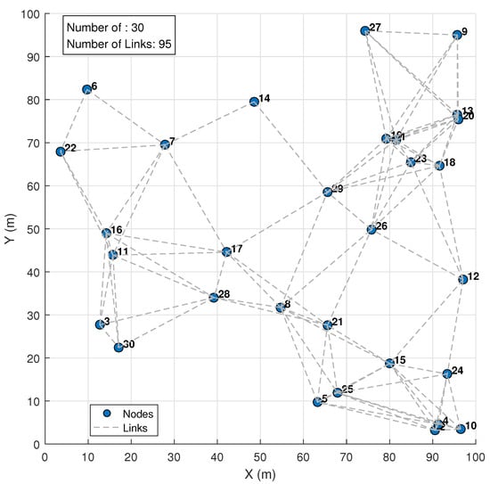
Figure 1. The wireless sensor network scenario for the experiment.

In the OPNET platform, the primary objective was to evaluate network throughput and average energy consumption. OPNET is a powerful discrete-event network simulator renowned for its high-fidelity modeling of communication protocols and network traffic. To leverage its strengths in simulating network dynamics and data flow, a scenario with 20 nodes was configured. This scale is computationally efficient for OPNET’s detailed protocol stack emulation while being sufficiently complex to generate meaningful data on how link scheduling strategy impact aggregate throughput and the rate of energy dissipation across the network.

In the OpenET platform, the experiments were designed to measure the network lifetime. OpenET is a specialized toolkit for simulating energy consumption in WSNs. To effectively stress-test the network’s longevity, the simulation was set up with a network of 50 sensor nodes randomly deployed within a 100 m × 100 m monitoring area. This larger scale increases the multi-hop relay burden and accelerates energy depletion, particularly for nodes near the sink, thereby providing a clear and accelerated view of the network’s energy sustainability and allowing for a robust comparison of strategies aimed at prolonging the operational lifetime. The key parameters for the energy model were defined as follows: the initial energy for each sensor node was set to 0.5 Joules, the transmitter and receiver electronics energy consumption was 50 nJ/bit, and the transmit amplifier energy was set to 100 pJ/bit/m² for the free-space model. The simulation was run for a maximum of 2000 rounds or until the all nodes depletes its energy.

5.3. Comparison of Algorithms

A comparative analysis of the TSO-LS, GA, PSO, EPSO, and ACO algorithms is presented in Figure 2 and Table 3, which illustrates their respective performance in terms of energy efficiency, latency, and overall comprehensive performance.The results show that TSO-LS improves energy efficiency by 13.3% over the GA algorithm, and a 12.5% reduction in average latency. Under different experimental conditions, the TSO-LS strategy shortens the average latency to 10.5 ms. Compared with the GA algorithm, the overall algorithm score of TSO-LS increased from 0.879 to 1.0. TSO-LS demonstrates a clear advantage in key evaluation metrics such as energy efficiency and average delay.

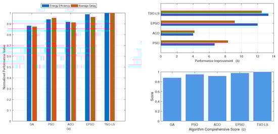
Figure 2. Experimental Performance of Multi-Metric Link Scheduling. (a) Normalized Energy Efficiency and Average Delay; (b) Enhanced Performance Compared to GA; (c) Comprehensive Performance Score.

Table 3. Evaluation Results of MATLAB Experiments.

	GA	PSO	ACO	EPSO	TSO-LS
Energy Efficiency	0.75	0.80	0.78	0.84	0.85
Average Delay	12 ms	11 ms	11.5 ms	10.9 ms	10.5 ms

Note: Bold values indicate the best performance among the compared algorithms.

We simulated the WSN using OPNET to evaluate the performance of different scheduling strategies. Key metrics, including network throughput and energy consumption, are presented in Table 4. The links activated by TSO-LS tend to favor short-range connections, reducing the average energy consumption to 0.32 mJ—a 22% decrease compared to GA. Meanwhile, TSO-LS maintains a high throughput of 5.5 Mbps through dynamic adjustments, validating the effectiveness of the model.

Table 4. Comparative Analysis of OPNET Simulation Results.

	Throughput (Mbps)	Average Energy Consumption (mJ)
ACO	5.2	0.36
EPSO	5.4	0.32
TSO-LS	5.5	0.32
PSO	5.3	0.34
GA	5.1	0.41

Note: Bold values indicate the best performance in each metric.

In WSN studies, the number of rounds is commonly used as a proxy for network lifetime. Within the OpenET platform, the number of rounds required to deplete the operational capacity of all sensor nodes was tested. The results are shown in Figure 3. The TSO-LS algorithm survived for 1180 rounds, demonstrating a 20.4% improvement over GA which survived for 980 rounds.

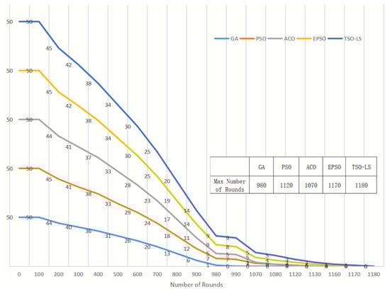
Figure 3. Network Lifetime of Algorithms.

The superior performance of the TSO-LS algorithm in solving the problem of wireless link scheduling strategies, as demonstrated in Figure 2, can be attributed to its unique search mechanisms and the specific improvements tailored for this problem, which effectively address the limitations of GA, PSO, EPSO, and ACO. The results in Figure 2 were obtained through a rigorous simulation under consistent network parameters and performance metrics, with the following key reasons for TSO-LS’s outperformance:

(1) Optimization of the individual Update Mechanism (OUM). As shown in Figure 4, the TS0-LS update mechanism we designed demonstrates significant advantages in the dynamic adjustment of coefficient ${\alpha }_1$ compared to the original version of TSA. The proposed coefficient ${\alpha }_1$ exhibits a noticeably more gradual increase during the initial iteration phase. This intentionally designed gradual increase enables the algorithm to maintain strong exploration capability in early stages while progressively enhancing its exploitation capability as iterations advance. Such effective balance between exploration and exploitation successfully facilitates rapid convergence, thereby achieving the desired optimization efficiency. Unlike PSO, which can prematurely converge due to its strong social component, or GA, whose crossover and mutation are less guided in complex search spaces, the dual-mode search more efficiently navigates the high-dimensional, non-linear solution space of link scheduling.

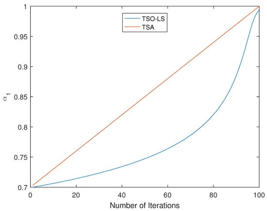
Figure 4. Variation trend of ${\alpha }_1$.

(2) Enhancement of Leading Individual Selection Strategy (ESS). The proposed TSO-LS introduced targeted enhancements—such as the adaptive weight factor for accelerated convergence and the distance-weighted leader selection for better guidance—that are directly aligned with the objectives of minimizing interference and maximizing concurrent transmissions in link scheduling. In contrast, GA, PSO, EPSO and ACO lack such customized mechanisms for this specific domain.

(3) Population Diversity Maintenance (PDM).The optimized individual update mechanism of TSO-LS to converge more rapidly towards high-quality solutions without significant oscillations, a common issue in PSO, or the slower generational progress typical of GA.

As shown in Table 5, the comparison among TSA, TSA + OUM, TSA + ESS, TSA + PDM and TSO-LS demonstrates that OUM achieves the best performance in reducing the number of iterations, while ESS contributes to finding optimal solutions. In contrast, the comprehensively improved algorithm TSA-LS identifies higher-quality solutions with fewer iterations.

Table 5. Comparison of TSA-based algorithms.

	Iterations to Convergence	Final Fitness Value
TSA	154	0.918
TSA + OUM	110	0.939
TSA + ESS	128	0.942
TSA + PDM	156	0.945
TSO-LS	98	0.951

6. Conclusions

This paper addressed the critical and NP-hard problem of efficient link scheduling in resource-constrained WSNs by proposing a novel strategy TSO-LS algorithm. The inherent search mechanisms of the tuna swarm algorithm were integrated with the specific characteristics of the link scheduling problem, and additional algorithmic improvements were introduced to better address the requirements of this scenario.

Experimental evaluations demonstrated the superior performance of the TSO-LS algorithm compared to traditional metaheuristics such as GA, PSO, EPSO, and ACO. Specifically, TSO-LS achieved a remarkable 13.3% improvement in energy efficiency and a 12.5% reduction in average latency. Under various experimental conditions, the TSO-LS strategy consistently shortened the average latency to 10.5 ms. Furthermore, this approach significantly enhanced network energy utilization, reducing the mean node energy consumption from 0.41 mJ to 0.32 mJ, representing an approximate 22% reduction, thereby substantially extending the network’s operational lifespan.Our network lifetime has been extended by 20.4%.

In conclusion, the proposed TSO-LS algorithm offers a robust and effective solution for optimizing link scheduling in WSNs, demonstrating outstanding overall performance in terms of energy efficiency and latency reduction. This work contributes to the development of more sustainable and high-performance WSN deployments. Future research will focus on extending TSO-LS to dynamic network topologies and multi-objective optimization scenarios with more complex constraints.

Limitations and Future Work

While the proposed TSO-LS algorithm demonstrates significant performance in static network environments, its efficacy in highly dynamic scenarios with frequent topological changes remains unverified. Future work will focus on enhancing TSO-LS to handle node mobility and scalability, extend its multi-objective optimization capability to incorporate metrics like throughput and fairness, and explore hybridization with machine learning techniques for adaptive parameter tuning in dynamic networks.

References

- Masood, A. Survey on Energy-Efficient Techniques for Wireless Sensor Networks. arXiv 2021, arXiv:2105.10413. [Google Scholar] [CrossRef]
- Houssein, E.H.; Saad, M.R.; Djenouri, Y.; Hu, G.; Ali, A.A.; Shaban, H. Metaheuristic algorithms and their applications in wireless sensor networks: Review, open issues, and challenges. Clust. Comput. 2024, 27, 13643–13673. [Google Scholar] [CrossRef]
- Yuan, Y.; Zhuo, X.; Liu, M.; Wei, Y.; Qu, F. A centralized cross-layer protocol for joint power control, link scheduling, and routing in UWSNs. IEEE Internet Things J. 2023, 11, 12823–12833. [Google Scholar] [CrossRef]
- Okdem, S.; Karaboga, D. Routing in wireless sensor networks using an ACO router chip. Sensors 2009, 9, 909–921. [Google Scholar] [CrossRef] [PubMed]
- Kumar, P.; Amgoth, T.; Annavarapu, C.S.R. ACO-based mobile sink path determination for wireless sensor networks under non-uniform data constraints. Appl. Soft Comput. 2018, 69, 528–540. [Google Scholar]
- Sharmin, A.; Anwar, F.; Motakabber, S.M.A.; Hashim, A.H.A. Secure ACO-Based Wireless Sensor Network Routing Algorithm for IoT. In Proceedings of the 2021 8th International Conference on Computer and Communication Engineering (ICCCE), Kuala Lumpur, Malaysia, 22–23 June 2021; pp. 190–195. [Google Scholar]
- Kulkarni, R.V.; Venayagamoorthy, G.K. Particle swarm optimization in wireless-sensor networks: A brief survey. IEEE Trans. Syst. Man, Cybern. Part C (Appl. Rev.) 2010, 41, 262–267. [Google Scholar] [CrossRef]
- Tripathy, P.; Khilar, P.M. PSO based Amorphous algorithm to reduce localization error in Wireless Sensor Network. Pervasive Mob. Comput. 2024, 100, 101890. [Google Scholar] [CrossRef]
- Azharuddin, M.; Jana, P.K. Particle swarm optimization for maximizing lifetime of wireless sensor networks. Comput. Electr. Eng. 2016, 51, 26–42. [Google Scholar] [CrossRef]
- Tossa, F.; Abdou, W.; Ezin, E.C.; Gouton, P. Improving coverage area in sensor deployment using genetic algorithm. In Computational Science—ICCS 2020; Springer International Publishing: Cham, Switzerland, 2020; pp. 398–408. [Google Scholar]
- Shahi, B.; Dahal, S.; Mishra, A.; Kumar, S.V.; Kumar, C.P. A review over genetic algorithm and application of wireless network systems. Procedia Comput. Sci. 2016, 78, 431–438. [Google Scholar] [CrossRef]
- Hao, Z.; Hou, J.; Dang, J.; Dang, X.; Qu, N. Game algorithm based on link quality: Wireless sensor network routing game algorithm based on link quality. Int. J. Distrib. Sens. Netw. 2021, 17, 1550147721996248. [Google Scholar] [CrossRef]
- Mohammadi, N.; Bigham, B.S.; Kadivar, M. PDSLS: An approximation SINR-based Shortest Link Scheduling algorithm with power control. Comput. Commun. 2025, 236, 108137. [Google Scholar] [CrossRef]
- Zeng, B.; Liang, Z.; Zhao, C. Sinr-based slot reuse algorithm for multi-channel wireless sensor networks. EURASIP J. Wirel. Commun. Netw. 2025, 2025, 48. [Google Scholar] [CrossRef]
- Tian, H. Enhancing the effectiveness of wireless sensor networks through consensus estimation and universal coverage. Sci. Rep. 2025, 15, 24930. [Google Scholar] [CrossRef]
- Butt, F.A.; Jalil, M.; Liaquat, S.; Alawsh, S.A.; Naqvi, I.H.; Mahyuddin, N.M.; Muqaibel, A.H. Self-calibration of wireless sensor networks using adaptive filtering techniques. Results Eng. 2025, 25, 103775. [Google Scholar] [CrossRef]
- Kamel, S.; Al Qahtani, A.; Al-Shahrani, A.S.M. Particle Swarm Optimization for Wireless Sensor Network Lifespan Maximization. Eng. Technol. Appl. Sci. Res. 2024, 14, 13665–13670. [Google Scholar] [CrossRef]
- Wang, L.; Xiao, Y. A survey of energy-efficient scheduling mechanisms in sensor networks. Mob. Netw. Appl. 2006, 11, 723–740. [Google Scholar] [CrossRef]
- Xie, L.; Han, T.; Zhou, H.; Zhang, Z.R.; Han, B.; Tang, A. Tuna swarm optimization: A novel swarm-based metaheuristic algorithm for global optimization. Comput. Intell. Neurosci. 2021, 2021, 9210050. [Google Scholar] [CrossRef] [PubMed]
- Tang, J.; Liu, G.; Pan, Q. A review on representative swarm intelligence algorithms for solving optimization problems: Applications and trends. IEEE/CAA J. Autom. Sin. 2021, 8, 1627–1643. [Google Scholar] [CrossRef]
- Tan, M.; Li, Y.; Ding, D.; Zhou, R.; Huang, C. An improved jade hybridizing with tuna swarm optimization for numerical optimization problems. Math. Probl. Eng. 2022, 2022, 7726548. [Google Scholar] [CrossRef]
- Xiao, X.; Tan, G.; Gao, C.; Tang, X.; Song, W.; Tian, Y. A Multi-Strategy Improved Tuna Swarm Optimization Algorithm for Cloud Task Scheduling. In Proceedings of the 2024 5th International Symposium on Computer Engineering and Intelligent Communications (ISCEIC), Wuhan, China, 8–10 November 2024; pp. 174–179. [Google Scholar]
- Wang, W.; Tian, J. An improved nonlinear tuna swarm optimization algorithm based on circle chaos map and levy flight operator. Electronics 2022, 11, 3678. [Google Scholar] [CrossRef]
- Srinivasan, B.; Kalimuthu, V.K.; Muthu, T.; Velumani, R. Modeling of tuna swarm algorithm based unequal clustering approach on internet of things assisted networks. Braz. Arch. Biol. Technol. 2024, 67, e24231115. [Google Scholar] [CrossRef]
- Daneshvar, S.M.M.H.; Mazinani, S.M. On the best fitness function for the WSN lifetime maximization: A solution based on a modified salp swarm algorithm for centralized clustering and routing. IEEE Trans. Netw. Serv. Manag. 2023, 20, 4244–4254. [Google Scholar] [CrossRef]
- Kapoor, R.; Sharma, S. Hybrid metaheuristic optimization for energy-efficient routing, clustering, and sleep scheduling in WSNs. In Wireless Ad-Hoc and Sensor Networks; CRC Press: Boca Raton, FL, USA, 2024; pp. 156–176. [Google Scholar]
- Yuan, J.; Peng, J.; Yan, Q.; He, G.; Xiang, H.; Liu, Z. Deep reinforcement learning-based energy consumption optimization for Peer-to-Peer (P2P) communication in wireless sensor networks. Sensors 2024, 24, 1632. [Google Scholar] [CrossRef]
- Jerbi, W.; Cheikhrouhou, O.; Guermazi, A.; Trabelsi, H. An enhanced MSU-TSCH scheduling algorithms for industrial wireless sensor networks. Concurr. Comput. Pract. Exp. 2024, 36, e7938. [Google Scholar] [CrossRef]
- Khiar, A.; Mazouzi, S.; Benaboud, R.; Haouassi, H. Binary Tuna Swarm Optimization Algorithm-Based Feature Selection for Intrusion Detection Systems. J. Commun. Softw. Syst. 2025, 21, 383–393. [Google Scholar] [CrossRef]
- Wang, X.; Liu, Y.; Xue, G.; Bai, F.; Huang, S. Fast Non-Dominated Sorting Tuna Swarm Optimization Algorithm (FNS-TSO): Time-Energy-Impact Multi-Objective Optimization of Underwater Manipulator Trajectories. J. Mar. Sci. Eng. 2025, 13, 916. [Google Scholar] [CrossRef]
- Periasamy, J.K.; Mallick, S.; Chitti, S.; Sivasakthi, S.; Kv, B.; Puliyanjalil, E. Tuna Swarm Algorithm Based Robust Node Localization Scheme in Wireless Communication Networks. Int. Res. J. Multidiscip. Scope 2025, 6, 1426–1437. [Google Scholar] [CrossRef]
- Kannan, S.K.; Diwekar, U. An enhanced particle swarm optimization (PSO) algorithm employing quasi-random numbers. Algorithms 2024, 17, 195. [Google Scholar] [CrossRef]
Disclaimer/Publisher’s Note: The statements, opinions and data contained in all publications are solely those of the individual author(s) and contributor(s) and not of MDPI and/or the editor(s). MDPI and/or the editor(s) disclaim responsibility for any injury to people or property resulting from any ideas, methods, instructions or products referred to in the content. |
© 2025 by the authors. Licensee MDPI, Basel, Switzerland. This article is an open access article distributed under the terms and conditions of the Creative Commons Attribution (CC BY) license (https://creativecommons.org/licenses/by/4.0/).