Addressing Daigou from the Perspective of Channel Competition: Strategy for Retail Management

Abstract

In China’s on-demand service platforms, daigou agents utilize locational differences through proxy purchasing. Daigou creates an informal supply chain that directly competes with official channels. This study incorporates daigou arbitrage into the channel competition framework via a multi-stage Stackelberg game-theoretic model. An analysis of the subgame perfect Nash equilibrium shows that daigou activity disrupts the manufacturer’s profits. We have thus developed a strategy based on mathematical optimization and compared its effectiveness and side effects with those of existing methods. We came to identify purchase restrictions as one of the most powerful strategies. Equilibrium analysis and numerical experiments confirm that proper purchase restriction choices reduce daigou arbitrage and minimize negative impacts on legitimate demand. This work provides the first game-theoretic model that integrates informal proxy-purchase supply chains into dual-channel competitions.

1. Introduction

Daigou is derived from the Chinese term for “purchasing on behalf”. Daigou activities involve individuals or networks acting as intermediaries to acquire and resell goods. It often involves price markup through informal channels such as social media platforms or e-commerce apps. The daigou phenomenon originated in cross-border contexts. As Chinese consumers sought overseas luxury goods and pharmaceuticals due to tariffs, quality concerns, and price advantages, daigou has become a billion-dollar informal economy [1]. In recent years, resellers in China have benefited from localized supply constraints and viral demand for premium regional products. This shift is further accelerated by digital mobile applications. They enable real-time inventory sharing and livestreaming sales, increasing competition with formal retail channels by creating parallel distribution networks that affect pricing control and supply chain predictability [2,3].

The rise of daigou (also known as “proxy shopping”) in China shows a transformation of retail and consumer behavior, driven by fragmented supply chains, domestic demand asymmetries, and the growth of digital platforms. Initially, daigou was primarily associated with cross-border e-commerce driven by factors such as exchange rate differences and tax advantages. However, it has since become a domestic phenomenon, particularly in urban retail, where consumers increasingly rely on intermediaries to access high-demand goods from niche or regionally concentrated suppliers. This practice has created digital platform-based labor networks, redefining the boundaries between traditional retail, non-traditional work arrangements, and consumer-driven market dynamics. For example, Pang Donglai (www.azpdi.cn), a regional supermarket chain in China renowned for its premium service with a limited physical expansion, served as a notable example of how cross-border daigou activity has shifted to the domestic market. Although Pang Donglai currently operates in only two cities within Henan Province, China, its reputation for high product quality and customer experiences has gained significant demands from other places outside Henan Province. However, Pang Donglai provides no online shopping and delivery services to its customers. Thus, when customers want to buy Pang Donglai’s high-quality products, they have to shop at their physical stores. Quite often, Pang Donglai customers have to queue outside these stores before they can shop. Customers from outside Henan Province must endure long travel times just to reach Pang Donglai stores, while even those from nearby regions often face hours of queuing before they can shop. To provide convenient and time-saving services to these Pang Donglai customers, domestic daigou agents emerged, who would collect orders from customers living in local regions or outside Henan Province, queue up outside Pang Donglai’s stores, and purchase the items for their customers. The orders are completed by shipping these products to the customers via delivery networks. Many leading professional daigou operators would set up physical bases near Pang Donglai stores to complete their daigou activities in a more efficient way. However, the large volume of these daigou customers has overwhelmed Pang Donglai’s operational capacity and compromised its service standards. To tackle these problems, Pang Donglai has implemented targeted interventions, including purchase restrictions on high-demand items to reduce the chances of product shortage. The conflicts between institutionalized retail models and platform-driven consumption practices reveal the need for a systematic analysis of daigou activities to understand the implications for supply chain resilience, labor organization, and evolving consumer behavior.

From a channel competition perspective, daigou represents a disruptive force in the retail ecosystem. Informal intermediaries compete with formal channels for consumer access and brand loyalty. In China, this is reflected in resellers benefiting from arbitrage opportunities such as regional exclusivity or promotional pricing. Daigou resells goods at a premium for convenience and accessibility, which results in the substitution effects that disrupt existing sales offers and reduces brand control. For instance, cross-border daigou for luxury brands often involves lower prices than domestic prices through tax avoidance, accounting for over 20% of China sales in some categories [2]. However, domestic iterations extend this competition to retail. This is reflected in large-scale retailers like Pang Donglai facing bulk-purchase resellers who charge markups to distant consumers. This increases the pressure on store operations and thus requires managerial intervention to safeguard service quality and supply chain resilience.

The case of Pang Donglai shows how domestic daigou can disrupt institutionalized retail models by creating unanticipated demand pressures and operational challenges. The existing literature has focused on cross-border daigou such as luxury goods and pharmaceuticals. Scalper-driven daigou operations often focus on limited-production products. However, the domestic daigou remains underexplored in standard retail settings. For example, studies often consider daigou as a cross-border phenomenon involving overseas procurement for mainland Chinese consumers, such as in Hong Kong or Western markets. The daigou serves as a “middleman” connecting customers to global brands through informal networks [3]. Prior research has extensively examined cross-border daigou in luxury goods and scalping in limited-edition products, but few studies have addressed its domestic iterations in standard retail settings. Therefore, the literature limits the understanding of how daigou influences channel integration, supply chain agility, and competitive strategies in fragmented markets [4]. Thus, it raises questions about how domestic daigou operates within retail ecosystems, its implications for supply chain resilience and consumer behavior, and the policy responses needed to address its challenges. Recent research also point out that daigou is still largely “under-researched” as an unconventional entrepreneurial setup, especially in non-luxury retail markets [5]. Hence, these questions show a gap in the literature, which this study tries to address.

To address these gaps, this study examines domestic daigou from the perspective of channel competition through a comparison between a base model without daigou, a model incorporating daigou, and a model with daigou under constraints. This comparative analysis explores the following research questions:

• RQ1: How does the presence of daigou affect retail channel conflicts compared to scenarios without daigou?
• RQ2: What are the impacts of constraints like purchase limits on daigou dynamics and retailer strategies for management and resilience?
• RQ3: How do asymmetric substitution effects between daigou and official channels influence equilibrium outcomes and competition in the models?

From the analysis of theoretical models of multi-channel competition, this research contributes a framework for retail managers to navigate daigou dynamics, offering actionable strategies to reclaim channel control.

2. Literature Review

Daigou is defined as a practice that combines operations management, digital commerce, and economic theory by purchasing goods and reselling them at higher prices. The daigou agents act as speculators, taking advantage of price differences rather than making direct sales. On the other hand, daigou also shares some similarities with the on-demand service platforms. In this case, independent agents serve as intermediaries who respond to individual consumer requests, sourcing goods or services and exploiting price or availability differences. However, few analyses have applied quantitative frameworks to capture daigou’s distinct setup. To fill this gap, our work proposes a Stackelberg leader–follower strategic model. In this model, the manufacturer sets rules to increase market efficiency and consumer benefit, while the daigou adjusts both price and volume decisions under these constraints.

2.1. Speculative Selling and Scalping

In terms of speculative selling, systematic research on this dates back to the 1970s, when academics began studying how inventories are transferred across periods from an arbitrage perspective. Rather than depending on general intuition, Kohn [6] employed a rigorous structure to illustrate how the cost of carrying and changing market prices drive stock adjustments in commodities, thereby focusing attention on real rather than rational behavior. Drawing on these studies, Tirole [7] questioned the results of the former study and instead explained persistent profits through a heterogeneity of beliefs across traders. While these models provide utility, they often struggle to accommodate barriers encountered in a real-life transaction environment. Ticket scalping is a good example of speculative behavior in the market. Scalpers purchase tickets at lower prices, then sell at higher prices as the ticket date approaches, taking advantage of on-demand fluctuations and temporal price variations [8,9,10].

More recent research expands the definition of speculative selling to include both speculators and forward-looking customers [11,12,13,14]. The study [11] proposes an equilibrium where the manufacturer limits initial availability. The manufacturer can increase profit through willing-to-wait consumers while reducing the volume of speculative purchases at the same time. The study [14] shows that dynamic pricing mechanisms can also increase profit by adjusting prices in response to inventory risk and market demand fluctuations. On the other hand, ref. [15] further develops this direction and demonstrates how manufacturers can observe the uncertainties of market speculation while effectively managing consumer purchasing timing. These approaches, in the end, allow manufacturers to increase their profits even when facing limited resources and unpredictable consumer behavior. However, these models assume symmetric profit maximization and regulated markets. For the gray markets, they exploit the price differences, regulatory gaps, and cost asymmetries that disrupt the conventional supply chain. Therefore, this shows the importance of adjusting these models to include daigou contexts.

2.2. Cross-Border Daigou and Gray Markets

Cross-border daigou takes advantage of price differences between countries or regions. Daigou agents purchase from markets with lower prices, then sell in markets with higher prices. This approach adds a spatial factor to gray market corss-border arbitrage. There is extensive descriptive research on investigating cross-border daigou practices. Some studies show that cross-border daigou sellers choose product categories where pricing differences are large; this includes cosmetics, infant formula, and also luxury items [1,16,17]. The work [3] investigates the bodily motions that facilitate the flow of people between Mainland China and Hong Kong. It also shows how physical travel, combined with digital platforms, creates labor hierarchies and power asymmetries. Bai [18] suggests that luxury brands often struggle with controlling their widespread businesses, which can often bypass official supply chains. Recent work [5] frame daigou participants as entrepreneurial intermediaries, which allow them to fill market gaps that formal supply chains leave open.

Recent mathematical models consider daigou-driven arbitrage as a strategic game. Game-theoretic models suggest that manufacturers can oppose parallel imports, like daigou actors, by changing how they distribute products, lowering product quality, or timing market entrance based on regional differences in how many consumers are willing to purchase [19]. Another analytical model in [20] suggests that allowing restricted gray market activity could potentially increase total profits. This matches when luxury markets are large and the costs of international transactions are relatively low. A recent empirical study of informal secondary markets support this idea. Prasetyo [21] investigated how digital platforms operate in informal economies. The study showed how social networks help to promote gray market activities in reselling.

2.3. Domestic Daigou and Sharing Economy

Cross-border daigou focuses on price differences and global supply chain challenges. However, a unique practice has developed in domestic and regional markets. This practice is closely related to the sharing economy principles. Platforms like errand-running services (paotui, meaning “running legs” in Chinese) and on-demand delivery networks support that identity develops through access, not ownership [22]. They emphasize spatial proximity and real-time responsiveness instead of the price differences between countries or regions. So, the domestic models in fact differ from cross-border daigou, that is, the domestic models emphasize time-sensitive transactions. This includes acquiring limited-edition items, addressing domestic supply chain issues, and meeting hyperlocal consumer demands. This shows how the sharing economy aims to increase access to underused resources. As a result, digital platforms play a key role by improving trust and efficiency in these domestic operations [23,24].

The recent growth of these platforms is supported by mobile technologies, real-time data analytics, and matching systems. These tools provide effective coordination between consumers and micro-entrepreneurs or freelancers [25,26,27]. Research uses game-theoretic and queuing-theoretic frameworks to analyze the interplay between supply and demand. For example, Stackelberg hierarchies represent platforms as leaders that create surge pricing [28] and commissions [29]. On the other hand, Hotelling models analyze competition in multi-homing applications [30]. Queuing-theoretic approaches [27,31,32] analyze decisions on pricing, wages, and staffing under uncertainty. Reputation systems [33] help minimize matching issues to improve the system performance. A recent study [34] on informal markets in the sharing economy explored dual-channel supply chain competition during pandemic-induced demand disruptions. The authors discuss how informal reselling changes to platform-mediated constraints in e-commerce.

2.4. Dual-Channel Competition and Omni-Channel Retailing

Research on dual-channel competition and omni-channel retailing provides a deeper understanding of how daigou disrupts traditional supply chains. Recent studies on omni-channel retail demonstrated the importance of platform-mediated channels and informal markets in modern e-commerce. The work [35] examined omni-channel retailing technologies through a systematic review. It showed that integrating online and offline channels can reduce informal reselling by directing demand to formal platforms. The work [36] examined the challenges of retail in omni-channel. It also developed a scale to identify omni-channel obstacles, showing that digital tools can reduce the reliance on informal intermediaries such as daigou. Also, the work [37] proposed a systematic review and a future research for omni-channel management in the modern retailing setup. It emphasized the need to integrate informal channels into formal strategies to improve the resilience of the supply chain.

In this research, we focus on the manufacturer-centric control in the presence of domestic daigou. We develop a Stackelberg leader–follower game structure. The manufacturer acts as the leader, and the domestic daigou agent acts as the follower. This approach is different from the prior platform-centric models through pricing and commission strategies [28]. Instead, we focus on the manufacturer strategy that can influence the domestic daigou behavior. Then, we optimize the supply chain efficiency, pricing, and profits. Our analysis explores a novel manufacturer strategy with purchasing limitation. This strategy is closely related to the regulatory effects imposed by China’s E-Commerce Law, which adds purchase restrictions via mandatory registration and taxation [38]. However, our approach achieves a similar outcome by limiting arbitrage, likely by redirecting the demand back to the official channels through supply chain mechanisms rather than policy interventions.

3. The Model

In this study, we analyze a supply chain with a single manufacturer and a single domestic daigou. We also focus on a single product to isolate the strategic interactions within this market structure. As empirical motivations often emphasize the networks of daigou agents and retailers, our choice of a single daigou agent simplifies the model to focus solely on the strategy. This is common in the supply chain literature for analytical tractability [39]. Hence, it allows us to derive closed-form expressions in pricing and demand, though future extensions could incorporate multiple agents to capture competition among daigou. On the other hand, we consider that the manufacturer also operates as a retailer, offering the product directly to consumers through traditional sales channels. Then, the domestic daigou enters the market by sourcing the same product from the manufacturer and reselling it. The domestic daigou prioritizes the convenience of remote purchasing and “proxy shopping”.

We develop three models to capture different market dynamics, and the three models are shown below in Figure 1:

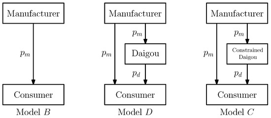
Figure 1. Direct Channel Model, Daigou Entry Model and Constrained Daigou Model.

• Direct Channel Model (B): The manufacturer acts as the sole retailer, selling directly to consumers. This model is a benchmark for evaluating the impact of introducing a domestic daigou. It focuses on optimal pricing and demand in a simple direct channel setting.
• Daigou Entry Model (D): When a domestic daigou is introduced, the product is sourced from the manufacturer at the retail price and is resold to convenience-seeking consumers. This model focuses on the impact of domestic daigou entry on pricing and demand, as well as the profits.
• Constrained Daigou Model (C): Building on the Daigou Entry Model, we introduce a constraint on the purchase quantity for the daigou. This extends the Daigou Entry Model and analyzes how purchase constraint affects strategic decisions and channel efficiency.

The primary objective of this research is to analyze the pricing, demand, and overall profitability within a single-manufacturer single-domestic daigou supply chain. We developed and analyzed three sequential models for the Stackelberg game for analysis. The baseline is the Direct Channel Model. We then introduce the domestic daigou in the Daigou Entry Model, and find the impact of the presence of this intermediary. Based on the Daigou Entry Model, the Constrained Daigou Model introduces a purchase limit on the domestic daigou, allowing us to analyze how such purchase constraints affect the decisions and channel efficiency.

In this study, we use the following notation to describe the key variables and parameters. The manufacturer’s sales price is denoted by $p_m$, while the daigou’s sales price is denoted by $p_d$. In Models D and C, the parameters ${\theta }_d$ and ${\theta }_m$ are the asymmetric channel substitution parameters, where ${\theta }_d$ and ${\theta }_m$ represent the degree of substitution from the domestic daigou to the manufacturer and from the manufacturer to the domestic daigou, respectively. The superscripts $\{B,D,C\}$ are used to distinguish the models. In Models D and C, they incorporate the asymmetric channel substitution effects. Therefore, they capture the competitive dynamics between the formal manufacturer’s direct channel and informal daigou channels. From the channel competition and differentiation [40,41,42], these parameters (${\theta }_m^D$ and ${\theta }_d^D$) represent the degrees of substitutability between the two channels, where ${\theta }_m^D,{\theta }_d^D\in (0,1)$. Lower values of these parameters indicate weaker substitution; higher values represent near-perfect substitutability.

We assume ${\theta }_d^D>{\theta }_m^D$; this means the domestic daigou has a greater substitutive impact on the manufacturer’s direct channel demand. Theoretically, this asymmetry arises from the daigou’s provision of differentiated value-added services that the manufacturer’s direct channel often cannot copy. These services attract consumers who might initially consider the direct channel but switch to the daigou for convenience [43,44]. On the other hand, the manufacturer’s direct channel typically does not match the daigou’s service level. Therefore, it is less likely to draw away the daigou’s consumers.

We assume the manufacturer’s marginal production cost is constant at c, with $c\in (0,a)$, where a represents the market size. For the domestic daigou in Models D and C, the procurement cost equals the manufacturer’s direct-channel retail price, $c_d^D=p_m^D$, as daigou operate as unauthorized, informal resellers who source products at standard retail prices from official websites or stores, without access to wholesale agreements, minimum-order quantity waivers, volume discounts, or tiered pricing [16,44,45]. This retail price procurement is a feature of retail-level gray markets and daigou channels, where intermediaries effectively act as high-volume consumers rather than contracted distributors. Manufacturers can employ discriminatory or wholesale pricing to deter arbitrage by authorized distributors, such strategies are ineffective against informal daigou, who source covertly or through consumer-facing retail channels. This assumption therefore reflects actual daigou practices in China-dominated markets and is standard in gray-market models of unauthorized parallel importation. Additional operational costs are omitted for analytical tractability, following the common practice detailed in the dual-channel literature [46,47].

We denote e as the level of value-adding effort deployed by the domestic daigou, which may include personalized marketing, faster local delivery, etc. Accordingly, $\gamma >0$ represents the marginal effectiveness of this effort in expanding primary demand. The expanded market potential available to the daigou channel is thus modeled as $a+\gamma e$, where a represents the original market size reachable via the manufacturer’s direct channel alone, and the incremental term $\gamma e>0$ captures the daigou’s role in stimulating new primary demand among previously time-sensitive or convenience-seeking consumers, following established models of channel expansion and effort-driven demand growth [48,49,50,51].

Building on these channel dynamics, in modeling the daigou’s effort e in Model D and Model C, we assume it expands demand linearly via parameter $\gamma$, as this captures constant marginal returns to effort in stimulating consumer interest and simplifies the demand function for tractability [52] to represent realistic advertising for market share. The costs are quadratic, parameterized by $\eta$, to reflect increasing marginal costs, diminishing returns, and convexity, ensuring the profit function is concave for unique equilibria. This is a structure commonly used in marketing and supply chain models [48,53]. This relationship is empirically substantiated by studies on intermediary efforts in e-commerce and proxy markets, where increased personalization, marketing, and service efforts correlate with demand growth but require ongoing investments that can escalate with scale. For instance, qualitative interviews with 27 daigou practitioners highlighted how efforts like physical sourcing trips build trust and facilitate demand in cross-border commodity chains [3].

The game sequences in all three models follow a consistent decision sequence: the manufacturer first determines the price, and the domestic daigou then sets the selling prices for the product based on the observed strategy from the manufacturer.

• In Model B, the manufacturer sets the direct sales price $p_m^B$, and there is no domestic daigou in this model.
• In Model D, the manufacturer first sets the direct sales price $p_m^D$, after which the domestic daigou purchases at this price and sets the retail price $p_d^D$, where $p_d^D>p_m^D$.
• In Model C, the manufacturer first sets the direct sales price $p_m^C$ and the purchase quantity limit $Q^C$ for the consumers. Then, the domestic daigou purchases at the price $p_m^C$ and sets the retail price $p_d^C$, where $p_d^C>p_m^C$.

The steps outlined above are also illustrated in the visual summary of the game sequence in Figure 2.

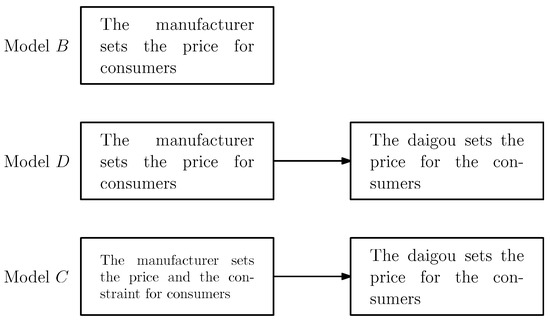
Figure 2. Game sequences of the models.

The notations used in this paper are summarized in Table 1.

Table 1. Summary of notations.

Notation	Explanation
x	$x\in \{m,d\}$, where m and d denote the manufacturer and the daigou, respectively
y	$y\in \{B,D,C\}$, where B, D, and C denote the base model, daigou model, and constrained daigou model, respectively
${\theta }_x^y$	The substitution effect of x in y
a	The market size
c	The unit cost of the product
$p_x^y$	The retail price of x in y
$q_x^y$	The quantity of x in y
$e_x^y$	The daigou’s effort level of x in y
$\gamma$	The influence of efforts on demand
$\eta$	The parameter of the market cost
${\mathsf{\Pi }}_x^y$	The profit of x in Mode y
$Q^C$	The constraint of the daigou’s purchase quantity in Model C

3.1. Direct Channel Model

In the Direct Channel Model, the manufacturer operates as the sole retailer in a single-channel market, serving consumers directly without intermediaries. As defined in the general setup, the baseline market size is $a^B=a>0$, which represents the maximum consumer willingness-to-pay in the absence of daigou entry. The manufacturer incurs a constant marginal production cost c, where $0<c<a$, to ensure positive profitability. Let $q_m^B\ge 0$ denote the manufacturer’s equilibrium sales quantity. With standard linear inverse demand functions in supply chain models, the manufacturer’s retail price is determined by

$$\begin{array}{cc}\hfill p_m^B& =a^B-q_m^B\hfill \end{array}$$

(1)

$$\begin{array}{cc}\hfill & =a-q_m^B\hfill \end{array}$$

(2)

So, we have the profit function

$$\begin{array}{c}\hfill {\mathsf{\Pi }}_m^B=(p_m^B-c)q_m^B.\end{array}$$

(3)

Then, we have the following proposition.

Proposition 1.

In the Direct Channel Model, the maximum profit

$$\begin{array}{c}\hfill {\mathsf{\Pi }}_m^{B\ast }={\displaystyle \frac{{(a-c)}^2}{4}},\end{array}$$

(4)

where the optimal sales quantity $q_m^{B\ast }={\displaystyle \frac{a-c}{2}}$ and the optimal sales price $p_m^{B\ast }={\displaystyle \frac{a+c}{2}}$.

Proof. 

See Appendix A. □

3.2. Daigou Entry Model

We extend our baseline Direct Channel Model by incorporating the entry of a domestic daigou, establishing a dual-channel supply chain structure as detailed in the general setup. In this model, the manufacturer and daigou compete as independent retailers serving distinct consumer segments, introducing channel competition that expands market access for consumers facing barriers in the direct channel. This competition is modulated by the asymmetric substitution parameters ${\theta }_d^D>{\theta }_m^D$, where the daigou’s stronger pull ${\theta }_d^D$ reflects its value-added services, potentially cannibalizing the manufacturer’s demand more than vice versa.

Let $q_m^D$ and $q_d^D$ represent the equilibrium quantities supplied by the manufacturer’s direct channel and the daigou, respectively. As per the effort-driven demand expansion in the general model, the daigou’s presence increases the overall market size from the baseline $a^B=a$ to $a^D=a+\gamma e>a^B$, reflecting greater consumer reach through the informal channel [48,49,50,51]. The daigou incurs quadratic costs parameterized by $\eta$ for these efforts, introducing a trade-off that influences its pricing and quantity decisions while ensuring concave profits for equilibrium analysis.

Hence, the inverse demand function is

$$\begin{array}{cc}\hfill p_m^D& =a-{\theta }_d^D{q}_d^D-q_m^D\hfill \end{array}$$

(5)

and

$$\begin{array}{cc}\hfill p_d^D& =a+\gamma e^D-q_d^D-{\theta }_m^D{q}_m^D.\hfill \end{array}$$

(6)

Then, the profit functions are obtained as

$$\begin{array}{cc}\hfill {\mathsf{\Pi }}_m^D& =(p_m^D-c)(q_m^D+q_d^D)\hfill \end{array}$$

(7)

and

$$\begin{array}{cc}\hfill {\mathsf{\Pi }}_d^D& =(p_d^D-c_d^D)q_d^D-{\displaystyle \frac{\eta {\left(e^D\right)}^2}{2}}\hfill \end{array}$$

(8)

$$\begin{array}{cc}\hfill & =(p_d^D-p_m^D)q_d^D-{\displaystyle \frac{\eta {\left(e^D\right)}^2}{2}},\hfill \end{array}$$

(9)

where $\eta$ is the effort cost coefficient.

Proposition 2.

In the Daigou Entry Model, given that ${\displaystyle \frac{{\gamma }^2}{\eta }}<2(1-{\theta }_d^D)$, the maximum profit

$$\begin{array}{c}\hfill {\mathsf{\Pi }}_m^{D\ast }={\displaystyle \frac{(\eta (3-2{\theta }_d^D-{\theta }_m^D)-{\gamma }^2){(a-c)}^2}{4(\eta (2-{\theta }_d^D-{\theta }_d^D{\theta }_m^D)-{\gamma }^2)}},\end{array}$$

(10)

and

$$\begin{array}{c}\hfill {\mathsf{\Pi }}_d^{D\ast }={\displaystyle \frac{\eta (2\eta (1-{\theta }_d^D)-{\gamma }^2){(1-{\theta }_m^D)}^2{(a-c)}^2}{4(\eta (2-{\theta }_d^D-{\theta }_d^D{\theta }_m^D)-{\gamma }^2)}},\end{array}$$

(11)

where the optimal effort is $e^{C\ast }={\displaystyle \frac{\gamma (1-{\theta }_m^D)(a-c)}{2(\eta (2-{\theta }_d^D-{\theta }_d^D{\theta }_m^D)-{\gamma }^2)}}$, the optimal sales quantities are $q_m^{D\ast }={\displaystyle \frac{(2\eta (1-{\theta }_d^D)-{\gamma }^2)(a-c)}{2(\eta (2-{\theta }_d^D-{\theta }_d^D{\theta }_m^D)-{\gamma }^2)}}$ and $q_d^{D\ast }={\displaystyle \frac{\eta (1-{\theta }_m^D)(a-c)}{2(\eta (2-{\theta }_d^D-{\theta }_d^D{\theta }_m^D)-{\gamma }^2)}}$, and the optimal sales prices are $p_m^{D\ast }={\displaystyle \frac{a+c}{2}}$ and $p_d^{D\ast }={\displaystyle \frac{a(\eta (3-2{\theta }_d^D-{\theta }_m^D)-{\gamma }^2)+c(\eta (2-{\theta }_m^D-{\theta }_d^D{\theta }_m^D)-{\gamma }^2)}{2(\eta (2-{\theta }_d^D-{\theta }_d^D{\theta }_m^D)-{\gamma }^2)}}$.

Proof. 

See Appendix A. □

From Proposition 2, we see that the constraint ${\displaystyle \frac{{\gamma }^2}{\eta }}<2(1-{\theta }_d^D)$ is required in the proof of Proposition 2 (see Appendix A). This constraint also guarantees the denominator of ${\mathsf{\Pi }}_m^{D\ast }$ and ${\mathsf{\Pi }}_d^{D\ast }>0$. To show this, let the denominator term in both ${\mathsf{\Pi }}_m^{D\ast }$ and ${\mathsf{\Pi }}_d^{D\ast }$ be $4(\eta (2-{\theta }_d^D-{\theta }_d^D{\theta }_m^D)-{\gamma }^2)$. So, we have

$$\begin{array}{ccccc}\hfill & \hfill & \hfill \eta (2-{\theta }_d^D-{\theta }_d^D{\theta }_m^D)-{\gamma }^2& >0\hfill & \end{array}$$

(12)

$$\begin{array}{cccc}\hfill & \iff \hspace{1em}\hspace{1em}\hspace{1em}\hspace{1em}\hspace{1em}\hspace{1em}\hspace{1em}\hspace{1em}\hfill & \hfill {\theta }_d^D& <{\displaystyle \frac{2}{1+{\theta }_m^D}}\left(1-{\displaystyle \frac{{\gamma }^2}{2\eta }}\right).\hfill \end{array}$$

(13)

Moving the terms from the constraint, we have ${\theta }_d^D<1-{\displaystyle \frac{{\gamma }^2}{2\eta }}$. As ${\theta }_m^D<1$, we have ${\displaystyle \frac{2}{1+{\theta }_m^D}}>1$. Thus, we have

$$\begin{array}{c}\hfill {\theta }_d^D<1-{\displaystyle \frac{{\gamma }^2}{2\eta }}<{\displaystyle \frac{2}{1+{\theta }_m^D}}\left(1-{\displaystyle \frac{{\gamma }^2}{2\eta }}\right).\end{array}$$

(14)

Hence, this constraint implies the profits ${\mathsf{\Pi }}_m^{D\ast }>0$ and ${\mathsf{\Pi }}_d^{D\ast }>0$.

3.3. Constrained Daigou Model

In this section, we examine a constrained variant of the Daigou Entry Model in which the domestic daigou faces a purchase limit $Q^C$ per period. We keep the same parameterization as the Daigou Entry Model and replace the superscript D with C to denote the constrained setting. This limit represents a strategic mechanism that the manufacturer can impose to mitigate service degradation for primary customers by restricting daigou procurement. In practice, such constraints can be implemented through mechanisms like membership cards, which limit purchase quantities within a specified period. We characterize the equilibrium as a function of $Q^C$ and conduct a comparative analysis relative to the unconstrained domestic daigou.

Let $\overline{q_d^C}=min\{q_d^C,Q^C\}$. So, from the inverse functions

$$\begin{array}{cc}\hfill p_m^C& =a-{\theta }_d^C\overline{q_d^C}-q_m^C,\hfill \end{array}$$

(15)

$$\begin{array}{cc}\hfill p_d^C& =a+\gamma e-\overline{q_d^C}-{\theta }_m^C{q}_m^C.\hfill \end{array}$$

(16)

Then, we have the profit functions

$$\begin{array}{cc}\hfill {\mathsf{\Pi }}_m^C& =(p_m^C-c)(q_m^C+\overline{q_d^C})\hfill \end{array}$$

(17)

and

$$\begin{array}{cc}\hfill {\mathsf{\Pi }}_d^C& =(p_d^C-c_d^C)\overline{q_d^C}-{\displaystyle \frac{\eta {\left(e^C\right)}^2}{2}}\hfill \end{array}$$

(18)

Proposition 3.

In the Constrained Daigou Model, if the purchase limit $Q^C<{\displaystyle \frac{\eta (1-{\theta }_m^C)(a-c)}{2(\eta (2-{\theta }_d^C-{\theta }_d^C{\theta }_m^C)-{\gamma }^2)}}$, then the maximum profit

$$\begin{array}{c}\hfill {\mathsf{\Pi }}_m^{C\ast }={\displaystyle \frac{{((a-c)+(1-{\theta }_d^C)Q^C)}^2}{4}},\end{array}$$

(19)

and

$$\begin{array}{c}\hfill {\mathsf{\Pi }}_d^{C\ast }={\displaystyle \frac{(1-{\theta }_m^C)(a-c)Q^C}{2}}-{\displaystyle \frac{(\eta (4-(1+{\theta }_d^C)(1+{\theta }_m^C))-{\gamma }^2){\left(Q^C\right)}^2}{2\eta }},\end{array}$$

(20)

where the optimal effort is $e^{C\ast }={\displaystyle \frac{\gamma Q^C}{\eta }}$, the optimal sales quantities are $q_m^{C\ast }={\displaystyle \frac{a-c-(1-{\theta }_d^C)Q^C}{2}}$ and $q_d^{C\ast }=Q$, and the optimal sales prices are $p_m^{C\ast }={\displaystyle \frac{a+c+(1-{\theta }_d^C)Q^C}{2}}$ and $p_d^{C\ast }={\displaystyle \frac{{\gamma }^2{Q}^C}{\eta }}+{\displaystyle \frac{2(a-Q^C)+{\theta }_m^C(1+{\theta }_d^C)Q^C-{\theta }_m^C(a-c)}{2}}$.

For $Q^C\ge {\displaystyle \frac{\eta (1-{\theta }_m^C)(a-c)}{2(2\eta -\eta {\theta }_d^C(1+{\theta }_m^C)-{\gamma }^2)}}$, the equilibrium coincides with that described in Proposition 2.

Proof. 

See Appendix A. □

4. The Impacts of Domestic Daigou

In this section, we will show the impact of domestic daigou presence on the manufacturer’s direct sales channel.

Proposition 4.

For Models B and D, the manufacturer’s quantities and the prices are

1. 

$q_m^{D\ast }<q_m^{B\ast }<q_m^{D\ast }+q_d^{D\ast }$;

2. 

$p_m^{B\ast }=p_m^{D\ast }$.

Proof. 

See Appendix A. □

The proposition highlights two key outcomes from the entry of a domestic daigou into the market: an unchanged manufacturer’s retail price and a shift in sales quantities, where direct-channel sales decline while total output rises. Economically, this shows the dual role of the daigou as both a competitor and a market expander in an informal, unregulated resale channel.

First, we consider the demand dynamics. In Model B, the manufacturer enjoys a monopoly position with no daigou. It optimizes the direct sales $q_m^{B\ast }$ to a baseline market of consumers who are willing to buy through the manufacturer’s direct channels. In Model D, as the daigou enters, it introduces competition by offering value-added services. This attracts some consumers away from the manufacturer’s direct channel, leading to a reduction in direct sales, that is, $q_m^{D\ast }<q_m^{B\ast }$. However, the daigou also invests effort into time-sensitive or remote buyers. It expands the overall demand beyond the original market size. This net growth provides the manufacturer’s total sales increases, so we have $q_m^{D\ast }+q_d^{D\ast }>q_m^{B\ast }$. Intuitively, the daigou acts like an “uncontracted retailer” that boosts aggregate consumption without the manufacturer bearing the full cost of market expansion, turning potential lost sales into indirect gains.

As Stackelberg leader, the manufacturer sets $p_m^{B\ast }=p_m^{D\ast }$ to balance marginal revenue and costs. In Model B, the price is set at the monopoly level to balance marginal revenue and cost in a single channel. In Model D, the manufacturer anticipates the daigou’s entry and resale behavior but cannot directly control it, nor can it offer discounted prices, since daigou operators covertly source goods at retail prices. The daigou’s presence introduces asymmetric substitution but the overall demand elasticity does not shift enough to warrant a price adjustment. Instead, the manufacturer maintains the same price to maximize profits from the combined direct and indirect channels, treating daigou purchases as additional demand. Thus, the equilibrium price remains the same, allowing the manufacturer to capture value from the daigou’s market-broadening efforts without explicit coordination.

Proposition 5.

For Models B and D, the manufacturer’s profit ${\mathsf{\Pi }}_m^{B\ast }<{\mathsf{\Pi }}_m^{D\ast }$.

Proof. 

See Appendix A. □

Proposition 5 indicates that daigou entry boosts the manufacturer’s profit ${\mathsf{\Pi }}_m^{B\ast }<{\mathsf{\Pi }}_m^{D\ast }$, despite partial cannibalization of direct sales. This arises because the daigou serves as an informal, cost-free extension of the manufacturer’s distribution network. The daigou sources at retail prices, which increases the manufacturer’s indirect revenue, and invests its own effort to expand demand into new segments, raising total output on the manufacturer.

5. The Impacts of Manufacturer’s Strategy

Proposition 6.

For Models D and C, let ${\theta }_d={\theta }_d^D={\theta }_d^C$ and ${\theta }_m={\theta }_m^D={\theta }_m^C$; then

1. 

$q_m^{D\ast }<q_m^{C\ast }$, if $Q^C<{\displaystyle \frac{2{\theta }_d}{1+{\theta }_d}}·{\displaystyle \frac{\eta (1-{\theta }_m)(a-c)}{2(\eta (2-{\theta }_d-{\theta }_d{\theta }_m)-{\gamma }^2)}}$, and $q_m^{D\ast }\ge q_m^{C\ast }$ otherwise.

2. 

$p_m^{D\ast }<p_m^{C\ast }$.

3. 

$p_d^{D\ast }<p_d^{C\ast }$ if ${\theta }_d<{\displaystyle \frac{2}{1+{\theta }_m}}\left(1-{\displaystyle \frac{{\gamma }^2}{\eta }}\right)$, and $p_d^{D\ast }\ge p_d^{C\ast }$ otherwise.

Proof. 

See Appendix A. □

Proposition 6 provides a comparative analysis between the Daigou Entry Model and the Constrained Daigou Model, assuming consistent substitution parameters ${\theta }_d$ and ${\theta }_m$ across both models. This establishes a purchase limit $Q^C$ on the daigou as a strategic tool for the manufacturer to reclaim the market control. It also balances the trade-off between restricting informal channel growth. Tight constraints can shift the demand back to the direct channel, raising prices and potentially profits. On the other hand, loose constraints mimic the unconstrained case, reducing the manufacturer’s dominance.

For the manufacturer’s quantity, we have $q_m^{D\ast }<q_m^{C\ast }$ when $Q^C$ is below the threshold ${\displaystyle \frac{2{\theta }_d}{1+{\theta }_d}}·{\displaystyle \frac{\eta (1-{\theta }_m)(a-c)}{2(\eta (2-{\theta }_d-{\theta }_d{\theta }_m)-{\gamma }^2)}}$, but $q_m^{D\ast }\ge q_m^{C\ast }$ otherwise. This is because the constraint limits the daigou’s volume in sales. It thus reduces the daigou’s ability to influence the convenience-seeking consumers and forcing them to take the manufacturer’s direct channel. However, if $Q^C$ is loose, it shifts Model C back to the unconstrained Model D. Therefore, the unconstrained daigou effort leads to greater market expansion and reduces the manufacturer’s control compared to the tight constrained case. This shows the constraint’s role as a threshold mechanism: below the threshold, the limit binds to protect direct sales; otherwise, the system behaves as in Model D. The threshold itself depends on substitution asymmetry ${\theta }_d>{\theta }_m$ and effort cost-effectiveness ${\gamma }^2/\eta$, where a stronger daigou pulls or efficient efforts raise the bar for effective constraints, as the daigou can still thrive under moderate limits.

The manufacturer’s optimal price is higher in Model C than in Model D, $p_m^{D\ast }<p_m^{C\ast }$. This shows reduced price competition under constraints. The manufacturer faces less downward pressure from the informal channel’s lower-cost, service-enhanced offerings, enabling monopoly-like pricing in the direct channel given the $Q^C$. Without constraints, the daigou’s presence intensifies rivalry, so the manufacturer needs to keep prices lower to retain shares amid substitution risks.

For the daigou, its optimal price is lower in Model D than in Model C, $p_d^{D\ast }<p_d^{C\ast }$ when ${\theta }_d<{\displaystyle \frac{2}{1+{\theta }_m}}\left(1-{\displaystyle \frac{{\gamma }^2}{\eta }}\right)$, but higher or equal otherwise. When daigou substitution is weak, that is, ${\theta }_d$ is small, or efforts are inefficient, that is, ${\gamma }^2/\eta$ is small, constraints force scarcity, allowing the daigou to charge a premium for limited stock. Conversely, strong substitution or efficient efforts empower the daigou in the unconstrained case to support market expansion and consumer loyalty for higher pricing, $p_d^{D\ast }\ge p_d^{C\ast }$, as it faces less threat from the manufacturer’s channel and can pass on value-added costs. This condition shows how the daigou can “power” via asymmetry and their efforts change the pricing dynamic, turning constraints into a disadvantage for its margins.

Proposition 7.

For Models D and C, let ${\theta }_d={\theta }_d^D={\theta }_d^C$ and ${\theta }_m={\theta }_m^D={\theta }_m^C$. Let $K=\eta (2-{\theta }_d-{\theta }_d{\theta }_m)-{\gamma }^2$, $M=2\eta (1-{\theta }_d)-{\gamma }^2$, $N=\eta (4-(1+{\theta }_d)(1+{\theta }_m))-{\gamma }^2$, and $L=(1-{\theta }_m)(a-c)$. The profits satisfy

1. 

• ${\mathsf{\Pi }}_m^{D\ast }\ge {\mathsf{\Pi }}_m^{C\ast }$ if $0\le Q^C\le {\displaystyle \frac{2\sqrt{K}}{\sqrt{K}+\sqrt{M+N-K}}}·{\displaystyle \frac{\eta L}{2K}}$;

• ${\mathsf{\Pi }}_m^{D\ast }<{\mathsf{\Pi }}_m^{C\ast }$ if ${\displaystyle \frac{2\sqrt{K}}{\sqrt{K}+\sqrt{M+N-K}}}·{\displaystyle \frac{\eta L}{2K}}<Q^C<{\displaystyle \frac{\eta L}{2K}}$;

• ${\mathsf{\Pi }}_m^{D\ast }={\mathsf{\Pi }}_m^{C\ast }$ if $Q^C\ge {\displaystyle \frac{\eta L}{2K}}$.

2. 

Consider the quadratic equation $f\left(t\right)=MK-Kt+{\displaystyle \frac{N}{2}}{t}^2=0$, and let $t_1\le t_2$ be its roots (assuming they exist and are real).

(a) 

If $2MN\ge K$, then ${\mathsf{\Pi }}_d^{D\ast }\ge {\mathsf{\Pi }}_d^{C\ast }$.

(b) 

If $2MN<K$, then

• ${\mathsf{\Pi }}_d^{D\ast }<{\mathsf{\Pi }}_d^{C\ast }$ when $max\{0,t_1\}·{\displaystyle \frac{\eta L}{2K}}<Q^C<min\{t_2,1\}·{\displaystyle \frac{\eta L}{2K}}$;
• ${\mathsf{\Pi }}_d^{D\ast }\ge {\mathsf{\Pi }}_d^{C\ast }$ otherwise.

Proof. 

See Appendix A. □

Proposition 7 compares profits between the unconstrained Daigou Entry Model D and the Constrained Daigou Model C, with the same substitution parameters ${\theta }_d$ and ${\theta }_m$. Economically, the purchase limit $Q^C$ serves as a tunable instrument for the manufacturer to navigate the pressure between utilizing the daigou for market expansion and mitigating its cannibalizing effects on direct sales. The manufacturer can strategically reallocate demand by constraining the daigou’s purchase quantities. It potentially enhances its own profits through reduced competition and higher pricing power, while the daigou’s response depends on its ability to adapt via effort and substitution advantages.

For the manufacturer, profits in Model D are lower than in Model C when the purchase limit $Q^C$ is greater than ${\displaystyle \frac{2\sqrt{\eta (2-{\theta }_d-{\theta }_d{\theta }_m)-{\gamma }^2}}{\sqrt{\eta (2-{\theta }_d-{\theta }_d{\theta }_m)-{\gamma }^2}+\sqrt{\eta (3-2{\theta }_d-{\theta }_m)-{\gamma }^2}}}·{\displaystyle \frac{\eta (1-{\theta }_m)(a-c)}{2(\eta (2-{\theta }_d-{\theta }_d{\theta }_m)-{\gamma }^2)}}$ but less than ${\displaystyle \frac{\eta (1-{\theta }_m)(a-c)}{2(\eta (2-{\theta }_d-{\theta }_d{\theta }_m)-{\gamma }^2)}}$, and greater than or equal to those in Model C otherwise. This threshold behavior shows a “sweet spot” for the constraints: very low $Q^C$ suppresses the daigou too much, losing the demand expansion benefits and yielding lower manufacturer profits than in the unconstrained case. A moderate $Q^C$ optimally controls the cannibalization, redirecting consumers to the direct channel for higher margins without fully eliminating the daigou’s role. Loose $Q^C$ shows the constraint to be ineffective, turning profits to Model D levels, as the daigou operates freely, intensifying competition but also growing the overall profit at the manufacturer’s expense.

On the other hand, the daigou’s profit is greater than or equal to that in Model C if $2[2\eta (1-{\theta }_d)-{\gamma }^2][\eta (4-(1+{\theta }_d)(1+{\theta }_m))-{\gamma }^2]\ge \eta (2-{\theta }_d-{\theta }_d{\theta }_m)-{\gamma }^2$, and, otherwise, it is lower than in Model C for $Q^C$ in a specific range defined by the roots of the associated quadratic equation and greater than or equal otherwise. Intuitively, when parameters favor the daigou, it can maintain or exceed unconstrained profits even under constraints by creating scarcity premiums. However, if the condition fails, for example, a strong manufacturer pull via high ${\theta }_m$, moderate constraints squeeze the daigou’s margins by restricting $Q^C$ without allowing full price adjustments, leading to lower profits than in the free-entry scenario.

This explains the observations in luxury goods supply chains, where firms usually implement targeted resale limits to optimize inventory allocation and profitability under gray market pressures, particularly in regions with significant price arbitrage opportunities. In practice, this aligns with the resilience of daigou networks in China’s e-commerce ecosystem, where platforms like WeChat facilitate high-volume reselling in the absence of strict controls, yet adaptive strategies under constraints can yield comparable profits by creating scarcity premiums. Hence, these results inform strategic decisions on channel governance, emphasizing the need for controlled constraints to balance short-term profit maximization with long-term market sustainability in the presence of informal intermediaries.

Proposition 8.

For Models D and C,

1. 

${\displaystyle \frac{\partial {\mathsf{\Pi }}_m^{D\ast }}{\partial {\theta }_m^D}}<0$; ${\displaystyle \frac{\partial {\mathsf{\Pi }}_d^{D\ast }}{\partial {\theta }_m^D}}<0$.

2. 

${\displaystyle \frac{\partial {\mathsf{\Pi }}_m^{C\ast }}{\partial {\theta }_m^C}}=0$; ${\displaystyle \frac{\partial {\mathsf{\Pi }}_d^{C\ast }}{\partial {\theta }_m^C}}>0$ if $Q^C>{\displaystyle \frac{a-c}{1-{\theta }_d^C}}$, and ${\displaystyle \frac{\partial {\mathsf{\Pi }}_d^{C\ast }}{\partial {\theta }_m^C}}\le 0$ otherwise.

Proof. 

See Appendix A. □

Proposition 8 examines how changes in ${\theta }_m$ affect profits in Models D and C, under asymmetric substitution with ${\theta }_d>{\theta }_m$. We see that a higher ${\theta }_m$ reduces the daigou’s segmentation advantage by making the manufacturer’s channel more attractive, therefore increasing cross-channel rivalry and potentially reducing margins for both parties unless constraints change the dynamics.

In the unconstrained daigou Model D, increases in ${\theta }_m^D$ reduce profits for both the manufacturer and the daigou, that is, ${\displaystyle \frac{\partial {\mathsf{\Pi }}_m^{D\ast }}{\partial {\theta }_m^D}}<0$ and ${\displaystyle \frac{\partial {\mathsf{\Pi }}_d^{D\ast }}{\partial {\theta }_m^D}}<0$, indicating that enhanced manufacturer pull increases overall channel competition, reducing the segmentation benefits and leading to lower margins with asymmetric substitution where the daigou retains a stronger influence. This shows heightened competition, where a stronger manufacturer pull draws convenience-seekers back from the daigou, reducing its resale volume and forcing price concessions to retain share. For the manufacturer, while this controls some cannibalization, it also reduces the daigou’s incentive to invest effort in market expansion, shrinking overall demand and indirect sales, therefore leading to net profit losses in the fiercer rivalry.

In the constrained daigou Model C, the manufacturer’s profit remains invariant to changes in ${\theta }_m^C$, as pricing and quantity decisions are independent of this parameter due to the fixed daigou purchase limit. For the daigou, however, the derivative ${\displaystyle \frac{\partial {\mathsf{\Pi }}_d^{C\ast }}{\partial {\theta }_m^C}}<0$ when $Q^C<{\displaystyle \frac{a-c}{1-{\theta }_d^C}}$, where direct channel demand is positive and the substitution effect harms daigou pricing, and equals zero otherwise.

Proposition 9.

For Models D and C,

1. 

${\displaystyle \frac{\partial {\mathsf{\Pi }}_m^{D\ast }}{\partial {\theta }_d^D}}<0$ if ${\theta }_m^D<1-{\displaystyle \frac{{\gamma }^2}{\eta }}$, and ${\displaystyle \frac{\partial {\mathsf{\Pi }}_m^{D\ast }}{\partial {\theta }_d^D}}\ge 0$ otherwise; ${\displaystyle \frac{\partial {\mathsf{\Pi }}_d^{D\ast }}{\partial {\theta }_d^D}}>0$ if ${\theta }_d^D<{\displaystyle \frac{{\theta }_m^D}{1+{\theta }_m^D}}\left(2-{\displaystyle \frac{{\gamma }^2}{\eta }}\right)$, and ${\displaystyle \frac{\partial {\mathsf{\Pi }}_d^{D\ast }}{\partial {\theta }_d^D}}\le 0$ otherwise.

2. 

${\displaystyle \frac{\partial {\mathsf{\Pi }}_m^{C\ast }}{\partial {\theta }_d^C}}<0$; ${\displaystyle \frac{\partial {\mathsf{\Pi }}_d^{C\ast }}{\partial {\theta }_d^C}}>0$.

Proof. 

See Appendix A. □

Proposition 9 examines the sensitivity of optimal profits to changes in the substitution parameter ${\theta }_d$, which captures the daigou’s ability to pull the demand from the manufacturer’s direct channel, across the unconstrained Daigou Entry Model and the Constrained Daigou Model. So, the higher ${\theta }_d$ strengthens the daigou’s competitiveness through value-added services, increasing the channel conflict and altering profit allocation in a business landscape where informal intermediaries like daigou disrupt traditional retail by arbitraging. This is often observed in luxury and cross-border supply chains, where gray market channels exploit regional price differentials and address consumer demands for personalization, lower costs, and time-convenience through informal resale mechanisms.

In Model D, manufacturer profits decline with increasing ${\theta }_d^D$, as increased daigou substitution amplifies channel conflict and reduces direct sales margins under asymmetric competition. That is, the daigou obtains more consumers, which disrupts the manufacturer’s monopoly-like position and forcing indirect reliance on daigou sales at lower effective margins. On the other hand, if the condition fails, that is, high ${\theta }_m^D$ or low-effort efficiency ${\gamma }^2/\eta$, profits rise or stabilize, which benefits total output in a cooperative-like equilibrium despite no formal contracts.

For the daigou, profits rise with ${\theta }_d^D<{\displaystyle \frac{{\theta }_m^D}{1+{\theta }_m^D}}\left(2-{\displaystyle \frac{{\gamma }^2}{\eta }}\right)$, but reduce thereafter, illustrating a non-monotonic effect where substitution enhances market segmentation and daigou value capture, initially enhancing resale markups and returns on effort investments in segmented markets; yet, at higher levels, it increases inter-channel competition, leading to margin disruption as demand substitution worsens.

In Model C, manufacturer profits decrease with ${\theta }_d^C$, showing persistent cannibalization even under purchase limits, as a stronger daigou pull diverts demand despite caps, reducing direct-channel dominance and highlighting the limits of constraints in fully insulating formal channels from informal competition. On the other hand, daigou profits increase with ${\theta }_d^C$, as stronger substitution enhances pricing power on constrained volumes, creating scarcity-driven premiums, allowing the daigou to capitalize on its service advantages even under restrictions, therefore demonstrating resilience in adaptive business models where intermediaries turn regulatory problems into opportunities for higher per-unit margins.

Proposition 10.

For Model C, ${\displaystyle \frac{\partial {\mathsf{\Pi }}_m^{C\ast }}{\partial Q^C}}>0$; ${\displaystyle \frac{\partial {\mathsf{\Pi }}_d^{C\ast }}{\partial Q^C}}>0$ if $Q^C<{\displaystyle \frac{\eta (1-{\theta }_m^C)(a-c)}{2(2\eta (3-{\theta }_d^C-{\theta }_m^C-{\theta }_d^C{\theta }_m^C)-{\gamma }^2)}}$ and ${\displaystyle \frac{\partial {\mathsf{\Pi }}_d^{C\ast }}{\partial Q^C}}\le 0$ otherwise.

Proof. 

See Appendix A. □

Proposition 10 analyzes the profits with respect to the purchase limit $Q^C$ in the Constrained Daigou Model C. The manufacturer’s profit increases with $Q^C$, ${\displaystyle \frac{\partial {\mathsf{\Pi }}_m^{C\ast }}{\partial Q^C}}>0$, implying that relaxing the constraint enhances profitability. So, this arises because higher $Q^C$ enables the daigou to procure and resell at a larger quantity, effectively extending the manufacturer’s distribution reach at no additional cost. Therefore, it increases overall demand through daigou effort in the daigou’s channel while generating indirect revenue from retail-priced sales to the daigou. Although this may lead to partial cannibalization of direct-channel sales, the overall increase in total sales volume more than compensates, consistent with the gray market tolerance in luxury supply chains where manufacturers capitalize on informal intermediaries to enhance system-wide throughput without additional formal investments.

For the daigou, profits increase with $Q^C$ below the threshold ${\displaystyle \frac{\eta (1-{\theta }_m^C)(a-c)}{2(2\eta (3-{\theta }_d^C-{\theta }_m^C-{\theta }_d^C{\theta }_m^C)-{\gamma }^2)}}$ (${\displaystyle \frac{\partial {\mathsf{\Pi }}_d^{C\ast }}{\partial Q^C}}>0$), but remain unaffected above ${\displaystyle \frac{\partial {\mathsf{\Pi }}_d^{C\ast }}{\partial Q^C}}=0$. This threshold represents a saturation point of $Q^C$. At low $Q^C$, additional procurement capacity enables the daigou to spread fixed effort costs across greater volumes, and improving margin capture via specialized resale in the daigou’s channel. Beyond the threshold, the constraint becomes non-binding; therefore, the daigou achieves unconstrained operations in Model D. In business practice, this shows constraint calibration in omni-channel strategies, where moderate limits can incentivize intermediary performance without fully conceding control.

Proposition 11

(Limiting Case Analysis of ${\theta }_d^D$). For Model D, let ${\theta }_d^D\to 1-{\displaystyle \frac{{\gamma }^2}{2\eta }}$,

1. 

$p_d^{D\ast }\to {\displaystyle \frac{a+c-c\frac{{\gamma }^2}{\eta }}{2-\frac{{\gamma }^2}{\eta }}}$;

2. 

$q_m^{D\ast }\to 0$ and $q_d^{D\ast }\to {\displaystyle \frac{a-c}{2-\frac{{\gamma }^2}{\eta }}}$;

3. 

${\mathsf{\Pi }}_m^{D\ast }\to {\displaystyle \frac{{(a-c)}^2}{2\left(2-\frac{{\gamma }^2}{\eta }\right)}}$ and ${\mathsf{\Pi }}_d^{D\ast }\to 0$.

Proof. 

The proof is straightforward by substituting the value ${\theta }_d^D$ at the limit $1-{\displaystyle \frac{{\gamma }^2}{2\eta }}$ back into the equation, so we omit the details here. □

From Proposition 11, we see that as the daigou’s substitution ${\theta }_d^D$ approaches $1-{\displaystyle \frac{{\gamma }^2}{2\eta }}$, this limit pushes the entire system toward extremes. The daigou’s resale price is at

$$p_d^{D\ast }\to {\displaystyle \frac{a+c-c\frac{{\gamma }^2}{\eta }}{2-\frac{{\gamma }^2}{\eta }}}>{\displaystyle \frac{a+c}{2}}=p_m^{D\ast },$$

which shows a markup that incorporates its effort. On the other hand, we see that direct-channel quantity $q_m^{D\ast }\to 0$, as consumers switch to the daigou. So, the daigou’s quantity is at

$$q_d^{D\ast }\to {\displaystyle \frac{a-c}{2-\frac{{\gamma }^2}{\eta }}}.$$

From the daigou’s profit, we see that ${\mathsf{\Pi }}_d^{D\ast }\to 0$ due to the fact that quadratic effort costs are subtracted from the revenues. Therefore, we see that the manufacturer’s profit ${\mathsf{\Pi }}_m^{D\ast }$ is all generated from the daigou’s direct purchase.

6. Numerical Experiments

In this section, we perform the numerical experiments for Models D and C, the manufacturer’s profit and daigou’s profit, respectively. We first set the market size $a=10$ and production cost $c=2$. The optimal manufacturer price $p_m^{D\ast }={\displaystyle \frac{a+c}{2}}=6$ and a gross profit margin of 66.7%.

In Figure 3, we have the manufacturer’s profit and daigou’s profit in different values of ${\theta }_m^D$.

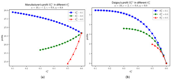
Figure 3. In Model D, manufacturer’s profit ${\mathsf{\Pi }}_m^{D\ast }$ and daigou’s profit ${\mathsf{\Pi }}_d^{D\ast }$ in different values of ${\theta }_m^D$, given that $a=10$, $b=2$, $\gamma =0.8$, and $\eta =0.8$. (a) ${\mathsf{\Pi }}_m^{D\ast }$. (b) ${\mathsf{\Pi }}_d^{D\ast }$.

In the following Figure 4, we have Model C manufacturer’s profit and daigou’s profit in different values of ${\theta }_m^C$.

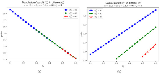
Figure 4. In Model C, manufacturer’s profit ${\mathsf{\Pi }}_m^{C\ast }$ and daigou’s profit ${\mathsf{\Pi }}_d^{C\ast }$ in different values of ${\theta }_m^C$, given that $a=10$, $b=2$, $\gamma =0.8$, $\eta =0.8$ and $Q=3$. (a) ${\mathsf{\Pi }}_m^{C\ast }$. (b) ${\mathsf{\Pi }}_d^{C\ast }$.

We see that Figure 3 and Figure 4 align with the monotonicity in Proposition 9. In each figure, we vary ${\theta }_m$ across $0.1$, $0.3$, and $0.5$ for comparison, selected with respect to the model’s asymmetric assumption that ${\theta }_m<{\theta }_d$. So, ${\theta }_d$ is plotted starting from values slightly above each corresponding ${\theta }_m$. Also, as the chosen effort parameters $\gamma =0.8$ and $\eta =0.8$, from Models D and C, we have ${\theta }_d<1-{\displaystyle \frac{{\gamma }^2}{2\eta }}=0.6$ in this case. Therefore, the upper limit of ${\theta }_d$ in the figures is ${\theta }_d=0.6$.

The following Figure 5 shows the daigou’s profit ${\mathsf{\Pi }}_d^{C\ast }$ against the quantity restriction $Q^C$, with different values ${\theta }_m^C$ for $a=10$, $c=2$, $\gamma =0.8$, and $\eta =0.8$. The figure aligns with the monotonicity of ${\mathsf{\Pi }}_d^{C\ast }$ in $Q^C$ as shown in Proposition 10.

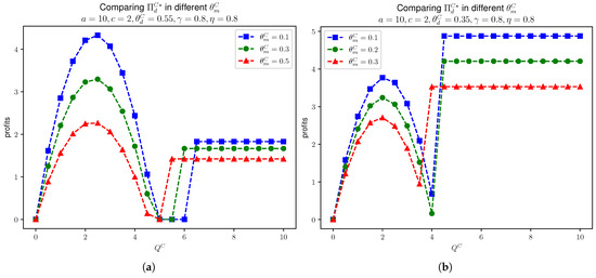
Figure 5. In Model C, manufacturer’s profit ${\mathsf{\Pi }}_m^{C\ast }$ and daigou’s profit ${\mathsf{\Pi }}_d^{C\ast }$ in different values of ${\theta }_m^C$, given that $a=10$, $b=2$, $\gamma =0.8$, $\eta =0.8$. (a) ${\theta }_d^C=0.55$. (b) ${\theta }_d^C=0.35$.

In Figure 6, we compare the manufacturer’s profit in Models D and C, given that $a=10$, $c=2$, ${\theta }_m=0.1$, $\gamma =0.8$ and $\eta =0.8$. We see that the manufacturer’s profit in Model C increases below the threshold for $Q^C$. For some loose $Q^C$, the manufacturer’s profit in Model C outperforms Model D. This illustration also confirms Proposition 7. A similar case is seen for daigou’s profit in Models D and C as shown in Figure 7. For Model C, when $Q^C$ is below the threshold, the daigou’s profit is quadratic with respect to $Q^C$. When the substitution rate ${\theta }_d=0.55$, we see that for tight values of $Q^C$, the daigou’s profit is larger than in Model D. This is because for the high substitution, consumers tend to purchase through daigou. Therefore, due to the tight value of $Q^C$, it creates the scarcity and, therefore, the price at daigou is higher. Hence, daigou’s profit in Model C outperforms that in Model D.

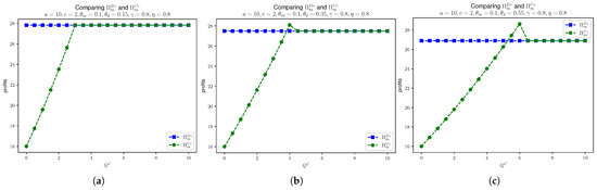
Figure 6. Comparing ${\mathsf{\Pi }}_m^{D\ast }$ and ${\mathsf{\Pi }}_m^{C\ast }$, given that $a=10$, $c=2$, ${\theta }_m=0.1$, $\gamma =0.8$ and $\eta =0.8$. (a) ${\theta }_d=0.15$. (b) ${\theta }_d=0.35$. (c) ${\theta }_d=0.55$.

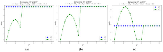
Figure 7. Comparing ${\mathsf{\Pi }}_d^{D\ast }$ and ${\mathsf{\Pi }}_d^{C\ast }$, given that $a=10$, $c=2$, ${\theta }_m=0.1$, $\gamma =0.8$ and $\eta =0.8$. (a) ${\theta }_d=0.15$. (b) ${\theta }_d=0.35$. (c) ${\theta }_d=0.55$.

7. Conclusions and Future Research

7.1. Conclusions

The daigou activities at Pang Donglai illustrate how daigou agents can increase sales for Pang Donglai. It also disrupts the traditional supply chain and reduces local customers from the manufacturer’s direct sales. The long queues outside Pang Donglai stores have made daigou one of the most effective and convenient channels for completing purchases. Such domestic daigou activities can generate additional sales opportunities for Pang Donglai, but at the same time, reduce local customers from the manufacturer’s direct sales. Also, it could flood the manufacturer’s direct sales capacity and therefore reduce its excellent customer service standards.

In conclusion, our study shows that daigou actually reduces channel conflicts. When comparing Model B and Model D, the manufacturer’s profit is higher in Model D. This outcome arises because daigou informally integrates into the supply chain, expanding market reach and generating additional revenue. Therefore, it enhances overall profitability for the manufacturer as daigou sources products directly from the manufacturer without discounts.

Constraints like purchase limits impact daigou and retailer strategies by balancing profitability with resilience. Compared to Model D, these limits in Model C reduce the manufacturer’s profit by reducing daigou’s purchase volumes and market expansion. However, for daigou, carefully chosen limits under specific conditions can increase their profits through supply scarcity and higher resale prices. More importantly, such constraints restrict daigou’s purchase quantity from the manufacturer. This ensures better service quality for regular consumers, improved inventory management, and stronger resilience against informal competition.

We also show that when daigou substitution dominates, ${\theta }_d>{\theta }_m$, it increases channel rivalry. It also disrupt the manufacturer profits in both unconstrained Model D and constrained Model C by shifting demand to informal channels. However, for daigou, higher ${\theta }_d$ initially enhances profits in Model D up to a threshold via better market segmentation. On the other hand, in Model C, it supports resilience through scarcity.

7.2. Limitations and Future Research

This study provides insights into strategic interactions in daigou activities; the findings are constrained by several simplifying assumptions. These include the following:

• In the models, this work considers only a single daigou in Models D and C; the current analysis does not consider multiple-daigou competition as multiple-daigou competition could cause price wars and reduce individual daigou profits.
• The models treat substitution effects as constant and asymmetric. It reduces the generalizability to scenarios where consumer preferences evolve dynamically, such as due to marketing or economic shifts. This may bias profit comparisons in the Propositions herein as it may downplay the impact of substitutions on channel conflicts and overall supply chain efficiency.
• The models are static and do not consider dynamic interactions over time. This may result bias toward short-term equilibria and constrain the applicability to long-term scenarios where daigou adaptation or manufacturer responses could alter profit thresholds.

The assumptions in the analysis were to ensure analytical tractability and focus on the core mechanisms of manufacturer–daigou strategies. There are also several areas that could be improved to better align the model with practical business scenarios. Therefore, future research could address these gaps by conducting the following:

• Exploring multi-agent dynamics and competition by incorporating multiple daigou agents to analyze intra-daigou rivalry, cooperation thresholds, and network effects on market equilibrium.
• Incorporate discrete choice models to segment consumers into local versus remote groups, analyzing preference heterogeneity, loyalty dynamics, and the efficacy of manufacturer counter-strategies such as targeted loyalty programs or personalized pricing to mitigate daigou.
• Develop time-dependent models that consider for inventory, seasonal demand variations, or supply chain uncertainties. It enables the optimization of adaptive purchase limits and resilience strategies in volatile global markets.
• Investigate how digital platforms can implement governance policies, such as algorithmic monitoring or incentive structures. So, it could regulate daigou activities, balance informal innovation with formal channel protection and exploring impacts on transaction efficiency and trust.
• Examine the role of government regulations, including tariffs and anti-gray market laws in shaping daigou ecosystems. Then, build the models where interventions could alter profit distributions and assess unintended consequences like supply chain disruptions.

7.3. Managerial Implications

7.3.1. Manufacturer

In the case when informal resale presents, manufacturers need to regard daigou not just as adversaries, it could also be potential business partners. The Daigou Entry Model illustrates how these agents can increase market access. We see that domestic daigou expands the market to remote or convenience-oriented consumers, which increases profit. Yet, this comes at a cost. Daigou activity risks the manufacturer’s direct sales profit, which is shown in Proposition 7. Therefore, good purchase limits in the Constrained Daigou Model can outperform Model D’s daigou profits when $Q^C$ is chosen within a certain range. Such limits can also bring the demand back to the direct channels. In practice, these constraints can be implemented through mechanisms like membership cards. The membership card record system can be used to restrict purchase quantities within a specified period because typical consumers do not repurchase identical items multiple times in short periods. This method can target daigou without unnecessarily harming regular consumers. Also, managers must constantly track substitution parameters and adjust constraints dynamically. This can reduce the influence from the daigou. Proposition 9 shows the urgency of stricter controls at high daigou substitution ${\theta }_d$. Early action can help preserve the consumer from direct channels. Managers learn to formalize daigou with partnership, therefore enhancing supply chain robustness.

7.3.2. Daigou

Daigou grows in the unrestricted Model D, whereby utilizing its effort and networks can increase the demand. In Proposition 7, a counterintuitive advantage is observed as a certain range of constraints in Model C yields higher profits via scarcity. Daigou should emphasize operational efficiency over raw volume, perhaps via niche customer ecosystems, to sustain earnings. Proposition 9 demonstrates that robust ${\theta }_d$ increases profits in Model C and even earlier in Model D. Furthermore, to enhance sustainability, daigou could explore formalization as authorized resellers. It could negotiate product discounts from manufacturers to legitimize arbitrage opportunities. Therefore, it can reduce risks associated with informal channels.

References

- Zhang, X.; Tham, A.; Liu, Y.; Spinks, W.; Wang, L. ‘To market, to market’: Uncovering Daigou touristscapes within Chinese outbound tourism. J. China Tour. Res. 2021, 17, 549–569. [Google Scholar] [CrossRef]
- Park, H.; Kim, S.; Jeong, Y.; Minshall, T. Customer entrepreneurship on digital platforms: Challenges and solutions for platform business models. Creat. Innov. Manag. 2021, 30, 96–115. [Google Scholar] [CrossRef]
- Zhuoxiao, X. Im/materializing cross-border mobility: A study of mainland China–Hong Kong Daigou (Cross-border shopping services on global consumer goods). Int. J. Commun. 2018, 12, 4052–4065. [Google Scholar]
- Zhu, Z.; Tang, X. Effect of integration capabilities with channel distributors on supply chain agility in emerging markets: An institution-based view perspective. J. Enterp. Inf. Manag. 2023, 36, 381–408. [Google Scholar] [CrossRef]
- Glavas, C.; Mortimer, G.; Ding, H.; Grimmer, L.; Vorobjovas-Pinta, O.; Grimmer, M. How entrepreneurial behaviors manifest in non-traditional, heterodox contexts: Exploration of the Daigou phenomenon. J. Bus. Ventur. Insights 2023, 19, e00385. [Google Scholar] [CrossRef]
- Kohn, M. Competitive speculation. Econom. J. Econom. Soc. 1978, 46, 1061–1076. [Google Scholar] [CrossRef]
- Tirole, J. On the possibility of speculation under rational expectations. Econom. J. Econom. Soc. 1982, 50, 1163–1181. [Google Scholar] [CrossRef]
- Courty, P. Some economics of ticket resale. J. Econ. Perspect. 2003, 17, 85–97. [Google Scholar] [CrossRef]
- Courty, P. Ticket pricing under demand uncertainty. J. Law Econ. 2003, 46, 627–652. [Google Scholar] [CrossRef]
- Geng, X.; Wu, R.; Whinston, A.B. Profiting from partial allowance of ticket resale. J. Mark. 2007, 71, 184–195. [Google Scholar] [CrossRef]
- Su, X. Optimal pricing with speculators and strategic consumers. Manag. Sci. 2010, 56, 25–40. [Google Scholar] [CrossRef]
- Lim, W.S.; Tang, C.S. Advance selling in the presence of speculators and forward-looking consumers. Prod. Oper. Manag. 2013, 22, 571–587. [Google Scholar] [CrossRef]
- Feng, T.; Geunes, J. Speculation in a two-stage retail supply chain. IIE Trans. 2014, 46, 1315–1328. [Google Scholar] [CrossRef]
- Huang, Y.S.; Gu, Y.H.; Fang, C.C. Pricing of perishable products with a speculator and strategic customers. Int. J. Syst. Sci. Oper. Logist. 2019, 6, 301–319. [Google Scholar] [CrossRef]
- Kuksov, D.; Liao, C. Restricting Speculative Reselling: When “How Much” Is the Question. Mark. Sci. 2023, 42, 377–400. [Google Scholar] [CrossRef]
- Zhao, K.; Zhao, X.; Deng, J. Online price dispersion revisited: How do transaction prices differ from listing prices? J. Manag. Inf. Syst. 2015, 32, 261–290. [Google Scholar] [CrossRef]
- Zhao, K.; Zhao, X.; Deng, J. An empirical investigation of online gray markets. J. Retail. 2016, 92, 397–410. [Google Scholar] [CrossRef]
- Bai, H.; McColl, J.; Moore, C. Luxury retailers’ entry and expansion strategies in China. Int. J. Retail Distrib. Manag. 2017, 45, 1181–1199. [Google Scholar] [CrossRef]
- Huang, H.; He, Y.; Chen, J. Competitive strategies and quality to counter parallel importation in global market. Omega 2019, 86, 173–197. [Google Scholar] [CrossRef]
- Zhang, Z.; Feng, J. Price of identical product with gray market sales: An analytical model and empirical analysis. Inf. Syst. Res. 2017, 28, 397–412. [Google Scholar] [CrossRef]
- Prasetyo, E.H. Digital platforms’ strategies in Indonesia: Navigating between technology and informal economy. Technol. Soc. 2024, 76, 102414. [Google Scholar] [CrossRef]
- Belk, R. You are what you can access: Sharing and collaborative consumption online. J. Bus. Res. 2014, 67, 1595–1600. [Google Scholar] [CrossRef]
- Schlagwein, D.; Schoder, D.; Spindeldreher, K. Consolidated, systemic conceptualization, and definition of the “sharing economy”. J. Assoc. Inf. Sci. Technol. 2020, 71, 817–838. [Google Scholar] [CrossRef]
- Marth, S.; Hartl, B.; Penz, E. Sharing on platforms: Reducing perceived risk for peer-to-peer platform consumers through trust-building and regulation. J. Consum. Behav. 2022, 21, 1255–1267. [Google Scholar] [CrossRef] [PubMed]
- Tang, W.; Xie, N.; Mo, D.; Cai, Z.; Lee, D.H.; Chen, X.M. Optimizing subsidy strategies of the ride-sourcing platform under government regulation. Transp. Res. Part E Logist. Transp. Rev. 2023, 173, 103112. [Google Scholar] [CrossRef]
- Liu, Y.; Wang, X.; Gilbert, S.; Lai, G. On the participation, competition and welfare at customer-intensive discretionary service platforms. Manuf. Serv. Oper. Manag. 2023, 25, 218–234. [Google Scholar] [CrossRef]
- Bai, J.; So, K.C.; Tang, C.S.; Chen, X.; Wang, H. Coordinating supply and demand on an on-demand service platform with impatient customers. Manuf. Serv. Oper. Manag. 2019, 21, 556–570. [Google Scholar] [CrossRef]
- Chen, X.M.; Zheng, H.; Ke, J.; Yang, H. Dynamic optimization strategies for on-demand ride services platform: Surge pricing, commission rate, and incentives. Transp. Res. Part B Methodol. 2020, 138, 23–45. [Google Scholar] [CrossRef]
- Benjaafar, S.; Kong, G.; Li, X.; Courcoubetis, C. Peer-to-peer product sharing: Implications for ownership, usage, and social welfare in the sharing economy. Manag. Sci. 2019, 65, 477–493. [Google Scholar] [CrossRef]
- Belleflamme, P.; Peitz, M. Platform competition: Who benefits from multihoming? Int. J. Ind. Organ. 2019, 64, 1–26. [Google Scholar] [CrossRef]
- Taylor, T.A. On-demand service platforms. Manuf. Serv. Oper. Manag. 2018, 20, 704–720. [Google Scholar] [CrossRef]
- Dong, J.; Ibrahim, R. Managing supply in the on-demand economy: Flexible workers, full-time employees, or both? Oper. Res. 2020, 68, 1238–1264. [Google Scholar] [CrossRef]
- Ert, E.; Fleischer, A.; Magen, N. Trust and reputation in the sharing economy: The role of personal photos in Airbnb. Tour. Manag. 2016, 55, 62–73. [Google Scholar] [CrossRef]
- Raju, S.; Rofin, T.; Kumar, S.P. Pricing strategies for dual-channel supply chain members under pandemic demand disruptions. Oper. Res. 2025, 25, 58. [Google Scholar] [CrossRef]
- Thaichon, P.; Quach, S.; Barari, M.; Nguyen, M. Exploring the role of omnichannel retailing technologies: Future research directions. Australas. Mark. J. 2024, 32, 162–177. [Google Scholar] [CrossRef]
- Radomska, J.; Kawa, A.; Hajdas, M.; Klimas, P.; Silva, S.C. Unveiling retail omnichannel challenges: Developing an omnichannel obstacles scale. Int. J. Retail Distrib. Manag. 2024, 53, 1–20. [Google Scholar] [CrossRef]
- Cai, Y.J.; Lo, C.K. Omni-channel management in the new retailing era: A systematic review and future research agenda. Int. J. Prod. Econ. 2020, 229, 107729. [Google Scholar] [CrossRef]
- Tan, Y. The first-ever e-commerce law: How will the law impact individuals and businesses. Tsinghua China L. Rev. 2022, 11, 427. [Google Scholar]
- Cachon, G.P.; Lariviere, M.A. Supply chain coordination with revenue-sharing contracts: Strengths and limitations. Manag. Sci. 2005, 51, 30–44. [Google Scholar] [CrossRef]
- Yang, H.; Luo, J.; Zhang, Q. Supplier encroachment under nonlinear pricing with imperfect substitutes: Bargaining power versus revenue-sharing. Eur. J. Oper. Res. 2018, 267, 1089–1101. [Google Scholar] [CrossRef]
- Matsui, K. Asymmetric product distribution between symmetric manufacturers using dual-channel supply chains. Eur. J. Oper. Res. 2016, 248, 646–657. [Google Scholar] [CrossRef]
- Huang, S.; Guan, X.; Chen, Y.J. Retailer information sharing with supplier encroachment. Prod. Oper. Manag. 2018, 27, 1133–1147. [Google Scholar] [CrossRef]
- Shao, J.; Krishnan, H.; McCormick, S.T. Gray markets and supply chain incentives. Prod. Oper. Manag. 2016, 25, 1807–1819. [Google Scholar] [CrossRef]
- Ahmadi, R.; Iravani, F.; Mamani, H. Coping with gray markets: The impact of market conditions and product characteristics. Prod. Oper. Manag. 2015, 24, 762–777. [Google Scholar] [CrossRef]
- Hong, D.; Sheng, J.; Wu, Z.; Fan, J. Authorized retailer’s gray market activities and supply chain performance improvement. J. Ind. Manag. Optim. 2025, 21, 7161–7185. [Google Scholar] [CrossRef]
- Chiang, W.y.K.; Chhajed, D.; Hess, J.D. Direct marketing, indirect profits: A strategic analysis of dual-channel supply-chain design. Manag. Sci. 2003, 49, 1–20. [Google Scholar] [CrossRef]
- Tsay, A.A.; Agrawal, N. Channel conflict and coordination in the e-commerce age. Prod. Oper. Manag. 2004, 13, 93–110. [Google Scholar] [CrossRef]
- Taylor, T.A. Supply chain coordination under channel rebates with sales effort effects. Manag. Sci. 2002, 48, 992–1007. [Google Scholar] [CrossRef]
- Krishnan, H.; Kapuscinski, R.; Butz, D.A. Coordinating contracts for decentralized supply chains with retailer promotional effort. Manag. Sci. 2004, 50, 48–63. [Google Scholar] [CrossRef]
- Gurnani, H.; Erkoc, M. Supply contracts in manufacturer-retailer interactions with manufacturer-quality and retailer effort-induced demand. Nav. Res. Logist. (NRL) 2008, 55, 200–217. [Google Scholar] [CrossRef]
- Ma, P.; Wang, H.; Shang, J. Supply chain channel strategies with quality and marketing effort-dependent demand. Int. J. Prod. Econ. 2013, 144, 572–581. [Google Scholar] [CrossRef]
- Tsay, A.A.; Agrawal, N. Channel dynamics under price and service competition. Manuf. Serv. Oper. Manag. 2000, 2, 372–391. [Google Scholar] [CrossRef]
- Han, F.; Wang, M.; Wu, Z. Information sharing and channel structure in e-commerce supply chain considering data-driven marketing. PLoS ONE 2025, 20, e0328040. [Google Scholar] [CrossRef] [PubMed]
Disclaimer/Publisher’s Note: The statements, opinions and data contained in all publications are solely those of the individual author(s) and contributor(s) and not of MDPI and/or the editor(s). MDPI and/or the editor(s) disclaim responsibility for any injury to people or property resulting from any ideas, methods, instructions or products referred to in the content. |
© 2025 by the authors. Licensee MDPI, Basel, Switzerland. This article is an open access article distributed under the terms and conditions of the Creative Commons Attribution (CC BY) license (https://creativecommons.org/licenses/by/4.0/).