Article

Modified Heisenberg Commutations Relations and Its Standard Hamiltonian Interpretation

by
Mauricio Contreras González
1,
Roberto Ortiz Herrera
2,3,* and
José Mauricio González
1
1
Departamento de Física y Astronomía, Universidad Andres Bello, Sazié 2212, Chile
2
Facultad de Ingeniería y Ciencias, Universidad Diego Portales, Santiago 8370191, Chile
3
Facultad de Ciencias Económicas y Administrativas FACEA, Universidad Católica de la Santísima Concepción, Concepción 4070129, Chile
*
Author to whom correspondence should be addressed.
Mathematics 2025, 13(23), 3872; https://doi.org/10.3390/math13233872
Submission received: 7 October 2025 / Revised: 18 November 2025 / Accepted: 30 November 2025 / Published: 3 December 2025

Abstract

This paper analyzes the modified canonical Heisenberg commutation relations or GUP, from a standard Hamiltonian point of view. For a one-dimensional system, a such modified canonical Heisenberg commutation relation is defined by the commutator between a position x ^ and a momentum operator p ^ (called the deformed momentum), which becomes a function F of the same operators: x ^ , p ^ = F ( x ^ , p ^ ) , that is, the Heisenberg algebra closes itself in general in a nonlinear way. The function F also depends on a parameter that controls the deformation of the Heisenberg algebra in such a way that for a null parameter value, one recovers the usual Heisenberg algebra x ^ , p ^ 0 = i I . Thus, it naturally raises the following questions: What does a relation of this type mean in Hamiltonian theory from a standard point of view? Is the deformed momentum the canonical variable conjugate to the position in such a relation? Moreover, what are the canonical variables in this model? The answer to these questions comes from the existence of two different phase spaces: The first one, called the non-deformed phase (which is obtained for control parameter value equal to zero), is defined by the Cartesian x ^ coordinate and its non-deformed conjugate momentum p ^ 0 , which satisfies the standard quantum mechanical Heisenberg commutation relation. The second phase space, the deformed one, is given by the deformed momentum p ^ and a new position coordinate y ^ , which is its canonical conjugate variable, so y ^ and p ^ also satisfy standard commutation relations. We construct a classical canonical transformation that maps the non-deformed phase space into the deformed one for a specific class of deformation functions F. Additionally, a quantum mechanical operator transformation is found between the two non-commutative phase spaces, which allows the Schrödinger equation to be written in both spaces. Thus, there are two equivalent quantum mechanical descriptions of the same physical process associated with a deformed commutation relation.

1. Introduction

In recent years, there has been growing interest in studying possible modifications to the usual canonical commutation relations
x ^ , p ^ = x ^ p ^ p ^ x ^ = i I .
in various contexts. For example, it is well known that quantum gravity effects, modeled by string theory, loop quantum gravity, or black hole physics, predict the existence of a generalized uncertainty principle (GUP), which can change the usual canonical commutation relations [1,2,3,4,5,6,7,8,9,10,11,12,13] and its possible implications for entanglement [14,15,16,17,18,19].
In this case, the canonical commutation relations (1) are replaced by a more general one, of the type
[ x ^ , p ^ ] = i F ( x ^ , p ^ )
for some function F ( x , p ) depending on the position and momentum. The form of the quantum algebra (2) guarantees that the system has a classical limit when goes to zero. Usually in quantum mechanics, it is assumed that the momentum p ^ and the position x ^ operators are Hermitian ( p ^ = p ^ , x ^ = x ^ ) in order for its eigenvalues to be real. Additionally, they are well defined over an open set of the real axis, which could be the entire real axis. By expanding the function F to first order, we obtain the following expression:
[ x ^ , p ^ ] = i F ( 0 , 0 ) I + α x ^ + β p ^ +
In this context, the parameters α and β can be considered as control parameters that quantify the degree of deformation of the Heisenberg algebra (2) in relation to the standard case (1). To recover the usual Heisenberg commutation relation (1) in the limit α 0 and β 0 , the function F must satisfy the condition F ( 0 , 0 ) = 1 .
To study the effects of an algebra of the form (2), one can consider some particular forms of the F function. For simplicity, in this paper we consider the cases F ( x , p ) = f ( x ) and F ( x , p ) = g ( p ) , so the modified Heisenberg commutation relation reads
x ^ , p ^ = i f ( x ^ )
or
x ^ , p ^ = i g ( p ^ )
where we assume that f ( x ) and g ( p ) are analytical functions defined over the entire real axis or a subset of real numbers, with f ( 0 ) = 1 and g ( 0 ) = 1 . An interesting example is the case of a linear function f ( x ) = 1 + α x , as well as g ( p ) = 1 + β p , which can be analyzed further. In general, the functions f and g would depend also on a control variable (such as the α or β parameter) in such a way that when α , β goes to zero, then f , g also goes to zero, and one recovers the standard commutation relation (1) in this limit. Thus, the control variable essentially measures the degree of deformation of the GUP relation in a continuous way.
The implications of these modified Heisenberg commutation relations over another simple one-dimensional system, specifically on the infinite square-well potential, can be found in [20,21,22,23,24,25,26,27,28]. In [29], an analysis of the impact of the deformation of the Heisenberg algebra on the properties of free waves and the tunneling effect was carried out. It was also demonstrated that a special type of deformed algebra is related to the Black–Scholes equation in finance theory.
In all these studies, no further mention is made of the interpretation, from a strictly Hamiltonian point of view, of these deformed commutation relations. Thus, the following questions naturally arise: What does a relation of type (2), (4) or (5) mean in Hamiltonian theory? Is the momentum p the canonical variable conjugate to the position x? What are the canonical variables in this model in a standard sense?
This paper aims to answer these questions and understand what deformed commutation relations mean from a standard Hamiltonian perspective at both classical and quantum levels. The main finding is the existence of two distinct phase spaces associated with a deformed commutation relation of the type (4) and (5).
The first is called the non-deformed phase space, where the deformation parameters α , β are set to zero, or where f = 1 or g = 1 in Equations (4) and (5). The second phase space, the deformed one, is characterized by non-zero values of α , β , or where f 1 or g 1 .
Of course, both phase spaces coincide when the Heisenberg algebra is non-deformed; however, as the deformation parameters gradually increase from zero, these phase spaces begin to diverge.
We prove here that both phase spaces are equivalent from a physical point of view, which means that they are (i) classically equivalent and (ii) they are equivalent at the quantum level.
To prove (i), we construct a canonical transformation that connects deformed and non-deformed classical phase spaces.
To prove (ii), we use the same classical transformation to induce a quantum transformation that maps the momentum and position operators of the non-deformed quantum phase space to the deformed ones. In this way, one can build two quantum equivalent theories (both characterized by standard commutation relations) that describe the same system.
The above results, from a mathematical point of view, are equivalent to stating that the deformed Heisenberg algebras (4) and (5) are hybrid objects, which combine operators from two distinct sets. For example, consider two different set of operators A = { x ^ 1 , p ^ 1 } and B = { x ^ 2 , p ^ 2 } that satisfy standard Heisenberg algebras
[ x ^ 1 , p ^ 1 ] = i I , [ x ^ 2 , p ^ 2 ] = i I
If these operator sets are not independent, then the commutators between them cannot be trivial. For example, one could write
[ x ^ 1 , p ^ 2 ] = i F ( x ^ 1 , p ^ 1 , x ^ 2 , p ^ 2 )
which is a hybrid object, because it contains operators from both sets. However, Equation (7) is just a type of GUP relation. In this paper, we reverse the process, constructing the operator sets A and B that satisfy relations (6) from a GUP of the form (7).
Thus, one can write a Schrödinger equation in both spaces. As we see later, for the case of the GUP algebra (5), for a non-relativistic Hamiltonian operator, the Schrödinger equation in one phase space becomes an infinite-order PDE. In contrast, in the other phase space, it becomes a finite-order PDE. Then, the quantum transformation can be of interest to mathematicians who are interested in such infinite-order PDEs.
This paper is organized as follows: Section 2 analyzes the case of nonlinear deformation in position, for F ( x , p ) = f ( x ) . It presents the classical canonical transformation between the non-deformed and deformed phase spaces, which will be used in the same section to construct a quantum mechanical operator transformation between the quantum phase spaces. A discussion on the hermiticity of the deformed momentum is carried out. Also, this section presents, as a specific example, the case of a linear deformation in position. Following this, the corresponding Schrödinger equation is derived in both spaces.
Section 3 address similar issues for both nonlinear and linear momentum deformation cases F ( x , p ) = g ( p ) . In Section 4, the implications of the deformed Heisenberg commutation relation at the classical level are examined for a well-known system: the harmonic oscillator. Finally, Section 5 provides a conclusion for this work.

2. The Nonlinear f ( x ^ ) Deformation Case

Consider now the nonlinear deformed Heisenberg algebra (4) for a one-variable function f ( x ) . This algebra has a non-Hermitian representation
x ^ = x
p ^ = f ( x ^ ) p ^ 0 = i f ( x ) x
where p ^ 0 = i x is the standard non-deformed momentum operator, which satisfies the commutation relations
x ^ , p ^ 0 = i I
The eigenfunctions Φ p of the deformed momentum p ^ are the solutions of the equation
p ^ Φ p = i f ( x ) Φ p x = p Φ p
that is
Φ p = A e i p Θ ( x )
with Θ ( x ) = d x f ( x ) . From the momentum eigenstate (12), one would identify the classical variable y = Θ ( x ) as the canonical conjugate coordinate to the classical deformed momentum p. In a physical sense, the y coordinate is the spatial coordinate, for which the deformed eigenstate Φ p = A e i p y appears as a free quantum wave.

2.1. Classical Aspects

Thus, the variables ( x , p 0 ) define the non-deformed phase space, whereas ( y , p ) would define the deformed one, classically. Now, by taking the classical limit 0 , one hopes that the quantum operators go to their classical counterparts, that is, x ^ x , p ^ p and p ^ 0 p 0 , so (9) implies that p ^ p = f ( x ) p 0 .
Theorem 1. 
The following transformation, between the non-deformed ( x , p 0 ) phase space to the deformed ( y , p ) phase space, given by
p = p ( x , p 0 ) = f ( x ) p 0
y = y ( x , p 0 ) = Θ ( x ) ,
is a canonical transformation.
Proof. 
Let { A , B } 0 be the Poisson bracket defined on the non-deformed space ( x , p 0 ) , that is
{ A , B } 0 = A x B p 0 B p 0 A x
Then one has, according to (13) and (14),
{ y , p } 0 = y x p p 0 y p 0 p x = x ( Θ ( x ) ) p 0 ( f ( x ) p 0 ) = 1 f ( x ) f ( x ) = 1
That is, y and p are classical canonical variables. The other Poisson brackets between the canonical variables are
{ x , p 0 } 0 = 1
{ x , p } 0 = f ( x )
{ p , p 0 } 0 = f ( x ) p 0
{ y , p 0 } 0 = 1 f ( x )

2.2. Quantum Aspects

We consider here the quantum version of the classical transformation constructed in the previous subsection. Thus, we can state the following theorem:
Theorem 2. 
There exist two quantum operator sets A = { x ^ , p ^ 0 } and B = { y ^ , p ^ } , that satisfy standard Heisenberg algebras
[ x ^ , p ^ 0 ] = i I , [ y ^ , p ^ ] = i I
and also satisfy the GUP relation
x ^ , p ^ = i f ( x ^ )
Proof. 
For the operators in the set A = { x ^ , p ^ 0 } , consider the representation
x ^ = x , p ^ 0 = i x
which, of course, satisfies [ x ^ , p ^ 0 ] = i I . Consider now the following deformed quantum operators y ^ and p ^ in the B set, defined according to
p ^ = f ( x ^ ) p ^ 0
y ^ = Θ ( x ^ )
then
y ^ , p ^ = Θ ( x ^ ) , f ( x ^ ) p ^ 0 = Θ ( x ^ ) f ( x ^ ) p ^ 0 f ( x ^ ) p ^ 0 Θ ( x ^ ) = f ( x ^ ) Θ ( x ^ ) , p ^ 0
but
Θ ( x ^ ) , p ^ 0 = i d Θ ( x ^ ) d x = i f ( x ^ )
so
y ^ , p ^ = f ( x ^ ) i f ( x ^ ) = i I
Also,
x ^ , p ^ = x ^ , f ( x ^ ) p ^ 0 = f ( x ^ ) x ^ , p ^ 0 = i f ( x ^ )
The other commutators are
p ^ , p ^ 0 = f ( x ^ ) p ^ 0 , p ^ 0 = f ( x ^ ) p ^ 0 p ^ 0 p ^ 0 f ( x ^ ) p ^ 0 = f ( x ^ ) , p ^ 0 p ^ 0 = i f ( x ^ ) p ^ 0
and
y ^ , p ^ 0 = Θ ( x ^ ) , p ^ 0 = i f ( x ^ )
Thus, the full quantum algebra is given by
x ^ , p ^ 0 = i I y ^ , p ^ = i I x ^ , p ^ = i f ( x ^ ) p ^ , p ^ 0 = i f ( x ^ ) p ^ 0 y ^ , p ^ 0 = i f ( x ^ )
Note that, in terms of the non-deformed and deformed quantum phase spaces, the GUP relation (4) becomes a hybrid object, because it contains variables from different quantum phase spaces.

2.3. Dynamical Aspects and Schrödinger’s Equation

To study the system’s dynamical behavior associated with the quantum mechanical relation (4), one needs the classical Hamiltonian H ( x , p ) , which for a non-relativistic classical particle would be
H x , p = p 2 2 m + U ( x )
Note that the above Hamiltonian is a hybrid object because it contains variables from different classical phase spaces. If one considers the deformed ( y , p ) classical phase space, the Hamiltonian function is
H y , p = p 2 2 m + U ( Θ 1 ( y ) )
where Θ 1 is the inverse function of Θ . The quantization of this classical Hamiltonian by the standard commutation relation rule
y ^ , p ^ = i I
gives the following time-independent Schrödinger equation
2 2 m 2 Ψ ( y ) y 2 + U ( Θ n 1 ( y ) ) Ψ ( y ) = E Ψ ( y )
Instead, in the ( x , p 0 ) phase space, the Hamiltonian is just (23) with p = f ( x ) p 0 . The quantization in this space can be carried out by using the GUP relation (4) for x ^ and p ^ , by means of the representation (8) and (9), which implies the following Schrödinger equation:
2 2 m f ( x ) x f ( x ) Ψ ( x ) x + U ( x ) Ψ ( x ) = E Ψ ( x )
or
2 2 m f ( x ) 2 2 Ψ ( x ) x 2 + f ( x ) f ( x ) Ψ ( x ) x + U ( x ) Ψ ( x ) = E Ψ ( x )
Through this paper we use a right-quantization operator ordering, that is, for a classical product of the form p = f ( x ) p 0 = p 0 f ( x ) , the quantization procedure places the derivative operator to the right-side: p ^ = i f ( x ) x . Of course, one can take other operator orderings, which will give different Schrödinger equations. With the right-side operator ordering, we can state the following theorem:
Theorem 3. 
The Schrödinger’s Equations (26) and (27) associated with the deformed and non-deformed phase spaces are equivalent.
Proof. 
To map Equation (26) to the ( x , p 0 ) phase space, one uses the transformation (14) so
y = Θ ( x ) x x = f ( x ) x
and
2 y 2 = f ( x ) x f ( x ) x ,
and by replacing the second derivatives and using (14) in Equation (26), one obtains (27). □

2.4. Some Probabilistic Aspects

Now, we consider the probabilistic interpretation of the wave function in both phase spaces. Let Ψ ( y ) be a solution of the time-independent Schrödinger equation for some fixed energy E, and the probability density is, then,
ρ ( y ) = Ψ * ( y ) Ψ ( y ) = | Ψ ( y ) | 2
and the probability of finding the particle between y = a and y = b is
P ( a < y < b ) = a b Ψ * ( y ) Ψ ( y ) d y
To obtain the corresponding probability in terms of the x variable, one can use the transformation (13), so d y = d Θ ( x ) d x d x = d x f ( x ) and
P ( a < y < b ) = a b Ψ * ( y ) Ψ ( y ) d y = c d Ψ * Θ ( x ) Ψ Θ ( x ) d x f ( x )
with c = Θ 1 ( a ) and d = Θ 1 ( b ) .
One sees then, that in ( x , p 0 ) phase space, there exists an effective wave function Ψ ˜ defined by
Ψ ˜ ( x ) = Ψ Θ ( x ) f ( x )
so the probability density in terms of x is
ρ ( x ) = Ψ ˜ * ( x ) Ψ ˜ ( x ) = | Ψ ˜ ( x ) | 2 = Ψ * Θ ( x ) Ψ Θ ( x ) f ( x )
where Ψ Θ ( x ) denotes the solution Ψ ( y ) obtained in ( y , p ) phase space evaluated at y = Θ ( x ) . Also, the standard internal product in the ( y , p ) phase space
< Ψ 1 ( y ) , Ψ 2 ( y ) > = + Ψ 1 * ( y ) Ψ 2 ( y ) d y
will be mapped to the ( x , p 0 ) phase space according to
< Ψ ˜ 1 ( x ) , Ψ ˜ 2 ( x ) > = + Ψ ˜ 1 * ( x ) Ψ ˜ 2 ( x ) d x
with Ψ ˜ ( x ) = Ψ ( x ) f ( x ) , and where Ψ ( x ) is a solution of the the time-independent Schrödinger Equation (27).
One can ask the following question: Why is the probability density not directly the square modulus of the solutions Ψ ( x ) of the Schrödinger Equation (27)? Why is the re-normalization factor 1 f ( x ) necessary? This problem is related to the fact that the representation for our deformed momentum p ^ in (9) is not Hermitian.

2.5. The Hermitian Momentum Operator

Consider the Heisenberg commutation relation (10). Let p ^ 0 be the operator defined by
p ^ 0 = p ^ 0 + K I
where K is a complex constant and where p ^ 0 = p ^ 0 . Then,
x ^ , p ^ 0 = x ^ , p ^ 0 + K I = x ^ , p ^ 0 = i I
Thus, p ^ 0 and p ^ 0 satisfy the same commutation relations (10), that is, the momentum operator is not determined in a unique way from (10). Note that
p ^ 0 = p ^ 0 + K * I = p ^ 0 + K * I p ^ 0 ,
so p ^ 0 is not an Hermitian operator if K is a complex number. But the operator
p ^ 0 = p ^ 0 + p ^ 0 2 = p ^ 0 + ( K + K * ) 2 I
is Hermitian and also satisfies (10). Thus, one can always find a whole family of Hermitian operators that satisfy the Heisenberg commutation relations (10). The same can be said for the commutation relation (4). In this case, the momentum operator defined in (18) is not a Hermitian operator; in fact,
p ^ = f ( x ^ ) p ^ 0 = p ^ 0 f ( x ^ ) = p ^ 0 f ( x ^ ) = p ^ 0 f ( x ^ )
Now,
p ^ ψ ( x ) = p ^ 0 f ( x ^ ) ψ ( x ) = i x f ( x ) ψ ( x ) = i f ( x ) ψ ( x ) i f ( x ) ψ ( x ) x = i f ( x ) ψ ( x ) + f ( x ) p ^ 0 ψ ( x ) = i f ( x ) ψ ( x ) + p ^ ψ ( x )
Thus,
p ^ = p ^ i f ( x ^ )
A Hermitian representation for the momentum operator is, then,
p ^ H = p ^ + p ^ 2 = p ^ i f ( x ^ ) 2 = i f ( x ) x i 2 f ( x ) = i f ( x ) x + 1 2 f ( x )
Theorem 4. 
The eigenstates Φ ˜ p and Φ p of the Hermitian p ^ H and non-hermitian p ^ momentum operators, respectively, are related by
Φ ˜ p ( x ) = Φ p ( x ) f ( x )
Proof. 
The eigenstates of the non-Hermitian deformed momentum operator p ^ are defined by (11) and given by (12) as
Φ p ( x ) = A e i p Θ ( x )
The eigenstates of the Hermitian deformed momentum operator p ^ H are defined by
p ^ H Φ ˜ p = p Φ ˜ p
that is
i f ( x ) Φ ˜ p x i 2 f ( x ) Φ ˜ p = p Φ ˜ p
1 Φ ˜ p Φ ˜ p x = f ( x ) 2 f ( x ) + p i f ( x )
ln Φ ˜ p x = 1 2 ln f ( x ) x + i p Θ ( x ) x
thus
ln Φ ˜ p = 1 2 ln f ( x ) + i p Θ ( x ) + ln ( A )
or
Φ ˜ p ( x ) = A e i p Θ ( x ) f ( x ) = Φ p ( x ) f ( x )
Thus, the eigenstates of the Hermitian momentum are automatically normalized in the standard inner product (29).
Theorem 5. 
Let Ψ be the wave function associated with the non-Hermitian Schrödinger Equation (27)
1 2 m p ^ 2 Ψ + U ( x ) Ψ = E Ψ
Then, the normalized wave function, Ψ ˜ = Ψ f ( x ) , satisfies the Hermitian Schrödinger equation:
1 2 m p ^ H 2 Ψ ˜ + U ( x ) Ψ ˜ = E Ψ ˜
Proof. 
The action of the non-Hermitian deformed momentum operator over any state Ψ is
p ^ Ψ ( x ) = i f ( x ) Ψ ( x ) x
Thus, in terms of Ψ ˜ = Ψ f ( x ) , one has
p ^ Ψ ( x ) = i f ( x ) x ( f ( x ) Ψ ˜ ) = i f ( x ) f ( x ) 2 f ( x ) Ψ ˜ + f ( x ) Ψ ˜ x = i f ( x ) f ( x ) x + 1 2 f ( x ) Ψ ˜ = f ( x ) p ^ H Ψ ˜
Then,
p ^ 2 Ψ ( x ) = p ^ ( p ^ Ψ ) = p ^ ( f ( x ) p ^ H Ψ ˜ ) = f ( x ) p ^ H f ( x ) ( p ^ H Ψ ˜ ) f ( x ) = f ( x ) p ^ H ( p ^ H Ψ ˜ ) = f ( x ) p ^ H 2 Ψ ˜
Thus, the time-independent Schrödinger equation associated with the non-Hermitian momentum operator
1 2 m p ^ 2 Ψ + U ( x ) Ψ = E Ψ
can be written in terms of Ψ ˜ by using (31), as follows:
1 2 m f ( x ) p ^ H 2 Ψ ˜ + U ( x ) f ( x ) Ψ ˜ = E f ( x ) Ψ ˜
or
1 2 m p ^ H 2 Ψ ˜ + U ( x ) Ψ ˜ = E Ψ ˜
Note that in an explicit way, Equation (30) reads
2 2 m f ( x ) 2 2 x 2 + 2 f ( x ) f ( x ) x + ( 1 4 f ( x ) 2 + 1 2 f ( x ) f ( x ) ) Ψ ˜ + U ( x ) Ψ ˜ = E Ψ ˜

2.6. Physical Equivalence of Spectra in Both Representations

Consider the expectation value (at some state Ψ ) of the Hamiltonian operator associated with the classical Hamiltonian function (24) in the ( y , p ) phase space, that is
E = Ψ | H ^ | Ψ = a b Ψ * ( y ) 2 2 m 2 y 2 + U ( Θ n 1 ( y ) ) Ψ ( y ) d y
By using transformation (14), this quantity moves to the ( x , p 0 ) space
E = Ψ | H ^ | Ψ = c d Ψ * ( x ) 2 2 m f ( x ) 2 2 x 2 + f ( x ) f ( x ) x + U ( x ) Ψ ( x ) 1 f ( x ) d x
or
E = c d Ψ * ( x ) 1 2 m p ^ 2 Ψ ( x ) 1 f ( x ) d x + c d Ψ * ( x ) U ( x ) Ψ ( x ) 1 f ( x ) d x
Note that in the above equation we use the non-Hermitian deformed momentum p ^ , but a scalar product with weight factor w ( x ) = 1 f ( x ) . If, instead, one uses the wave function Ψ ˜ = Ψ f ( x ) , one obtains
E = c d Ψ ˜ * ( x ) 1 2 m p ^ 2 Ψ 1 f ( x ) d x + c d Ψ ˜ * ( x ) U ( x ) Ψ ˜ d x
but, due to Equation (31), one obtains
E = c d Ψ ˜ * ( x ) f ( x ) 1 2 m p ^ H 2 Ψ ˜ 1 f ( x ) d x + c d Ψ ˜ * ( x ) U ( x ) Ψ ˜ d x
that is
E = c d Ψ ˜ * ( x ) 1 2 m p ^ H 2 + U ( x ) Ψ ˜ d x
Thus, the eigenvalue E associated with an eigenstate of the Hamiltonian in the ( y , p ) phase space and the eigenvalue E associated with an eigenstate of the Hamiltonian in the ( x , p 0 ) phase space are identical. In the last case, the energy eigenvalue can be written in terms of a non-Hermitian deformed momentum operator p ^ ; however, the inner product needs to be renormalized by a weight factor of 1 f ( x ) . Alternatively, one can utilize a Hermitian momentum representation p ^ H and a tilde wave function in the standard inner product.
Also, one can analyze this problem from the point of view of the of the Sturm–Liouville theory. Note that the operator
o ^ = f ( x ) 2 2 x 2 + f ( x ) f ( x ) x
that appears in Equation (33) is a second-order differential operator. Now, according to the Sturm–Liouville theory, any second-order differential operator O ^ of the form
O ^ = a ( x ) 2 x 2 + b ( x ) x + c ( x ) ,
which is not necessary self-adjoint, can be converted in a self-adjoint operator by means of the integrating factor
w ( x ) = 1 a ( x ) e b ( x ) a ( x ) d x
in such a way that the operator
O ^ H = w ( x ) O ^
becomes self-adjoint. For the case that O ^ = o ^ , one has that a ( x ) = f ( x ) 2 and b ( x ) = f ( x ) f ( x ) , so the integration factor is
w ( x ) = 1 f 2 ( x ) e f 2 ( x ) f ( x ) f ( x ) d x = 1 f 2 ( x ) e f ( x ) f ( x ) d x = 1 f 2 ( x ) e d ln ( f ( x ) ) d x d x = 1 f ( x )
Then, the operator
o ^ H = w ( x ) o ^ = 1 f ( x ) f ( x ) 2 2 x 2 + f ( x ) f ( x ) x = f ( x ) 2 x 2 + f ( x ) x
is self-adjoint. Thus, the weight factor w ( x ) = 1 f ( x ) present in Equation (33) means that the non-Hermitian o ^ operator becomes Hermitian. Note that in the context of the Sturm–Liouville, there is no information about the linear momentum operator p ^ , only p ^ 2 .
We want to recall here that in the deformed commutation relation (4), x ^ represents the position operator in a Cartesian coordinate system, and p ^ becomes a function of the non-deformed p ^ 0 operator. Thus, the phase space ( x , p 0 ) represents the correct system for physically measurable quantities. It is interesting to note that the energy spectrum in terms of deformed momentum is not symmetric, which has several consequences, as discussed in [28]. For the evaluation of eigenvalues or probability densities, the choice of phase space is just a matter of preference. In the cases studied in the paper below, the probability amplitude is mathematically simpler in terms of the ( y , p ) phase space.
In summary, a deformed commutation relation, such as those represented by (4), is equivalent to two pairs of canonically quantum operators: y ^ , p ^ and x ^ , p ^ 0 which satisfy standard non-deformed commutation relations. Each pair generates a phase space in which the system can be described at both classical and quantum levels. Notably, the transformations given by (18) and (19) demonstrate that these descriptions are completely equivalent for the F ( x , p ) = f ( x ) case.

2.7. Example: The Linear x ^ Deformation Case

As a specific example, consider the linear deformation case, for which f ( x ) = 1 + α x , so the commutation relations are
x ^ , p ^ = i ( I + α x ^ )
The real α parameter essentially measures the deformation of (34) from the standard Heisenberg commutation relation (1). To obtain the quantum mechanics associated with this deformed commutation relation, one must quantize the classical Hamiltonian (23) by using the representation
x ^ = x p ^ = ( 1 + α x ) p ^ 0 = i ( 1 + α x ) x
which satisfies (34). The corresponding time-independent Schrödinger equation is, then,
2 2 m α ( 1 + α x ) Ψ ( x ) x + ( 1 + α x ) 2 2 Ψ ( x ) x 2 + U ( x ) Ψ ( x ) = E Ψ ( x )
The deformed momentum eigenstates Φ p in this case are given by p ^ Φ p ( x ) = p Φ p ( x ) , that is
i ( 1 + α x ) Φ p ( x ) x = p Φ p ( x )
which can be determined by integrating the above equation, so
Φ p ( x ) = C ( 1 + α x ) i p α = C e i p α ln ( 1 + α x ) = C e i p 1 α ln ( 1 + α x )
with C being a normalization constant.

2.7.1. Induced Classical Mechanics

In classical terms, one can interpret the variable
y = 1 α ln ( 1 + α x )
in (37) as a canonical conjugate of the deformed momentum p, that is, the eigenstate Φ p ( y ) = C e i p y corresponds to a free wave function in a ( y , p ) phase space. Also, in the classical limit 0 , the quantum relation (35) for the momentum goes to the classical one
p = ( 1 + α x ) p 0
Relations (38) and (39) induce a phase space transformation ( x , p 0 ) ( y , p ) between the classical deformed and non-deformed phase spaces which is canonical, that is,
{ y , p } 0 = y x p p 0 y p 0 p x = x 1 α ln ( 1 + α x ) p 0 ( 1 + α x ) p 0 = 1
Thus, these deformed and non-deformed classical phase spaces are characterized by the set of Poisson brackets:
{ x , p 0 } 0 = 1
{ y , p } 0 = { y , p } = 1
{ x , p } 0 = 1 + α x
{ p , p 0 } 0 = α p 0
{ y , p 0 } 0 = 1 ( 1 + α x )

2.7.2. The Quantum Algebra

In quantum terms, these phase spaces can be characterized as follows: consider the non-deformed quantum space ( x ^ , p ^ 0 ) which satisfies the algebra (10). Now define the deformed quantum operators p ^ and y ^ according to (obviously induced by its classical counterparts)
p ^ = ( 1 + α x ^ ) p ^ 0
y ^ = 1 α ln ( 1 + α x ^ )
Now, given the operators defined in (40) and (41), the phase-space operators y ^ , p ^ , x ^ , and p ^ 0 satisfy the following quantum algebra:
x ^ , p ^ 0 = i I
x ^ , p ^ = i ( I + α x ^ )
y ^ , p ^ = i I
p ^ , p ^ 0 = i α p ^ 0
y ^ , p ^ 0 = i ( 1 + α x ^ ) = i ( 1 + α x ^ ) 1
Note that y ^ and p ^ satisfy standard non-deformed commutation relations.

2.7.3. The Phase Spaces and the Schrödinger Equation

Thus, the quantum mechanical problem induced by the deformed Heisenberg commutation relation (34) can be analyzed in two different quantum phase spaces:
(i) The non-deformed ( α = 0 ) quantum phase space ( x ^ , p ^ 0 ) , in which the Schrödinger equation is given by (36) and where the deformed momentum (40) must be interpreted as a function of the quantum phase space variables ( x ^ , p ^ 0 ) .
(ii) The deformed ( α 0 ) quantum space ( y ^ , p ^ ) , in which the deformed canonical variables satisfy the usual Heisenberg commutation relations.
The classical Hamiltonian in this last frame can be obtained from (23) by solving x in terms of y through of Equation (38), that is,
x = e α y 1 α
Thus, the classical Hamiltonian function in the modified phase space ( y , p ) is
H y , p = p 2 2 m + U ( e α y 1 α )
Quantum theory can be obtained by using the standard representation of the canonical Heisenberg commutation relation (25), that is,
y ^ = y p ^ = i y
Thus, one arrives in this case at the following time-independent Schrödinger equation:
2 2 m 2 Ψ ( y ) y 2 + U e α y 1 α Ψ ( y ) = E Ψ ( y )
The Schrödinger Equation (46) can be mapped to the ( x , p 0 ) phase space by means of transformation (38), which implies that
2 y 2 = ( 1 + α x ) x ( 1 + α x ) x
By replacing the second derivatives in (46), one obtains the same time-independent Schrödinger equation given in (36), which was obtained by implementing the quantization process employing the deformed Heisenberg commutation relations (34) in the ( x , p 0 ) phase space.
We should mention here that when α > 0 , the classical transformation (38) is well defined only in the interval
I = { x R : 1 α < x < }
and maps I along the entire real axis y of the phase space ( y , p ) . For x < 1 α , the y coordinate becomes complex, so a complex phase space is obtained and there is no classical theory in the usual sense. For the value x = 1 α , the classical deformed momentum (39) vanishes and the kinetic energy is zero.
In the case of quantum theory, for example, when x > 1 α , the eigenstates of the deformed momentum operator (37) in the phase space ( x , p 0 ) represent free waves of variable wavelength [29]. For x < 1 α , we can write
1 + α x = | 1 + α x | e i π
so that the y coordinate is a complex number of the form
y = 1 α ln ( | 1 + α x | e i π ) = ln | 1 + α x | + i π ,
and the wave function (37) in phase space ( x , p 0 ) gives
Φ p ( x ) = C e i p 1 α ln ( 1 + α x ) = C e i p 1 α ln | 1 + α x | + i π = C e π α p e i p 1 α ln | 1 + α x |
Thus, the wave function decays exponentially in terms of momentum on the left side of the interval I.
When α < 0 , the interval I is
I = { x R : < x < 1 | α | }
For values of x > 1 | α | , classical theory breaks down, and the momentum eigenstates exhibit exponential decay in this region. Specifically, for the deformed quantum commutation relations outlined in Equation (34), the phase space ( x , p 0 ) of the underlying classical theory is restricted to a subregion of the entire plane.
In general, the functions f ( x ) and Θ ( x ) in the transformations (13) and (14) will define specific regions in the phase spaces ( y , p ) and ( x , p 0 ) . Within these regions, (i) both classical theory and quantum mechanics will be well defined, and (ii) these regions of phase space will be equivalent at both the classical and quantum levels.
Furthermore, as demonstrated in [1,6,11,12], deformed commutation relations that depend on momentum—such as those expressed in (5)—suggest the existence of a minimum length for position. By symmetry, one would anticipate that a deformed commutation relation that relies on position (like the one in (4)) would imply the existence of a minimum momentum.
To illustrate this, let us begin with the definition of the uncertainty principle between two observables:
Δ x Δ p x ^ , p ^ 2 i
With the modified commutation relation (34), the corresponding uncertainty relation becomes
Δ x Δ p 2 ( 1 + α Δ x )
Solving this inequality, we obtain
Δ p α 2 Δ x 2
As the expression cannot be negative or zero, we find that there exists a minimal momentum:
Δ p α 2

2.7.4. Probabilistic Aspects

Now, we consider the probabilistic interpretation of the wave function. Let Ψ ( y ) be a solution of the time-independent Schrödinger equation for some fixed energy E; the probability density is, then,
ρ ( y ) = Ψ * ( y ) Ψ ( y ) = | Ψ ( y ) | 2
and the probability of finding the particle between y = a and y = b is given by Equation (28). To find the corresponding probability in terms of the x variable, one can use the transformation (38), so d y = d x 1 + α x and
P ( c < x < d ) = c d Ψ * 1 α ln ( 1 + α x ) Ψ 1 α ln ( 1 + α x ) d x 1 + α x
with c = e α a 1 α and d = e α b 1 α . One sees then, that in ( x , p 0 ) phase space, there exists an effective wave function Ψ ˜ defined by
Ψ ˜ ( x ) = Ψ 1 α ln ( 1 + α x ) 1 + α x
Thus, the probability density in terms of x is
ρ ( x ) = Ψ ˜ * ( x ) Ψ ˜ ( x ) = | Ψ ˜ ( x ) | 2
and
P ( c < x < d ) = c d | Ψ ˜ ( x ) | 2 d x
As an example, consider α > 0 and the step-function potential given by
U ( x ) = + if x < 0 0 if 0 x L + if x > L
In terms of y, the Schrödinger equation is given by
2 2 m 2 Ψ ( y ) y 2 = E Ψ ( y ) , 0 y y L
with y L = ln ( 1 + α L ) 1 α . The eigenfunctions that satisfy the boundary conditions Ψ ( 0 ) = 0 , Ψ ( y L ) = 0 are
Ψ n ( y ) = A n sin n π y y L n = 1 , 2 , 3
In terms of x, the eigenfunctions are Ψ n ( x ) = A n sin n π ln ( 1 + α x ) ln ( 1 + α L ) , n = 1 , 2 , 3 and the effective Ψ ˜ wave functions are, then,
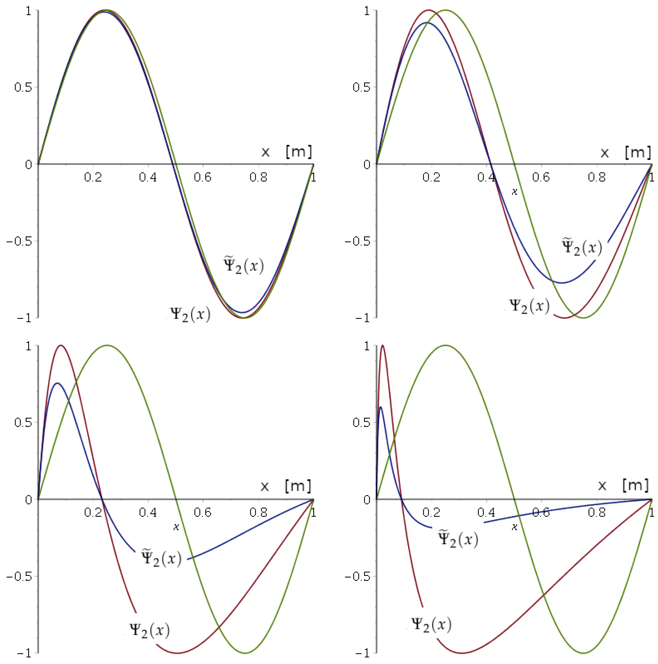
Ψ ˜ n ( x ) = A n sin n π ln ( 1 + α x ) ln ( 1 + α L ) 1 + α x n = 1 , 2 , 3
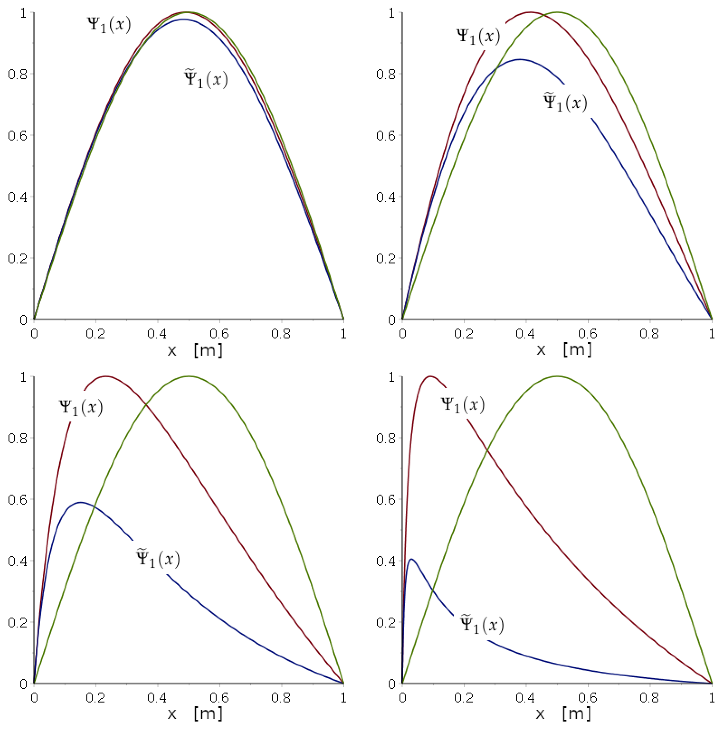
Figure 1 shows the different wave functions for the n = 1 case, with L = 1 and A 1 = 1 .
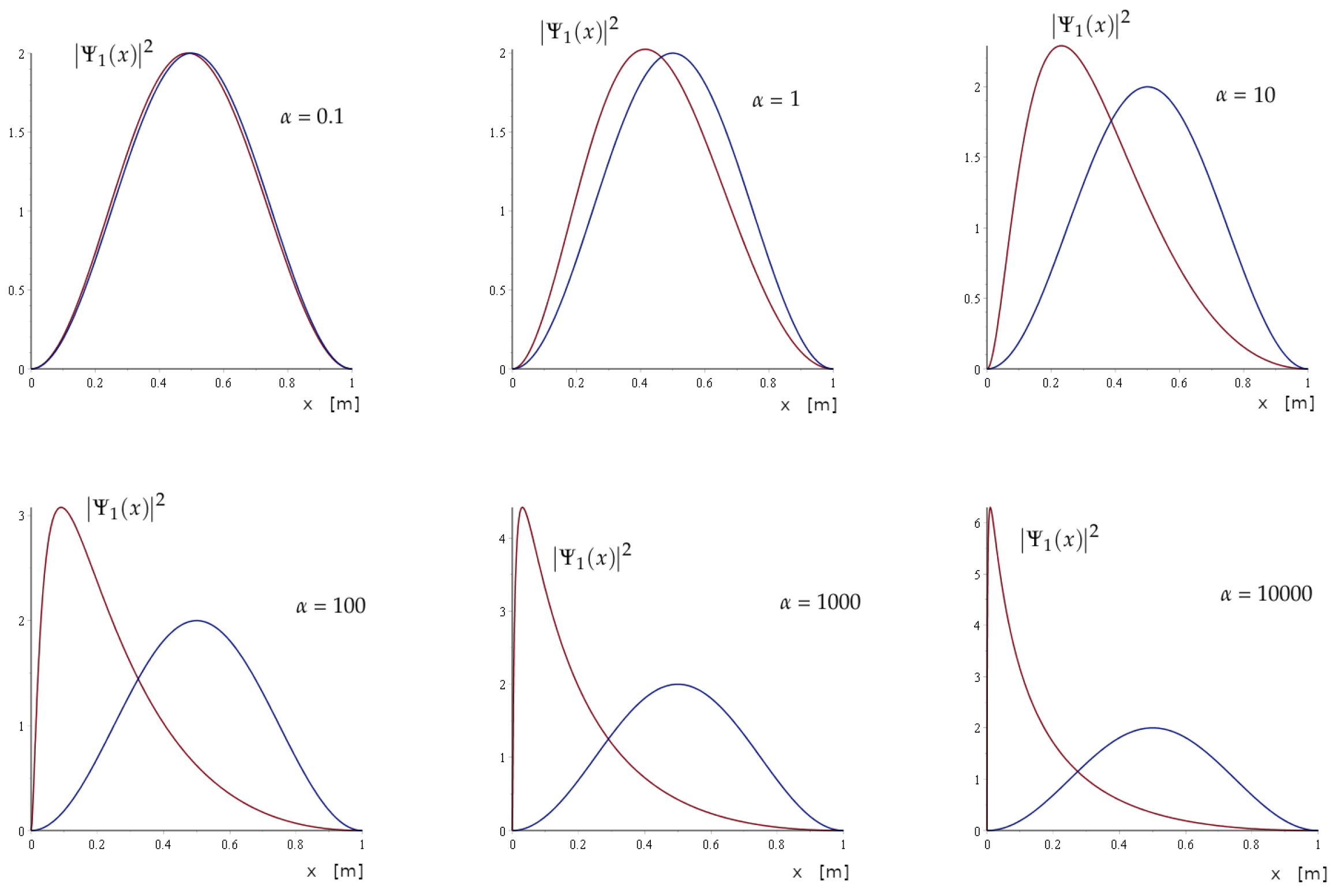
Figure 2 shows the probability density ρ ( x ) = | Ψ ( x ) | 2 of the deformed wave function Ψ 1 ( x ) with L = 1 .
Figure 3 shows the different wave functions for the n = 2 case, with L = 1 and A 2 = 1 .

2.7.5. The Hermiticity of p ^

In this case, consider the operator
p ^ = p ^ + K I
One has that
x ^ , p ^ = x ^ , p ^ + K I = x ^ , p ^ = i ( I + α x ^ )
Thus, p ^ satisfies the same deformed commutation relations (34). Thus, (34) does not determine p ^ in a unique way. There exists a whole operator family defined by (47) that satisfies the commutation relations (34). Now, from (40), one has that
p ^ = [ ( I + α x ^ ) p ^ 0 ] = [ p ^ 0 + α x ^ p ^ 0 ] = ( p ^ 0 + α p ^ 0 x ^ ) = p ^ 0 ( I + α x ^ ) p ^
Thus, the deformed momentum p ^ defined in (40) is not a Hermitian operator. In fact,
p ^ = p ^ i α I
However, the operator
p ^ = p ^ + p ^ 2 = p ^ + p ^ i α 2 = p ^ i α 2 I = i ( 1 + α x ) x i α 2
is a Hermitian operator and, due to the freedom given in (47), it also satisfies the deformed commutation relation (34). It is interesting to note that the complete algebra (42) remains invariant under the replacement p ^ p ^ .
From Equation (41), one observes that y ^ is a Hermitian operator because x ^ is Hermitian and α is real, and it is well defined for all values of x such that 1 + α x is not zero. Additionally, the complete algebra (42) remains invariant under the transformation given by
y ^ y ^ = y ^ + K ˜ I ,
where K ˜ is a constant. It is important to note that for y ^ to retain its Hermitian property, K ˜ must be a real number.

3. The Nonlinear p ^ Deformation Case

Finally, we consider the nonlinear momentum GUP
x ^ , p ^ = i g p ^
As is shown in [3], a deformed Heisenberg commutation relation of the above form can be represented by the differential operators
x ^ = x
p ^ = h p ^ 0
where the function h ( p ) is a solution to the differential equation [3]
d h ( p ) d p = g ( h ( p ) )

3.1. Classical Aspects

In the limit 0 , the quantum relation (51) goes to the classical one p = h p 0 . Thus, one can ask the following question: Does there exist, in this case, a canonical transformation between the deformed and non-deformed classical phase spaces? To answer this question, we state the following theorem:
Theorem 6. 
For the case of the GUP (50), the following transformation,
(53) p = p ( x , p 0 ) = h ( p 0 ) (54) y = y ( x , p 0 ) = x d h ( p 0 ) d p 0 ,
between the deformed ( y , p ) and non-deformed ( x , p 0 ) classical phase spaces is a canonical transformation.
Proof. 
Consider the following phase space transformation:
p = p ( x , p 0 ) = h ( p 0 )
y = y ( x , p 0 ) = χ ( x , p 0 )
for some χ function. Now, the Poisson bracket between the deformed phase space coordinates is
{ y , p } 0 = y x p p 0 p x y p 0 = χ ( x , p 0 ) x h ( p 0 ) p 0
and by imposing that { y , p } 0 = 1 , one obtains
χ ( x , p 0 ) x h ( p 0 ) p 0 = 1
The solution of this equation is
χ ( x , p 0 ) = x h ( p 0 ) + C ( p 0 )
where C ( p 0 ) is an arbitrary function of p 0 . Thus, there exists a whole family of transformations that satisfy (55). But if there is no deformation at all, then g ( p ) = 1 and (52) imply that
h ( p ) = p + C 1
with C 1 being a constant. To recover the correct limit p = p 0 in (53), the constant C ! must be zero, so h ( p ) = p . Similarly, one hopes also that for g ( p ) = 1 , the coordinate y becomes equal to x. To satisfy this boundary condition, the function C ( p 0 ) in (56) must vanish. Thus, finally, the classical canonical transformation associated with the deformed nonlinear Heisenberg relation (50) is
(57) p = p ( x , p 0 ) = h ( p 0 ) (58) y = y ( x , p 0 ) = x d h ( p 0 ) d p 0

3.2. Quantum Aspects

The quantum analogue of the above classical transformation is given by the following theorem:
Theorem 7. 
The quantum deformed operators defined by
(59) p ^ = h ( p ^ 0 ) (60) y ^ = x ^ h ( p ^ 0 ) 1
satisfy the standard Heisenberg algebra
[ y ^ , p ^ ] = i I
and also the GUP relation
[ x ^ , p ^ ] = i g ( p ^ )
Proof. 
First, consider
[ x ^ , p ^ ] = [ x ^ , h ( p ^ 0 ) ]
But standard manipulations imply that
[ x ^ , h ( p ^ 0 ) ] = i d h ( p ^ 0 ) d p 0 = i h ( p ^ 0 )
and Equation (52) gives
[ x ^ , h ( p ^ 0 ) ] = i g ( h ( p ^ 0 ) )
so
[ x ^ , p ^ ] = i g ( h ( p ^ 0 ) ) = i g ( p ^ )
Now,
[ y ^ , p ^ ] = [ x ^ h ( p ^ 0 ) 1 , h ( p ^ 0 ) ] = x ^ h ( p ^ 0 ) 1 h ( p ^ 0 ) h ( p ^ 0 ) x ^ h ( p ^ 0 ) 1 = [ x ^ , h ( p ^ 0 ) ] h ( p ^ 0 ) 1 = i h ( p ^ 0 ) h ( p ^ 0 ) 1 = i I

3.3. The Schrödinger Equation

We can write the Schrödinger equation in both phase spaces according to
Theorem 8. 
The Schrödinger equation in the non-deformed and deformed phase spaces is given, respectively, by the PDEs
1 2 m h i x 2 Ψ + U ( x ) Ψ = E Ψ
2 2 m 2 Ψ ( y ) y 2 + U y h ( h 1 ( i y ) ) Ψ ( y ) = E Ψ ( y )
Proof. 
In the non-deformed phase space ( x , p 0 ) , the quantization of the classical Hamiltonian function (23) by the representation (59) implies the Schrödinger equation
1 2 m h ( p ^ 0 ) 2 Ψ + U ( x ^ ) Ψ = E Ψ
And by (17), one gives
1 2 m h i x 2 Ψ + U ( x ) Ψ = E Ψ
To write the Schrödinger equation in the deformed phase space, one considers
p ^ 2 2 m Ψ + U ( x ^ ) Ψ = E Ψ
From (59) and (60), one can write x ^ in terms of y ^ and p ^ as
x ^ = y ^ h ( p ^ 0 ) = y ^ h ( h 1 ( p ^ ) )
so
p ^ 2 2 m Ψ + U ( y ^ h ( h 1 ( p ^ ) ) ) Ψ = E Ψ
Using the representation (45), the Schrödinger equation in the ( y , p ) space becomes
2 2 m 2 Ψ ( y ) y 2 + U y h ( h 1 ( i y ) ) Ψ ( y ) = E Ψ ( y )
Note that, depending on the h ( p ) function, Equation (61) can be of infinite order.

3.4. Example: The Linear p ^ Deformation Case

As an example of the momentum deformation case, consider now g ( p ) = 1 + β p .
The Heisenberg algebra is, then,
x ^ , p ^ = i I + β p ^
A representation of these commutation relations in terms of differential operators is given by
x ^ = x
p ^ = 1 β e β p ^ 0 I
where p ^ 0 = i x is the standard momentum operator for β = 0 . Note that, in this case, p ^ is Hermitian because p ^ 0 is Hermitian.
In the classical limit 0 , one has that p ^ p and p ^ 0 p 0 , so the classical version of (67) becomes
p = 1 β e β p 0 1
which gives a relation analogous to Equation (57). To obtain the corresponding relation for the y coordinate, that is, the equivalent to relation (58), we consider the transformation y = χ ( x , p ) and impose that { y , p } = 1 . Now,
{ y , p } = { y , p } 0 = y x p p 0 p x y p 0 = χ ( x , p 0 ) x e β p 0
so
χ ( x , p 0 ) x e β p 0 = 1
Then, by integrating this equation, one obtains
χ ( x , p 0 ) = x e β p 0
where the integration constant was chosen equal to zero to recover the proper limit y x for β 0 . Thus, the phase space transformation
(68) p = p ( x , p 0 ) = 1 β e β p 0 1 (69) y = y ( x , p 0 ) = x e β p 0
from non-deformed ( x , p 0 ) to the deformed ( y , p ) phase space is a canonical transformation.
The above transformation maps the whole phase space ( x , p 0 ) into the upper plane y > 1 β of the deformed phase space ( y , p ) . The classical theories will only be equivalent in these regions. It is important to note that to access the lower region y < 1 β , a complex momentum p 0 is required.
For the quantum version of this transformation, one would consider the operator transformation
(70) p ^ = 1 β e β p ^ 0 I (71) y ^ = x ^ e β p ^ 0
As a corollary of Theorem 7, one has that
[ y ^ , p ^ ] = i I
Thus, the operators p ^ and y ^ , defined by (70) and (71), are canonically conjugate at the quantum level.
Consider now the time-independent Schrödinger equation in the ( x , p 0 ) phase space. We start with the classical Hamiltonian function (23) and quantize this Hamiltonian by the rule (65). By using the representation (67), one has that
1 2 m β 2 e β p ^ 0 I 2 Ψ + U ( x ^ ) Ψ = E Ψ
To write this equation in the deformed ( y , p ) phase space, we need the inverses of Equations (70) and (71), which are
(74) p ^ 0 = 1 β ln I + β p ^ (75) x ^ = y ^ I + β p ^
Thus,
1 2 m p ^ 2 + U ( y ^ I + β p ^ ) Ψ = E Ψ
Now, by using the representation (45), one arrives at
2 2 m 2 Ψ ( y ) y 2 + U y 1 i β y Ψ ( y ) = E Ψ ( y )
Note that, in this case, the Schrödinger Equation (73) in the ( x , p 0 ) space is an infinite-order PDE, whereas in the ( y , p ) phase space, if the potential U = U ( x ) is a power of n, such as U ( x ) = x n , then the Schrödinger Equation (76) is an order n finite-dimensional PDE. But if U ( x ) admits a Taylor expansion as
U ( x ) = u 0 + u 1 x + u 2 x 2 +
then the Schrödinger Equation (76) also becomes of infinite order.
For example, in the free case U ( x ) = 0 , the infinite-dimensional Equation (73) in the ( x , p o ) phase-space is
1 2 m β 2 e β p ^ 0 I 2 Ψ = E Ψ
whose solutions are the eigenstates Φ of non-deformed momentum p ^ 0 ( p ^ 0 Φ = p 0 Φ ) and
E = E ( p 0 ) = 1 2 m β 2 e β p 0 1 2
Note that the spectrum in terms of p 0 is not symmetric, and this property has several physical consequences (for details, see [28]). Instead, Equation (76) for the free case is the finite-dimensional EDP
2 2 m 2 Ψ ( y ) y 2 = E Ψ ( y )
and its solution is just a standard plane-wave Ψ ( y ) = e i p y in the ( y , p ) phase-space (which is an eigenstate of the deformed momentum operator p ^ ). Also,
E = E ( p ) = p 2 2 m
is the standard quadratic relation between energy and momentum. Of course, due to the classical relation (68), both forms for the energy E ( p 0 ) and E ( p ) are equivalent.

3.5. Example: The Quadratic p ^ Deformation Case

As a second example of the momentum deformation case, consider g ( p ) = 1 + β p 2 .
The Heisenberg algebra is, then,
x ^ , p ^ = i I + β p ^ 2
The h function in (52) satisfies
d h ( p ) d p = 1 + β h ( p ) 2
with the solution [3,29]
h ( p ) = tan ( p β ) β
Thus, the Heisenberg algebra (77) can be represented by the differential operators
x ^ = x p ^ = tan β p ^ 0 β
The canonical transformation (53) of Theorem 4 is, then,
p = h ( p 0 ) = tan ( p 0 β ) β
y = x d h ( p 0 ) d p 0 = x cos 2 ( p 0 β )
Note that, in this case, the canonical transformation periodically maps the non-deformed momentum p 0 to the deformed phase space ( y , p ) . For example, the region
R = ( x , p 0 ) R 2 : < x < π 2 β p 0 π 2 β
is mapped to the whole plane ( y , p ) . Again, only in these specific regions will the classical and quantum theories be equivalent in both phase spaces.

4. The Harmonic Oscillator

In this section, we will analyze one of the most fundamental examples in physics: the harmonic oscillator. References such as [11,12,30,31,32,33] explore some quantum properties of this system under deformed Heisenberg commutation relations.
In this section, however, we will focus on examining the consequences of these generalized uncertainty principles (GUPs) on the classical evolution of the harmonic oscillator, specifically for the linear deformation cases discussed earlier.

4.1. Linear x ^ Deformation Case in the ( x , p 0 ) Phase Space

The classical Hamiltonian (23) for the harmonic oscillator has a potential energy U ( x ) = 1 2 k x 2 , where x represents the particle’s horizontal position, so
H = p 2 2 m + 1 2 k x 2
For the x linear deformed algebra (34), p and p 0 are related according to (57), so
H = H ( x , p 0 ) = ( 1 + α x ) 2 p 0 2 2 m + 1 2 k x 2
The Hamilton equations are, then,
p ˙ 0 = H x = α ( 1 + α x ) p 0 2 m k x
x ˙ = H p 0 = ( 1 + α x ) 2 p 0 m
By solving p 0 from (82) in terms of x ˙ and by replacing it in (81), one obtains the following differential equation for x:
x ¨ = α x ˙ 2 ( 1 + α x ) k m x ( 1 + α x ) 2
Note that apart from the elastic force term k x , a new effective force term α x ˙ 2 ( 1 + α x ) appears, as a residue of the deformed Heisenberg algebra (34) at the classical level. For α 0 , one recovers the usual harmonic oscillator equation of motion.
The solutions of Equation (83) are
x 1 ( t ) = 4 C 1 α m 2 e C 1 α 2 m k m C 2 + t 4 C 1 k m 3 e C 1 α 2 m k m C 2 + t 2 4 C 1 α k m 3 + α e C 1 α 2 m k m C 2 + t 2 4 k m e C 1 α 2 m k m C 2 + t
and
x 2 ( t ) = 4 C 1 α m 2 e C 1 α 2 m k m C 2 + t 4 C 1 k m 3 e C 1 α 2 m k m C 2 + t 2 4 C 1 α k m 3 + α e C 1 α 2 m k m C 2 + t 2 4 k m e C 1 α 2 m k m C 2 + t
where C 1 and C 2 are arbitrary constants. The corresponding solution for the momentum is
p 0 ( t ) = d d t x ( t ) m α 2 x ( t ) 2 + 2 α x ( t ) + 1
Thus, one can see that the solutions will be oscillatory only if
C 1 α 2 < k m ,
and under this condition, the motion period becomes
T = 2 π m | C 1 α 2 m k |
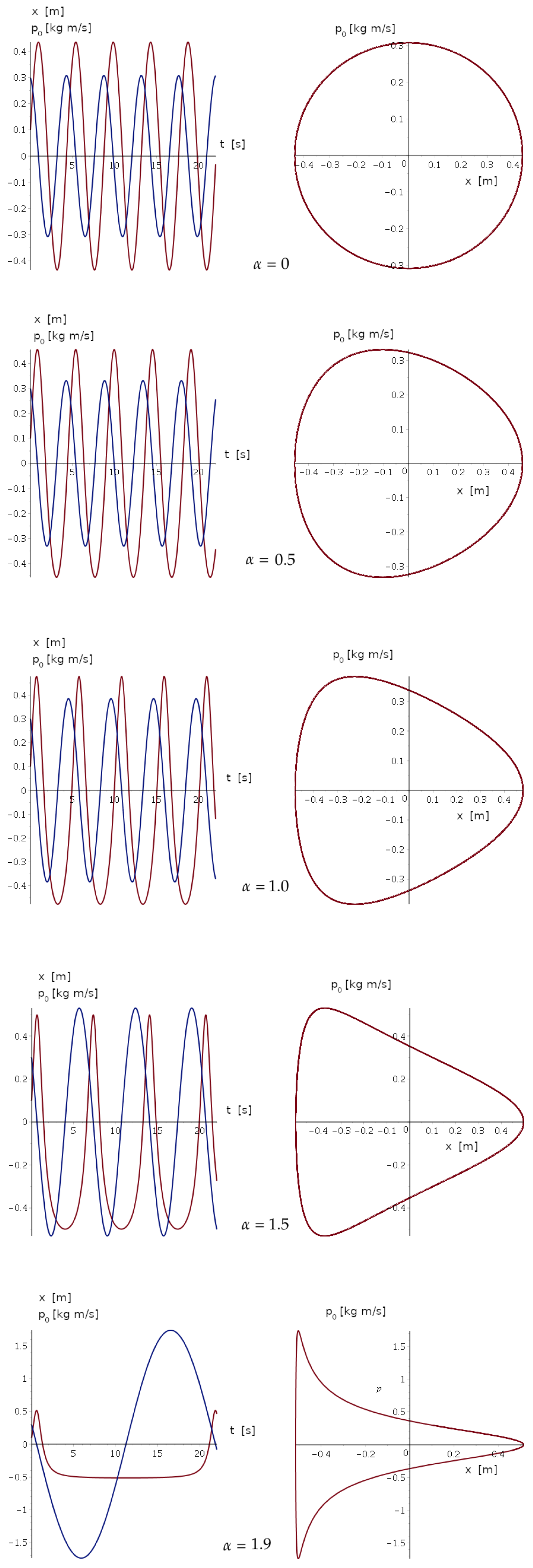
It is important to note that, unlike the non-deformed harmonic oscillator, the period in this case explicitly depends on the initial conditions. Consequently, for a specific deformation parameter α value and particular initial conditions in phase space, the period displays resonance when C 1 α 2 = k m . Figure 4 shows, in the left column, the solution x ( t ) (red curve) and p 0 ( t ) (blue curve) of the Hamiltonian equations of motion (81) and (82). The right column shows the phase space diagram for different α values.

4.2. Linear x ^ Deformation Case in the ( y , p ) Phase Space

By using the inverse transformation (43), one can write the Hamiltonian (80) in the ( y , p ) phase space as follows:
H ( y , p ) = p 2 2 m + k 2 α 2 e α y 1 2
The Hamiltonian equations now read as follows:
p ˙ = H y = k α e α y 1 e α y
y ˙ = H p = p m
By solving p from (85) in terms of y ˙ , and by replacing it in (84), one obtains the following differential equation for y:
y ¨ = k m α e α y 1 e α y
By replacing transformations (57) and (58) in the Hamiltonian Equations (84) and (85), one obtains the same Hamiltonian system (81) and (82).

4.3. Linear p ^ Deformation Case in the ( x , p 0 ) Phase Space

In the case of the p ^ linear deformed algebra (65), the classical variables p and p 0 are related according to (68), so
H = H ( x , p 0 ) = e β p 0 1 2 2 m β 2 + 1 2 k x 2
The Hamilton equations are
p ˙ 0 = H x = k x
x ˙ = H p 0 = e β p 0 1 e β p 0 m β
In this case, by solving x from (87) and replacing in (88), one obtains
p ¨ 0 = k e β p 0 1 e β p 0 m β
Note that Equations (88) and (89) can be mapped to the β = 1 case by performing a scaling transformation p 0 p 0 = β p 0 and x x = β x . That is, if x and p 0 satisfy
x ˙ = e p 0 1 e p 0 m
p ¨ 0 = k e p 0 1 e p 0 m ,
then the solution for β 1 can be obtained as x ( t ) = x ( t ) β and p 0 ( t ) = p 0 ( t ) β .
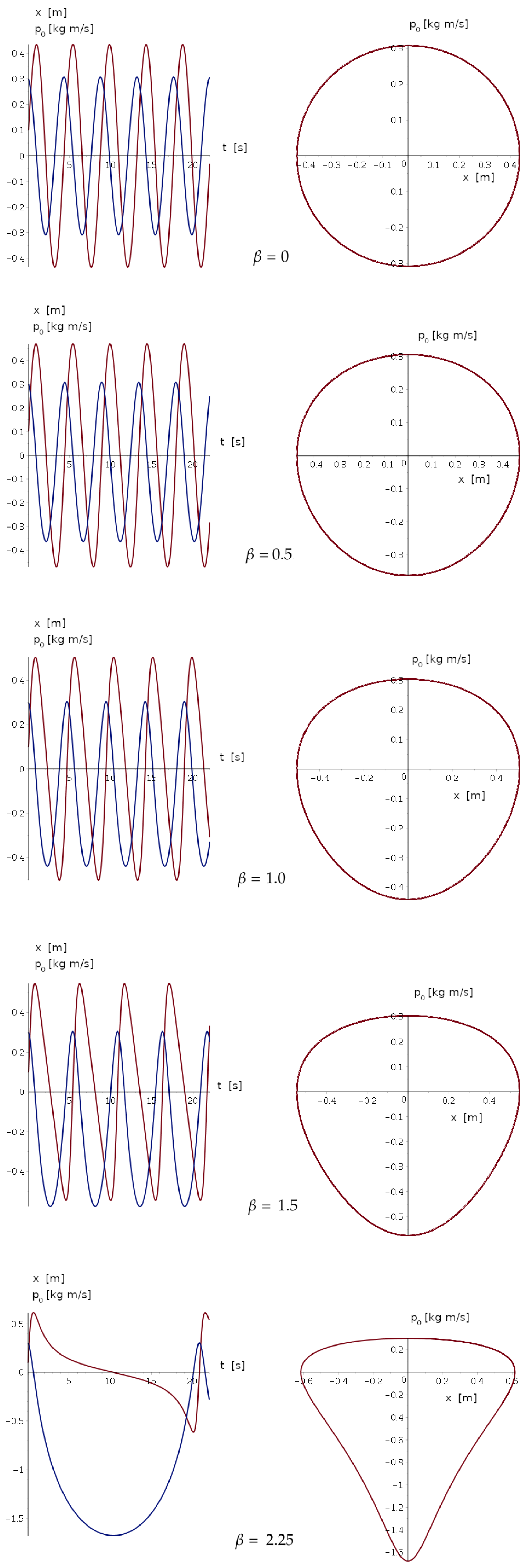
Figure 5 shows, in the left column, the solution x ( t ) (red curve) and p 0 ( t ) (blue curve) of the Hamiltonian equations of motion (87) and (88). The right column shows the phase space ( x , p 0 ) diagram for different β values. In this case, we do not have explicit solutions to the motion’s equations. However, the numerical analysis shown in Figure 5 indicates that the motion’s period exhibits a similar resonant behavior to that observed in the x-deformation case studied previously.

4.4. Linear p ^ Deformation Case in the ( y , p ) Phase Space

Using the inverse of the transformation transformation (68) and (69), that is,
x = y ( 1 + β p )
p 0 = 1 β ln 1 + β p
the Hamiltonian (86) can be written as in the ( y , p ) phase space as follows:
H = H ( y , p ) = p 2 2 m + 1 2 k 1 + β p 2
The corresponding Hamiltonian equations are
p ˙ = H y = k y 1 + β p 2
y ˙ = H p = p m + k β y 2 1 + β p
Now, by again using the transformation (68) and (69) and replacing them in the Hamiltonian equations above, one obtains the same system (87) and (88).

5. Conclusions

This paper examines the meaning of the modified canonical Heisenberg commutation relations from a standard Hamiltonian perspective. The following questions were analyzed: What does a relation of this type mean in Hamiltonian theory? What are the canonical variables in this model? The answer stems from the existence of two different phase spaces. The first, called the non-deformed phase (obtained for the deformation control parameter value equal to zero), is defined by the Cartesian x ^ coordinate operator and its non-deformed conjugate momentum p ^ 0 operator, which satisfies the standard quantum mechanical Heisenberg commutation relation. The second phase space, the deformed one, is given the deformed momentum operator p ^ and a new position y ^ operator, which also satisfies the canonical commutation relation.
At the classical level, we found a classical canonical transformation that maps the non-deformed phase space into the deformed one for a specific class of deformation algebras. Also, from a quantum mechanical point of view, an operator transformation between these same phase spaces is given, which permits a Schrödinger equation to be written in both spaces, so there are two equivalent quantum mechanical descriptions associated with a deformed commutation relation.
Additionally, we explored, at the classical level, the consequences of the deformed Heisenberg commutation relation on a well-known system: the harmonic oscillator. In particular, we studied the deformation of the classical Hamiltonian equation of motion by incrementing the deformation parameter for the linear deformation in the position and momentum. In all cases, the phase space diagrams started to differ from the usual one as the deformation parameter increased. Also, the motion period, unlike the non-deformed harmonic oscillator, explicitly depends on the initial conditions, and an interesting resonance phenomenon occurs: for a specific deformation parameter value and particular initial conditions in phase space, the period diverges.
Finally, we would like to emphasize that generalized uncertainty principles (GUPs) are extensions of standard quantum mechanics. Our objective is to offer a standard Hamiltonian interpretation of these generalized commutation relations. Such interpretations are part of a broader and well-established tradition of operator-based formulations of mechanics in phase space.
A noteworthy example in this context is the Koopman–von Neumann (KvN) formalism, which introduces a Hilbert space representation for classical mechanics. The KvN theory originated in the 1930s through the work of Koopman [34], who noted that the phase space of a classical system can be transformed into a Hilbert space. This model was further developed by John von Neumann [35] and Denys I. Bondar [36], and it relies on the self-adjoint Liouvillian operator [37]
L ^ = i H ( x , p ) p x + i H ( x , p ) x p
where H ( x , p ) denotes the classical Hamiltonian, and this theory postulated that the KvN wave function ψ ( x , p , t ) satisfies the equation
i t ψ ( x , p , t ) = L ^ ψ ( x , p , t ) ,
which has the same form as the Liouville equation of classical statistical mechanics. For our discussion, it is essential to note that the KvN theory satisfies the Ehrenfest theorems
d d t x = p m d d t p = V ( x )
under a pure classical, non-commutative framework. To accomplish that, the Liouvillian operator L ^ must be constructed not only from the usual momentum p ^ and position x ^ operators, but also from two additional operators, θ ^ and λ ^ . These operators must adhere to specific commutation relations [37,38] given by
[ x ^ , θ ^ ] = [ p ^ , λ ^ ] = i
x ^ , p ^ = [ x ^ , λ ^ ] = [ p ^ , θ ^ ] = 0
[ θ ^ , λ ^ ] = 0 ,
which is known as the Koopman–von Neumann algebra, and L ^ becomes
L ^ = L ( x ^ , p ^ , θ ^ , λ ^ ) = p ^ θ ^ m V ( x ^ ) λ ^ + C ( x ^ , p ^ ) ,
which is the called the Koopman generator of KvN theory. From the point of view developed in this article, the commutations relations (94) show that θ ^ and λ ^ can be thought of as canonical variables conjugate to the position x ^ and the “deformed” momentum p ^ , respectively, for = 1 , which defines two different phase spaces naturally. The difference is that for the GUP case, the commutator (95) is different from zero (e.g., see Equation (22)). Note that from our perspective, L ^ in (96) is a hybrid object.
In summary, the Koopman–von Neumann theory maps standard classical mechanics, wherein observables commute, onto an operator formalism governed by a hybrid Liouvillian. In contrast, the present work instead maps a non-standard quantum algebra onto a standard quantum algebra.
Another operator-based formulation of quantum mechanics in phase space is deformation quantization, which is related to non-commutative quantum mechanics. The idea here is to introduce phase space quantization as a deformation of the classical theory. Deformation quantization depends on the Groenewold–Moyal product M , which is defined for two phase space functions, f ( x , p ) and g ( x , p ) , according to
f M g ( q , p ) = f q + i 2 p , p i 2 q g ( q , p )
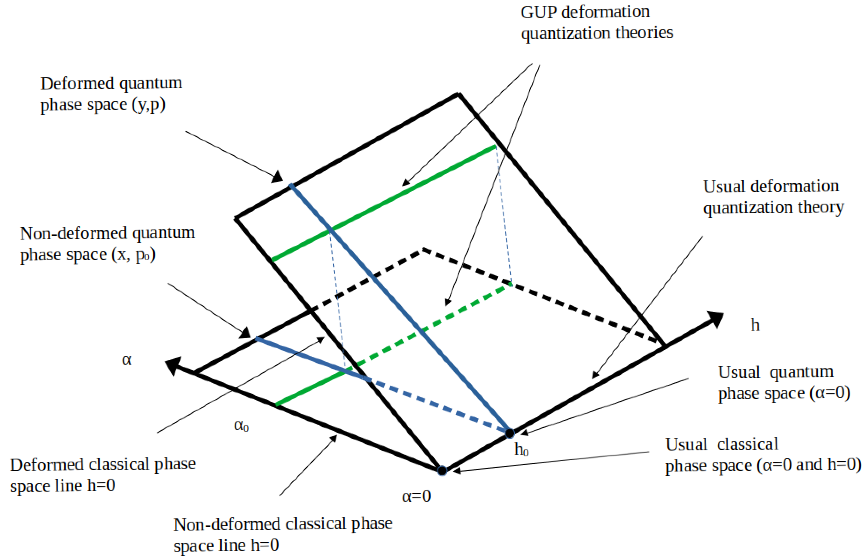
and includes a Taylor expansion at all orders in . In some sense, the deformation is along the Planck constant axis. The GUP relations studied in this paper, in contrast, are only of linear order in . However, GUP deformation (measured, for example, by the α constant in (34)) can be thought of as running along an α axis that is “orthogonal” to the axis. Figure 6 below illustrates this idea.
Note that deformation quantization is defined along the α = 0 axis only, and includes contributions along all orders in h along the h axis. GUP deformation instead runs along the orthogonal α axis, and for any α 0 and h 0 , there are two different phase spaces: the deformed phase space ( y , p ) (given by the upper inclined plane) and the non-deformed phase space ( x , p 0 ) (given by the horizontal plane). The associated classical theories (for h = 0 ) are given by the left extreme lines along these planes. Note that for α = 0 , both phase spaces coincide (h axis).
For some h 0 , as per h 0 in Figure 6, the blue lines along the inclined and horizontal planes represent, respectively, the deformed and non-deformed quantum phase spaces of the theory for that fixed h 0 value. From the figure, one hopes that for α 0 there exists a deformed Groenewold–Moyal product M α that runs along the h axis. In fact, there would exist two such Groenewold–Moyal products: one M α d for the deformed phase space (green line at the upper plane) and a M α n d for the non-deformed phase space (green line at the lower plane). Moreover, such Groenewold–Moyal products would be related to some one-to-one transformation, because these phase spaces are equivalent. In a forthcoming paper, we address these issues in detail.


Author Contributions

Conceptualization, M.C.G., R.O.H. and J.M.G.; methodology, M.C.G., R.O.H. and J.M.G.; formal analysis, M.C.G. and J.M.G.; investigation, M.C.G. and R.O.H.; writing—original draft, M.C.G.; writing—review and editing, M.C.G., R.O.H. and J.M.G. All authors have read and agreed to the published version of the manuscript.

Funding

This research received no external funding.

Data Availability Statement

No new data were created or analyzed in this study. Data sharing is not applicable to this article.

Conflicts of Interest

The authors declare no conflicts of interest.

References

  1. Tawfik, A.N.; Diab, A.M. A review of the generalized uncertainty principle. Rep. Prog. Phys. 2015, 78, 126001. [Google Scholar] [CrossRef] [PubMed]
  2. Bruneton, J.P.; Larena, J. Quantum theory of the generalised uncertainty principle. Gen. Relativ. Gravit. 2017, 49, 56. [Google Scholar] [CrossRef]
  3. Pedram, P. A class of GUP solutions in deformed quantum mechanics. Int. J. Mod. Phys. D 2010, 19, 2003–2009. [Google Scholar] [CrossRef]
  4. Seifi, M.; Sefiedgar, A.S. The effects of the covariant generalized uncertainty principle on quantum mechanics. Can. J. Phys. 2022, 101, 242–247. [Google Scholar] [CrossRef]
  5. Luciano, G.G.; Petruzziello, L. Generalized uncertainty principle and its implications on geometric phases in quantum mechanics. Eur. Phys. J. Plus 2021, 136, 179. [Google Scholar] [CrossRef]
  6. Scardigli, F. The deformation parameter of the generalized uncertainty principle. J. Phys. Conf. Ser. 2019, 1275, 012004. [Google Scholar] [CrossRef]
  7. Casadio, R.; Scardigli, F. Generalized Uncertainty Principle, Classical Mechanics, and General Relativity. Phys. Lett. B 2020, 807, 135558. [Google Scholar] [CrossRef]
  8. Chester, D.; Arsiwalla, X.D.; Kauffman, L.H.; Planat, M.; Irwin, K. Quantization of a New Canonical, Covariant, and Symplectic Hamiltonian Density. Symmetry 2024, 16, 316. [Google Scholar] [CrossRef]
  9. Cremaschini, C.; Tessarotto, M. Planck Length Emerging as the Invariant Quantum Minimum Effective Length Determined by the Heisenberg Uncertainty Principle in Manifestly Covariant Quantum Gravity Theory. Symmetry 2024, 16, 1042. [Google Scholar] [CrossRef]
  10. Contreras González, M.; Villena, M.; Ortiz Herrera, R. An Optimal Control Perspective on Classical and Quantum Physical Systems. Symmetry 2023, 15, 2033. [Google Scholar] [CrossRef]
  11. Kempf, A.; Mangano, G.; Mann, R.B. Hilbert space representation of the minimal length uncertainty relation. Phys. Rev. D 1995, 52, 1108. [Google Scholar] [CrossRef] [PubMed]
  12. Bagchi, B.; Fring, A. Minimal length in quantum mechanics and non-Hermitian Hamiltonian systems. Phys. Lett. A 2009, 373, 4307–4310. [Google Scholar] [CrossRef]
  13. Bruno, M.; Segreto, S.; Montani, G. Generalized uncertainty principle theories and their classical interpretation. Nucl. Phys. B 2024, 1009, 116739. [Google Scholar] [CrossRef]
  14. Reginatto, M.; Hall, M.J.W. Entangling quantum fields via a classical gravitational interaction. J. Phys. Conf. Ser. 2019, 1275, 012039. [Google Scholar] [CrossRef]
  15. Övgün, A. Entangled Particles Tunneling From a Schwarzschild Black Hole immersed in an Electromagnetic Universe with GUP. Int. J. Theor. Phys. 2016, 55, 2919–2927. [Google Scholar] [CrossRef]
  16. Park, D. Quantum entanglement with generalized uncertainty principle. Nucl. Phys. B 2022, 977, 115736. [Google Scholar] [CrossRef]
  17. Guo, X.; Wang, P.; Yang, H. The classical limit of minimal length uncertainty relation: Revisit with the Hamilton-Jacobi method. J. Cosmol. Astropart. Phys. 2016 5, 062. [CrossRef]
  18. Reginatto, M. Exact Uncertainty Principle and Quantization: Implications for the Gravitational Field. Braz. J. Phys. 2005, 35, 476–480. [Google Scholar] [CrossRef][Green Version]
  19. Szalowski, K. Phase Diagram and Quantum Entanglement Properties of a Pentamer S = 1/2 Heisenberg Spin Cluster. Molecules 2023, 28, 6418. [Google Scholar] [CrossRef]
  20. Gonçalves, A.O.O.; Gusson, M.F.; Dilem, B.B.; Furtado, R.G.; Francisco, R.O.; Fabris, J.C.; Nogueira, J.A. An infinite square-well potential as a limiting case of a square-well potential in a minimal-length scenario. Int. J. Mod. Phys. A 2020, 35, 2050069. [Google Scholar] [CrossRef]
  21. Rojo, A.G.; Berman, P.R. The infinite square well potential in momentum space. Eur. J. Phys. 2020, 41, 055404. [Google Scholar] [CrossRef]
  22. Chung, W.S.; Hassanabadi, H. A new higher order GUP: One dimensional quantum system. Eur. Phys. J. C 2019, 79, 213. [Google Scholar] [CrossRef]
  23. Blado, G.; Owens, C.; Meyers, V. Quantum wells and the generalized uncertainty principle. Eur. J. Phys. 2014, 35, 065011. [Google Scholar] [CrossRef][Green Version]
  24. Blado, G.; Prescott, T.; Jennings, J.; Ceyanes, J.; Sepulveda, R. Effects of the generalised uncertainty principle on quantum tunnelling. Eur. J. Phys. 2016, 37, 025401. [Google Scholar] [CrossRef]
  25. Bernardo, R.C.S.; Esguerra, J.P. Energy levels of one-dimensional systems satisfying the minimal length uncertainty relation. Ann. Phys. 2016, 373, 521–531. [Google Scholar] [CrossRef]
  26. Shababi, H.; Pedram, P.; Chung, W.S. On the quantum mechanical solutions with minimal length uncertainty. Int. J. Mod. Phys. A 2016, 31, 1650101. [Google Scholar] [CrossRef]
  27. Das, S.; Vagenas, E.C. Phenomenological implications of the generalized uncertainty principle. Can. J. Phys. 2009, 87, 3. [Google Scholar] [CrossRef]
  28. Contreras, M.; Ortiz, R.; González, M. Modified Heisenberg commutation relations and the infinite-square well potential: Some simple consequences. Symmetry 2024, 16, 1268. [Google Scholar] [CrossRef]
  29. Contreras, M.; Ortiz, R.; González, M. Modified Heisenberg commutation relations, free Schrödinger equations, tunnel effect and its connections with the Black-Scholes equation. Axioms 2025, 14, 60. [Google Scholar] [CrossRef]
  30. Naimi, Y. A Class of Solutions under GUP for a Harmonic Oscillator and a Particle in a Box. Gravit. Cosmol. 2016, 22, 382–387. [Google Scholar] [CrossRef]
  31. Mu, B.; Yu, R.; Wang, D. Spectra of Harmonic Oscillators with GUP and Extra Dimensions. J. High Energy Phys. Gravit. Cosmol. 2019, 5, 279–290. [Google Scholar] [CrossRef][Green Version]
  32. Ramezani, H.; Nozari, K. Linear–quadratic GUP and thermodynamic dimensional reduction. Ann. Phys. 2024, 469, 169752. [Google Scholar] [CrossRef]
  33. Bosso, P.; Das, S.; Mann, R. Planck scale corrections to the harmonic oscillator, coherent, and squeezed states. Phys. Rev. D 2017, 96, 066008. [Google Scholar] [CrossRef]
  34. Koopman, B.O. Hamiltonian Systems and Transformation in Hilbert Space. Proc. Natl. Acad. Sci. USA 1931, 17, 315–318. [Google Scholar] [CrossRef] [PubMed]
  35. von Neumann, J. Zur operatorenmethode in der Klassi sehen Mechanik. Ann. Math 1932, 33, 587. [Google Scholar] [CrossRef]
  36. Bondar, D.I.; Cabrera, R.; Lompay, R.R.; Ivanov, M.Y. Operational Dynamic Modeling Transcending Quantum and Classical Mechanics. Phys. Rev. Lett. 2012, 109, 190403. [Google Scholar] [CrossRef]
  37. Piasecki, D.W. Introduction to Koopman-von Neumann mechanics. arXiv 2021, arXiv:2112.05619. [Google Scholar] [CrossRef]
  38. Mauro, D. Topics in Koopman-von Neumann Theory. arXiv 2002, arXiv:quant-ph/0301172. [Google Scholar] [CrossRef]
Figure 1. The wave function Ψ 1 ( x ) (red curve) and the effective wave function Ψ ˜ 1 ( x ) (blue curve) for different α values. From left to right and from top to bottom: α = 0.1, 1, 10, 100. The green curve represents the non-deformed wave function for the case α = 0 .
Mathematics 13 03872 g001
Figure 2. Probability density ρ ( x ) = | Ψ ( x ) | 2 of the deformed wave function Ψ 1 ( x ) (red curve) and non-deformed wave function for the case α = 0 (blue curve), for different α values. From left to right and from top to bottom: α = 0.1 , 1 , 10 , 100 , 1000 , 10,000 .
Mathematics 13 03872 g002
Figure 3. The wave function Ψ 2 ( x ) (red curve) and the effective wave function Ψ ˜ 2 ( x ) (blue curve) for different α values. From left to right and from top to bottom: α = 0.1, 1, 10, 100. The green curve represents the non-deformed wave function for the case α = 0 .
Mathematics 13 03872 g003
Figure 4. Left column: The solution x ( t ) (red curve) and p 0 ( t ) (blue curve) of the Hamiltonian equations. Right column: The corresponding phase space ( x , p 0 ) diagram for different α values. From top to the bottom: α = 0, 0.5, 1.0, 1.5, 1.9. Here, m = 0.5 (kg), k = 1 (N/m), and the initial conditions are x ( 0 ) = 0.1 (m), p 0 ( 0 ) = 0.3 (kg m/s). Note that the period increases when C 1 α 2 k m .
Mathematics 13 03872 g004
Figure 5. Left column: The solution x ( t ) (red curve) and p 0 ( t ) (blue curve) of the Hamiltonian Equations (87) and (88). Right column: The corresponding phase space diagram ( x , p 0 ) for different β values. From top to the bottom: β = 0, 0.5, 1.0, 1.5, 2.25. Here, m = 0.5 (kg), k = 1 (N/m), and the initial conditions are x ( 0 ) = 0.1 (m), p 0 ( 0 ) = 0.3 (kg m/s). Note that as β increases, the period of motion increases gradually, approaching the resonance value in a similar way to the x-deformation case.
Mathematics 13 03872 g005
Figure 6. Deformed and non-deformed phase spaces representation.
Mathematics 13 03872 g006
Disclaimer/Publisher’s Note: The statements, opinions and data contained in all publications are solely those of the individual author(s) and contributor(s) and not of MDPI and/or the editor(s). MDPI and/or the editor(s) disclaim responsibility for any injury to people or property resulting from any ideas, methods, instructions or products referred to in the content.