Abstract
This manuscript introduces a generalized Markov Decision Process (MDP) model for dynamic capacity planning in the presence of stochastic time-nonhomogeneous demand, wherein system capacity may be flexibly increased or decreased throughout a finite planning horizon. The model includes investment, disinvestment, maintenance, operational, and shortage costs, in addition to a salvage value at the end of the planning horizon. Under very realistic conditions, we investigate the structural properties of the optimal policy and demonstrate its monotonic structure. By leveraging these properties, we propose a revised value iteration algorithm that capitalizes on the intrinsic structure of the problem, thereby achieving enhanced computational efficiency compared to traditional dynamic programming techniques. The proposed model is applicable across a range of sectors, including manufacturing systems, cloud-computing services, logistics systems, healthcare resource management, power capacity planning, and other intelligent infrastructures driven by Industry 4.0.
Keywords:
capacity planning; decision making under uncertainty; structured optimal policy; revised value iteration algorithm MSC:
90C40; 90B30
1. Introduction
The discipline of capacity planning is distinguished by a substantial body of academic research, encompassing a wide array of application domains, including (a) power generation and distribution; (b) production and supply chain logistics; (c) network systems such as electricity, radio, and mobile communications; and (d) hospital capacity planning. For an overview of this topic, the reader is referred to Ref. [1] along with the review articles listed therein.
There exists a broad array of modelling and solution methodologies for capacity planning, illustrating the heterogeneity and complexity inherent in real-world scenarios. This includes, but is not limited to, the following.
A diverse array of modelling techniques are currently used for capacity planning, including (a) mathematical programming techniques [2], (b) stochastic and dynamic programming methods [3,4], (c) robust optimization [5], and (d) simulation-based optimization [6,7]. With the exception of stochastic dynamic programming methods, these techniques are normally applied to deterministic problems or employed in policy evaluation. The challenge of sequential decision-making under stochastic demand conditions is most effectively modelled via stochastic dynamic programming. AlDurgam et al. [1] confirmed that the topic of sequential decision-making under conditions of uncertainty is considerably underrepresented in the literature in comparison to the aforementioned methodologies. A Markov decision process (MDP) is a discrete stochastic dynamic programming technique that is extensively employed to model sequential decision-making under uncertainty scenarios frequently observed in capacity planning. The assumption of static demand can result in significant ramifications, including, as thoroughly documented, instances of capacity shortages or excess capacities [8].
Characterising the optimal policies in MDPs facilitates the practical application of intricate models by resulting in simple decision rules [9], such as threshold or monotone policies, which can be easily executed by decision makers. Furthermore, these characteristics reduce the computational complexity of MDPs by limiting the solution space [10,11]. Recently Krishnamurthy [12] demonstrated that in Markov decision processes, optimal policies increase with the state under broader conditions than supermodularity, such as sigmoidal rewards and non-supermodular transitions. Their research confirmed monotonicity with totally positive order-three transition matrices and concave value functions. Lee et al. [13] analysed monotone policy iteration in Markov decision processes, offering convergence and optimality conditions and a modified policy iteration algorithm. They assessed nineteen state-ordering rules’ effects, finding a time–quality trade-off: faster orderings excel in structured scenarios, while random orderings reduce the optimality gap with more of a computational cost.
Martínez-Costa et al. [14] observed that strategic capacity-planning models generally emphasize expansion while paying less attention to capacity reduction—a gap that is particularly salient in global markets with rapid product cycles. In practice, workforce and logistics planning require the ability to scale resources both up and down. This pattern extends to the MDP literature: several studies (Table 1) formulate capacity planning as an MDP and concentrate on expansion under uncertainty, and apart from application cases, few provide rigorous structural characterizations of the optimal policies. Wu and Chuang [15] studied a multigeneration capacity portfolio expansion model involving uncertainties in price, demand, and lifecycle; established a monotone expansion policy; and formulated a revised value iteration algorithm. Wu and Chuang [11] further extended their study to encompass multi-type (flexible versus dedicated) capacity with uncertainties in demand, price, and yield, utilising the structural properties in their previous work [15], and proposed a heuristic search algorithm that improves computational efficiency by approximately 30%. Lin et al. [16] explored expansion and allocation across multiple sites under Markovian demand within a finite-horizon dynamic programming framework embedded into linear programming, although no structural properties were delineated. Mishra et al. [17] investigated a two-period product line expansion/reduction problem characterized by price-dependent stochastic demand, resulting in a news-vendor-like optimal policy in quantile form along with an analytical solution. Serrato et al. [18] modelled the outsourcing of reverse-logistics capacity over a finite horizon with binomial returns and demonstrated a threshold policy through a backward induction algorithm.

Table 1.
Summary of the most relevant MDB-based research articles.
Classically, Lindley recursions are associated with inventory and queueing models, yet the same reflected-random-walk dynamics govern capacity headroom under stochastic demand with discrete expand/contract actions. We therefore draw on three inventory studies as methodological antecedents. Recent research by Blancas-Rivera et al. [20] elucidates the conditions under which (s, S) policies are optimal, even in the presence of potentially unbounded costs. Their findings demonstrate that a subsequence of value-iteration minimizers converges to an optimal policy, substantiated through a numerical example. In the realm of periodic-review lost-sales models with positive lead times, van Jaarsveld and Arts [21] proposed the projected inventory-level (PIL) policy. This policy aims to maintain a fixed expected on-hand inventory upon arrival, and it has been analytically proven to dominate constant-order policies. The PIL policy achieves asymptotic optimality as the penalty for lost sales approaches infinity and, in scenarios with exponential demand, as the lead time becomes infinitely long. Their study also reports robust numerical performance. In a related investigation, Yuan et al. [22] establish that within lost-sales systems characterized by stochastic lead times, base-stock policies attain asymptotic optimality when the penalty for lost sales significantly surpasses holding costs, with the incurred costs converging to the system’s optimum.
The studies most pertinent to this research are those conducted by references [17,18]. Serrato et al. [18] investigated outsourcing decisions constrained to expansion scenarios under the assumption of binomially distributed returns. Conversely, Mishra et al. explored a two-period model characterized by demand contingent on price, which resulted in an analytical solution comparable to the newsvendor model. Distinctively, our model extends the model developed by Abduljaleel and AlDurgam [19] to accommodate both expansion and reduction decisions. We incorporate a general stochastic demand model that allows for time-nonhomogeneous demands and derive a monotone structure under realistic cost conditions. Utilising these characteristics, we have developed a revised value iteration algorithm that significantly diminishes computational effort in comparison to the conventional backward value iteration method.
The remainder of this paper is structured as follows. Section 2 provides a formal definition and MDP formulation of the problem at hand. Section 3 presents the structural properties of the model and their advantages with respect to computational efficiency. Based on the structural properties of the MDP model, a modified value iteration algorithm is given in Section 4, and illustrative numerical examples are presented in Section 5. Section 6 concludes the paper.
2. Problem Definition and MDP Model
In this section, we provide the problem definition, notations, and MDP model of the problem at hand.
2.1. Problem Definition
This study addresses a problem of multi-period capacity planning wherein a decision maker is tasked with meeting stochastic dynamic demands. The model assumes there is a Markovian demand process [23]; that is, the probability distribution of the demand in the next time period depends only on the demand realised in the current period. In any time period, the system’s capacity represents the maximum demand it can satisfy internally in that period. Any demand exceeding this capacity incurs a penalty due to emergency processing or expediting. In every time-period, there will be a maintenance cost for maintaining the overall system capacity and an operating cost for the utilised system capacity. At the end of each period, the decision maker decides how much to increase or decrease the system capacity. There is no backordering of demand; that is, at any point in time, if the demand is not met by the system’s capacity, it is processed externally, incurring a penalty cost. The optimal decision policy defines the optimal action in every time period for each possible system state, with the objective of minimising overall system costs over the entire planning horizon.
2.2. Nomenclature
Next, the notations used to construct the MDP model are provided.
denotes the action taken at time when the system is in state . For simplicity, is used interchangeably with . Positive values represent increasing the capacity of the system, and negative values represent decreasing the capacity of the system.
denotes the optimal action taken at time when the system is in state . For simplicity, is used interchangeably with
denotes action space at time when the system is in state . For simplicity, is used interchangeably with
denotes the cost of increasing the capacity of the system by one unit; this represents an investment cost ($ per unit of capacity).
denotes the cost of decreasing the capacity of the system by one unit; this represents disinvestment cost/reward ($ per unit of capacity). can take negative values to represent rewards.
denotes capacity maintenance cost ($ per unit of capacity available per time period).
denotes operating cost. This represents the cost incurred in meeting a unit of demand by the existing system capacity ($ per unit of capacity demanded per time period).
denotes shortage cost or the penalty incurred per unit of demand exceeding current system capacity ($ per unit short of capacity per time period).
denotes the cost of salvaging a unit of capacity of the system at the end of the planning horizon, , ($ per unit of capacity). To represent rewards, can take negative values.
denotes System capacity at time (units of capacity).
denotes demand for units of capacity at time (units of capacity).
denotes the maximum possible capacity available for the decision maker at any point in time.
denotes the conditional probability the state at time will be , given that the state and action taken at time were and .
denotes the conditional probability the demand at time will be , given that the demand at time was .
denotes the immediate cost incurred when taking an action at time when the system is in state . A positive value of means that resulted in immediate costs, while a negative value represents immediate revenue.
denotes the length of the planning horizon.
denotes time period/epoch .
denotes the value function when choosing an action at time when the system is in state subsequently following an optimal decision policy from time .
denotes the optimal value function when choosing the optimal decision policy starting from time when the system is in state
2.3. An MDP Model for Multi-Period Capacity Planning
An MDP model consists of system states, a set of actions, transition probabilities between system states, and reward/cost functions that, in their basic form, depend on system state and the action taken [10]. We define these elements for our problem below.
System States: In any time period () of the planning horizon , the system state is fully described by two state variables—the system capacity and demand experienced during the time period . At the beginning of the planning horizon, the system state is assumed to be
In instances where component-specific details are irrelevant, such as in expressions involving the value function or action-value function, we denote the state succinctly as . However, in scenarios where the argument or proposition is contingent upon the ordering or structure of individual components, such as in the theorems and proofs, we maintain the explicit notation of the components for , i.e., and ( for
Actions: At the end of every time period , given a system state , the decision maker engages in an action (or simply ) that allows changes in the capacity of the system or keeps the capacity the same by employing the ‘do nothing’ action. The action space (or equally for simplicity) denotes the set of actions available for the decision maker when the system is in state at the end of period , . If the capacity of the system ranges between 0 and (the maximum capacity of the system), the values of can be negative integers for a decrease in capacity, zero for the ‘do nothing’ action, or positive integers for an increase in system capacity.
At the end of time when the system is in state , the set of actions available to the decision maker is defined as follows:
For instance, if the decision maker chooses the action , the new capacity of the system () becomes zero.
Transition Probabilities: This MDP element defines the conditional state transition probabilities. Assuming and are independent, the probability of transition to a new system state in , given the current system state and action taken , is expressed as
Costs and model dynamics: Each MDP model should have a reward or cost element; the cost elements of the proposed MDP model are described below.
At the end of planning horizon , the entire system capacity is salvaged. The resulting relations at are
The terminal cost accounts for the cost in salvaging the system capacity at the end of the planning horizon. If there is a reward for salvaging the system, takes a negative value to reflect the reward in the cost function. It is important to clarify that (the action at the end of the planning horizon) is not really a decision variable, as the system simply salvages its entire capacity. We include simply for the sake of model analysis.
At the end of any time period, , given the state of the system and the action carried out by the decision maker, a cost will be incurred. This is defined as
In Equation (3), the first term, , accounts for the costs incurred for increasing the capacity of the system (investment cost), that is, whenever is positive. The second term, , represents costs for any decrease in capacity (disinvestment), that is, whenever is negative. The third term, , represents the costs for maintaining the system capacity; the fourth term, , represents operating cost in period ; and the fifth term,, accounts for the penalty incurred when the demand exceeds system capacity in period
The decision maker establishes the decision policy, which involves selecting an action for each time period within the planning horizon, depending on the current state of the system. The policy is designed to minimize the total expected cost throughout the entire planning horizon. The optimal value function that gives the minimum expected cost, from period to the end of the planning horizon when following an optimal decision policy, is given as follows:
Using Equation (1), this can be also rewritten as
Hence, the optimal action is expressed as follows:
The value function that yields the expected cost from period to the end of planning horizon —when carrying out action at the end of period and henceforth following the optimal decision policy—is expressed as :
It should be noted that Equations (4)–(7) are derived directly based on the standard Bellman optimality equation.
2.4. The Value Iteration Algorithm
The optimal decision policy for a finite-horizon MDP model can be determined using the backward value iteration algorithm [10]. Hence, for our model, if the demand takes integer values of , then the number of iterations required is
For each epoch, there are possible states, and for each state, there are possible actions. In Section 4, we present some structural properties of our model and discuss the advantages of the model’s structural properties in terms of computational effort.
3. A Structured Optimal Capacity-Planning Policy
The existence of a structured optimal policy has two main advantages: it reduces the computational effort required to determine the optimal policy, and it simplifies the application of the optimal policy. In terms of the cost elements, all the structural properties derived in this paper and proven in the Appendix A are based only on the following two realistic conditions:
The first condition means that if revenue is generated in the context of a decreasing system capacity, it will be less than the cost of increasing system capacity. The second condition means that the shortage cost per unit of capacity is greater than the sum of the maintenance and operating costs per unit of capacity. Below, the different structural properties of the optimal policy are provided, considering the stated cost assumptions.
Theorem 1:
In any time period , given an arbitrary state , if the optimal action is increasing the system’s capacity to level , then for all states , where , increasing system capacity to reach the same capacity level would be an optimal action. Mathematically, if and , then
Practical meaning:
Once a capacity target is justified, being further below that target cannot be optimal; that is, partial expansions should be avoided.
Proof:
The proof of Theorem 1 is given in Appendix A at the end of the paper. □
Theorem 2:
In any time period , given an arbitrary system state , if the optimal action is decreasing system capacity to level , then for all states , where , an optimal action would be to decrease system capacity to reach the same capacity level . Mathematically, if and , then,
Practical meaning:
Once a contraction target is justified, being further above that target cannot be optimal; that is, partial contractions should be avoided.
Proof:
The proof of Theorem 2 is similar to that for Theorem 1, and it is given in Appendix A at the end of the paper. □
The following Lemma 1 is used to arrive at our Proposition 1, which is stated below.
Lemma 1:
If is a superadditive (subadditive) function for X Y and for each X, exists, then
is monotonously non-increasing (non-decreasing) in
Proof.
The proof of this Lemma is given by reference [10]. □
Lemma 2 is used in the proof for Proposition 1.
Lemma 2:
In any time period , the function
is superadditive in ∀
Proof:
The proof of this Lemma is straightforward, and it is given in the Appendix A. □
Theorem 3, which will be stated later, is based on Lemma 1 and Proposition 1.
Proposition 1:
In the given problem definition, for any time period t, is superadditive in ∀ . That is, for any capacity levels and , such that , and for any actions and in , such that ,
Proof:
The proof of this proposition is given in Appendix A. □
The main result of this paper, Theorem 3, is stated next.
Theorem 3:
For a given , is nonincreasing in .
Practical meaning:
For a fixed period and demand state, the optimal adjustment is nonincreasing in current capacity (with a greater installed capacity, one should never expand more).
Proof:
By rewriting the equations for , , and given in the previous section, we obtain
We use Lemma 1 to acquire the result of Theorem 3. As per Lemma 1, if is superadditive in ∀, then Theorem 3 follows. Proposition 1 proves that is superadditive in ∀. Through Theorem 3, the computational effort is greatly reduced.
If the demand takes values from , the number of iterations required using Proposition 1 is less.
Owing to Theorems 1–3, the number of iterations required to find an optimal decision policy reduces. If the demand takes values from , the maximum number of iterations will be
After searching in actions at both the first and last capacity levels , Theorems 1–3 are applied to determine the optimal action at the remaining capacity levels . One can argue that what we have presented is more of a loose upper bound.
We can delineate additional structural properties of the defined problem. Theorem 4 will help in the search for the optimal action in the initial states. □
Theorem 4:
In the defined problem, is convex in .
Practical meaning:
For any period, demand state, and current capacity, the look-ahead cost as a function of the adjustment is convex.
Proof:
The proof of this theorem is given in the Appendix A. □
Theorem 4 further reduces the number of iterations required in order to determine the optimal decision policy. This issue is addressed in Section 5.
We put forward Lemma 3 to prove Proposition 2, which is used for the purpose of proving Theorem 5.
Lemma 3:
The function
is subadditive in ∀
Proof:
The proof is given in Appendix A. □
Proposition 2:
In the presented MDP model, if the demand transition matrix exhibits first-order stochastic dominance (that is, if the probability that the demand exceeds a specific value in the next state does not decrease with an increase in the demand experienced in the current state), then is subadditive in ∀ . That is, for any two demands such that , and actions in , such that ,
Proof:
The proof is given in Appendix A. □
Theorem 5:
If the demand transition follows first-order stochastic dominance, then the optimal action does not decrease with an increase in in the state definition. In other words, for a given , is nondecreasing in if the demand transition follows first-order stochastic dominance. That is, in such that , if . Then,
Practical meaning:
Under FOSD, higher-demand states never call for smaller moves; that is, expansion should not be reduced and further cuts should not be made when demand is in a state with a higher demand level.
Proof:
Because of Lemma 1, Theorem 5 follows if is subadditive in ∀. Proposition 2 proves that is subadditive in ∀. □
4. A Revised Value Iteration Algorithm
This section presents a modified value iteration algorithm that will further reduce the computational efforts compared with the standard backward value iteration algorithm [10]. The number of iterations required to obtain the optimal policy is, at most,
For a problem definition where the demand takes values from , a search is performed in actions together for both the first and last capacity levels ; then, Theorems 1, 2, 3, and 4 are applied to determine the optimal action at the remaining capacity levels . Again, this is more of a loose upper bound. In case of large values of , we can employ the modified Golden section search method or modified Fibonacci search, the latter of which is used for discrete functions to reduce the steps/time required to determine the optimal policy.
In Section 4.1, based on Theorems 1–4, we present a modified value iteration algorithm where we do not impose any condition on the demand transition matrix; hence, our model and its structural properties apply to the case of time-nonhomogeneous transitions. In addition, if the state transition matrix follows first-order stochastic dominance, we will obtain additional structural properties (Proposition 2 and Theorem 5); then, the algorithm in Section 4.2 applies.
4.1. Modified Value Iteration Algorithm 1
Next, we present a modified value iteration algorithm for the problem at hand. Additionally, we highlight the links between the proposed algorithm and the theorems presented in Section 4.
| Algorithm 1: Pseudocode |
| Input: Horizon T; Maximum system capacity ; maximum demand max_demand; Demand transition matrix ; Cost components: ; Output: Optimal action table and optimal value table Initialize: Set , compute For down to 1 do: For: to max_demand do: Find optimal action and value for (convexity) Set and For x = 1 to do: If then: Set and Else: break Set and For to do: (Theorem 1) Set Set Find optimal action and value for (convexity) Set Set and For to 0 do: If then: Set and Else: break Set and Set For to do: (Theorem 2) Set Set For to do: (Theorem 3) Set Set |
4.2. Modified Value Iteration Algorithm 2
In case the demand transition matrix corresponds to first-order stochastic dominance, we can further improve our modified value iteration algorithm, as follows.
| Algorithm 2: Pseudocode |
| Input: Horizon T; Maximum system capacity ; maximum demand max_demand; Demand transition matrix ; Cost components: ; Output: Optimal action table and optimal value table Initialize: Set , compute For down to 1 do: For: to max_demand do: Find optimal action and value (convexity & Theorem 5) If then: Set Else: Set Set and For x = to do: If then: Set and Else: break Set and For to do: (Theorem 1) Set Set Find optimal action and value for (convexity) If then: Set Else: Set Set and For to 0 do: If then: Set and Else: break Set and Set For to do: (Theorem 2) Set Set For to do: (Theorem 3) Set Set |
4.3. Values of Structural Properties
To quantify the benefits of the proposed structural properties and the resulting modified value iteration algorithms, we conducted 100 numerical experiments. Each experiment modelled a system with a capacity range of 0 to 10 units over a planning horizon of 10 discrete periods. Demand distributions were generated to satisfy first-order stochastic dominance, and all other problem parameters were randomly sampled to ensure generality. The experimental setup is summarized as follows:
- Using R, all draws use runif() and are then rounded to the nearest integer (banker’s rounding):
- -
- c1: Uniform on integer in .
- -
- : Uniform on integer in (so ).
- -
- c3: Uniform on integer in .
- -
- c4: Uniform on integer in .
- -
- c5: Uniform on integer in (always maintenance + labour).
- -
- c6: (salvage “cost”): -round (runif ) integer in (i.e., a non-positive per-unit term).
- Transition matrix (size , since CSM = 10)
- Row 1: Draw i.i.d. uniforms, normalize them to sum to 1, round each one to 2 decimals, and then set the last entry to the residual .Practically, the first entries lie on a 0.01 grid in ; the last entry is whatever makes the row sum exactly 1.
- Rows 2…n: This is constructed to keep each row’s CDF no larger than the previous row’s CDF (first-order stochastic dominance in that direction). For each column ,
- Number of experiments: Num Experiments (independent re-draws of the above per experiment).
- Capacity/demand state space: states .
- Horizon: .
In a brute-force approach, the total number of computations required is substantial: (11 capacity states) (11 demand states) (11 actions at each state) (9 time periods) = 11,979 calculations
In contrast to the brute-force approach, Figure 1 illustrates that the proposed modified value iteration algorithms, which leverage the structural properties of the MDP, substantially reduce the computational effort required to compute the optimal decision policies.
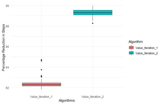
Figure 1.
Step reduction with Algorithms 1 and 2 against standard backward value iteration.
- Algorithm 1 operates without relying on any structural assumptions regarding the demand transition matrix. By leveraging the structural properties established in Theorem 1 (structuredness of capacity expansion decisions), Theorem 2 (structuredness of capacity reduction decisions), and Theorem 3 (monotonicity of optimal actions with respect to the capacity state), it achieves an average reduction of 82% in the required number of computational steps.
- Algorithm 2 extends these results by leveraging additional structural properties. Beyond the preceding theorems, it incorporates Theorem 4, which establishes the monotonicity of optimal actions with respect to the demand state under first-order stochastic dominance of the demand transition probabilities. Exploiting this structure yields substantial gains in computational efficiency, with average reductions in computational effort exceeding 87%.
Analogous to threshold maintenance policies and base-stock policies in maintenance and production, structured policies make MDP-based capacity planning intuitive for decision makers. They turn state-by-state optimization into clear rules that managers can check and follow. In the context of the monotonicity results (Theorems 1 and 2), the system admits two targets: a level to expand to and a level to shrink to. As a result, one only needs to solve exactly at the capacity bounds; for any interior capacity, the optimal move is simply the gap to the relevant target. This collapses the search space, speeds up computation substantially (with about an 82% average reduction when employing Algorithm 1), and yields straightforward, defensible guidance on when and how much to adjust capacity.
5. Numerical Examples
This section presents two examples to demonstrate the structural properties of the model presented in this paper.
Example 1.
Consider a problem where a system adjusts its capacity to fulfil demands. Any unit increase in the capacity costs the system USD 13, while any reduction in the capacity costs the system USD 4. The cost of maintaining the unit system capacity per period is USD 12. The cost of using one unit for the capacity to meet demand (operating cost) during a period is USD 24. The penalty incurred for each unit of demand exceeding the system capacity in a period is USD 65. The cost of salvaging the unit capacity at the end of planning horizon is −USD 3 (represents revenue). We need to find an optimal decision policy for capacity planning for a planning horizon of 10 periods. The maximum capacity level of the system is 10 units, and capacity decisions are made at the end of every period.
Problem parameters
The demand transition matrix is
The objective is to minimize the total cost over the planning horizon.
Optimal solution
The optimal solution to Example 1 is provided and demonstrated in Table 2, Table 3 and Table 4 and Figure 1 and Figure 2. The tables demonstrate that the optimal actions are monotonic for all levels of system capacity and do not change depending on the demand, as shown in Figure 2.
Table 2.
Example 1, optimal actions at t = 1, 2, 3.
Table 3.
Example 1, optimal actions at t = 4 ().
Table 4.
Example 1, optimal actions at t = 5 ().
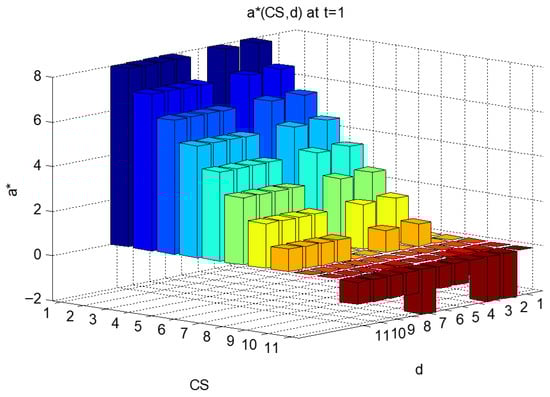
Figure 2.
Example 1, Graphical representation I of the optimal decision rule at t = 1 (Table 2).
The same pattern repeats for the optimal decision rules for periods 6, 7, and 8, which we will skip. Figure 2 and Figure 3 demonstrate the optimal decision rules when .
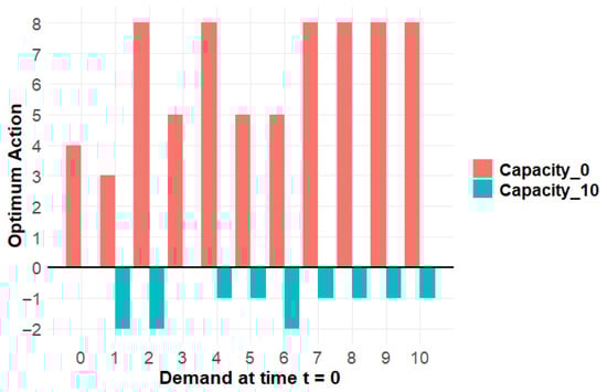
Figure 3.
Example 1, Graphical representation II of the optimal decision rule at t = 1. Capacity_0 is the action carried out at minimum capacity , and Capacity_10 is the action caried out at maximum capacity
Upon analysing the optimal decision at different time epochs, we find that the result is in accordance with our listed theorems:
- After determining , we see that, with every unit increase in , decreases by 1 unit until it reaches 0. This follows from Theorem 1.
- After determining , we see that, with every unit decrease in , increases by 1 unit until it reaches 0. This follows from Theorem 2.
- For a given , does not increase with . This follows from Theorem 3.
Theorems 1–3 allow a simpler representation of the policy in Figure 2, which is given in Figure 4. Essentially, knowing the optimum policy at maximum and minimum capacity levels for a demand defines the optimal policy for the remaining capacity levels.
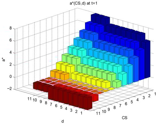
Figure 4.
Example 2, Graphical representation of optimal decision rule at t = 1.
Example 2.
In this example, we work on the same problem parameters as in Example 1, but, now, we replace the demand transition matrix with one that has first-order stochastic dominance, as given below.
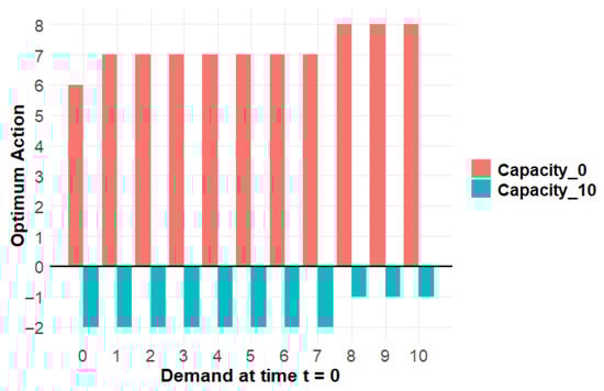
Figure 5.
Example 2, Graphical representation II of optimal decision rule at t = 1.
Upon analysing the optimal decision at different time epochs, we find that the result is in accordance with our listed theorems:
- Theorems 1–3 are upheld, as described in Example 1; and since this problem definition has a demand matrix satisfying first-order stochastic dominance, for a given , does not decrease with . This follows from Theorem 4. Figure 3 and Figure 5 demonstrate that the results become more structured when the conditions of Theorem 4 hold true.
6. Summary
This study presents the formulation of a finite-horizon Markov decision process (MDP) for addressing capacity planning challenges characterized by time-variant Markovian demand. The approach integrates both capacity expansion and contraction within a generic cost structure. This research identifies two fundamental and practical cost conditions that facilitate the development of a simplified policy structure. Furthermore, when demand transitions adhere to first-order stochastic dominance, an additional property of monotonicity is established. We also leverage the property of convexity to enhance the value iteration process, thereby reducing computational effort.
In finite-horizon, time-varying contexts, optimal policies may appear counterintuitive. This study has established sufficient cost conditions (including when assuming there is first-order stochastic dominance (FOSD)), where these policies simplify to straightforward, verifiable rules. (i) State-contingent targets indicate that if expanding to level g is optimal at a certain capacity, the same target is applicable from any lower capacity; conversely, if contracting to level e is optimal, the same target applies for any higher capacity. (ii) There is a monotonicity with respect to capacity such that with increased installed capacity, the prescribed expansions are not larger. (iii) There is monotonicity across demand states, where under FOSD, higher demand states do not necessitate smaller adjustments. This policy is computationally efficient, facilitating routine and defensible decisions regarding capacity.
Finally, our study was conducted under the following simplifying assumptions: (i) transition probability matrices are known, (ii) capacity adjustment lead times are zero, and (iii) the system features a single, homogeneous capacity type. These assumptions facilitated structural characterization of the optimal policies but limit the external validity and practical generalizability of the results. Future research could relax these restrictions by (a) statistically estimating or learning the transition dynamics from data (through model-free reinforcement learning); (b) incorporating strictly positive and stochastic lead times, including ramp-up and ramp-down dynamics together with potentially nonconvex capacity adjustment costs; and (c) extending the model to multi-resource systems (e.g., multiple nonidentical resources) with explicit coupling constraints across resources. Moreover, empirical calibration using industry data and data-driven policy optimization or evaluation would allow a more rigorous assessment of the managerial relevance and performance of the proposed decision rules.
Author Contributions
Methodology, J.A. and M.M.A.; validation, J.A. and M.M.A.; formal analysis, J.A. and M.M.A.; writing—original draft, J.A. and M.M.A.; writing—review and editing, J.A. and M.M.A.; supervision, M.M.A. All authors have read and agreed to the published version of the manuscript.
Funding
The authors would like to acknowledge the support provided by the Deanship of Research at King Fahd University of Petroleum & Minerals (KFUPM).
Data Availability Statement
The original contributions presented in this study are included in the article. Further inquiries can be directed to the corresponding author.
Conflicts of Interest
The authors declare no conflicts of interest.
Appendix A
This section lists the theorems, propositions, and lemmas of Section 4 along with their detailed proofs.
Proof of Theorem 1:
The proof of Theorem 1 is shown by contradiction. Conceptually, given an optimal action such that , we obtain a set of different relations (necessary optimality conditions) by acknowledging that for the different possible values of , except in the case of increasing the system’s capacity to level . Now, if in states , where , there exist better actions than increasing the system capacity to reach the same capacity level , we obtain a second set of relations. However, it will be shown that this set of relations will contradict the first set; hence, the optimal action is to reach capacity level . Next, we provide the detailed proof of this theorem:

Figure A1.
Theorem 1 capacity level illustration.
Graphically, Figure A1 represents a set of capacities , where
Given the optimal action and , referring to Figure A1, let us consider all possible alternative actions:
Let be any action such that
Let be any action such that
Let be any action such that
Let be any action such that
Based on this, since is the optimal action at , we are left with the following four relations (necessary optimality conditions on ):
- (1)
- .
- (2)
- .
- (3)
- .
- (4)
- .
Relations 1–4 imply that, in any time period, the value function when the optimal action is carried out will be always less than or equal to the value function at the time when any other action is carried out.
Taking one relation at a time:
- (1)
- .
By substituting in Equation (7), using Equation (3), and simplifying, we get
By applying the same approach to the remaining relations, we get
- (2)
- ,
- (3)
- ,
- (4)
- ,
Given a capacity CS2 such that , let us consider all possible actions available for the state (other than the action ):
Action Subset 1: This is an action such that
Action Subset 2: Let be any action such that
Action Subset 3: Let be any action such that
Action Subset 4: Let be any action such that
Let be the action such that
If in state an action in action Subset 1 yields a better value function than that corresponding to action , then
By writing the value function Equation (7) and using Equation (3), we get
We can see that Equation (A5) contradicts Equation (A1). This implies that action cannot be better than action
Similarly, for action subsets 2, 3, and 4, we get the following relations:
It is obvious that Equations (A6)–(A8) contradict Equations (A2)–(A4), respectively. Hence, actions , or cannot be better than action
Thus, is the optimal action at . This completes the proof of Theorem 1. □
Proof of Theorem 2:
Similar to Theorem 1, the proof of Theorem 2 is shown by contradiction. Conceptually, given an optimal action such that , we obtain one set of relations (necessary optimality conditions) by acknowledging that . Now, if in states , where , there exist better actions than decreasing the system capacity to reach the same capacity level , we obtain a second set of relations. However, it will be shown that this set of relations will contradict the first set. Hence, the optimal action is to reach capacity level. Next, we provide the detailed proof of this theorem.

Figure A2.
Theorem 2 capacity level illustration.
Graphically, Figure A2 represents a set of capacities , where
Given the optimal action and
Referring to Figure A2, let us consider all possible alternative actions:
Let be any action such that
Let be any action such that
Let be any action such that
Let be any action such that
Since is the optimal action at , we are left with the following relations (necessary optimality conditions on ):
- (1)
- .
- (2)
- .
- (3)
- .
- (4)
- .
Relations 1–4 imply that, in any time period, the value function for the optimal action will always be less than or equal to the value function for any other action.
We will employ one relation at a time:
- (1)
- .
By substituting in Equation (7), using Equation (3), and simplifying, we get
- (2)
- Doing the same with the remaining relations, we get , which yields
- (3)
- yields
- (4)
- yields
Given a capacity CS1 such that , let us consider all possible actions available for the state
Action Subset 1: Let be any action such that
Action Subset 2: Let be any action such that
Action Subset 3: Let be any action such that
Action Subset 4: Let be any action such that
Let be the action such that
If in state an action in action subset yields a better value function than that corresponding to action , then
By writing the value function Equation (7) and using Equation (3), we get
We can see that Equation (A13) contradicts Equation (A9). This implies that action cannot be better than action .
Similarly, we get the following relations for action subsets 2, 3, and 4:
Equations (A14)–(A16) are in contradiction to relations (A10)–(A12), respectively.
Hence, there cannot exist a better action at than . This completes the proof of Theorem 2. □
Proof of Lemma 2:
superadditive in ∀ means that for any in :
is nondecreasing in
It can be observed that as increases, can have at most three regions in the following order:
- (1)
- (2)
- (3)
Region 1:
Note that based on the cost parameter assumption , the relation is implicit. Hence, in region 1, is a constant with a negative value
Region 2:
Since , increases with an increase in . However, as , the value is negative.
Region 3:
From the above analysis, we get is nondecreasing in .
This completes the proof of Lemma 2. □
Proof of Proposition 1:
The proof of this proposition is established using mathematical induction. This starts from the last time epoch , where the capacity is to be salvaged. We work our way up, showing that the value function and its components are superadditive in ∀
From Equation (2),
Since for any and for any combination of and , is superadditive in ∀ . Note that in practice, there is virtually no other option in the last epoch but to salvage the capacity. We simply make this manipulation to lay out the proof.
Writing Equation (7)
Considering the elements of this equation, from Equation (3):
This is because is a constant independent of ∀ . We have as a superadditive in ∀ .
Hence, will be superadditive in , if is superadditive in
Moreover, if is superadditive in , then will be superadditive in
In conclusion, if is superadditive in , then will be superadditive in ∀
This will be shown to be true for our problem definition via induction:
Since , we have as a superadditive in , because for any two actions and in such that , we have
The term is independent of .
By employing Equation (7) for and substituting Equations (3) and (A17), we acquire
We can see that is superadditive in .
From Equation (A18), based on the assumption on the cost parameters , there are three possible optimal actions at depending on the measurement of with respect to and :
if ; we thus get
if , so we have
if , so we have
Next, we have the Bellman optimality equation for , which depends on , as follows:
As shown earlier, if is superadditive in , then will be superadditive in ∀ .
Let be two actions such that
We have for the three cases as follows:
The first parts in Equation (A19)
are constants. By studying the second part of Equation (A19), , based on Lemma 2, we find that it increases in
This means is increasing in . This gives the superadditive in
So far, the following results have been established:
- 1.
- are superadditive in , respectively.
- 2.
- are superadditive in , respectively.
This gives the first step of the induction proof of Proposition 1. Next, assuming that and are both superadditive in we need to prove that is superadditive in to prove that is superadditive in
That is, we need to check if is nondecreasing in for any
Let the optimal action in time epoch and state be
This implies that when in state , , based on Theorem 1.
And let optimal action in time epoch and state be
This implies that when in state , , based on Theorem 2. Moreover, Theorems 1 and 2 imply that .
Let ( and are special cases of this).
To study the nature of with an increase in for a given , we have two possibilities depending on the selection of and :
Possibility 1:
In this region,
This gives
In this region,
This gives
Equation (A25) implies that for a unit increase in , the last part (Equation (A24)) is nondecreasing in
When

Figure A3.
Proposition 1: Possibility 1— regions.
As shown in Figure A3 for Possibility 1, the resulting regions are considered:
Region I:
In this region, in both functions
This implies
Based on Theorem 1, the optimal action would be to go to capacity for both states and ; hence,
Simplifying
Lemma 2 shows that is nondecreasing in
Hence, in region I, is superadditive in
Region II:
in the function and in the function
This implies
Based on Theorems 1 and 2, the optimal action would be to go to capacity for states and to choose action for states
We study Equation (A20) in parts:
- 1.
- is fixed in this region.
- 2.
- Lemma 2 shows is nondecreasing in .
- 3.
- The last part is as follows:
Equation (A22) implies that for a unit increase in , the decrease in in Equation (A21) will not be more than
This shows that in the last part, is nondecreasing in
Hence, in region II, is superadditive in .
Region III:
in both the functions and
This implies
is a fixed value. Lemma 2 shows is nondecreasing in . is nondecreasing in , because is superadditive in
Hence, in region III, is superadditive in
Region IV:
in the function and in the function .
This implies
Equation (A23) is studied in parts:
- 1.
- is fixed in this region.
- 2.
- Lemma 2 shows is nondecreasing in .
- 3.
- The last part is as follows:
Hence, in region IV, is superadditive in .
Region V:
in both functions and
This implies
does not change with an increase in . Lemma 2 shows is nondecreasing in . Hence, in region V, is superadditive in
This completes the proof of Possibility 1 when . □
Now, we move onto Possibility 2 when . The proof process is the same as in Possibility 1, which we just addressed.
Possibility 2:
When

Figure A4.
Proposition 1, Possibility 2— regions.
As shown in Figure A4 for Possibility 2, the resulting regions are considered:
Region I:
in both functions .
This implies
This is the same as region I for Possibility 1.
Hence, in region I, is superadditive in .
Region 2:
in the function , and in the function . This implies
The region is the same as region II of Possibility 1.
Hence, in region II, is superadditive in .
Region III:
in the function and in the function . This implies
We study Equation (A26) in parts:
- 1.
- is a fixed value in this region upon an increase in .
- 2.
- Lemma 2 shows is nondecreasing in
- 3.
- increases with , considering the assumption that .
Hence, in region III, is superadditive in .
Region IV:
in the function , and in the function . This implies
The region is given the same consideration as region IV of Possibility 1.
Hence, in region IV, is superadditive in
Region V:
The same consideration is given for region V for Possibility 1. Hence, in region V, is superadditive in
This completes the proof of Possibility 2. □
We have thus shown that is superadditive in in the given model if and are superadditive in
We have thus proved by induction that is superadditive in ∀
Proof of Theorem 4:
From Equations (3) and (7),
; this gives
And ; this gives
Considering the assumption , is nondecreasing in if is nondecreasing in
From the Proof of Proposition 1, we have shown that is superadditive in
Thus, ∀ such that and ; it follows
Let . This yields
Equation (A27) implies that is nondecreasing in , thus completing the proof of Theorem 4. □
Proof of Lemma 3:
To state is subadditive in ∀ means ∀ in :
is nonincreasing in .
has three regions:
- (1)
- (2)
- (3)
Region 1:
Region 2:
Note that based on the cost parameter assumption , the relation is implicit. Hence, the above relation decreases with .
Region 3:
Hence, we have nonincreasing in . □
Proof of Proposition 2:
The proof of this proposition is quite similar to the proof of Proposition 1 and is also established using mathematical induction. This starts from the last time epoch T, where the capacity is to be salvaged. □
From Equation (2),
for any , and any combination of and . Hence, we find that is subadditive in ∀ .
We write Equation (7) as follows:
Considering the elements of this equation,
is subadditive in ∀ because
is a constant independent of (∀).
Hence, will be subadditive in , if is subadditive in .
Moreover, since shows first-order stochastic dominance will be subadditive in if is subadditive in .
In conclusion, will be subadditive in ∀ , if is subadditive in .
This will be shown by induction:
Starting with the last period , since , is subadditive in , as for :
is independent of .
From Equation (A18),
It is evident that is subadditive in .
From Equation (A19), it is shown for :
The first parts of Equation (A19) are constants. The second part of Equation (A19) is known to be nonincreasing in from Lemma 3. Similar arguments can be made for cases and . The proofs are straightforward and hence skipped here.
This means is nonincreasing in . This shows that is subadditive in
So far, the following results have been established:
- 1.
- is subadditive in , respectively.
- 2.
- is subadditive in , respectively.
This results in the first step of the induction proof of the proposition. Next, assuming that and are subadditive in we need to prove that is subadditive in to prove that is subadditive in
That is, we must check if is nonincreasing in for any
Let the optimal action in time epoch and state be
And let the optimal action in time epoch and state be
The understanding here is the same as explained for Proposition 1.
From Theorems 1 and 2, it is understood that
Let (and will be special cases of this).
The following steps in the proof are parallel to those explained in the proof of Proposition 1; again to study the nature of with an increase in for a given , we have two possibilities depending on the selection of and :
Possibility 1:
is nonincreasing in because shows first-order stochastic dominance and is subadditive in
When

Figure A5.
Proposition 2, Possibility 1— regions.
As shown in Figure A5 for Possibility 1, the resulting regions are considered:
Region I:
In this region, in both functions
This implies
Based on Theorem 1, the optimal action would be to go to capacity for both states and ; hence,
We will simplify:
Lemma 3 shows is nonincreasing in
Hence, in region I, is subadditive in .
Region II:
in the function , and in the function ; this implies
Based on Theorems 1 and 2, the optimal action would be to go to capacity for states and to choose action for states :
We study Equation (A28) in parts:
- 1.
- is fixed in this region.
- 2.
- Lemma 3 shows is nonincreasing in .
- 3.
- The last part is as follows:
- 4.
- is nonincreasing in because shows first-order stochastic dominance and is subadditive in .
Hence, in region II, is subadditive in .
Region III:
in both the functions and
This implies
is a fixed value. Lemma 3 shows is nonincreasing in . is shown to be nonincreasing in , because is subadditive in .
Hence, in region III, is subadditive in .
Region IV:
in the function , and in the function .
This implies
We study Equation (A29) in parts:
- 1.
- is fixed in this region.
- 2.
- Lemma 3 shows is nonincreasing in .
- 3.
- The last part is as follows:
Hence, in region IV, is subadditive in
Region V:
in both functions and
This implies
is constant with an increase in . Lemma 3 shows is nonincreasing in . Hence, in region V, is subadditive in
This completes the proof of Possibility 1 when . □
Now we move onto Possibility 2 when . The proof process is the same as in Possibility 1, which we just addressed. Again, the steps are parallel to the proof of Proposition 1.
Possibility 2
When .

Figure A6.
Proposition 2, Possibility 2 regions.
As shown in Figure A6 (above) for Possibility 1, the resulting regions are considered:
Region I:
in both functions .
This implies
This is the same as region I for Possibility 1.
Hence, in region I, is subadditive in .
Region II:
in the function and in the function
This implies
The region is given the same consideration as region II of Possibility 1.
Hence, in region II, is subadditive in .
Region III:
in the function , and in the function
This implies
We study Equation (A30) in parts:
- is a fixed value in this region.
- Lemma 3 shows is nonincreasing in
- is nonincreasing with because shows first-order stochastic dominance and is subadditive in
Hence, in region III, is subadditive in .
Region IV:
in the function , and in the function
This implies
The region is given the same consideration as region IV of Possibility 1.
Hence, in region IV, is subadditive in
Region V:
This is the same as region V of Possibility 1.
Hence, in region V, is subadditive in . This completes the proof of Possibility 2.
We have now shown that under first-order stochastic dominance of demand transition matrix and if is subadditive in and is subadditive in then is subadditive in , showing that is subadditive in
This completes the proof of Proposition 2. □
References
- AlDurgam, M.M.; Tuffaha, F.M.; Abdel-Aal, M.A.M.; Almoghathawi, Y.; Saleh, H.H.; Saleh, Z. A Scientometric Analysis of the Capacity Expansion and Planning Research. IEEE Trans. Eng. Manag. 2024, 71, 6382–6405. [Google Scholar] [CrossRef]
- Fu, C.; Suo, R.; Li, L.; Guo, M.; Liu, J.; Xu, C. A Capacity Expansion Model of Hydrogen Energy Storage for Urban-Scale Power Systems: A Case Study in Shanghai. Energies 2025, 18, 5183. [Google Scholar] [CrossRef]
- Hole, J.; Philpott, A.B.; Dowson, O. Capacity Planning of Renewable Energy Systems Using Stochastic Dual Dynamic Programming. Eur. J. Oper. Res. 2025, 322, 573–588. [Google Scholar] [CrossRef]
- AlDurgam, M.M. An Integrated Inventory and Workforce Planning Markov Decision Process Model with a Variable Production Rate. IFAC-PapersOnLine 2019, 52, 2792–2797. [Google Scholar] [CrossRef]
- Conejo, A.J.; Hall, N.G.; Long, D.Z.; Zhang, R. Robust Capacity Planning for Project Management. Inf. J. Comput. 2021, ijoc.2020.1033. [Google Scholar] [CrossRef]
- Kováts, P.; Skapinyecz, R. A Combined Capacity Planning and Simulation Approach for the Optimization of AGV Systems in Complex Production Logistics Environments. Logistics 2024, 8, 121. [Google Scholar] [CrossRef]
- Teerasoponpong, S.; Sopadang, A. A Simulation-Optimization Approach for Adaptive Manufacturing Capacity Planning in Small and Medium-Sized Enterprises. Expert Syst. Appl. 2021, 168, 114451. [Google Scholar] [CrossRef]
- Chien, C.-F.; Wu, C.-H.; Chiang, Y.-S. Coordinated Capacity Migration and Expansion Planning for Semiconductor Manufacturing under Demand Uncertainties. Int. J. Prod. Econ. 2012, 135, 860–869. [Google Scholar] [CrossRef]
- Aldurgam, M.M. Dynamic Maintenance, Production and Inspection Policies, for a Single-Stage, Multi-State Production System. IEEE Access 2020, 8, 105645–105658. [Google Scholar] [CrossRef]
- Puterman, M.L. Markov Decision Processes: Discrete Stochastic Dynamic Programming, Wiley Series in Probability and Statistics; 1st ed.; Wiley: Hoboken, NJ, USA, 1994; ISBN 978-0-471-61977-2. [Google Scholar]
- Wu, C.-H.; Chuang, Y.-T. An Efficient Algorithm for Stochastic Capacity Portfolio Planning Problems. J. Intell. Manuf. 2012, 23, 2161–2170. [Google Scholar] [CrossRef]
- Krishnamurthy, V. Interval Dominance Based Structural Results for Markov Decision Process. Automatica 2023, 153, 111024. [Google Scholar] [CrossRef]
- Lee, S.J.; Gong, X.; Garcia, G.-G. Modified Monotone Policy Iteration for Interpretable Policies in Markov Decision Processes and the Impact of State Ordering Rules. Ann. Oper. Res. 2025, 347, 783–841. [Google Scholar] [CrossRef]
- Martínez-Costa, C.; Mas-Machuca, M.; Benedito, E.; Corominas, A. A Review of Mathematical Programming Models for Strategic Capacity Planning in Manufacturing. Int. J. Prod. Econ. 2014, 153, 66–85. [Google Scholar] [CrossRef]
- Wu, C.-H.; Chuang, Y.-T. An Innovative Approach for Strategic Capacity Portfolio Planning under Uncertainties. Eur. J. Oper. Res. 2010, 207, 1002–1013. [Google Scholar] [CrossRef]
- Lin, J.T.; Chen, T.-L.; Chu, H.-C. A Stochastic Dynamic Programming Approach for Multi-Site Capacity Planning in TFT-LCD Manufacturing under Demand Uncertainty. Int. J. Prod. Econ. 2014, 148, 21–36. [Google Scholar] [CrossRef]
- Mishra, B.K.; Prasad, A.; Srinivasan, D.; ElHafsi, M. Pricing and Capacity Planning for Product-Line Expansion and Reduction. Int. J. Prod. Res. 2017, 55, 5502–5519. [Google Scholar] [CrossRef]
- Serrato, M.A.; Ryan, S.M.; Gaytán, J. A Markov Decision Model to Evaluate Outsourcing in Reverse Logistics. Int. J. Prod. Res. 2007, 45, 4289–4315. [Google Scholar] [CrossRef]
- Abduljaleel, J.; AlDurgam, M. Structured Optimal Policy for a Capacity Expansion Model Using Markov Decision Processes. In Proceedings of the 2024 IEEE International Conference on Technology Management, Operations and Decisions (ICTMOD), Sharjah, United Arab Emirates, 4–6 November 2024; IEEE: Sharjah, United Arab Emirates, 2024; pp. 1–7. [Google Scholar]
- Blancas-Rivera, R.; Cruz-Suárez, H.; Portillo-Ramírez, G.; López-Ríos, R.; Blancas-Rivera, R.; Cruz-Suárez, H.; Portillo-Ramírez, G.; López-Ríos, R. (s, S) Inventory Policies for Stochastic Controlled System of Lindley-Type with Lost-Sales. MATH 2023, 8, 19546–19565. [Google Scholar] [CrossRef]
- Van Jaarsveld, W.; Arts, J. Projected Inventory-Level Policies for Lost Sales Inventory Systems: Asymptotic Optimality in Two Regimes. Oper. Res. 2024, 72, 1790–1805. [Google Scholar] [CrossRef]
- Yuan, S.; Lyu, J.; Xie, J.; Zhou, Y. Asymptotic Optimality of Base-Stock Policies for Lost-Sales Inventory Systems with Stochastic Lead Times. Oper. Res. Lett. 2024, 57, 107196. [Google Scholar] [CrossRef]
- Beyer, D.; Sethi, S.P.; Taksar, M. Inventory Models with Markovian Demands and Cost Functions of Polynomial Growth. J. Optim. Theory Appl. 1998, 98, 281–323. [Google Scholar] [CrossRef]
Disclaimer/Publisher’s Note: The statements, opinions and data contained in all publications are solely those of the individual author(s) and contributor(s) and not of MDPI and/or the editor(s). MDPI and/or the editor(s) disclaim responsibility for any injury to people or property resulting from any ideas, methods, instructions or products referred to in the content. |
© 2025 by the authors. Licensee MDPI, Basel, Switzerland. This article is an open access article distributed under the terms and conditions of the Creative Commons Attribution (CC BY) license (https://creativecommons.org/licenses/by/4.0/).