Abstract
In this paper, we investigate the optimal control problem regarding a class of dynamic systems, aiming to address the challenge of simultaneously ensuring cost minimization and system asymptotic stability. The theoretical framework proposed in this paper integrates the value function concept from optimal control theory with Lyapunov stability theory. By setting the impulse cost at any finite time to be strictly positive, we exclude Zeno behavior, and a set of sufficient conditions is established that simultaneously guarantees system asymptotic stability and cost minimization based on Quasi-Variational Inequalities (QVIs). To address the challenge of solving the Hamilton–Jacobi–Bellman (HJB) equation in high-dimensional nonlinear systems, we employ an inverse optimal control framework to synthesize the strategy and its corresponding cost function. Finally, we validate the feasibility of our method by applying the theoretical results obtained to three numerical examples.
Keywords:
impulsive control; asymptotic stability; Hamilton–Jacobi–Bellman equation; Quasi-Variational Inequalities; Lyapunov function MSC:
49N25
1. Introduction
Impulsive systems play an important role in modeling modern engineering processes where continuous evolution coexists with instantaneous jumps. Such dynamics arise naturally in networked control, robotics, power systems, and biological processes [1,2,3,4,5,6,7]. The theory of impulsive differential equations, introduced in the 1960s [8], provides a formal foundation for analyzing these hybrid behaviors and has since been widely developed within the stability and control communities.
System stability is fundamental in control theory [9]. The framework of impulsive differential equations developed by Lakshmikantham et al. provides a basis for applying classical stability theory to impulsive systems [10]. Building on Lyapunov methods, many stability results have been established for impulsive and hybrid systems with delays, nonlinearities, and other complexities [4,11,12,13,14,15,16,17,18,19,20,21]. Representative examples include the stability of discrete-time impulsive delay neural networks [11], quaternion-valued neural networks with state-dependent impulses analyzed via the B-equivalence method [13], impulsive consensus in multi-agent systems using impulse edge event-triggered strategies [16], and lag synchronization under asymmetric saturation [20]. Recent progress also includes hybrid-system-based analyses of impulsive switching signals [22] and delay-compensatory impulsive control for delayed systems [23].
Another major research direction is optimal control of impulsive systems. The goal is to design impulsive moments and magnitudes that minimize a prescribed cost functional. One classical approach is based on the Minimum/Maximum Principle: early work addressed systems with a fixed number of impulses [24]. Based on [24], scholars developed first- and second-order necessary conditions for the Minimum Principle [25,26]. Subsequently, these theories were systematically generalized, leading to the formation of the Impulse Control Maximum Principle. This principle provides a complete set of necessary and sufficient conditions for deterministic impulsive control problems [27,28]. In recent years, it has been generalized to more complex stochastic systems, such as stochastic forward–backward systems involving conditional mean fields and regime switching [29] as well as general hybrid systems [30,31]. Another path of optimal impulsive control is based on the principle of Dynamic Programming. Its theoretical foundation traces back to the milestone work of Bensoussan and Lions [32], where the value function is closely linked to the HJB equation. Although these methods provide powerful tools for solving optimal impulsive control problems, they usually do not guarantee stability of the optimal strategy. In the field of continuous systems, L’Afflitto et al. established a theoretical framework for combining optimal control and system stabilization [33,34,35,36,37]. Recently, this strategy was also extended to the field of impulse disturbance, combining event-triggered mechanisms to study the system’s stability and equilibrium solutions [37]. However, determining how to control a continuously unstable system by applying impulses to simultaneously ensure optimal performance and asymptotic stability remains a challenge, and existing results in this specific area are still limited.
In view of this, this paper is dedicated to developing a theory for the optimal impulsive control and stabilization of dynamic systems. The objective is to design a control strategy that simultaneously achieves asymptotic stability and cost minimization. To this end, we integrate the value function from optimal control theory with Lyapunov stability theory. By combining stability conditions with the QVIs, a novel set of sufficient conditions is derived to simultaneously guarantee both asymptotic stability and performance optimality for the systems.
The main contributions of this paper are threefold: First, we prove that the optimal impulsive control strategy derived from the QVIs is free from Zeno behavior. Second, we construct a theoretical framework that unifies optimality and stabilization. By combining Lyapunov stability conditions with the QVIs, we propose a novel set of sufficient conditions. Any control policy that satisfies these conditions is guaranteed to simultaneously achieve both asymptotic stability and cost function minimization. Furthermore, to obtain the analytical solutions, we utilize the framework of inverse optimal control. Our third contribution lies in verifying the effectiveness of the proposed theory through numerical examples on a scalar linear system, a saddle-point system, and a nonlinear system. The simulation results clearly demonstrate that our designed optimal impulsive strategy not only successfully stabilizes the system to the origin but also results in a cost significantly lower than that of other impulsive control strategies.
The remainder of this paper is organized as follows. In Section 2, we present the problem formulation and some preliminaries. In Section 3, we establish the main theoretical results. Section 4 validates the effectiveness of our theoretical results through numerical simulations on different systems. Finally, ours conclusions are given in Section 5.
Notations: Let and be the real number set and positive real number set, and let and stand for the n-dimensional Euclidean space and the set of real matrices, respectively. denotes the integer set, and is the set of positive integers. I denotes the identity matrix with appropriate dimensions. The superscripts “−1” and “T” stand for the inverse and transpose of a matrix, respectively. represents Euclidean norm. A function belongs to class- if it is continuous, strictly increasing, and satisfies , .
2. Problem Statement and Preliminaries
We consider the following impulsive: system
where for every is an open set with , and , . Let be the set of admissible control, denote the impulsive control strategy, and denote the strategy set, where denotes the impulse moments, and denotes the corresponding impulse amplitude with . and denote the left and right limits, respectively, and, in this paper, it is assumed that the system is left-continuous, i.e., . Let . To account for the costs associated with system operation and the impulses, we define the following cost function:
where is the running cost, is the impulse cost, and is the discount factor. In this paper, we set . We make the following assumptions regarding the system (1) and the cost function (2).
Assumption 1.
The system and cost function are subject to the following requirements.
(i) is Lipschitz-continuous; i.e., there exists a constant such that
(ii) is Lipschitz-continuous in x; i.e., for , we have
(iii) The impulse cost function can be decomposed into the sum of two components, , where is the impulse-amplitude-dependent component, which is positive-definite with respect to the impulse amplitude , and is the time-dependent component, which is a strictly positive, bounded, and non-increasing function of time.
(iv) The running cost is positive-definite with respect to the state x. That is, holds for all , and for all .
(v) The functions L and G are locally Lipschitz-continuous with respect to their arguments on any compact subset of their domains.
Remark 1.
The conditions (i) and (ii) in Assumption 1 ensure the existence of a unique state trajectory for any measurable impulsive sequence . These regularity conditions are mild and are naturally satisfied by most mechanical, electrical, and robotic systems with smooth vector fields and bounded actuators. In Assumption 1.(iii), we set the impulse cost to be additively separable: , where increases with , reflecting the consumption of physical resources such as energy or fuel. The term represents an activation cost that is independent of the impulse amplitude and strictly positive, bounded, and non-increasing over time. This time-varying term can be used to model operational risks that are greater in the early stages of operation and gradually decrease as the system enters a more robust regime [38]. The decaying function models this time-varying operational risk. Assumption 1.(iv) ensures the running cost is accumulated as long as the system’s state deviates from the origin. This can always be achieved through standard quadratic or energy-based cost designs, such as with Assumption 1.(v) ensures the cost functions are bounded in any compact set. Because the cost functions L and G are typically continuous in practical designs, their local Lipschitz continuity in compact sets follows directly from the regularity imposed in Assumptions 1.(i)–(iii).
3. Main Results
We determine the cost-to-go function for strategy and for any initial system state as follows:
Then, the value function, denoted as , is
Remark 2.
Under Assumption 1, the value function is positive-definite and bounded by class- functions. These properties allow to be used directly as a Lyapunov function candidate in the stability analysis. The bounds also imply that grows unbounded as increases and ensure that the minimum cost for any non-zero initial state is strictly positive.
Assumption 2.
There exists a unique measurable function such that
Remark 3.
Under the continuity and coercivity of the cost components imposed in Assumption 1, the function admits a minimizer for compact sets, ensuring the existence of
To formally characterize the optimal control strategy under impulsive interventions, we introduce the intervention operators, which form the basis for the subsequent QVIs’ formulation. We define the intervention operator as follows:
Within this framework, the value function is assumed to satisfy the following QVIs:
Remark 4.
Inequality (5a) ensures that, in the absence of impulsive interventions, the value function evolves according to the HJB equation. Condition (5b) denotes that impulses are triggered at s only if the value function equals the sum of the impulse cost and the value function of the system state immediately after the impulses. The complementary condition (5c) ensures that, at any given moment, the strategy must be either to wait, ensuring that (5a) holds, or to apply an impulse to satisfy the intervention requirement.
Definition 1
([32]). Define the continuation set and intervention set as follows:
Theorem 1.
Proof of Theorem 1.
We prove our conclusion by contradiction. Assume that the system has a Zeno point, i.e., . Therefore, we have
according to Assumption 1.(iii). The impulse cost . And by using the definitions of the continuous set, the intervention set, and the operator (4), we are left with
By substituting (8) into (7) and using Assumption 1.(iii), we obtain
At the interval , the system dynamics are in continuation set and satisfy the HJB equation for the discounted problem:
The total time derivative of the value function along the system trajectory is . Substituting this into the HJB equation gives the evolution of between impulses:
As per Assumption 1.(v), is locally Lipschitz and and thus bounded in any compact subset. Since is continuous, it is also bounded in this compact set. Hence, there exist constants and such that and along the trajectory.
Therefore, the rate of change in the value function between impulses is also bounded; that is,
Next, consider the change in the value function from after just one impulse, , to the moment just before the next impulse, :
Therefore,
which means the change in between impulses is bounded by the length of the time interval. Now, we analyze the change in the value function over one full impulse period, from to :
Using the bounds from (9) and (10), we get
Taking the limit of both sides as , we arrive at
Since and are continuous, the left side becomes . And the first term on the right side approaches zero:
Thus, we find that . This is a contradiction to the assumption that . Thus, the proof is complete. □
According to Theorem 1, the impulsive control derived from QVIs does not exhibit Zeno behavior. Consequently, we provide a set of sufficient conditions that simultaneously ensure cost minimization and the asymptotic stability of the system.
Theorem 2.
Let Assumptions 1-2 hold. Suppose that there exists a function , wherein the positive constants α, , ε, and , are class- functions. is a strategy where
and the function also satisfies the following QVIs associated with the cost function (2). For all , the HJB inequality holds:
In the continuation set , the HJB equation holds:
and in the intervention region , an impulsive intervention is applied, and we have
Thus, the origin of system (1) under the strategy is globally asymptotically stable(GAS). Furthermore, the strategy minimizes cost function (2); that is,
where can be obtained as
Proof of Theorem 2.
In the interval between two impulses, the total derivative of is given by
Via Gronwall’s inequality, at interval , we have
In particular, at the instant just before the next impulse, we obtain
After using the impulse-triggering condition and the definition of (4), we arrive at
Considering the state jump relation , the preceding equation can be rewritten as
Next, we evaluate the evolution of to . We substitute (18) in (17) to obtain
By applying conditions (11f) and (11g), we arrive at
This result indicates that the sequence is strictly monotonically decreasing. Since is bounded below by zero, the sequence must converge, which guarantees that is bounded for all . Furthermore, in combination with (11c), it follows that is bounded for all time. Therefore, the zero solution of the system is Lyapunov-stable. Next, we prove that as . For ,
For ,
Specifically,
Furthermore, according to (11e) and (11g),
Thus, according to Theorem 1, the sequence of impulse moments is non-Zeno, and is positive-definite.
By virtue of (11c), the above result directly implies that
After combining Lyapunov stability with attractivity, we conclude that the origin of system (1) is GAS under the given impulsive control strategy.
Next, we obtain the following relation by solving for the integral of the full derivatives of between impulse intervals () at that interval time and summing over all :
The value function satisfies all
Therefore, we have
For the given impulse parameter level , according to the definition of the intervention operator given in (4), we obtain
Moreover, according to (5b), we have
Therefore, we have
By incorporating (24) and (27), we sum up i from 1 to infinity, so we obtain
Then,
Thus, we obtain
When we use the impulsive strategy , we have the following equality:
Through an argument similar to that used before, we obtain
Thus, the proof is complete. □
Remark 5.
Existing research has provided a significant foundation for optimal impulsive control. On the one hand, a great deal of research has been devoted to solving optimal impulsive control problems for dynamic systems [39,40,41,42]. Employing diverse methodologies, these studies have successfully optimized cost functions for various impulsive systems. However, within these frameworks, system stability has not been treated as a control objective co-designed with optimality. On the other hand, some works have begun to address control strategies that incorporate both stability and optimality [43,44,45,46], often relying on periodic or time-triggered mechanisms or on state-dependent triggering rules. In such frameworks, non-Zeno behavior is usually imposed as an assumption rather than derived as a consequence of control design. To address the aforementioned research gap, in this paper, we develop a unified framework that integrates stability, optimality, and non-Zeno properties. The sufficient conditions presented earlier that ensure asymptotic stability and cost minimization prove the absence of Zeno behavior under the optimal strategy.
In Theorem 2, we provide a set of sufficient conditions for verifying whether a given impulsive control strategy can simultaneously achieve asymptotic stability and cost function minimization. However, in many real-world engineering applications, control objects often manifest as high-dimensional nonlinear systems. In this context, directly solving the HJB equation is often extremely difficult or even impractical. To solve this problem and provide a more constructive and operational approach to strategy design, we will now adopt the design concept of inverse optimal control. Unlike solving for a given cost function in a forward manner, we first preset a candidate value function with a known structure based on the desired system performance (stability, convergence form, etc.), and then construct the cost function in a backward manner so that the constructed operating cost L can automatically satisfy the HJB equation.
Next, we will elaborate on this constructive design framework in Theorem 3 and provide analytical expressions for an optimal impulsive control strategy for system (1). To this end, we first specify the cost function in the following form:
where is a diagonal and positive-definite matrix. To construct an inverse optimal strategy for (1) and (28), let
where is a continuously differentiable, diagonal, and uniformly positive-definite matrix-valued function, and .
Theorem 3.
Consider the controlled nonlinear impulsive system (1) with cost function (28). Suppose there exists a continuously differentiable, symmetric, and uniformly positive-definite matrix-valued function ; a positive constant α; and an impulsive control strategy such that
are satisfied, and the resulting running cost function defined by
is positive-definite with respect to x. Then, the origin of system (1) under the impulsive control strategy is GAS. Furthermore, there exists a neighborhood of such that
where can be obtained in the following way:
Proof of Theorem 3.
Considering the Lyapunov function candidate defined by (29), the defined by (4), and the cost function (28), we have
Substitute (32) into (33):
Considering the QVI , we can obtain
By virtue of and ,
That is,
Thus,
When , impulses are triggered. By virtue of (30b), we arrive at
So, we can conclude that the origin of the system is asymptotically stable under strategy . According to condition (31), within the continuation region , we have
which implies (13). The feedback impulsive control level (32) follows from (15) by setting
Through strategy , the equality is satisfied at the impulse moments , which implies (14). The result now follows as a direct consequence of Theorem 2. □
4. Numerical Examples
In this section, we provide three numerical examples to validate the theoretical results presented previously. Specifically, we will demonstrate the asymptotic stability of the proposed optimal impulsive control strategy and verify its optimality by comparing its cost against several stabilizing but not optimal control strategies. Example 1 is a scalar linear system, Example 2 is a two-dimensional saddle-point system, and Example 3 is a two-dimensional nonlinear system.
4.1. Linear System
We consider the following scalar linear impulsive system:
where is impulse gain. We construct , where and the parameters are set to . Since the system should satisfy the HJB equation within the continuation set
we employ the framework of inverse optimal control to construct the running cost function :
Therefore, the cost function is given by
We set . Based on the preceding theory and the chosen parameters, the control gain for the optimal impulsive strategy is .
For comparison, we designed five suboptimal strategies. Among these strategies, the impulse moments of two of them remain consistent with the optimal strategy, but by changing the impulse amplitude to and , the other three replace the optimal impulse moments with different period-triggered ones ( s, s, and s) while keeping the optimal impulse amplitude unchanged. Their corresponding cost functions are denoted as , , , , and , respectively.
Figure 1 illustrates both the time evolution of the system trajectory under different impulsive control strategies and the trigger threshold. As depicted in the graph, the optimal control strategy successfully steers the system state towards the origin over time. This visually confirms that the system achieves asymptotic stability under the strategy, which is a prerequisite for the subsequent performance evaluation based on the cost function.
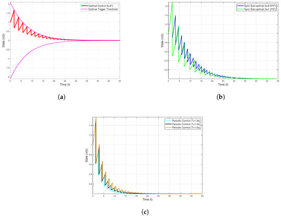
Figure 1.
Simulation of different control trajectories for system (34): (a) the trajectories of system (34) under the optimal impulsive control strategy and the threshold condition; (b) the trajectories of system (34) under the suboptimal impulsive control strategy; (c) and the trajectories of system (34) under the periodic impulsive control strategy.
The data presented in Figure 2 clearly illustrates the superiority of the proposed optimal impulsive control strategy. The simulated cost of the optimal strategy, , is equal to the theoretical optimal cost, . In contrast, the costs associated with the comparative strategies , , , , and are all significantly higher than the optimal cost. This confirms that for any given stabilization strategy, the cost is greater than the cost of the optimal strategy, verifying the optimality of the derived impulsive strategy, as established by the relationship . These numerical results provide strong validation of the theoretical framework developed in this paper.
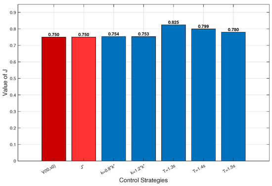
Figure 2.
Comparison of the cost functions of system (34).
4.2. Two-Dimensional Saddle-Point System
We consider the following two-dimensional saddle-point system:
where is the system state vector, and . Since the system matrix has eigenvalues , the uncontrolled continuous dynamics are unstable, indicating a canonical saddle-point system. Following the inverse optimal approach, we set , , where . From the QVI conditions, the optimal impulsive gain is derived as follows: Impulse events are triggered whenever the state norm reaches the following threshold: , .
The following parameters were chosen: . Two suboptimal strategies are designed with gains of and , and there are three periodic strategies with periods s, s, and s, respectively.
The simulation results in Figure 3 demonstrate that under the proposed optimal impulsive control strategy, both state components and converge asymptotically to zero, while the state norm remains strictly below the adaptive triggering boundary. All the comparative strategies yield higher total cost values. The results are summarized as follows:
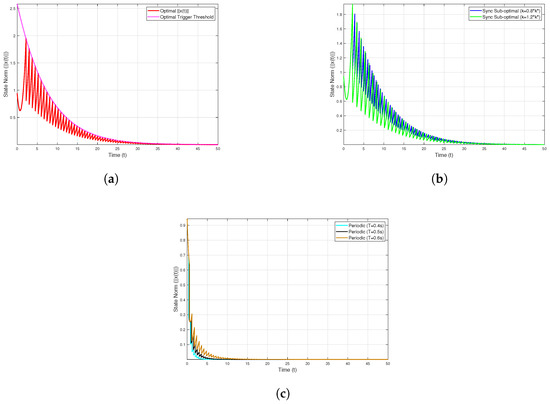
Figure 3.
Simulation of different control trajectories for system (35): (a) the trajectories() of system (35) under the optimal impulsive control strategy and the threshold condition; (b) the trajectories of system (35) under the suboptimal impulsive control strategy; (c) and the trajectories of system (35) under the periodic impulsive control strategy.
The results in Figure 4 confirm that the optimal impulsive control strategy achieves both asymptotic stability and a minimal cost, a finding fully consistent with the theoretical results established in Theorem 2.
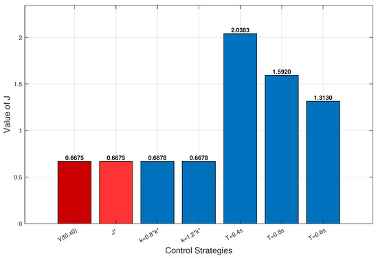
Figure 4.
Comparison of cost functions of system (35).
4.3. Nonlinear System
We consider the following two-dimensional nonlinear system:
where is the state vector, and is impulse gain. , , and the initial state is .
Following the inverse optimal approach, we set , where , and . This configuration yields the following running cost and corresponding cost function :
The cost function parameters are set as follows: discount factor , control cost weight , initial fixed impulse cost , , .
Based on these parameters, the optimal control gain was found to be . Similarly, the suboptimal impulse gains are set to and , respectively, and three periodic strategies’ impulse periods are set as follows: s, s, and s.
The results in Figure 5 show that all the control strategies successfully drive the system state towards the origin, demonstrating that the system is asymptotically stable under each strategy.
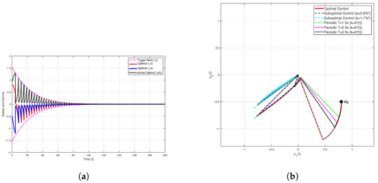
Figure 6 shows that which is equal to the theoretical optimum, . Crucially, the optimal strategy outperforms all the comparative strategies, yielding a total cost lower than that of strategies , , , , and These results validate the theoretical framework for the given nonlinear system.
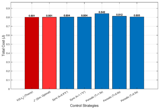
Figure 6.
Comparison of cost functions of system (36).
5. Conclusions
This paper has investigated the optimal impulsive control and stabilization problem pertaining to a class of dynamic systems, aiming to address the challenge of simultaneously ensuring cost function minimization and system asymptotic stability in traditional optimal control. Firstly, we have proven that the optimal strategy exhibits no Zeno behavior, thereby ensuring the physical feasibility of the strategy. Then, by integrating the value function concept from optimal control theory with Lyapunov stability theory, we have established a set of sufficient conditions that simultaneously guarantee system asymptotic stability and cost minimization. To address the challenge of solving the HJB equation, we further developed a method based on the framework of inverse optimal control. To validate the effectiveness of the proposed method, we applied the derived theoretical results to linear, saddle-point, and nonlinear systems and confirmed the feasibility of our method through numerical examples. There are several directions in which the work in this paper can be further expanded: (1) The proposed framework for deterministic systems can be extended to stochastic systems. (2) Future work can focus on developing efficient data-driven algorithms, such as Adaptive Dynamic Programming. (3) Another highly valuable research direction is to extend the current theoretical framework such that it includes systems with physical constraints such as actuator saturation and time delay. (4) Furthermore, extending the current theoretical framework to finite-time or fixed-time stability [47,48] would be a highly valuable research direction.
Author Contributions
W.W. and C.L.; methodology, W.W.; formal analysis, W.W.; investigation, W.W.; validation, M.H.; writing—original draft preparation, W.W.; writing—review and editing, C.L. and M.H.; supervision, C.L.; project administration, C.L.; funding acquisition, C.L. All authors have read and agreed to the published version of the manuscript.
Funding
This research is supported by the National Natural Science Foundation of China under Grant 62373310.
Data Availability Statement
The original contributions presented in this study are included in the article. Further inquiries can be directed to the corresponding author.
Conflicts of Interest
The authors declare no conflicts of interest.
References
- Zhang, L.; Lu, J.; Jiang, B.; Huang, C. Distributed synchronization of delayed dynamic networks under asynchronous delay-dependent impulsive control. Chaos Solitons Fractals 2023, 168, 113121. [Google Scholar] [CrossRef]
- Du, S.L.; Qiao, J.; Ho, D.W.; Zhu, L. Fixed-time cooperative relay tracking in multiagent surveillance networks. IEEE Trans. Syst. Man Cybern. Syst. 2018, 51, 487–496. [Google Scholar] [CrossRef]
- He, W.; Qian, F.; Han, Q.; Chen, G. Almost sure stability of nonlinear systems under random and impulsive sequential attacks. IEEE Trans. Autom. Control 2020, 65, 3879–3886. [Google Scholar] [CrossRef]
- Li, H.; Li, C.; Ouyang, D.; Nguang, S.K. Impulsive synchronization of unbounded delayed inertial neural networks with actuator saturation and sampled-data control and its application to image encryption. IEEE Trans. Neural Netw. Learn. Syst. 2020, 32, 1460–1473. [Google Scholar] [CrossRef] [PubMed]
- Chen, Y.; Zhao, Z. Mathematical model for continuous delayed single-species population with impulsive state feedback control. J. Appl. Math. Comput. 2019, 61, 451–460. [Google Scholar] [CrossRef]
- Qiu, R.; Li, R. Finite-time stability of spring-mass system with unilateral impact constraints and frictions. Mod. Phys. Lett. B 2020, 34, 2050341. [Google Scholar] [CrossRef]
- Cui, Q.; Li, L.; Lu, J.; Alofi, A. Finite-time synchronization of complex dynamical networks under delayed impulsive effects. Appl. Math. Comput. 2022, 430, 127290. [Google Scholar] [CrossRef]
- Milman, V.D.; Myshkis, A.D. On the stability of motion in the presence of impulses. Sib. Mat. Zhurnal 1960, 1, 233–237. [Google Scholar]
- Khalil, H.K.; Grizzle, J.W. Nonlinear Systems; Prentice Hall: Upper Saddle River, NJ, USA, 2002; Volume 3. [Google Scholar]
- Lakshmikantham, V.; Bainov, D.D.; Simeonov, P. Theory of Impulsive Differential Equations; World Scientific: London, UK, 1989; Volume 6. [Google Scholar]
- Li, C.; Wu, S.; Feng, G.G.; Liao, X. Stabilizing effects of impulses in discrete-time delayed neural networks. IEEE Trans. Neural Netw. 2011, 22, 323–329. [Google Scholar] [CrossRef]
- Guo, M.; Wang, P. Finite-time stability of non-instantaneous impulsive systems with double state-dependent delays. Appl. Math. Comput. 2024, 477, 128824. [Google Scholar] [CrossRef]
- Yang, X.; Li, C.; Song, Q.; Li, H.; Huang, J. Effects of state-dependent impulses on robust exponential stability of quaternion-valued neural networks under parametric uncertainty. IEEE Trans. Neural Netw. Learn. Syst. 2018, 30, 2197–2211. [Google Scholar] [CrossRef]
- Li, X.; Xing, Y.; Song, S. Nonlinear impulsive control for stability of dynamical systems. Automatica 2025, 178, 112371. [Google Scholar] [CrossRef]
- Liu, X.; Zeng, Y. Analytic and numerical stability of delay differential equations with variable impulses. Appl. Math. Comput. 2019, 358, 293–304. [Google Scholar] [CrossRef]
- Li, C.; Wang, W. Optimal Impulse Control and Impulse Game for Continuous-Time Deterministic Systems: A Review. Artif. Intell. Sci. Eng. 2025, 1, 208–219. [Google Scholar] [CrossRef]
- Zhao, Y.; Li, X.; Cao, J. Global exponential stability for impulsive systems with infinite distributed delay based on flexible impulse frequency. Appl. Math. Comput. 2020, 386, 125467. [Google Scholar] [CrossRef]
- Li, P.; Li, X.; Lu, J. Input-to-state stability of impulsive delay systems with multiple impulses. IEEE Trans. Autom. Control 2020, 66, 362–368. [Google Scholar] [CrossRef]
- Li, X.; Li, P. Stability of time-delay systems with impulsive control involving stabilizing delays. Automatica 2021, 124, 109336. [Google Scholar] [CrossRef]
- Wu, H.; Li, C.; He, Z.; Wang, Y.; He, Y. Lag synchronization of nonlinear dynamical systems via asymmetric saturated impulsive control. Chaos Solitons Fractals 2021, 152, 111290. [Google Scholar] [CrossRef]
- Gao, L.; Wang, D.; Wang, G. Further results on exponential stability for impulsive switched nonlinear time-delay systems with delayed impulse effects. Appl. Math. Comput. 2015, 268, 186–200. [Google Scholar] [CrossRef]
- Liu, S.; Tanwani, A. Impulsive switching signals with functional inequalities: Stability analysis using hybrid systems framework. Automatica 2025, 171, 111928. [Google Scholar] [CrossRef]
- Chen, L.; Cai, C.; Ling, S.; Lun, Y. Stability of delayed systems: Delay-compensatory impulsive control. ISA Trans. 2025, 167, 529–538. [Google Scholar] [CrossRef]
- Miller, B.; Rubinovich, E.J. Optimal impulse control problem with constrained number of impulses. Math. Comput. Simul. 1992, 34, 23–49. [Google Scholar] [CrossRef]
- Ahmed, N. Necessary conditions of optimality for impulsive systems on Banach spaces. Nonlinear Anal. Theory Methods Appl. 2002, 51, 409–424. [Google Scholar] [CrossRef]
- Arutyunov, A.; Jaćimović, V.; Pereira, F. Second order necessary conditions for optimal impulsive control problems. J. Dyn. Control Syst. 2003, 9, 131–153. [Google Scholar] [CrossRef]
- Chahim, M.; Hartl, R.F.; Kort, P.M. A tutorial on the deterministic impulse control maximum principle: Necessary and sufficient optimality conditions. Eur. J. Oper. Res. 2012, 219, 18–26. [Google Scholar] [CrossRef]
- Chahim, M. Impulse Control Maximum Principle: Theory and Applications; CentER, Center for Economic Research: Tilburg, The Netherlands, 2013. [Google Scholar]
- Wu, Z.; Zhang, Y. Maximum principle for conditional mean-field FBSDEs systems with regime-switching involving impulse controls. J. Math. Anal. Appl. 2024, 530, 127720. [Google Scholar] [CrossRef]
- Pakniyat, A.; Caines, P.E. On the hybrid minimum principle: The Hamiltonian and adjoint boundary conditions. IEEE Trans. Autom. Control 2020, 66, 1246–1253. [Google Scholar] [CrossRef]
- Clark, W.; Oprea, M. Symplectic Geometry in Hybrid and Impulsive Optimal Control. arXiv 2025, arXiv:2504.15117. [Google Scholar] [CrossRef]
- Bensoussan, A.; Lions, J.L. Optimal impulse and continuous control: Method of nonlinear quasi-variational inequalities. Tr. Mat. Instituta Im. V.A. Steklova 1975, 134, 5–22. [Google Scholar]
- Haddad, W.M.; L’Afflitto, A. Finite-time stabilization and optimal feedback control. IEEE Trans. Autom. Control 2015, 61, 1069–1074. [Google Scholar] [CrossRef]
- L’Afflitto, A.; Haddad, W.M.; Bakolas, E. Partial-state stabilization and optimal feedback control. Int. J. Robust Nonlinear Control 2016, 26, 1026–1050. [Google Scholar] [CrossRef]
- L’Afflitto, A. Differential games, continuous Lyapunov functions, and stabilisation of non-linear dynamical systems. IET Control Theory Appl. 2017, 11, 2486–2496. [Google Scholar] [CrossRef]
- L’Afflitto, A. Differential games, finite-time partial-state stabilisation of nonlinear dynamical systems, and optimal robust control. Int. J. Control 2017, 90, 1861–1878. [Google Scholar] [CrossRef]
- L’Afflitto, A. Differential games, partial-state stabilization, and model reference adaptive control. J. Frankl. Inst. 2017, 354, 456–478. [Google Scholar] [CrossRef]
- Naim, W. Data Importance in Power System Asset Management. Ph.D. Thesis, KTH Royal Institute of Technology, Stockholm, Sweden, 2024. [Google Scholar]
- Qi, Q.; Qiu, Z.; Ji, Z. Optimal continuous/impulsive LQ control with quadratic constraints. IEEE Access 2019, 7, 52955–52963. [Google Scholar] [CrossRef]
- Claeys, M.; Arzelier, D.; Henrion, D.; Lasserre, J.B. Measures and LMIs for impulsive nonlinear optimal control. IEEE Trans. Autom. Control 2013, 59, 1374–1379. [Google Scholar] [CrossRef]
- Avrachenkov, K.; Habachi, O.; Piunovskiy, A.; Zhang, Y. Infinite horizon optimal impulsive control with applications to Internet congestion control. Int. J. Control 2015, 88, 703–716. [Google Scholar] [CrossRef]
- Liu, X.; Li, S. Optimal control for a class of impulsive switched systems. J. Control Decis. 2023, 10, 529–537. [Google Scholar] [CrossRef]
- Haddad, W.M.; Nersesov, S.G.; Chellaboina, V. Energy-based control for hybrid port-controlled Hamiltonian systems. Automatica 2003, 39, 1425–1435. [Google Scholar] [CrossRef]
- Ramirez, N.F.; Ríos-Rivera, D.; Hernandez-Vargas, E.A.; Alanis, A.Y. Inverse optimal impulsive neural control for complex networks applied to epidemic diseases. Systems 2022, 10, 204. [Google Scholar] [CrossRef]
- Haddad, W.M.; Chellaboina, V.; Kablar, N.A. Non-linear impulsive dynamical systems. Part II: Stability of feedback interconnections and optimality. Int. J. Control 2001, 74, 1659–1677. [Google Scholar] [CrossRef]
- Hernandez-Mejia, G.; Alanis, A.Y.; Hernandez-Gonzalez, M.; Findeisen, R.; Hernandez-Vargas, E.A. Passivity-based inverse optimal impulsive control for influenza treatment in the host. IEEE Trans. Control Syst. Technol. 2019, 28, 94–105. [Google Scholar] [CrossRef]
- Cao, W.; Liu, L.; Ye, Z.; Zhang, D.; Feng, G. Resilient Global Practical Fixed-Time Cooperative Output Regulation of Uncertain Nonlinear Multi-Agent Systems Subject to Denial-of-Service Attacks. IEEE Trans. Autom. Control 2025. [Google Scholar] [CrossRef]
- Zhang, D.; Chen, H.; Lu, Q.; Deng, C.; Feng, G. Finite-time cooperative output regulation of heterogeneous nonlinear multi-agent systems under switching DoS attacks. Automatica 2025, 173, 112062. [Google Scholar] [CrossRef]
Disclaimer/Publisher’s Note: The statements, opinions and data contained in all publications are solely those of the individual author(s) and contributor(s) and not of MDPI and/or the editor(s). MDPI and/or the editor(s) disclaim responsibility for any injury to people or property resulting from any ideas, methods, instructions or products referred to in the content. |
© 2025 by the authors. Licensee MDPI, Basel, Switzerland. This article is an open access article distributed under the terms and conditions of the Creative Commons Attribution (CC BY) license (https://creativecommons.org/licenses/by/4.0/).