An Explicit Shifted Legendre Petrov–Galerkin Technique for the Time Fractional Cable Problem

Abstract

This paper focuses on analyzing and implementing a numerical technique using the Petrov–Galerkin technique (PGT) to solve the time fractional cable problem (TFCP). The trial functions are a modified set of shifted Legendre polynomials ($\mathsf{LPs}$). An appropriate numerical approach can be used to solve the linear algebraic equations resulting from the application of the PGT. With error bounds, we discuss the truncation estimation and stability in the $L_2$ norm. We apply some inequalities on the modified set of shifted $\mathsf{LPs}$ to this research. Numerical experiments include benchmark issues for which exact solutions are presented to show how efficient and accurate the method is. Comparisons with different techniques in the literature are used to support our examples.

1. Introduction

Fractional differential equations (DEs) appear in a variety of scientific and engineering disciplines. These equations are useful for modeling the electrical properties of real materials and for describing blood flow (see, for example, [1,2]). This paper focuses on solving a type of fractional DEs, namely, the TFCP.

The TFCE [3] is defined as follows:

$${\mathcal{X}}_t(\zeta ,t)=D_t^{1-{\beta }_1}\mu {\mathcal{X}}_{\zeta \zeta }(\zeta ,t)-\widehat{\nu }{D}_t^{1-{\beta }_2}\mathcal{X}(\zeta ,t)+f(\zeta ,t),0<{\beta }_1,{\beta }_2<1,$$

(1)

subject to the following conditions:

$$\mathcal{X}(\zeta ,0)={\mathcal{X}}_0\left(\zeta \right),\zeta \in (0,1),$$

(2)

$$\mathcal{X}(0,t)={\mathcal{X}}_1\left(t\right),\mathcal{X}(1,t)={\mathcal{X}}_2\left(t\right),t\in (0,1),$$

(3)

where non-negative $\mu$, $\widehat{\nu }$ are constants; ${\mathcal{X}}_0\left(\zeta \right),{\mathcal{X}}_1\left(t\right),{\mathcal{X}}_2\left(t\right)$ are given continuous functions; and $f(\zeta ,t)$ is the source term. Also, the symbol $D_t^{\beta }$ represents the operator of Caputo fractional derivative (FDs) of order $\beta$. Some researchers have investigated and offered several ways to solve TFCE. In Ref. [4], the authors suggested an efficient hybrid numerical technique to solve two-dimensional TFCEs. In Ref. [5], the author used two numerical methods to solve linear and nonlinear TFCEs. Furthermore, an improved method for the variable-order TFCE was developed in [6].

One of the most well-known numerical techniques [7,8,9] to solve different types of DEs is the use of spectral approaches. These approaches represent the solution as a finite set of basis functions and then transform the DEs to a system of computationally tractable algebraic equations. Collocation, tau, and Galerkin methods are the three primary approaches to these techniques. Many authors have followed these approaches to treat some types of DEs. For instance, developed shifted Chebyshev–Galerkin operational matrix approaches were presented by the authors of [10] for approximating partial boundary value problems of even order. The authors in [11] suggested a collocation technique for beam-type micro- and nanoscale BVP solutions. The tau technique was proposed by the authors in [12] for a bioheat transfer model in fractional framework. For more studies, see [13,14,15,16,17,18].

$\mathsf{LPs}$ have important applications in numerical analysis and approximation theory. Numerous papers related to numerical analysis made considerable use of these polynomials; for example, [19,20,21]. Also, many authors used these polynomials in many numerical techniques, for example, the authors in [22] used $\mathsf{LPs}$ to treat the two-point interface problems. Additionally, Heydari et al. [23] used $\mathsf{LPs}$ of the sixth kind for approximating the nonlinear fractal–fractional optimal control issues. In a porous channel, a numerical approach for handling the heat and mass transfer of a non-Newtonian fluid was also developed by Khan et al. [24] utilizing $\mathsf{LPs}$. Some other contributions regarding $\mathsf{LPs}$ can be found in [25,26].

Besides standard polynomial bases, many non-polynomial approximation methods have been presented for solving different types of DEs. For example, the authors in [27] used the non-polynomial spline method to solve linear fractional DEs. In [28], the authors presented a computation and discussion on non-polynomial splines of fractional order to solve the DEs with a Caputo FD. In [29], the authors proposed highly accurate solutions to the time-fractional KdV–Burgers equation employing rational non-polynomial splines. The authors in [30] introduced a numerical approach that combines conformable derivative, finite difference, and non-polynomial spline methods to address the nonlinear inhomogeneous time-fractional Burgers–Huxley equation.

The current article’s primary goals can be summed up in three points as follows:

• Introducing a novel method to solve the TFCP based on using the PGT along with the modified sets of shifted $\mathsf{LPs}$ as basis functions.
• Employing an appropriate strategy for solving a system resulting from the application of the PGT.
• Establishing closed relations for some integrals to construct the PGT.
• Analyzing the error analysis of the truncation error in $L_{w(\zeta ,t)}^2$ space.
• Presenting three illustrative examples to ensure that the PGT is accurate and applicable.
• Performing some comparisons with Ref. [31] to show the accuracy of the PGT.

The motivations for this article are listed in the following points:

• The TFCP is one of the most significant problems encountered in applied sciences. This encourages us to analyze it with a new technique.
• Several numerical methods were utilized to solve the TFCP using various orthogonal and non-orthogonal polynomials as basis functions. The basis functions utilized in this article are a set of orthogonal functions. This article encourages us to apply these functions to various problems in the applied sciences.
• To the best of our knowledge, the specific basis functions along with the PGT used in this paper were not previously used in numerical analysis, which provides a compelling reason to introduce and utilize them.

We note here that the novelty of this research includes the following points:

• Using modified sets of shifted $\mathsf{LPs}$ as basis functions allows us to take a few terms of the retained modes and obtain approximations with high precision compared to the basis of shifted $\mathsf{LPs}$.
• The employment of the presented basis functions along with the PGT for solving the TFCP is new.
• Some new operational relations are presented and employed.

The remaining sections of this work are arranged in the following manner. In Section 2, all required definitions and relations are reported. In Section 3, the PGT for treating the TFCP is discussed. The truncation error estimation and stability in $L_{w(\zeta ,t)}^2$ space are presented in Section 4. Some illustrative examples are given in Section 5 to show the accuracy of the proposed technique. Section 6 shows the result analysis of our proposed technique. Finally, Section 7 reports the conclusion.

2. Some Preliminaries and Essential Formulas

In this section, an overview of the Caputo FD is given. In addition, some properties of $\mathsf{LPs}$ are presented.

2.1. The Caputo FD

Definition 1. 

In Caputo’s sense, the FD of $g\in C^r[0,\xi ]$, where $r=\lceil ϵ\rceil$ is defined as follows [32]:

$${\displaystyle D_{\xi }^{ϵ}g\left(\xi \right)=\frac{1}{\Gamma (r-ϵ)}{\int }_0^{\xi }{(\xi -y)}^{r-ϵ-1}{g}^{\left(r\right)}\left(y\right)dy,ϵ>0,\xi >0,}$$

(4)

$$r-1<ϵ\le r,r\in \mathbb{N}.$$

Also, the following properties are significant.

$$\begin{array}{c}\hfill D_{\xi }^{ϵ}A=0,\left(A\mathrm{is}\mathrm{a}\mathrm{constant}\right),\end{array}$$

(5)

$$\begin{array}{cc}\hfill D_{\xi }^{ϵ}{\xi }^{\sigma }& =\left\{\begin{array}{cc}0,\hfill & \mathrm{i}\mathrm{f}\sigma \in {\mathbb{N}}_{0}and\sigma <\lceil ϵ\rceil ,\hfill \\ {\displaystyle \frac{\sigma !}{\Gamma (\sigma +1-ϵ)}}{\xi }^{\sigma -ϵ},\hfill & \mathrm{i}\mathrm{f}\sigma \in {\mathbb{N}}_{0}and\sigma \ge \lceil ϵ\rceil ,\hfill \end{array}\right.\hfill \end{array}$$

(6)

where $\mathbb{N}=\{1,2,\dots \}$ and ${\mathbb{N}}_0=\{0,1,2,\dots \}$.

2.2. A Brief Outline of Legendre Polynomials and Their Shifted Ones

The following recurrence can be used to define the $\mathsf{LPs}$ of degree k, in the range $[-1,1]$ as follows [15,33]:

$$\left\{\begin{array}{c}{\mathbf{L}}_0\left(\eta \right)=1,{\mathbf{L}}_1\left(\eta \right)=\eta ,\hfill \\ (k+1){\mathbf{L}}_{k+1}\left(\eta \right)=(2k+1)\eta {\mathbf{L}}_k\left(\eta \right)-k{\mathbf{L}}_{k-1}\left(\eta \right).\hfill \end{array}\right.$$

(7)

On the interval $[-1,1]$, $\mathsf{LPs}$ have the following orthogonality relation:

$${\int }_{-1}^1{\mathbf{L}}_m\left(\eta \right){\mathbf{L}}_s\left(\eta \right)d\eta ={\displaystyle \frac{2}{2m+1}}{\delta }_{ms},$$

(8)

where ${\delta }_{ms}$ is the Kronecker delta function.

The shifted $\mathsf{LPs}$${\mathfrak{R}}_m\left(\eta \right)$ are defined on $[0,1]$ as follows:

$${\mathfrak{R}}_m\left(\zeta \right)={\mathbf{L}}_m\left(2\zeta -1\right),$$

and are orthogonal on $[0,1]$ in the following manner:

$${\int }_0^1{\mathfrak{R}}_m\left(\zeta \right){\mathfrak{R}}_s\left(\zeta \right)d\zeta ={\displaystyle \frac{1}{2s+1}}{\delta }_{ms}.$$

(9)

The power form of ${\mathfrak{R}}_k\left(\zeta \right)$ is

$${\displaystyle {\mathfrak{R}}_k\left(\zeta \right)=\sum _{s=0}^k\frac{{(-1)}^{k+s}(k+s)!}{(k-s)!\left(s\right){!}^2}{\zeta }^s,}$$

(10)

and its inversion formula is

$${\zeta }^p=\sum _{m=0}^p{\displaystyle \frac{{(-1)}^{2m}(2m+1)\Gamma {(p+1)}^2}{\Gamma (-m+p+1)\Gamma (m+p+2)}}{\mathfrak{R}}_m\left(\zeta \right).$$

(11)

Lemma 1. 

The following linearization formulae are valid:

$$\begin{array}{cc}\hfill & \eta {\mathbf{L}}_s\left(\eta \right)={\displaystyle \frac{s+1}{2s+1}}{\mathbf{L}}_{s+1}\left(\eta \right)+{\displaystyle \frac{s}{2s+1}}{\mathbf{L}}_{s-1}\left(\eta \right),\hfill \end{array}$$

(12)

$$\begin{array}{cc}{\eta }^2{\mathbf{L}}_s(\eta )\hfill & =\frac{(1+s)(2+s)}{(1+2s)(3+2s)}{\mathbf{L}}_{s+2}(\eta )+\left(\frac{(1+s{)}^2}{(1+2s)(3+2s)}+\frac{s^2}{(1+2s)(2s-1)}\right){\mathbf{L}}_s(\eta )\hfill \\ & +\frac{s(s-1)}{(1+2s)(2s-1)}{\mathbf{L}}_{s-2}(\eta ).\hfill \end{array}$$

(13)

Proof. 

The proof can be obtained directly from the recurrence relation in Equation (7). □

Lemma 2. 

The following relations are satisfied:

$$\begin{array}{cc}\hfill & {\displaystyle \frac{d{\mathfrak{R}}_p\left(\zeta \right)}{d\zeta }}=\sum _{k=0}^{p-1}(2k+1)\left(1-{(-1)}^{k+p}\right){\mathfrak{R}}_k\left(\zeta \right),\hfill \end{array}$$

(14)

$$\begin{array}{cc}& {\displaystyle \frac{d^2{\mathfrak{R}}_p\left(\zeta \right)}{d{\zeta }^2}}=\sum _{k=0}^{p-2}{\mathcal{A}}_{k,p}{\mathfrak{R}}_k\left(\zeta \right),\hfill \end{array}$$

(15)

where

$${\mathcal{A}}_{k,p}=\left\{\begin{array}{cc}2(1+2k)(p-k)(1+k+p),\hfill & if(p-k)\mathrm{even},\hfill \\ 0,\hfill & otherwise.\hfill \end{array}\right.$$

(16)

Proof. 

The proof of this lemma is too lengthy but can be performed through straightforward computations based on some elementary properties of ${\mathfrak{R}}_p\left(\zeta \right)$. □

3. Petrov–Galerkin Technique for the Time Fractional Cable Problem

This section presents a strategy for solving the TFCP Equation (1), subject to Equations (2) and (3), that relies on the PGT.

To continue with our suggested Petrov–Galerkin technique, let us define the following transformation

$$\mathcal{H}(\zeta ,t)=\mathcal{X}(\zeta ,t)+\widehat{\mathcal{X}}(\zeta ,t),$$

(17)

where

$$\begin{array}{cc}\hfill \widehat{\mathcal{X}}(\zeta ,t)=& -\left[(1-\zeta )\left(\mathcal{X}(0,t)-\mathcal{X}(0,0)\right)+\zeta \left(\mathcal{X}(1,t)-\mathcal{X}(1,0)\right)+\mathcal{X}(\zeta ,0)\right].\hfill \end{array}$$

(18)

After that, TFCP Equation (1), controlled by Equations (2) and (3), is transformed to the following modified equation by Equation (17):

$${\mathcal{H}}_t(\zeta ,t)=D_t^{1-{\beta }_1}\mu {\mathcal{H}}_{\zeta \zeta }(\zeta ,t)-\widehat{\nu }{D}_t^{1-{\beta }_2}\mathcal{H}(\zeta ,t)+g(\zeta ,t),0<{\beta }_1,{\beta }_2<1,$$

(19)

subject to

$$\begin{array}{cc}& \mathcal{H}(\zeta ,0)=0,\zeta \in (0,1),\hfill \\ & \mathcal{H}(0,t)=\mathcal{H}(1,t)=0,t\in (0,1),\hfill \end{array}$$

(20)

where

$$g(\zeta ,t)=f(\zeta ,t)+{\widehat{\mathcal{X}}}_t(\zeta ,t)-D_t^{1-{\beta }_1}\mu {\widehat{\mathcal{X}}}_{\zeta \zeta }(\zeta ,t)+\widehat{\nu }{D}_t^{1-{\beta }_2}\widehat{\mathcal{X}}(\zeta ,t).$$

(21)

Therefore, instead of solving Equation (1) controlled by Equations (2) and (3), we will solve the modified Equation (19), controlled by Equation (20).

Remark 1. 

To explain the transition from Equations (1)–(3) to Equations (19)–(20), based on the linear property of the Caputo FD [32], we can write the following identities:

$$D_t^{1-{\beta }_1}\mathcal{X}(\zeta ,t)=D_t^{1-{\beta }_1}\mathcal{H}(\zeta ,t)-D_t^{1-{\beta }_1}\widehat{\mathcal{X}}(\zeta ,t),$$

and

$$D_t^{1-{\beta }_2}\mathcal{X}(\zeta ,t)=D_t^{1-{\beta }_2}\mathcal{H}(\zeta ,t)-D_t^{1-{\beta }_2}\widehat{\mathcal{X}}(\zeta ,t).$$

Inserting the transformation Equation (17) into Equation (1) and rearranging the terms yield Equation (19), where $g(\zeta ,t)$ arises from the derivatives of $\widehat{\mathcal{X}}(\zeta ,t)$. Since $\widehat{\mathcal{X}}(\zeta ,t)$ is constructed to satisfy the nonhomogeneous initial and boundary conditions Equations (2) and (3), the transformed function $\mathcal{H}(\zeta ,t)$ satisfies the homogeneous conditions defined in Equation (20). The amended system Equations (19) and (20) are now fully justified.

3.1. Trial Functions

The trial functions that we select are

$$\begin{array}{cc}& {\mathcal{P}}_i\left(\zeta \right)=\zeta (1-\zeta ){\mathfrak{R}}_i\left(\zeta \right),\hfill \\ & {\mathcal{J}}_j\left(t\right)=t{\mathfrak{R}}_j\left(t\right).\hfill \end{array}$$

(22)

Corollary 1. 

The following relations are satisfied

$${\int }_0^1{\mathcal{P}}_m\left(\zeta \right){\mathcal{P}}_s\left(\zeta \right){\omega }_1\left(\zeta \right)d\zeta ={\displaystyle \frac{1}{2s+1}}{\delta }_{ms},$$

(23)

and

$${\int }_0^1{\mathcal{J}}_m\left(t\right){\mathcal{J}}_s\left(t\right){\omega }_2\left(t\right)dt={\displaystyle \frac{1}{2s+1}}{\delta }_{ms}.$$

(24)

where ${\omega }_1\left(\zeta \right)={\displaystyle \frac{1}{{\zeta }^2{(1-\zeta )}^2}}$ and ${\omega }_2\left(t\right)={\displaystyle \frac{1}{t^2}}$.

Proof. 

To prove relation Equations (23) and (24), by virtue of Equation (9), one has

$$\begin{array}{cc}\hfill {\int }_0^1{\mathcal{P}}_m\left(\zeta \right){\mathcal{P}}_s\left(\zeta \right){\omega }_1\left(\zeta \right)d\zeta & ={\int }_0^1\zeta (1-\zeta ){\mathfrak{R}}_m\left(\zeta \right)\zeta (1-\zeta ){\mathfrak{R}}_s\left(\zeta \right){\displaystyle \frac{1}{{\zeta }^2{(1-\zeta )}^2}}d\zeta \hfill \\ & ={\int }_0^1{\mathfrak{R}}_m\left(\zeta \right){\mathfrak{R}}_s\left(\zeta \right)d\zeta ={\displaystyle \frac{1}{2s+1}}{\delta }_{ms}.\hfill \end{array}$$

(25)

Also,

$$\begin{array}{cc}\hfill {\int }_0^1{\mathcal{J}}_m\left(t\right){\mathcal{J}}_s\left(t\right){\omega }_2\left(t\right)dt& ={\int }_0^1\left(t{\mathfrak{R}}_m\left(t\right)\right)\left(t{\mathfrak{R}}_s\left(t\right)\right){\displaystyle \frac{1}{t^2}}dt\hfill \\ & ={\int }_0^1{\mathfrak{R}}_m\left(t\right){\mathfrak{R}}_s\left(t\right)dt={\displaystyle \frac{1}{2s+1}}{\delta }_{ms}.\hfill \end{array}$$

(26)

□

Lemma 3. 

The first derivative of ${\mathcal{J}}_k\left(t\right)$ can be conveyed explicitly in terms of ${\mathfrak{R}}_j\left(t\right)$ as follows:

$${\displaystyle \frac{d{\mathcal{J}}_k\left(t\right)}{dt}}=\sum _{j=0}^k{\sigma }_{j,k}{\mathfrak{R}}_j\left(t\right),$$

(27)

where

$${\sigma }_{j,k}=\left\{\begin{array}{cc}1+j,\hfill & ifk=j,\hfill \\ 2j+1,\hfill & ifk>j,\hfill \\ 0,\hfill & otherwise.\hfill \end{array}\right.$$

(28)

Proof. 

Setting $\eta =2t-1$ in Equation (12) of Lemma 1, we get

$$(2t-1){\mathfrak{R}}_k\left(t\right)={\displaystyle \frac{1+k}{1+2k}}{\mathfrak{R}}_{k+1}\left(t\right)+{\displaystyle \frac{k}{1+2k}}{\mathfrak{R}}_{k-1}\left(t\right),$$

(29)

which can be revised to another form as

$$t{\mathfrak{R}}_k\left(t\right)={\displaystyle \frac{1}{2}}\left({\mathfrak{R}}_k\left(t\right)+{\displaystyle \frac{1+k}{1+2k}}{\mathfrak{R}}_{k+1}\left(t\right)+{\displaystyle \frac{k}{1+2k}}{\mathfrak{R}}_{k-1}\left(t\right)\right).$$

(30)

Now, the first derivative of ${\mathcal{J}}_k\left(t\right)$ can be expressed as

$${\displaystyle \frac{d{\mathcal{J}}_k\left(t\right)}{dt}}={\displaystyle \frac{1}{2}}\left({\displaystyle \frac{d{\mathfrak{R}}_k\left(t\right)}{dt}}+{\displaystyle \frac{k+1}{1+2k}}{\displaystyle \frac{d{\mathfrak{R}}_{k+1}\left(t\right)}{dt}}+{\displaystyle \frac{k}{1+2k}}{\displaystyle \frac{d{\mathfrak{R}}_{k-1}\left(t\right)}{dt}}\right),$$

(31)

and after using Lemma 2, we can write the following

$$\begin{array}{cc}\hfill {\displaystyle \frac{d{\mathcal{J}}_k\left(t\right)}{dt}}=& {\displaystyle \frac{1}{2}}\left(\sum _{m=0}^k(2m+1)\left(1-{(-1)}^{m+k}\right){\mathfrak{R}}_m\left(t\right)+{\displaystyle \frac{k+1}{2k+1}}\sum _{m=0}^{k+1}(2m+1)\left(1-{(-1)}^{m+k+1}\right){\mathfrak{R}}_m\left(t\right)\right.\hfill \\ & \left.+{\displaystyle \frac{k}{2k+1}}\sum _{m=0}^{k-1}(2m+1)\left(1-{(-1)}^{m+k-1}\right){\mathfrak{R}}_m\left(t\right)\right).\hfill \end{array}$$

(32)

Now, performing some computations, one has

$${\displaystyle \frac{d{\mathcal{J}}_k\left(t\right)}{dt}}=\sum _{j=0}^k{\sigma }_{j,k}{\mathfrak{R}}_j\left(t\right),$$

(33)

where

$${\sigma }_{j,k}=\left\{\begin{array}{cc}j+1,\hfill & ifk=j,\hfill \\ 2j+1,\hfill & ifk>j,\hfill \\ 0,\hfill & \mathrm{o}\mathrm{t}\mathrm{h}\mathrm{e}\mathrm{r}\mathrm{w}\mathrm{i}\mathrm{s}\mathrm{e}.\hfill \end{array}\right.$$

(34)

□

Lemma 4. 

The second-derivative of ${\mathcal{P}}_k\left(\zeta \right)$ can be conveyed explicitly in terms of ${\mathfrak{R}}_j\left(\zeta \right)$ as follows:

$${\displaystyle \frac{d^2{\mathcal{P}}_k\left(\zeta \right)}{d{\zeta }^2}}=\sum _{j=0}^k{\lambda }_{j+1,k+1}{\mathfrak{R}}_j\left(\zeta \right),$$

(35)

where

$${\lambda }_{j,k}=\left\{\begin{array}{cc}-j(j+1),\hfill & ifk=j,\hfill \\ -(4j-2),\hfill & ifk>j,(k-j)\mathit{even},\hfill \\ 0,\hfill & otherwise.\hfill \end{array}\right.$$

(36)

Proof. 

Setting $\eta =2\zeta -1$ in Equation (13) of Lemma 1, we get

$$\begin{array}{cc}\hfill {(2\zeta -1)}^2{\mathfrak{R}}_k\left(\zeta \right)=& {\displaystyle \frac{(k+1)(k+2)}{(1+2k)(3+2k)}}{\mathfrak{R}}_{k+2}\left(\zeta \right)\hfill \\ & +\left({\displaystyle \frac{{(k+1)}^2}{(1+2k)(3+2k)}}+{\displaystyle \frac{k^2}{(1+2k)(2k-1)}}\right){\mathfrak{R}}_k\left(\zeta \right)\hfill \\ & +{\displaystyle \frac{k(k-1)}{(1+2k)(2k-1)}}{\mathfrak{R}}_{k-2}\left(\zeta \right),\hfill \end{array}$$

(37)

which can be rewritten in another form as

$$\begin{array}{cc}\hfill (4{\zeta }^2-4\zeta ){\mathfrak{R}}_k\left(\zeta \right)=& {\displaystyle \frac{(1+k)(2+k)}{(1+2k)(3+2k)}}{\mathfrak{R}}_{k+2}\left(\zeta \right)\hfill \\ & +\left({\displaystyle \frac{{(k+1)}^2}{(1+2k)(3+2k)}}+{\displaystyle \frac{k^2}{(1+2k)(2k-1)}}-1\right){\mathfrak{R}}_k\left(\zeta \right)\hfill \\ & +{\displaystyle \frac{k(k-1)}{(1+2k)(2k-1)}}{\mathfrak{R}}_{k-2}\left(\zeta \right).\hfill \end{array}$$

(38)

Therefore, we get

$$\begin{array}{cc}\hfill {\mathcal{P}}_k\left(\zeta \right)=\zeta (1-\zeta ){\mathfrak{R}}_k\left(\zeta \right)=& {\displaystyle \frac{-(1+k)(2+k)}{4(1+2k)(3+2k)}}{\mathfrak{R}}_{k+2}\left(\zeta \right)\hfill \\ & -{\displaystyle \frac{1}{4}}\left({\displaystyle \frac{{(k+1)}^2}{(1+2k)(3+2k)}}+{\displaystyle \frac{k^2}{(1+2k)(2k-1)}}-1\right){\mathfrak{R}}_k\left(\zeta \right)\hfill \\ & -{\displaystyle \frac{-k(k-1)}{4(1+2k)(2k-1)}}{\mathfrak{R}}_{k-2}\left(\zeta \right),\hfill \end{array}$$

(39)

The second derivative of ${\mathcal{P}}_k\left(\zeta \right)$, can be written as

$$\begin{array}{cc}\hfill {\displaystyle \frac{d^2{\mathcal{P}}_k\left(\zeta \right)}{d{\zeta }^2}}=& {\displaystyle \frac{-(k+1)(k+2)}{4(2k+1)(2k+3)}}{\displaystyle \frac{d^2{\mathfrak{R}}_{k+2}\left(\zeta \right)}{d{\zeta }^2}}\hfill \\ & -{\displaystyle \frac{1}{4}}\left({\displaystyle \frac{{(k+1)}^2}{(2k+1)(2k+3)}}+{\displaystyle \frac{k^2}{(2k+1)(2k-1)}}-1\right){\displaystyle \frac{d^2{\mathfrak{R}}_k\left(\zeta \right)}{d{\zeta }^2}}\hfill \\ & -{\displaystyle \frac{-k(k-1)}{4(2k+1)(2k-1)}}{\displaystyle \frac{d^2{\mathfrak{R}}_{k-2}\left(\zeta \right)}{d{\zeta }^2}}.\hfill \end{array}$$

(40)

which can be rewritten after using Lemma 2 in another form as

$$\begin{array}{cc}\hfill {\displaystyle \frac{d^2{\mathcal{P}}_k\left(\zeta \right)}{d{\zeta }^2}}=& {\displaystyle \frac{-(k+1)(k+2)}{4(2k+1)(2k+3)}}\sum _{j=0}^k{\mathcal{A}}_{j,k+2}{\mathfrak{R}}_j\left(\zeta \right)\hfill \\ & -{\displaystyle \frac{1}{4}}\left({\displaystyle \frac{{(k+1)}^2}{(2k+1)(2k+3)}}+{\displaystyle \frac{k^2}{(2k+1)(2k-1)}}-1\right)\sum _{j=0}^{k-2}{\mathcal{A}}_{j,k}{\mathfrak{R}}_j\left(\zeta \right)\hfill \\ & -{\displaystyle \frac{-k(k-1)}{4(2k+1)(2k-1)}}\sum _{j=0}^{k-4}{\mathcal{A}}_{j,k-2}{\mathfrak{R}}_j\left(\zeta \right).\hfill \end{array}$$

(41)

After performing some computations, expanding, and rearranging the terms, we get

$${\displaystyle \frac{d^2{\mathcal{P}}_k\left(\zeta \right)}{d{\zeta }^2}}=\sum _{j=0}^k{\lambda }_{j+1,k+1}{\mathfrak{R}}_j\left(\zeta \right),$$

(42)

where

$${\lambda }_{j,k}=\left\{\begin{array}{cc}-j(j+1),\hfill & ifk=j,\hfill \\ -(4j-2),\hfill & ifk>j,(k-j)\mathrm{even},\hfill \\ 0,\hfill & \mathrm{otherwise}.\hfill \end{array}\right.$$

(43)

□

3.2. The Proposed Numerical Technique

Assume that TFCP Equation (19) is governed by Equation (20). Now, consider

$$\begin{array}{cc}& {\Delta }_{\mathfrak{L}}(\Omega )=\mathrm{span}\{{\mathcal{P}}_m\left(\zeta \right){\mathcal{J}}_n\left(t\right):m,n=0,1,\dots ,\mathfrak{L}\},\hfill \\ & {\Lambda }_{\mathfrak{L}}(\Omega )=\{\mathcal{H}(\zeta ,t)\in {\Delta }_{\mathfrak{L}}(\Omega ):\mathcal{H}(\zeta ,0)=\mathcal{H}(0,t)=\mathcal{H}(1,t)=0\},\hfill \end{array}$$

where $\Omega ={[0,1]}^2.$ Now, any ${\mathcal{H}}^{\mathfrak{L}}(\zeta ,t)\in {\Lambda }_{\mathfrak{L}}(\Omega )$ can be written as

$${\mathcal{H}}^{\mathfrak{L}}(\zeta ,t)=\sum _{m=0}^{\mathfrak{L}}\sum _{n=0}^{\mathfrak{L}}{o}_{mn}{\mathcal{P}}_m\left(\zeta \right){\mathcal{J}}_n\left(t\right),$$

(44)

where $o_{ij}$ are the expansion coefficients of order ${(\mathfrak{L}+1)}^2$.

The residual $R^{\mathfrak{L}}(\zeta ,t)$ of Equation (19) can be written as

$$R^{\mathfrak{L}}(\zeta ,t)={\mathcal{H}}_t^{\mathfrak{L}}(\zeta ,t)-D_t^{1-{\beta }_1}\mu {\mathcal{H}}_{\zeta \zeta }^{\mathfrak{L}}(\zeta ,t)+\widehat{\nu }{D}_t^{1-{\beta }_2}{\mathcal{H}}^{\mathfrak{L}}(\zeta ,t)-g(\zeta ,t).$$

(45)

By applying the Petrov–Galerkin approach, one may get

$${\int }_0^1{\int }_0^1{R}^{\mathfrak{L}}(\zeta ,t){\mathfrak{R}}_r\left(\zeta \right){\mathfrak{R}}_s\left(t\right)d\zeta dt=0,0\le r,s\le \mathfrak{L},$$

(46)

Therefore, Equation (46) can be rewritten as

$$\sum _{m=0}^{\mathfrak{L}}\sum _{n=0}^{\mathfrak{L}}{o}_{mn}{a}_{m,r}{b}_{n,s}-\mu \sum _{m=0}^{\mathfrak{L}}\sum _{n=0}^{\mathfrak{L}}{o}_{mn}{h}_{m,r}{q}_{n,s}^{{\beta }_1}+\widehat{\nu }\sum _{m=0}^{\mathfrak{L}}\sum _{n=0}^{\mathfrak{L}}{o}_{mn}{a}_{m,r}{q}_{n,s}^{{\beta }_2}=g_{r,s},0\le r,s\le \mathfrak{L},$$

(47)

where

$$\begin{array}{cc}\hfill & g_{r,s}={\int }_0^1{\int }_0^{1}g(\zeta ,t){\mathfrak{R}}_r\left(\zeta \right){\mathfrak{R}}_s\left(t\right)d\zeta dt,\hfill \end{array}$$

(48)

$$\begin{array}{cc}\hfill & a_{m,r}={\int }_0^1{\mathcal{P}}_m\left(\zeta \right){\mathfrak{R}}_r\left(\zeta \right)d\zeta ,\hfill \end{array}$$

(49)

$$\begin{array}{cc}\hfill & b_{n,s}={\int }_0^1{\displaystyle \frac{d{\mathcal{J}}_n\left(t\right)}{dt}}{\mathfrak{R}}_s\left(t\right)dt,\hfill \end{array}$$

(50)

$$\begin{array}{cc}\hfill & h_{m,r}={\int }_0^1{\displaystyle \frac{d^2{\mathcal{P}}_m\left(\zeta \right)}{d{\zeta }^2}}{\mathfrak{R}}_r\left(\zeta \right)d\zeta ,\hfill \end{array}$$

(51)

$$\begin{array}{cc}\hfill & q_{n,s}^{{\beta }_1}={\int }_0^1{D}_t^{1-{\beta }_1}{\mathcal{J}}_n\left(t\right){\mathfrak{R}}_s\left(t\right)dt,\hfill \end{array}$$

(52)

$$\begin{array}{cc}\hfill & q_{n,s}^{{\beta }_2}={\int }_0^1{D}_t^{1-{\beta }_2}{\mathcal{J}}_n\left(t\right){\mathfrak{R}}_s\left(t\right)dt.\hfill \end{array}$$

(53)

Remark 2. 

The linear algebraic system of dimension ${(\mathfrak{L}+1)}^2$, derived from Equation (47), can be solved numerically using a suitable solver, for instance, the Gauss elimination technique.

Remark 3. 

The elements $a_{m,r},b_{n,s},h_{m,r},q_{n,s}^{{\beta }_1}$, and $q_{n,s}^{{\beta }_2}$ are given in the following theorem.

Theorem 1. 

The following integrals are useful

$$\begin{array}{cc}\hfill \left(1\right)& {\int }_0^1{\mathcal{P}}_m\left(\zeta \right){\mathfrak{R}}_r\left(\zeta \right)d\zeta =a_{m,r},\hfill \end{array}$$

(54)

$$\begin{array}{cc}\hfill \left(2\right)& {\int }_0^1{\displaystyle \frac{d{\mathcal{J}}_n\left(t\right)}{dt}}{\mathfrak{R}}_s\left(t\right)dt=b_{n,s},\hfill \end{array}$$

(55)

$$\begin{array}{cc}\hfill \left(3\right)& {\int }_0^1{\displaystyle \frac{d^2{\mathcal{P}}_m\left(\zeta \right)}{d{\zeta }^2}}{\mathfrak{R}}_r\left(\zeta \right)d\zeta =h_{m,r},\hfill \end{array}$$

(56)

$$\begin{array}{cc}\hfill \left(4\right)& {\int }_0^1{D}_t^{1-{\beta }_1}{\mathcal{J}}_n\left(t\right){\mathfrak{R}}_s\left(t\right)dt=q_{n,s}^{{\beta }_1},\hfill \end{array}$$

(57)

$$\begin{array}{cc}\hfill \left(5\right)& {\int }_0^1{D}_t^{1-{\beta }_2}{\mathcal{J}}_n\left(t\right){\mathfrak{R}}_s\left(t\right)dt=q_{n,s}^{{\beta }_2},\hfill \end{array}$$

(58)

where

$$a_{m,r}=\left\{\begin{array}{cc}-{\displaystyle \frac{(m+1)(m+2)}{4(2m+1)(2m+3)(2m+5)}},\hfill & \mathit{if}r=m+2,\hfill \\ {\displaystyle \frac{2m^3+3m^2-m-1}{2{(2m+1)}^2(2m+3)(2m-1)}},\hfill & \mathit{if}r=m,\hfill \\ -{\displaystyle \frac{m(m-1)}{4(2m+1)(2m-1)(2m-3)}},\hfill & \mathit{if}r=m-2,\hfill \\ 0,\hfill & \mathit{otherwise},\hfill \end{array}\right.$$

(59)

$$b_{n,s}=\left\{\begin{array}{cc}{\displaystyle \frac{n+1}{2n+1}},\hfill & \mathit{if}n=s,\hfill \\ 1,\hfill & \mathit{if}n>s,\hfill \\ 0,\hfill & \mathit{otherwise},\hfill \end{array}\right.$$

(60)

$$h_{m,r}=\left\{\begin{array}{cc}-{\displaystyle \frac{(m+1)(m+2)}{2m+1}},\hfill & \mathit{if}m=r,\hfill \\ -2,\hfill & \mathit{if}m>r,(m-r)\mathit{even},\hfill \\ 0,\hfill & \mathit{otherwise},\hfill \end{array}\right.$$

(61)

$$q_{n,s}^{{\beta }_1}=\sum _{i=0}^n{\displaystyle \frac{(i+1)(i+n)!{(-1)}^{i+n+s}\Gamma (-i+s-{\beta }_1)}{i!(n-i)!\Gamma (-i-{\beta }_1)\Gamma (i+s+{\beta }_1+2)}},$$

(62)

$$q_{n,s}^{{\beta }_2}=\sum _{i=0}^n{\displaystyle \frac{(i+1)(i+n)!{(-1)}^{i+n+s}\Gamma (-i+s-{\beta }_2)}{i!(n-i)!\Gamma (-i-{\beta }_2)\Gamma (i+s+{\beta }_2+2)}}.$$

(63)

Proof. 

To evaluate $a_{m,r}$, we have

$$a_{m,r}={\int }_0^1{\mathcal{P}}_m\left(\zeta \right){\mathfrak{R}}_r\left(\zeta \right)d\zeta .$$

(64)

We set $\eta =2\zeta -1$; therefore, $\zeta =\frac{1}{2}(\eta +1)$, and we get

$$a_{m,r}={\displaystyle \frac{1}{8}}{\int }_{-1}^1(1-{\eta }^2){\mathbf{L}}_m\left(\eta \right){\mathbf{L}}_r\left(\eta \right)d\eta .$$

(65)

Based on Lemma 1, we can write

$$\begin{array}{cc}\hfill (1-{\eta }^2){\mathbf{L}}_m\left(\eta \right)& ={\mathbf{L}}_m\left(\eta \right)-{\eta }^2{\mathbf{L}}_m\left(\eta \right)\hfill \\ & =-{\displaystyle \frac{(1+m)(2+m)}{(1+2m)(3+2m)}}{\mathbf{L}}_{m+2}\left(\eta \right)\hfill \\ & +\left(1-{\displaystyle \frac{{(m+1)}^2}{(1+2m)(3+2m)}}-{\displaystyle \frac{m^2}{(1+2m)(2m-1)}}\right){\mathbf{L}}_m\left(\eta \right)\hfill \\ & -{\displaystyle \frac{m(m-1)}{(1+2m)(2m-1)}}{\mathbf{L}}_{m-2}\left(\eta \right).\hfill \end{array}$$

(66)

Inserting Equation (66) into Equation (65) and using the orthogonality relation Equation (8), we get the desired result of $a_{m,r}$ at $r=m+2$, $r=m$, and $r=m-2$.

To evaluate $b_{n,s}$. We have

$$b_{i,j}={\int }_0^1{\displaystyle \frac{d{\mathcal{J}}_n\left(t\right)}{dt}}{\mathfrak{R}}_s\left(t\right)dt.$$

(67)

Using Lemma 3, we get

$$\begin{array}{cc}\hfill b_{n,s}& ={\int }_0^1{\displaystyle \frac{d{\mathcal{J}}_n\left(t\right)}{dt}}{\mathfrak{R}}_s\left(t\right)dt\hfill \\ & =\sum _{k=0}^n{\sigma }_{k,n}{\int }_0^1{\mathfrak{R}}_k\left(t\right){\mathfrak{R}}_s\left(t\right)dt.\hfill \end{array}$$

(68)

Using the orthogonality relation Equation (9), and after simplification, we obtain the desired result of $b_{n,s}$.

To evaluate $h_{m,r}$, we have

$$h_{m,r}={\int }_0^1{\displaystyle \frac{d^2{\mathcal{P}}_m\left(\zeta \right)}{d{\zeta }^2}}{\mathfrak{R}}_r\left(\zeta \right)d\zeta .$$

(69)

Using Lemma 3, we get

$$\begin{array}{cc}\hfill h_{m,r}& ={\int }_0^1{\displaystyle \frac{d^2{\mathcal{P}}_m\left(\zeta \right)}{d{\zeta }^2}}{\mathfrak{R}}_r\left(\zeta \right)d\zeta \hfill \\ & =\sum _{k=0}^{m-2}{\mathcal{A}}_{k,m}{\int }_0^1{\mathfrak{R}}_k\left(\zeta \right){\mathfrak{R}}_r\left(\zeta \right)d\zeta .\hfill \end{array}$$

(70)

Using the orthogonality relation Equation (9), and performing some computations, we get the desired result of $h_{m,r}$.

To evaluate $q_{n,s}^{{\beta }_1}$, we have

$$q_{n,s}^{{\beta }_1}={\int }_0^1{D}_t^{1-{\beta }_1}{\mathcal{J}}_n\left(t\right){\mathfrak{R}}_s\left(t\right)dt.$$

(71)

Using property Equation (6), we can write

$$D_t^{1-{\beta }_1}{\mathcal{J}}_n\left(t\right)=\sum _{i=0}^n{\displaystyle \frac{{(-1)}^{i+n}\Gamma (i+2)(i+n)!}{{(i!)}^2(n-i)!\Gamma (i-{\beta }_1+2)}}{t}^{-{\beta }_1+i+1},$$

(72)

Inserting the previous relation into Equation (71), one has

$$\begin{array}{cc}\hfill q_{n,s}^{{\beta }_1}& ={\int }_0^1{D}_t^{1-{\beta }_1}{\mathcal{J}}_n\left(t\right){\mathfrak{R}}_s\left(t\right)dt\hfill \\ & =\sum _{i=0}^n{\displaystyle \frac{{(-1)}^{i+n}\Gamma (i+2)(i+n)!}{{(i!)}^2(n-i)!\Gamma (i-{\beta }_1+2)}}{\int }_0^1{t}^{-{\beta }_1+i+1}{\mathfrak{R}}_s\left(t\right)dt.\hfill \end{array}$$

(73)

By virtue of power Formula (10), we get

$$\begin{array}{cc}\hfill q_{n,s}^{{\beta }_1}& ={\int }_0^1{D}_t^{1-{\beta }_1}{\mathcal{J}}_n\left(t\right){\mathfrak{R}}_s\left(t\right)dt\hfill \\ & =\sum _{i=0}^n{\displaystyle \frac{{(-1)}^{i+n}\Gamma (i+2)(i+n)!}{{(i!)}^2(n-i)!\Gamma (i-{\beta }_1+2)}}\sum _{k=0}^s{\displaystyle \frac{{(-1)}^{s+k}(s+k)!}{{(k!)}^2(s-k)!(-{\beta }_1+i+k+2)}}.\hfill \end{array}$$

(74)

Now, ${\sum }_{k=0}^s{\displaystyle \frac{{(-1)}^{s+k}(s+k)!}{{(k!)}^2(s-k)!(-{\beta }_1+i+k+2)}}$ can be summed by using Mathematica as

$$\sum _{k=0}^s{\displaystyle \frac{{(-1)}^{s+k}(s+k)!}{{(k!)}^2(s-k)!(-{\beta }_1+i+k+2)}}={\displaystyle \frac{{(-1)}^s\Gamma (i-{\beta }_1+2)\Gamma (-i+s+{\beta }_1-1)}{\Gamma (-i+{\beta }_1-1)\Gamma (i+s-{\beta }_1+3)}}.$$

(75)

Finally, we get

$$q_{n,s}^{{\beta }_1}=\sum _{i=0}^n{\displaystyle \frac{(i+1)(i+n)!{(-1)}^{i+n+s}\Gamma (-i+s-{\beta }_1)}{i!(n-i)!\Gamma (-i-{\beta }_1)\Gamma (i+s+{\beta }_1+2)}}.$$

(76)

The elements of $q_{n,s}^{{\beta }_2}$ can be obtained by using steps similar to those for $q_{n,s}^{{\beta }_1}.$ □

Remark 4. 

Despite the multiple Gamma-function terms in the expressions in Equations (62) and (63), we did not find any instability in practice. All terms were implemented and evaluated using Mathematica, which ensures numerical accuracy internally using the LogGamma-based evaluation method.

4. Convergence Analysis

In this section, an upper estimate of $\parallel \mathcal{H}(\zeta ,t)-{\mathcal{H}}^{\mathfrak{L}}(\zeta ,t)\parallel$ in $L_{w(\zeta ,t)}^2$ space is given, where $w(\zeta ,t)={\omega }_1\left(\zeta \right){\omega }_2\left(t\right).$

Theorem 2 

([34]). Consider the following function: $\mathcal{H}(\zeta ,t)=\zeta t(1-\zeta )g_1\left(\zeta \right)g_2\left(t\right)\in L_{w(\zeta ,t)}^2,$ with $g_1\left(\zeta \right)$ and $g_2\left(t\right)$ having bounded fourth-order derivatives that satisfy the following expansion:

$$\mathcal{H}(\zeta ,t)=\sum _{i=0}^{\infty }\sum _{j=0}^{\infty }{o}_{ij}{\mathcal{P}}_i\left(\zeta \right){\mathcal{J}}_j\left(t\right).$$

(77)

Consequently, the inequality is satisfied by the expansion coefficients $o_{ij}$.

$$|o_{ij}|\lesssim i^{-3}{j}^{-3},\forall i,j\ge 4,$$

(78)

The expression $s_1\lesssim s_2$ means that, for a constant u, $s_1\le u{s}_2.$

Remark 5. 

In the next theorem, we give an estimate of the truncation error that follows from the decay of $|o_{ij}|$ given in Equation (78), along with the orthogonality relations of ${\mathcal{P}}_i\left(\zeta \right)$ and ${\mathcal{J}}_j\left(t\right)$, defined in Equations (23) and (24).

Theorem 3. 

If $\mathcal{H}(\zeta ,t)$ satisfies the assumptions of Theorem 2, then the following truncation estimation is satisfied in $L_{w(\zeta ,t)}^2$ space

$${\parallel \mathcal{H}(\zeta ,t)-{\mathcal{H}}^{\mathfrak{L}}(\zeta ,t)\parallel }_{L_{w(\zeta ,t)}^2}\lesssim {\mathfrak{L}}^{-2}.$$

(79)

Proof. 

From definitions of ${\mathcal{H}}^{\mathfrak{L}}(\zeta ,t)$ and $\mathcal{H}(\zeta ,t),$ we get

$$\begin{array}{cc}\hfill & {\parallel \mathcal{H}(\zeta ,t)-{\mathcal{H}}^{\mathfrak{L}}(\zeta ,t)\parallel }_{L_{w(\zeta ,t)}^2}\hfill \\ \hfill & \le {∥\sum _{i=0}^{\mathfrak{L}}\sum _{j=\mathfrak{L}+1}^{\infty }{o}_{ij}{\mathcal{P}}_i\left(\zeta \right){\mathcal{J}}_j\left(t\right)∥}_{L_{w(\zeta ,t)}^2}+{∥\sum _{i=\mathfrak{L}+1}^{\infty }\sum _{j=0}^{\infty }{o}_{ij}{\mathcal{P}}_i\left(\zeta \right){\mathcal{J}}_j\left(t\right)∥}_{L_{w(\zeta ,t)}^2}\hfill \\ & =\sum _{i=0}^{\mathfrak{L}}\sum _{j=\mathfrak{L}+1}^{\infty }|o_{ij}|{\parallel {\mathcal{P}}_i\left(\zeta \right)\parallel }_{L_{{\omega }_1\left(\zeta \right)}^2}{\parallel {\mathcal{J}}_j\left(t\right)\parallel }_{L_{{\omega }_2\left(t\right)}^2}+\sum _{i=\mathfrak{L}+1}^{\infty }\sum _{j=0}^{\infty }\left|o_{ij}\right|{\parallel {\mathcal{P}}_i\left(\zeta \right)\parallel }_{L_{{\omega }_1\left(\zeta \right)}^2}{\parallel {\mathcal{J}}_j\left(t\right)\parallel }_{L_{{\omega }_2\left(t\right)}^2}.\hfill \end{array}$$

(80)

Using the orthogonality relations of ${\mathcal{P}}_i\left(\zeta \right)$ and ${\mathcal{J}}_j\left(t\right)$, defined in Equations (23) and (24), we get

$$\begin{array}{cc}& {\parallel {\mathcal{P}}_i\left(\zeta \right)\parallel }_{L_{{\omega }_1\left(\zeta \right)}^2}={\displaystyle \frac{1}{2i+1}},\hfill \\ & {\parallel {\mathcal{J}}_j\left(t\right)\parallel }_{L_{{\omega }_2\left(t\right)}^2}={\displaystyle \frac{1}{2j+1}}.\hfill \end{array}$$

(81)

Inserting Equations (78) and (81) into Equation (80), along with the following inequality

$${\displaystyle \frac{1}{i^3}}<{\displaystyle \frac{1}{i(i^2-1)}},\forall i>1,$$

(82)

and performing some calculations, we obtain

$${\parallel \mathcal{H}(\zeta ,t)-{\mathcal{H}}^{\mathfrak{L}}(\zeta ,t)\parallel }_{L_{w(\zeta ,t)}^2}\lesssim {\mathfrak{L}}^{-2}.$$

(83)

□

Theorem 4 

(Stability). Under the assumptions of Theorem 2, one gets

$${\parallel {\mathcal{H}}^{\mathfrak{L}+1}(\zeta ,t)-{\mathcal{H}}^{\mathfrak{L}}(\zeta ,t)\parallel }_{L_{w(\zeta ,t)}^2}\lesssim {\mathfrak{L}}^{-2}.$$

(84)

Proof. 

The application of Theorem 3 along with the following inequality enables us to write

$$\begin{array}{cc}\hfill {\parallel {\mathcal{H}}^{\mathfrak{L}+1}(\zeta ,t)-{\mathcal{H}}^{\mathfrak{L}}(\zeta ,t)\parallel }_{L_{w(\zeta ,t)}^2}& \le {\parallel \mathcal{H}(\zeta ,t)-{\mathcal{H}}^{\mathfrak{L}}(\zeta ,t)\parallel }_{L_{w(\zeta ,t)}^2}+{\parallel \mathcal{H}(\zeta ,t)-{\mathcal{H}}^{\mathfrak{L}+1}(\zeta ,t)\parallel }_{L_{w(\zeta ,t)}^2}\hfill \\ & \lesssim {\mathfrak{L}}^{-2}.\hfill \end{array}$$

(85)

This completes the proof of this theorem. □

Remark 6. 

We want to mention that the weight functions ${\omega }_1\left(\zeta \right)$ and ${\omega }_2\left(t\right)$ are not used in the implementation of the PGT. But, they are used only for the convergence analysis, where they are needed to establish the truncation estimation and stability in the $L_2$ norm.

5. Examples

Example 1 

([31]). Consider the first problem with the analytical solution $\mathcal{X}(\zeta ,t)=t^{2}sin\left(\pi \zeta \right)$ as follows:

$${\mathcal{X}}_t(\zeta ,t)=D_t^{1-{\beta }_1}{\mathcal{X}}_{\zeta \zeta }(\zeta ,t)-D_t^{1-{\beta }_2}\mathcal{X}(\zeta ,t)+\left(2t+{\displaystyle \frac{2{\pi }^2{t}^{{\beta }_1+1}}{\Gamma (2+{\beta }_1)}}+{\displaystyle \frac{2t^{{\beta }_2+1}}{\Gamma (2+{\beta }_2)}}\right)sin\left(\pi \zeta \right),$$

(86)

governed by

$$\begin{array}{cc}& \mathcal{X}(\zeta ,0)=0,\zeta \in (0,1),\hfill \\ & \mathcal{X}(0,t)=\mathcal{X}(1,t)=0,t\in (0,1).\hfill \end{array}$$

(87)

Example 2 

([31]). Consider the second problem with the analytical solution $\mathcal{X}(\zeta ,t)=\left(t^3+1\right)\left({\zeta }^2-\zeta \right)$ as follows:

$$\begin{array}{cc}\hfill {\mathcal{X}}_t(\zeta ,t)& =D_t^{1-{\beta }_1}{\mathcal{X}}_{\zeta \zeta }(\zeta ,t)-D_t^{1-{\beta }_2}\mathcal{X}(\zeta ,t)+3t^2({\zeta }^2-\zeta )-{\displaystyle \frac{12t^{2+{\beta }_1}}{\Gamma (3+{\beta }_1)}}-{\displaystyle \frac{2t^{{\beta }_1-1}}{\Gamma \left({\beta }_1\right)}}\hfill \\ & +\left({\displaystyle \frac{6t^{2+{\beta }_2}}{\Gamma (3+{\beta }_2)}}+{\displaystyle \frac{t^{{\beta }_2-1}}{\Gamma \left({\beta }_2\right)}}\right)({\zeta }^2-\zeta ),\hfill \end{array}$$

(88)

governed by

$$\begin{array}{cc}& \mathcal{X}(\zeta ,0)={\zeta }^2-\zeta ,\zeta \in (0,1),\hfill \\ & \mathcal{X}(0,t)=\mathcal{X}(1,t)=0,t\in (0,1).\hfill \end{array}$$

(89)

Example 3. 

Consider the third problem with the analytical solution $\mathcal{X}(\zeta ,t)=t^3{e}^{\zeta }$ as follows:

$${\mathcal{X}}_t(\zeta ,t)=D_t^{1-{\beta }_1}{\mathcal{X}}_{\zeta \zeta }(\zeta ,t)-D_t^{1-{\beta }_2}\mathcal{X}(\zeta ,t)+3t^2\left(1+{\displaystyle \frac{2t^{{\beta }_1}}{\Gamma (3+{\beta }_1)}}+{\displaystyle \frac{2t^{{\beta }_2}}{\Gamma (3+{\beta }_2)}}\right)e^{\zeta },$$

(90)

governed by

$$\begin{array}{cc}& \mathcal{X}(\zeta ,0)=0,\zeta \in (0,1),\hfill \\ & \mathcal{X}(0,t)=t^3,\mathcal{X}(1,t)=e{t}^3,t\in (0,1).\hfill \end{array}$$

(91)

Remark 7. 

The runtime of our method is significantly affected by solving the linear system of size ${(\mathfrak{L}+1)}^2$, which arises from Equation (47). The Gaussian elimination method is implemented using NSolve in Mathematica 11, and the computational cost per iteration is roughly $O\left({\mathfrak{L}}^6\right)$.

6. Result Analysis

Table 1 displays a comparison based on $L^{\infty }$ errors between our proposed approach at $\mathfrak{L}=11$ and the approach in [31] at different values of ${\beta }_1$ and ${\beta }_2$. This comparison demonstrates the superior performance of our strategy over the technique in [31]. The absolute errors and CPU time used at ${\beta }_1=0.3$, ${\beta }_2=0.8$, and $\mathfrak{L}=11$ are listed in Table 2 at distinct values of t. We can see from this table that the solution of the PGT converged very quickly. Figure 1 shows the approximate solution and the absolute error at ${\beta }_1=0.2,$ and ${\beta }_2=0.7$ when $\mathfrak{L}=11$. The $L^{\infty }$ errors and CPU time used at varied values of $\mathfrak{L}$ are displayed in Table 3. Figure 2 presents a comparison between exact and approximate solutions at different values of ${\beta }_1$ and ${\beta }_2$ when $\mathfrak{L}=11$. We can see from this figure that the PGT is closed converged to the exact solution. A comparison based on $L^2$ and $L^{\infty }$ errors is given in Table 4 between the proposed method and the method presented in [31] at $\mathfrak{L}=2$ and several values of ${\beta }_1$ and ${\beta }_2$. Absolute errors at distinct values of ${\beta }_1$ when $\mathfrak{L}=2$ are shown in Figure 3. We can see from this figure that the PGT is closed converged to the exact solution. The $L^{\infty }$ errors and CPU time used are given in Table 5 at various values of ${\beta }_1$, ${\beta }_2$, and $\mathfrak{L}$. This table illustrates that the solution of the PGT converged very quickly. Figure 4 displays the approximate solutions and corresponding absolute errors for ${\beta }_1={\beta }_2=0.5$ with $\mathfrak{L}=10$. Figure 5 displays the absolute errors for varied t values when $\mathfrak{L}=10$ and ${\beta }_1=0.3,{\beta }_2=0.8$. Figure 6 shows the stability of the presented technique when ${\beta }_1={\beta }_2=0.4$ and $\zeta =t$. Figure 7 shows the absolute residual converges to zero for increasing values of $\mathfrak{L}$ when ${\beta }_1={\beta }_2=0.4$ and $\zeta =t$, and this proves the consistency of the presented method.

Table 1. $L^{\infty }$ errors for Example 1.

$({\mathit{\beta }}_1,{\mathit{\beta }}_2)$	Technique in [31] at $\mathit{n}=2,\mathit{m}=70$	Proposed Technique at $\mathfrak{L}=11$
(0.5, 0.5)	$4.86\times {10}^{-10}$	$6.554\times {10}^{-11}$
(0.8, 0.8)	$4.83\times {10}^{-10}$	$6.763\times {10}^{-11}$
(0.1, 0.9)	$4.96\times {10}^{-10}$	$5.977\times {10}^{-11}$

Table 2. The absolute errors of Example 1 at ${\beta }_1=0.3$, ${\beta }_2=0.8$, and $\mathfrak{L}=11$.

$\mathit{\zeta }$	$\mathit{t}=0.2$	$\mathit{t}=0.4$	$\mathit{t}=0.6$	$\mathit{t}=0.8$	CPU Time
0.1	$1.67721\times {10}^{-12}$	$6.55737\times {10}^{-12}$	$1.46217\times {10}^{-11}$	$2.5881\times {10}^{-11}$
0.2	$2.41259\times {10}^{-12}$	$9.4327\times {10}^{-12}$	$2.10334\times {10}^{-11}$	$3.72301\times {10}^{-11}$
0.3	$1.46053\times {10}^{-12}$	$5.71576\times {10}^{-12}$	$1.27499\times {10}^{-11}$	$2.25719\times {10}^{-11}$
0.4	$1.59033\times {10}^{-12}$	$6.21034\times {10}^{-12}$	$1.3841\times {10}^{-11}$	$2.44935\times {10}^{-11}$
0.5	$3.46251\times {10}^{-12}$	$1.35296\times {10}^{-11}$	$3.01617\times {10}^{-11}$	$5.33815\times {10}^{-11}$	380.12
0.6	$1.59033\times {10}^{-12}$	$6.21034\times {10}^{-12}$	$1.3841\times {10}^{-11}$	$2.44935\times {10}^{-11}$
0.7	$1.46053\times {10}^{-12}$	$5.71576\times {10}^{-12}$	$1.27499\times {10}^{-11}$	$2.25719\times {10}^{-11}$
0.8	$2.41259\times {10}^{-12}$	$9.4327\times {10}^{-12}$	$2.10334\times {10}^{-11}$	$3.72301\times {10}^{-11}$
0.9	$1.67721\times {10}^{-12}$	$6.55737\times {10}^{-12}$	$1.46217\times {10}^{-11}$	$2.5881\times {10}^{-11}$

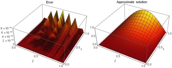
Figure 1. The absolute errors and the approximate solution of Example 1.

Table 3. The $L^{\infty }$ errors of Example 1.

$\mathfrak{L}$	1	3	5	7	9	11
${\beta }_1=0.2,{\beta }_2=0.7$	$1.92567\times {10}^{-1}$	$2.58938\times {10}^{-3}$	$2.56082\times {10}^{-5}$	$1.17456\times {10}^{-7}$	$5.32208\times {10}^{-10}$	$6.13136\times {10}^{-11}$
CPU time	6.798	24.03	57.173	118.672	233.609	379.548

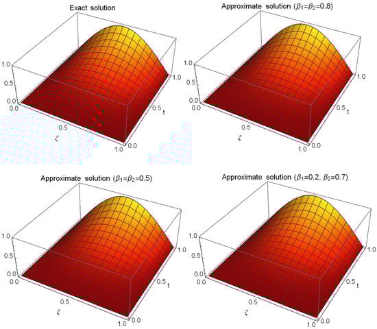
Figure 2. Comparison of exact and approximate solutions at different values of ${\beta }_1$ and ${\beta }_2$ for Example 1.

Table 4. Comparison of $L^2$ and $L^{\infty }$ errors for Example 2.

		${\mathit{L}}^2$ Error		${\mathit{L}}^{\mathit{\infty }}$ Error
${\mathit{\beta }}_{\mathbf{1}}$	${\mathit{\beta }}_{\mathbf{2}}$	Technique in [31]$(\mathit{n}=\mathbf{3},\mathit{m}=\mathbf{70})$	Proposed Technique ($\mathfrak{L}=\mathbf{2}$)	Technique in [31]$(\mathit{n}=\mathbf{3},\mathit{m}=\mathbf{70})$	Proposed Technique ($\mathfrak{L}=\mathbf{2}$)
0.5	0.5	$5.33\times {10}^{-11}$	$4.46221\times {10}^{-19}$	$7.54\times {10}^{-12}$	$8.67362\times {10}^{-18}$
0.8	0.8	$6.21\times {10}^{-11}$	$1.08291\times {10}^{-18}$	$8.33\times {10}^{-12}$	$1.56125\times {10}^{-17}$
0.1	0.9	$3.07\times {10}^{-11}$	$7.99449\times {10}^{-17}$	$5.00\times {10}^{-12}$	$1.11022\times {10}^{-16}$

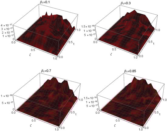
Figure 3. The absolute errors of Example 2.

Table 5. The $L^{\infty }$ errors of Example 3.

$\mathfrak{L}$	2	4	6	8	10
${\beta }_1={\beta }_2=0.4$	$1.22326\times {10}^{-4}$	$1.54893\times {10}^{-7}$	$9.15736\times {10}^{-11}$	$3.44615\times {10}^{-11}$	$3.05118\times {10}^{-11}$
CPU time	15.546	38.579	70.641	122.579	200.514
${\beta }_1={\beta }_2=0.8$	$1.21171\times {10}^{-4}$	$1.54073\times {10}^{-7}$	$8.97306\times {10}^{-11}$	$4.58227\times {10}^{-11}$	$3.01577\times {10}^{-11}$
CPU time	15.102	38.217	70.138	123.225	201.302

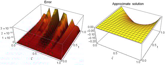
Figure 4. The absolute errors and the approximate solution of Example 3.

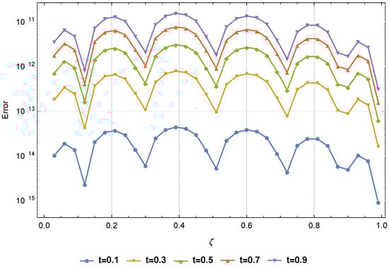
Figure 5. The absolute errors of Example 3.

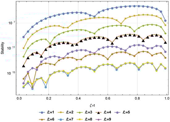
Figure 6. Stability $|{\mathcal{X}}^{\mathfrak{L}+1}(\zeta ,t)-{\mathcal{X}}^{\mathfrak{L}}(\zeta ,t)|$ at $\zeta =t$ for Example 3.

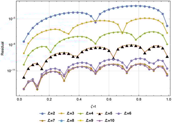
Figure 7. $|R^{\mathfrak{L}}(\zeta ,t)|$ at $\zeta =t$ for Example 3.

Remark 8. 

We want to mention that the advantages of the PGT can be summarized as follows:

• Using the proposed technique allows us to take a few terms of the retained modes and obtain approximations with high precision when compared to the sinc–Bernoulli collocation method [31].
• Compared to numerical techniques that use Chebyshev polynomials, such as the collocation method, which leads to ill-conditioning near $\zeta =0$ and $\zeta =1$, our numerical approach avoids this problem.
• Our proposed technique is simpler to implement compared to wavelet techniques.

7. Conclusions

In this work, a numerical framework was developed for solving the TFCP. We used the modified sets of shifted ($\mathsf{LPs}$) to express the resulting approximate solutions by applying the PGT. The use of these basis functions leads to high accuracy with relatively low polynomial degrees. Numerical simulations with various test problems, including those with known exact solutions, demonstrated that the proposed method significantly improves accuracy and efficiency. We expect that the suggested procedure can be extended to treat other types of DEs in future studies.

References

- Atanackovic, T.M.; Pilipovic, S.; Stankovic, B.; Zorica, D. Fractional Calculus with Applications in Mechanics: Vibrations and Diffusion Processes; Wiley: Hoboken, NJ, USA, 2014. [Google Scholar]
- Kilbas, A.A.; Srivastava, H.M.; Trujillo, J.J. Theory and Applications of Fractional Differential Equations; Elsevier: Amsterdam, The Netherlands, 2006; Volume 204. [Google Scholar]
- Yang, Y.; Huang, Y.; Zhou, Y. Numerical simulation of time fractional cable equations and convergence analysis. Numer. Methods Partial Differ. Equ. 2018, 34, 1556–1576. [Google Scholar] [CrossRef]
- Kosari, S.; Xu, P.; Shafi, J.; Derakhshan, M. An efficient hybrid numerical approach for solving two-dimensional fractional cable model involving time-fractional operator of distributed order with error analysis. Numer. Algorithms 2025, 99, 1269–1288. [Google Scholar] [CrossRef]
- Atta, A.G. Two spectral Gegenbauer methods for solving linear and nonlinear time fractional cable problems. Int. J. Mod. Phys. C 2024, 35, 2450070. [Google Scholar] [CrossRef]
- Salama, F.M. On numerical simulations of variable-order fractional cable equation arising in neuronal dynamics. Fractal Fract. 2024, 8, 282. [Google Scholar] [CrossRef]
- Zheng, S.; Lou, Y.; Shen, S.; Lu, J. Numerical investigation of fractal oscillator for a pendulum with a rolling wheel. Fractals 2025, 33, 2550077. [Google Scholar] [CrossRef]
- Zheng, S.; Chen, L.; Lu, J. Numerical analysis of a fractional micro/nanobeam-based micro-electromechanical system. Fractals 2025, 33, 25500288. [Google Scholar] [CrossRef]
- Chen, B.; Lu, J.; Chen, L. Numerical investigation of a fractal oscillator arising from the microbeams-based microelectromechanical system. Alex. Eng. J. 2025, 126, 53–59. [Google Scholar] [CrossRef]
- Abdelhakem, M.; Abdelhamied, D.; El-Kady, M.; Youssri, Y.H. Two modified shifted Chebyshev–Galerkin operational matrix methods for even-order partial boundary value problems. Bound. Value Probl. 2025, 2025, 34. [Google Scholar] [CrossRef]
- Youssri, Y.H.; Atta, A.G. Optimal third-kind Chebyshev collocation algorithm for solving beam-type micro- and nanoscale BVPs. J. Math. Model. 2025, 13, 841–856. [Google Scholar] [CrossRef]
- Abd-Elhameed, W.M.; Abdelkawy, M.A.; Alqubori, O.M.; Atta, A.G. An accurate tau-based spectral algorithm for the time fractional bioheat transfer model. Bound. Value Probl. 2025, 2025, 124. [Google Scholar] [CrossRef]
- Salamaa, M.H.; Zedan, H.A.; Abd-Elhameed, W.; Youssri, Y.H. Galerkin method with modified shifted Lucas polynomials for solving the 2D Poisson equation. J. Comput. Appl. Mech. 2025, 56, 737–775. [Google Scholar] [CrossRef]
- Taema, M.; Dagher, M.; Youssri, Y. Spectral collocation method via Fermat polynomials for Fredholm–Volterra integral equations with singular kernels and fractional differential equations. J. Math. 2025, 14, 481–492. [Google Scholar]
- Abd-Elhameed, W.M.; Youssri, Y.H.; Doha, E.H. A novel operational matrix method based on shifted Legendre polynomials for solving second-order boundary value problems involving singular, singularly perturbed and Bratu-type equations. Math. Sci. 2015, 9, 93–102. [Google Scholar] [CrossRef]
- Abd-Elhameed, W.M.; Youssri, Y.H. Explicit shifted second-kind Chebyshev spectral treatment for fractional Riccati differential equation. Comput. Model. Eng. Sci. 2019, 121, 1029–1049. [Google Scholar] [CrossRef]
- Bhrawy, A.H.; Abd-Elhameed, W.M. New algorithm for the numerical solutions of nonlinear third-order differential equations using Jacobi-Gauss collocation method. Math. Probl. Eng. 2011, 2011, 837218. [Google Scholar] [CrossRef]
- Youssri, Y.H.; Abd-Elhameed, W.M.; Abdelhakem, M. A robust spectral treatment of a class of initial value problems using modified Chebyshev polynomials. Math. Methods Appl. Sci. 2021, 44, 9224–9236. [Google Scholar] [CrossRef]
- Cui, T.; Xu, C. Müntz Legendre polynomials: Approximation properties and applications. Math. Comput. 2025, 94, 1377–1410. [Google Scholar] [CrossRef]
- Sahabi, M.; Cherati, A.Y. Numerical solutions for fractional optimal control problems using Müntz–Legendre polynomials. J. Mahani Math. Res. Cent. 2025, 14, 189–217. [Google Scholar] [CrossRef]
- Sakar, M.G.; Saldır, O.; Ata, A. Numerical solution of fractional-order multi-point boundary value problems using reproducing kernel method with shifted Legendre polynomials. Z. Angew. Math. Phys. 2025, 76, 141. [Google Scholar] [CrossRef]
- Wu, M.; Zhou, J.; Guan, C.; Niu, J. A numerical method using Legendre polynomials for solving two-point interface problems. AIMS Math. 2025, 10, 7891–7905. [Google Scholar] [CrossRef]
- Heydari, M.H.; Atangana, A.; Avazzadeh, Z. Numerical solution of nonlinear fractal–fractional optimal control problems by Legendre polynomials. Math. Methods Appl. Sci. 2021, 44, 2952–2963. [Google Scholar] [CrossRef]
- Khan, N.A.; Sulaiman, M.; Kumam, P.; Alarfaj, F.K. Application of Legendre polynomials based neural networks for the analysis of heat and mass transfer of a non-Newtonian fluid in a porous channel. Adv. Contin. Discret. Model. 2022, 2022, 7. [Google Scholar] [CrossRef]
- Cao, J.; Chen, Y.; Wang, Y.; Zhang, H. Numerical analysis of nonlinear variable fractional viscoelastic arch based on shifted Legendre polynomials. Math. Methods Appl. Sci. 2021, 44, 8798–8813. [Google Scholar] [CrossRef]
- Sohel, M.N.; Islam, M.S.; Islam, M.S.; Kamrujjaman, M. Galerkin method and its residual correction with modified Legendre polynomials. Contemp. Math. 2022, 3, 188–202. [Google Scholar] [CrossRef]
- Hasan, N.N.; Mohammad, A.J. Nonpolynomial spline method for solving linear fractional differential equations. Int. J. Psychosoc. Rehabil. 2020, 24, 3819–3827. [Google Scholar] [CrossRef]
- Hamasalh, F.K.; Headayat, M.A. The applications of non-polynomial spline to the numerical solution for fractional differential equations. AIP Conf. Proc. 2021, 2334, 060014. [Google Scholar] [CrossRef]
- Vivas-Cortez, M.; Yousif, M.A.; Mahmood, B.A.; Mohammed, P.O.; Chorfi, N.; Lupas, A.A. High-accuracy solutions to the time-fractional KdV–Burgers equation using rational non-polynomial splines. Symmetry 2024, 17, 16. [Google Scholar] [CrossRef]
- Yousif, M.A.; Agarwal, R.P.; Mohammed, P.O.; Lupas, A.A.; Jan, R.; Chorfi, N. Advanced methods for conformable time-fractional differential equations: Logarithmic non-polynomial splines. Axioms 2024, 13, 551. [Google Scholar] [CrossRef]
- Moshtaghi, N.; Saadatmandi, A. Numerical solution of time fractional cable equation via the sinc–Bernoulli collocation method. J. Appl. Comput. Mech. 2021, 7, 1916–1924. [Google Scholar] [CrossRef]
- Podlubny, I. Fractional Differential Equations: An Introduction to Fractional Derivatives, Fractional Differential Equations, Methods of Their Solution and Some of Their Applications; Elsevier: Amsterdam, The Netherlands, 1998; Volume 198. [Google Scholar]
- Napoli, A.; Abd-Elhameed, W.M. Numerical solution of eighth-order boundary value problems by using Legendre polynomials. Int. J. Comput. Methods 2018, 15, 1750083. [Google Scholar] [CrossRef]
- Alzahrani, S.S.; Alanazi, A.A.; Atta, A.G. A modified collocation technique for addressing the time-fractional FitzHugh–Nagumo differential equation with shifted Legendre polynomials. Symmetry 2025, 17, 1468. [Google Scholar] [CrossRef]
Disclaimer/Publisher’s Note: The statements, opinions and data contained in all publications are solely those of the individual author(s) and contributor(s) and not of MDPI and/or the editor(s). MDPI and/or the editor(s) disclaim responsibility for any injury to people or property resulting from any ideas, methods, instructions or products referred to in the content. |
© 2025 by the authors. Licensee MDPI, Basel, Switzerland. This article is an open access article distributed under the terms and conditions of the Creative Commons Attribution (CC BY) license (https://creativecommons.org/licenses/by/4.0/).