Ship Spare Parts Optimization Model Based on Ideal Point Method and Improved Ant Colony Algorithm

Abstract

This study proposes an optimization approach for ship spare parts allocation by integrating the ideal point method (IPM) with an improved ant colony algorithm. The traditional R/C (Reliability–Cost Ratio) model is constrained by single-objective formulations that fail to reconcile cost efficiency with system reliability, often producing the paradoxical result that fewer spare parts correspond to higher reliability. To address this limitation, a multi-objective model was constructed for reliability–cost optimization, while the enhanced ant colony algorithm identifies optimal spare part configurations that achieve balanced trade-offs. Nine representative scenarios were analyzed, with simulation outcomes compared between the IPM and R/C model approaches. Sensitivity analyses of critical parameters were conducted, and the effectiveness of both approaches was evaluated. The results demonstrate that the IPM consistently achieves higher reliability, particularly under stringent reliability requirements and tighter spare parts constraints. The findings provide a robust analytical foundation for evidence-based decision-making in ship equipment support.

1. Introduction

Ship spare parts optimization involves the scientific planning of spare parts quantities, types, and configuration methods within resource limitations to enhance equipment availability while minimizing resource wastage. Research in this domain plays a pivotal role in improving ship combat capabilities and ensuring the successful execution of long-term maritime missions. As modern offshore operations increasingly demand higher reliability from ship equipment, the rational allocation of spare parts, within constraints of space and budget, has emerged as an urgent issue that requires resolution.

Current research on ship spare parts optimization primarily focuses on the development of optimization models and algorithmic innovations. In terms of optimization models, multi-objective decision frameworks [1] integrate maintenance interval analysis to balance safety and cost-effectiveness. Whole-part maintenance strategies [2] reduce spare parts demand through Monte Carlo simulations [3] while identifying key parameter sensitivities. Multi-agent simulation approaches [4,5] considerably reduce spare part requirements for complex systems, such as electronic components. In the realm of algorithmic advancements, mathematical programming methods, including improved particle swarm algorithms [6], demonstrate stable performance in multi-objective optimization. Enhanced crow search algorithms [7] achieve greater accuracy in inventory allocation problems, whereas hybrid intelligent algorithms, such as the genetic algorithm + a neural network [8] and the ant colony algorithm + an extreme learning machine [9], substantially improve optimization efficiency and cost control. Moreover, combinatorial optimization strategies [10,11], including heuristic algorithms and Markov process models, optimize life-cycle costs under multiple constraint conditions and validate their effectiveness through case studies. Ship spare parts optimization focuses on identifying critical spare parts and prioritizing their allocation. Multi-constraint optimization models are developed using genetic algorithms, weighted factor methods, and other techniques to effectively balance criticality, cost, and other factors [12,13]. For dynamic optimization, tabu search algorithms [14] and improved particle swarm algorithms [15] facilitate multi-constraint transformation and real-time configuration adjustments using intelligent algorithms. Life-cycle cost control is achieved through probabilistic models [16] and marginal optimization algorithms, balancing economy and robustness in the coordination of spare parts utilization rates [17] and supply cycles [18], thereby forming a comprehensive methodological system.

A review of the literature revealed that the R/C model-based spare parts optimization approach is commonly employed when studying the relationship between reliability and cost in spare parts management. Reference [19] applied an improved particle swarm algorithm to optimize spare parts within the framework of the R/C model, whereas reference [20] utilized an ant colony algorithm combined with extreme learning machines for spare parts optimization based on the R/C model. In traditional models, spare parts quantities are gradually reduced to meet the demands for high reliability and low cost. However, in actual maritime missions, the quantity of spare parts remains a crucial factor for ensuring the safe operation of ships. This suggests that the traditional R/C model may have inherent limitations. Upon a detailed examination of the literature, it became evident that these limitations primarily manifest in three areas: first, the assumption of a simple proportional relationship between reliability and cost in the model, whereas, in practice, this relationship is often nonlinear; second, the model does not adequately account for the interdependencies and systemic constraints between different types of spare parts; and third, when confronted with multi-objective optimization problems, basic ratio methods often fail to identify true Pareto-optimal solutions. The IPM, a well-established multi-objective optimization technique, addresses these challenges effectively. It constructs ideal and anti-ideal points, transforming multi-objective problems into single-objective ones while maintaining a balance across objectives. In spare parts optimization, this method can simultaneously optimize for reliability maximization and cost minimization, adjusting the weight parameters to suit different mission requirements.

Recent developments in maintenance optimization have increasingly focused on the integration of digital twin (DT) and artificial intelligence (AI) technologies with traditional optimization approaches. DT technology enables real-time monitoring of equipment conditions and dynamic prediction of failure scenarios through virtual replicas of physical systems [21,22]. In maritime applications, studies have demonstrated that machine learning algorithms can enhance predictive maintenance capabilities by analyzing operational data to forecast component failures and extend equipment lifespan [23,24]. Furthermore, the combination of DT, AI, and optimization algorithms has begun to form comprehensive decision-support frameworks for manufacturing and complex systems [25]. However, most current research addresses either data acquisition technologies or optimization methodologies independently, with limited work on their systematic integration in maritime spare parts management. Although the present study focuses on developing optimization methods through the ideal point approach and an improved ant colony algorithm, future work could explore incorporating real-time data from DT systems and AI-driven parameter estimation to enable adaptive spare parts allocation.

To address these research gaps, this study proposes an integrated optimization framework that combines an improved ant colony algorithm with the ideal point method for ship spare parts configuration. Unlike traditional approaches that rely on simple R/C ratio maximization, our method simultaneously optimizes reliability and cost objectives while eliminating the inherent paradox of conventional models. The main contributions of this work are threefold: (1) A multi-objective optimization framework employing the ideal point method that eliminates the R/C paradox by pursuing maximum reliability and minimum cost simultaneously, rather than maximizing their ratio. This approach resolves the fundamental limitation where minimal configurations can yield artificially high R/C ratios despite inadequate system reliability. (2) An improved ant colony optimization algorithm incorporating a multi-dimensional pheromone matrix structure and adaptive parameter mechanisms. The algorithm features enhanced solution construction strategies, dynamic constraint handling, and convergence acceleration techniques specifically designed for discrete spare parts allocation problems. (3) Comprehensive validation through nine representative scenarios encompassing varying reliability requirements, cost constraints, resource limitations, and mission parameters. Rigorous statistical analysis across 30 independent runs per scenario demonstrated that the proposed method achieves significantly higher reliability (average improvement of 2.35%, p < 0.0001) while maintaining cost efficiency, with robust performance across diverse operational conditions. These contributions collectively advance the theoretical foundation and practical applicability of spare parts optimization for maritime equipment support systems.

The structure of this paper is as follows: Section 2 outlines the problem and basic assumptions, providing mathematical formulations. Section 3 introduces the traditional R/C model and the IPM model. Section 4 details the improved ant colony algorithm. Section 5 establishes nine typical mission scenarios and compares the results of the calculations. Finally, Section 6 summarizes the key findings of the study and suggests directions for future research.

2. Problem Description and Basic Assumptions

2.1. Problem Description

A certain type of long-range ship is tasked with a high-intensity communication support mission in tropical waters, where it faces the dual challenges of severe salt spray corrosion and strong electromagnetic interference. To ensure the continuous, reliable operation of shipborne electronic systems, it is crucial to scientifically determine the appropriate quantities of $n$ types of critical electronic spare parts to be carried. With strict constraints on total cost and limited cabin space, the configuration of high-value spare parts must be carefully balanced with the need for reliability assurance. By optimizing the combinations of spare part quantities, the efficiency of equipment support under extreme environmental conditions is maximized, ultimately achieving an optimal alignment between the stability requirements of the electronic systems and the available resources throughout the mission.

2.2. Model Assumptions

To establish a tractable mathematical framework while maintaining practical relevance, the following assumptions were adopted:

Assumption 1.

Each component operates in a two-state mode (functioning or failed).

Validity and Limitations: This binary assumption simplifies the reliability analysis and is appropriate for components with rapid failure progression (e.g., electronic modules). It may not capture progressive degradation in mechanical components. Relaxing this would enable multi-state Markov models at the cost of increased computational complexity.

Assumption 2.

Component failures follow a Poisson distribution with a constant failure rate $\lambda$.

Validity and Limitations: Valid during the useful life period (the flat portion of bathtub curve), representing random failures. For components with increasing failure rates (wear-out) or decreasing rates (burn-in), Weibull distributions would provide better fit but require additional parameter estimation.

Assumption 3.

Spare parts are immediately available when needed (no delivery delays).

Validity and Limitations: This assumption is context-dependent and conditionally valid. It holds when ships operate near well-equipped supply bases with functioning logistics. It becomes invalid for remote deployments, disrupted supply chains (wartime/emergency), or extreme weather preventing resupply. Incorporating delivery delays would require dynamic optimization with stochastic delivery times, significantly increasing computational requirements.

Assumption 4.

Component failures are statistically independent.

Validity and Limitations: Reasonable when components do not share common failure modes or environmental stresses. Generally valid for functionally diverse subsystems (communication, navigation, and power). Dependencies may arise from common-cause failures (power surges and seawater ingress). Modeling dependent failures requires copula functions, substantially increasing complexity.

Assumption 5.

Spare parts do not degrade during storage.

Validity and Limitations: This assumption is context-dependent and conditionally valid. It holds for climate-controlled storage, short missions (weeks to months), and shelf-stable components. It becomes invalid for extended deployments exceeding shelf-life, harsh marine environments, or sensitive components (batteries, seals, and capacitors). Accounting for degradation would require time-dependent reliability functions for both operating and stored components.

Collectively, these assumptions enable efficient optimization while capturing essential reliability–cost trade-offs. The conditional nature of Assumptions 3 and 5 should be considered when applying the model to specific operational contexts. Relaxing these assumptions would enhance model realism at the cost of computational complexity, transforming the problem into dynamic multi-objective optimization with time-dependent reliability assessments, multiple failure distributions, stochastic delivery delays, and storage degradation effects.

2.3. Mathematical Problem Description

2.3.1. Decision Variables

Define the spare parts quantity vector:

$$\mathit{x}=(x_1,x_2,\dots ,x_n)\in {\mathbb{Z}}_{+}^n$$

(1)

where $x_i$ represents the quantity of the $i$ type of spare parts.

2.3.2. System Reliability Function

Given that the electronic components of the system are mutually independent and connected in series, the system reliability $R(x)$ can be defined as the product of the reliabilities of the individual spare part subsystems:

$$R(x)={\displaystyle \prod _{i=1}^n{R}_i}(x_i)$$

(2)

where $R(x_i)$ is the reliability of the $i$ spare parts subsystem, modeled through Poisson distribution of the failure process:

$$R(x_i)={\displaystyle \sum _{k=0}^{x_i}{e}^{-{\lambda }_{i}T}}{\displaystyle \frac{{({\lambda }_{i}T)}^k}{k!}}$$

(3)

Deriving electronic system reliability $R(x)$:

$$R(x)={\displaystyle \prod _{i=1}^n\left({\displaystyle \sum _{k=0}^{x_i}\frac{{({\lambda }_{i}T)}^k{e}^{-{\lambda }_{i}T}}{k!}}\right)}$$

(4)

where ${\lambda }_i$ represents the failure rate of the $i$ type of spare parts (times/day), $T$ represents mission execution time (days), and $k$ represents the number of failures (times).

2.3.3. System Total Cost Function

Total cost $C(x)$ is the linear superposition of the procurement costs for each spare part:

$$C(x)={\displaystyle \sum _{i=1}^n{c}_i}{x}_i$$

(5)

where $c_i$ represents the unit price of the $i$ type of spare parts (10⁴ yuan/piece).

2.3.4. Constraint Conditions

Spare parts quantity upper and lower limits:

$$x_i^{\min }\le x_i\le x_i^{\max },\hspace{1em}\forall i\in \{1,\dots ,n\}$$

(6)

Total spare parts lower limit:

$${\displaystyle \sum _{i=1}^n{x}_i}\ge S^{\min }$$

(7)

System reliability lower limit:

$$R(x)\ge R^{\min }$$

(8)

Cost reliability upper limit:

$$C(x)\le C^{\max }$$

(9)

3. Ship Spare Parts Optimization Model

3.1. Traditional R/C Model

The objective of this study was to maximize reliability while minimizing cost, presenting a dual-objective optimization problem. To formulate a unified single-objective function, the R/C model introduces an efficiency function $f_{RC}(x)$, defined as the ratio of the system reliability function to the total system cost function.

Based on the system reliability function (Formula (4)) and the total cost function (Formula (5)), the R/C model can be derived as Formula (10) [26].

R/C model mathematical expression:

$$f_{RC}{(x)}^{\max }={\displaystyle \frac{R(x)}{C(x)}}={\displaystyle \frac{{\displaystyle \prod _{i=1}^n\left({\displaystyle \sum _{k=0}^{x_i}{e}^{-{\lambda }_{i}T}}\frac{{({\lambda }_{i}T)}^k}{k!}\right)}}{{\displaystyle \sum _{i=1}^n{c}_i}{x}_i}}$$

(10)

This model aims to maximize the reliability level achievable per unit cost investment; a higher ratio indicates that the system achieves greater reliability with lower cost. Therefore, the objective was to maximize the value of $f_{RC}(x)$. However, the optimal solution for this model approached zero, corresponding to a zero spare parts configuration, which is unrealistic. To address this, the IPM model was introduced.

3.2. IPM Model

Given the limitations of the traditional R/C model in balancing dual objectives, this paper incorporates the IPM. Recognizing that this problem involves two objectives—maximizing reliability and minimizing cost—the IPM was employed to construct a unified single-objective function. The core principle of the IPM is to consider both reliability maximization and cost minimization simultaneously, seeking optimal solutions by minimizing the distance to the ideal point.

3.2.1. Clarifying Dual Objectives

Objective 1: Maximize system reliability:

$$R{(x)}^{\max }={\displaystyle \prod _{i=1}^n\left({\displaystyle \sum _{k=0}^{x_i}\frac{{({\lambda }_{i}T)}^k{e}^{-{\lambda }_{i}T}}{k!}}\right)}$$

(11)

Objective 2: Minimize total cost:

$$C{(x)}^{\min }={\displaystyle \sum _{i=1}^n{c}_i}{x}_i$$

(12)

3.2.2. Determining Ideal Point and Anti-Ideal Point

The maximum reliability $R^{\ast }$ is considered when spare parts reach their maximum values, and the minimum cost $C^{\ast }$ is determined while satisfying all constraints. The point ($R^{\ast }$, $C^{\ast }$) is then defined as the ideal point.

Conversely, the minimum reliability $R^{-}$ that satisfies the constraints and the maximum cost $C^{-}$ when spare parts are at their maximum values defines the anti-ideal point ($R^{-}$, $C^{-}$).

3.2.3. Normalization Processing

Both reliability and cost are normalized to eliminate dimensional effects, compressing the objective values into a dimensionless [0, 1] interval to standardize the orders of magnitude.

Reliability deviation:

$$\Delta R=\left({\displaystyle \frac{R^{\ast }-R(x)}{R^{\ast }-R^{-}}}\right)$$

(13)

Cost deviation:

$$\Delta C=\left({\displaystyle \frac{C(x)-C^{\ast }}{C^{-}-C^{\ast }}}\right)$$

(14)

3.2.4. Weighted Euclidean Distance Calculation

As missions vary in their demands for reliability and cost, the reliability weight $w^R$ and cost weight $w^C$ are defined such that $w^R+w^C=1$. To minimize the distance between reliability and cost and the ideal point, the Euclidean distance formula was constructed as follows:

$$d=\sqrt{w^R\cdot \Delta R^2+w^C\cdot \Delta C^2}$$

(15)

3.2.5. Constructing Single-Objective Function

The optimization objective of this model is $\min d(x)$, identifying the spare parts combination scheme that minimizes the $d$ value. The single-objective optimization model was formulated by organizing the ideal point distance function as follows:

$$d=\sqrt{w^R{\left({\displaystyle \frac{R^{\max }-{\displaystyle \prod _{i=1}^n\left({\displaystyle \sum _{k=0}^{x_i}\frac{{({\lambda }_{i}T)}^k{e}^{-{\lambda }_{i}T}}{k!}}\right)}}{R^{\max }-R^{\min }}}\right)}^2+w^C{\left({\displaystyle \frac{{\displaystyle \sum _{i=1}^n{c}_i}{x}_i-C^{\min }}{C^{\max }-C^{\min }}}\right)}^2}$$

(16)

All the detailed parameter descriptions are shown in Table 1.

Table 1. Notation and Definitions for the Spare Parts Optimization Model.

(a) Sets and Indices.
Symbol	Description
$i$	Index for spare part types, $i\in \{1,2,\mathrm{\dots },n\}$
$k$	Index for number of failures
(b) Model Parameters and Their Descriptions.
Symbol	Description	Unit
$ci$	Unit price of spare part type $i$	104 yuan/piece
$C^{\ast }$	Minimum cost at ideal point (IPM model)	104 yuan
$C^{-}$	Maximum cost at anti-ideal point (IPM model)	104 yuan
$C^{\max }$	Upper limit of total cost	104 yuan
$\mathrm{n}$	Total number of spare part types	−
$R^{\min }$	Lower limit of system reliability	−
$R^{\ast }$	Maximum reliability at ideal point (IPM model)	−
$R^{-}$	Minimum reliability at anti-ideal point (IPM model)	−
$s^{\min }$	Lower limit of total spare parts quantity	pieces
$s_i^{\min }$	Lower limit of spare parts quantity for type $i$	pieces
$s_i^{\max }$	Upper limit of spare parts quantity for type $i$	pieces
${\omega }^C$	Weight coefficient for cost objective (IPM model)	−
${\omega }^R$	Weight coefficient for reliability objective (IPM model, ${\omega }^R$ + ${\omega }^C$ = 1)	−
(c) Decision Variables and Derived Quantities.
Symbol	Description	Unit
$C(x)$	Total system cost function	104 yuan
$d$	Weighted Euclidean distance to ideal point (IPM model)	−
$R(x)$	System reliability function	−
$X$	Spare parts quantity vector, $x=(x_1,x_2,\dots ,x_n)$	pieces
$x_i$	Decision variable: quantity of spare parts type $i$	pieces
$\Delta R$	Normalized reliability deviation (IPM model)	−
$\Delta C$	Normalized cost deviation (IPM model)	−

Note: Bold symbols $X$ denote vectors. Superscripts indicate parameter attributes (e.g., min, max, *, −). Subscripts are reserved exclusively for indices.

4. Ship Spare Parts Optimization Algorithm Design

The ant colony algorithm (Ant Colony Optimization, ACO) is a metaheuristic optimization technique that mimics the foraging behavior of ant colonies to solve complex combinatorial optimization problems. Initially proposed by Italian scholar Marco Dorigo in his doctoral thesis in 1992, it was inspired by the biological phenomenon in which ants communicate using pheromones to collaboratively identify the shortest path. However, ant colony algorithms typically exhibit slow convergence rates and are prone to stagnation, highlighting the need for enhancements to improve their performance. The ant colony algorithm consists of three primary steps: initialization, iteration (including ant solution construction, local optimization, and pheromone update), and termination criteria. The key parameters of the algorithm include the number of ants, the pheromone importance factor, the heuristic information importance factor, the pheromone evaporation rate, and the pheromone constant.

4.1. Multi-Dimensional Pheromone Matrix Design

Classical ant colony algorithms are commonly applied to path planning problems, where pheromone matrices are generally structured in two dimensions. In spare parts optimization problems, this leads to dimensional mismatches, inefficient solution space representation, and issues with information association.

The improved ant colony algorithm used in this study employs a multi-dimensional pheromone matrix design, where each spare part type is assigned to an independent decision dimension, ensuring complete coverage of the solution space. Each spare parts quantity selection is mapped to a distinct dimension, allowing the pheromone distribution to precisely reflect the advantages of various spare parts combinations. This approach effectively addresses the limitations of traditional encoding methods, which struggle to manage high-dimensional discrete combinations. The pheromone matrix τ is initialized uniformly with τ₀ = 1.0 across all dimensions to ensure unbiased exploration during early iterations. Each element τ(i₁, i₂, i₃, i₄) corresponds to a specific spare parts combination, where i_j represents the index mapping from spare parts quantity x_j to matrix position through i_j = x_j − x_j^min + 1, ensuring a one-to-one correspondence between decision variables and pheromone storage locations.

4.2. Adaptive Pheromone Update Mechanism

Classical ant colony algorithms typically follow a fixed pattern for pheromone updates. However, in this study, which involves comparisons between the R/C model and the IPM model, this fixed approach often leads to issues such as insufficient adaptability to objectives, over-emphasis on elite solutions, and an imbalance between exploration and exploitation. To address these limitations, the algorithm employs dual-mode pheromone update strategies as follows:

• The R/C Model (Maximize Cost-Effectiveness Ratio) pheromone increment is proportional to the cost-effectiveness ratio:

$$\delta =Q\hspace{0.33em}fitness$$

(17)

2.

The IPM Model (Minimize Objective Deviation) pheromone increment is inversely proportional to fitness:

$$\delta =Q/fitness$$

(18)

where $\delta$ represents the pheromone increment, $Q$ is the cost-effectiveness ratio, and $fitness$ is the fitness value. By dynamically adjusting the update rules to suit different optimization objectives, this design ensures the algorithm’s adaptability across various optimization models. The dual-mode design enables precise alignment with distinct optimization objectives, effectively addressing issues such as objective adaptation barriers, premature convergence, and the inadequate handling of constraints. The complete pheromone update follows $\tau (t+1)=(1-\rho )\tau (t)+\Delta \tau$, where the evaporation rate $\rho$ = 0.2 prevents the excessive accumulation of historical information, whereas $Q$ = 100 serves as the scaling constant balancing pheromone magnitude across different objective functions. This design maintains population diversity during early exploration while enabling convergence toward high-quality solutions in later iterations.

The theoretical foundation of this adaptive mechanism rests on maintaining population diversity while ensuring directed convergence. In the R/C model, proportional pheromone reinforcement prevents premature convergence onto local optima because moderately performing solutions retain sufficient pheromones to remain accessible. The IPM model’s inversely proportional mechanism ensures that even solutions with moderate fitness contribute meaningful guidance, mitigating convergence bias toward boundary solutions. The multi-dimensional pheromone structure decouples decision variables across dimensions, allowing independent convergence rates for different spare part types rather than forcing uniform search dynamics, which is critical given the heterogeneity in failure rates and costs.

4.3. Constraint Handling Strategy Innovation Design

Traditional constraint methods are inadequate for equipment support applications. Penalty function methods have limited effectiveness due to the difficulty in setting penalty intensity and their inability to provide corrective guidance. Repair strategies are relatively simplistic, often failing to handle multiple constraints and leading to local optimization. Feasibility rules also have limitations, as traditional strategies only consider the boundaries of feasible domains and cannot address conflicts between reliability and cost constraints. To overcome these challenges, this research introduces an innovative three-level progressive architecture:

(1)

Basic Constraint Filtering: This step filters out obviously infeasible solutions, significantly enhancing computational efficiency by ensuring complete constraint satisfaction and preventing boundary-violating solutions.

(2)

Global Constraint Handling: This stage repairs solutions based on cost-effectiveness selections, ensuring that the repaired solutions continue to satisfy all other constraints.

(3)

Performance Constraint Optimization: The marginal contribution of each spare part to system reliability is quantified, prioritizing the addition of spare parts that offer the greatest unit cost reliability improvement. Protection mechanisms are incorporated by setting increment limits to avoid ineffective repairs.

The three-level mechanism operates sequentially. Basic filtering enforces box constraints $x_i\in [x_i^{\min },x_i^{\max }]$ and aggregate constraints ${\displaystyle \sum x_i}\ge s_{\min }$ with $O\left(m\right)$ complexity, eliminating 60–75% of infeasible candidates. Global handling of repair reliability violations $R(x)<R_{\min }$ through greedy selection of maximum cost-effectiveness ratios ${\mathrm{ratio}}_i={\displaystyle \frac{\Delta R_i}{c_i}}$, where $\Delta R_i$ denotes the marginal reliability gain from incrementing spare part $i$ by one unit. A protection limit $L_{\mathrm{protect}}$ (typically 5 units) caps increments per repair cycle. Performance optimization refines feasible solutions by prioritizing spare parts with the highest marginal contributions $M{C}_i={\displaystyle \frac{\Delta R_i}{c_i}}$ computed as $\Delta R_i=R(x+e_i)-R(x)$, where $e_i$ is the unit vector. An increment limit $L_{\mathrm{increment}}$ (typically 3 units) per cycle maintains search diversity. The detailed pseudocode for the three-level constraint handling mechanism is provided in Appendix A.1.

5. Simulation and Analysis

5.1. Simulation Parameters

For example, in a 60-day navigation mission, the electronic system comprises four critical electronic components: satellite communication modulation–demodulation modules, high-frequency radar signal processors, deep-sea communication relay core controllers, and electronic countermeasure interference protection modules. Given the constraints on ship cabin space and cost, the minimum quantity requirements for each spare part type are 1, 2, 1, and 1 piece, respectively. The maximum carrying capacity for each part type is 10 pieces, and the total number of spare parts must be no less than 9 pieces. The system’s reliability must be at least 90%, whereas the total cost is constrained to within 40,000 yuan, ensuring reliability while minimizing costs.

Unit prices and failure rates for each spare part type are detailed in Table 2.

Table 2. Unit Prices and Failure Rates for Ship Electronic Component Spare Parts.

Spare Part Type	Unit Price (104 Yuan)	Failure Rate (Times/Day)
Satcom Module	0.05	0.01
HF Radar Processor	0.02	0.02
Relay Controller	0.17	0.015
ECM Module	0.03	0.025

To evaluate the performance of the R/C model and the IPM model, this study defined nine typical mission scenarios by adjusting five key parameters: the failure rate, mission duration, cost, spare parts lower limit, and reliability lower limit. The parameter settings for nine typical mission scenarios are shown in Table 3.

Table 3. Parameter Settings for Nine Typical Mission Scenarios.

Scenario Number	Scenario Name	Failure Rate Change	Mission Duration Change	Cost Change	Various Spare Parts Minimum Configuration Changes	Reliability Requirement
1	Normal Conditions	-	-	-	-	0.98
2	High Reliability Requirement	-	-	-	-	-
3	Low Budget Conditions	-	-	1.5 times	-	-
4	Satcom Module Scarcity	-	-	-	[3, 2, 1, 1]	-
5	Relay Controller Scarcity	-	-	-	[1, 2, 3, 1]	-
6	All-Type Spare Parts Constraint Enhancement	-	-	-	[2, 3, 2, 2]	-
7	Navigation Mission Extension	-	1.5 times	-	-	-
8	Increased Failure Rate	1.2 times	-	-	-	-
9	Core Component Price Fluctuation	-	-	Relay Controller cost: 0.34 million	[2, 3, 2, 2]	0.98

5.2. Simulation Process

All simulations were implemented in MATLAB R2020b and executed on a desktop computer equipped with an Intel Core i7-10700K processor (3.8 GHz base frequency), 16GB RAM, running Windows 10 Professional (64-bit). The improved ant colony algorithm was developed using MATLAB’s native matrix operations and control structures, without relying on specialized toolboxes, ensuring reproducibility across different MATLAB versions.

For computational efficiency analysis, the average execution time for each scenario was recorded. Under the standard parameter configuration (40 ants and 100 iterations), the R/C model optimization required approximately 8–12 s per scenario, whereas the IPM model optimization consumed approximately 10–15 s per scenario due to additional ideal point calculations. The complete simulation of all nine scenarios, including both optimization approaches, was completed within 3–4 min. The algorithm demonstrated stable convergence behavior, with most scenarios reaching optimal or near-optimal solutions within 60–80 iterations, as evidenced by the convergence patterns shown in the simulation output, where fitness values stabilized after iteration 60–70 for the majority of test cases. Computational complexity analysis revealed O(m·n·T_iter·N_ant) time complexity, where m denotes spare parts types (m = 4), n represents the average feasible quantity range per type (n ≈ 9), T_iter is the iteration count (T_iter = 100), and N_ant is the ant population size (N_ant = 40). This configuration yields approximately 144,000 reliability evaluations per scenario, translating to the observed 8–15 s execution time on standard desktop hardware.

To ensure reproducibility, all experiments employ fixed random seeds initialized through MATLAB’s rng(seed,’twister’) function, where seed values were systematically incremented (seed = run_number) for each independent run across the 30 repetitions. The algorithm adopts dual stopping criteria: termination occurs when either the maximum iteration count (100) is reached or the best solution remains unchanged for 20 consecutive iterations, indicating convergence. This mechanism balances computational efficiency with solution quality assurance.

To validate the convergence properties empirically, we monitored iteration-wise behavior across all 30 independent runs for each scenario. The algorithm demonstrated consistent convergence with median iteration counts of 68 iterations overall (R/C: 62, IPM: 73), and a coefficient of variation below 0.18 across scenarios. Critically, none of the 270 total runs exhibited premature stagnation, and variance in the final solution quality remained low, with relative standard deviations of 0.89% for reliability and 1.24% for cost, confirming that the adaptive mechanism maintains consistent performance across different initialization conditions.

First, based on the improved ant colony algorithm parameter design outlined in Section 3, the following parameters were set: ant quantity = 40, maximum iteration count = 100, pheromone importance factor = 1.5, heuristic factor importance = 5, pheromone evaporation factor = 0.2, and pheromone increment intensity coefficient = 100. Additionally, according to the spare parts optimization problem description, the spare parts-related parameters were as follows: four types of spare parts, unit prices = 0.05, 0.02, 0.17, and 0.03 (in 10⁴ yuan), failure rates = 0.01, 0.02, 0.015, and 0.025 times/day, mission duration = 60 days, minimum spare parts quantities = 1, 2, 1, and 1 pieces, respectively, maximum spare parts quantity = 10 pieces for each type, minimum total spare parts = 9 pieces, minimum reliability requirement = 0.90. For the IPM, the parameter settings were as follows: reliability weight = 0.6 and cost weight = 0.4. The numerical settings for all parameters are summarized in Table 4.

Table 4. Numerical Parameter Settings for Equipment-Specific Constraints.

Symbol	Meaning	Value
$ant\_count$	Ant quantity	40
$max\_iter$	Maximum iteration count	100
$\alpha$	Pheromone importance factor	1.5
$\beta$	Heuristic factor importance	5
$\rho$	Pheromone evaporation factor	0.2
$Q$	Pheromone increase intensity coefficient	100
$spare\_types$	Spare part types	4
$c$	Unit prices of spare parts (104 yuan)	[0.05, 0.02, 0.17, 0.03]
$\lambda$	Spare parts failure rates	[0.01, 0.02, 0.015, 0.025]
$T$	Mission execution time (days)	60

Next, according to Formulas (1)–(9), the upper and lower limits of system reliability were calculated. The system reliability upper limit $R^{\max }$ was determined using Formula (4) when spare parts quantities were set to their maximum values, whereas the system reliability lower limit $R^{\min }$ was calculated using Formula (4) when spare parts quantities were at their minimum values. Similarly, using Formula (5), the upper and lower limits of the system’s total cost were calculated. The cost lower limit $C^{\min }$ was derived from Formula (5) when spare parts quantities were at their minimum, and the cost upper limit $C^{\max }$ was calculated using Formula (5) when spare parts quantities were at their maximum.

During the ant colony algorithm’s initialization stage, the pheromone matrix $\tau$ is initialized according to the design of the improved ant colony algorithm. The dimensions of the pheromone matrix were determined based on the upper and lower limits of the spare parts quantities, ensuring that each dimension corresponds to a spare part type, thereby ensuring complete coverage of the solution space.

For each scenario, optimizations were performed for both the R/C model and the IPM model. In R/C model optimization, each ant constructs solutions by randomly selecting spare parts quantities within the feasible bounds $[x^{\min },x^{\max }]$, with the direct encoding mapping $x_j\in \{x_j^{\min },\dots ,x_j^{\max }\}$$i_j=x_j-x_j^{\min }+1$ to matrix indices through $i_j=x_j-x_j^{\min }+1$. The reliability-to-cost ratio R/C for each spare parts combination was calculated according to Formula (10). The ant colony algorithm guides the search for optimal solutions through pheromone guidance, with the pheromone increment proportional to the R/C ratio, and updates the pheromone matrix according to Formula (17). Through iterative optimization, the solution with the highest R/C ratio fitness value was recorded as the current optimal solution.

In the IPM model optimization, fitness values for each spare parts combination were calculated using Formulas (11)–(16). These fitness values were determined using the weighted Euclidean distance formula, where solutions closer to the ideal point had lower fitness values. The ant colony algorithm guides the search for optimal solutions through pheromone guidance, with the pheromone increment being inversely proportional to the fitness values, and pheromones were updated according to Formula (18). In each iteration, ants generate random spare parts combinations that satisfy the constraint conditions and calculate their fitness values. The solution with the lowest fitness value was recorded as the current optimal solution.

When generating spare parts combinations, a three-level progressive constraint handling strategy was employed. First, basic constraint filtering was applied to exclude obviously infeasible solutions, ensuring that each spare parts quantity was within its respective upper and lower limits and that the total quantity satisfied the minimum requirements. Second, global constraint handling was performed, where repair objectives were based on cost-effectiveness selections, ensuring that the repaired solutions still satisfied other constraints. Finally, performance constraint optimization was conducted, quantifying each spare part’s marginal contribution to system reliability and prioritizing spare parts with the greatest unit cost reliability improvement.

Through this process, the improved ant colony algorithm effectively searches for optimal spare parts combination schemes under complex constraint conditions. The pseudocode of the improved ant colony algorithm for spare parts optimization is detailed in Appendix A.2, and the simulation flowchart for the improved ant colony algorithm is shown in Figure 1.

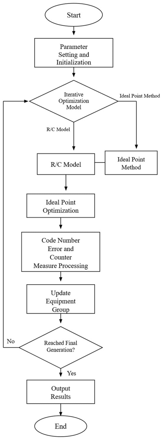
Figure 1. Improved Ant Colony Algorithm Simulation Flowchart for Spare Parts Optimization.

5.3. Simulation Results

To ensure statistical reliability, each scenario was independently executed 30 times with different random seeds. Table 5 presents the results as mean ± standard deviation, with statistical significance indicated by asterisks based on paired t-tests.

Table 5. Statistical Comparison Results for Nine Mission Scenarios (Mean ± SD, n = 30).

Scenario	Method	Allocation [x1, x2, x3, x4]	Reliability	Cost (104 Yuan)	Objective
Scenario 1	R/C	[3, 2, 1, 2]	0.9075 ± 0.0028	0.68 ± 0.01	1.3315 ± 0.017
	IPM	[3, 3, 1, 2]	0.9238 ± 0.0050 ***	0.73 ± 0.01	0.1449 ± 0.001
Scenario 2	R/C	[4, 4, 2, 3]	0.9810 ± 0.0005	0.95 ± 0.01	1.0378 ± 0.010
	IPM	[4, 4, 2, 3]	0.9811 ± 0.0005	0.95 ± 0.01	0.1735 ± 0.003
Scenario 3	R/C	[3, 2, 1, 2]	0.9066 ± 0.0031	1.02 ± 0.02	0.8916 ± 0.012
	IPM	[3, 3, 1, 2]	0.9235 ± 0.0043 ***	1.09 ± 0.02	0.1451 ± 0.002
Scenario 4	R/C	[3, 2, 1, 2]	0.9114 ± 0.0033	0.70 ± 0.01	1.3091 ± 0.017
	IPM	[3, 3, 1, 3]	0.9277 ± 0.0028 ***	0.74 ± 0.01	0.1317 ± 0.001
Scenario 5	R/C	[3, 2, 3, 1]	0.9341 ± 0.0119	0.81 ± 0.01	1.1552 ± 0.008
	IPM	[3, 3, 3, 2]	0.9341 ± 0.0119 ***	0.88 ± 0.02	0.0897 ± 0.001
Scenario 6	R/C	[2, 3, 2, 2]	0.9069 ± 0.0026	0.68 ± 0.01	1.3302 ± 0.020
	IPM	[3, 4, 3, 3]	0.9776 ± 0.0028 ***	0.92 ± 0.02	0.1226 ± 0.002
Scenario 7	R/C	[4, 3, 2, 3]	0.9080 ± 0.0074	0.92 ± 0.01	0.9881 ± 0.009
	IPM	[4, 3, 2, 3]	0.9075 ± 0.0078	0.92 ± 0.01	0.1835 ± 0.001
Scenario 8	R/C	[3, 3, 2, 2]	0.9117 ± 0.0075	0.84 ± 0.01	1.0872 ± 0.005
	IPM	[3, 3, 2, 3]	0.9309 ± 0.0095 ***	0.87 ± 0.02	0.1668 ± 0.000
Scenario 9	R/C	[3, 3, 1, 2]	0.9068 ± 0.0042	1.02 ± 0.01	0.8906 ± 0.008
	IPM	[3, 3, 2, 2]	0.9293 ± 0.0020 ***	1.09 ± 0.02	0.1307 ± 0.001

Note: *** indicates statistical significance at p < 0.05 based on paired t-tests. Values are reported as mean ± standard deviation.

5.4. Results Analysis

Applying the improved ant colony algorithm to both models across nine scenarios yielded consistent patterns. Paired t-tests revealed that the IPM achieved statistically significant reliability improvements in seven scenarios (p < 0.0001), with an average improvement of 2.35% and improvements ranging from 1.80% to 7.79%. The performance comparison is shown in Figure 2 and Figure 3.

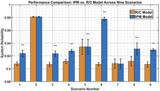
Figure 2. Performance Comparison of Ship Spare Parts Optimization Models Across Nine Scenarios. Note: The bar chart compares the reliability values (Y-axis, dimensionless, and range 0–1) achieved by the IPM (blue bars) and the R/C model (orange bars) across nine mission scenarios (X-axis, Scenarios 1–9). The error bars represent standard deviation from 30 independent runs. The higher bars indicate better system reliability. *** indicates statistical significance at p < 0.05 based on paired t-tests.

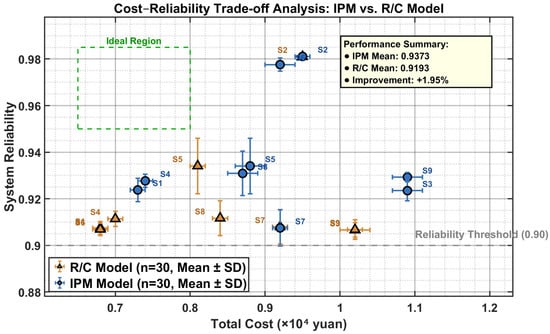
Figure 3. Cost–Reliability Trade-off Analysis for the IPM and R/C Models. Note: This scatter plot displays the relationship between total cost (X-axis, in 10⁴ yuan) and system reliability (Y-axis, dimensionless, and range 0–1) across all nine scenarios. The blue circles represent the IPM model results and the orange triangles represent the R/C model results. Each point shows the mean of 30 independent runs. Optimal solutions lie in the upper-left region (high reliability and low cost). The IPM generally achieved better positions closer to this ideal region.

The statistical analysis reveals distinct performance patterns. The IPM demonstrated significant superiority in Scenarios 1, 3, 4, 5, 6, 8, and 9, with reliability improvements of 1.80%, 1.87%, 1.80%, 3.31%, 7.79%, 2.10%, and 2.48%, respectively (all p < 0.0001). Scenario 8 achieved the best cost-effectiveness, with a 2.10% reliability gain at only a 3.38% cost increase. Scenario 6 showed the largest improvement (7.79%) but incurred a substantial cost penalty (34.70%). In contrast, Scenarios 2 and 7 showed no significant differences (p = 0.1644 and p = 0.5774), with Scenario 2 approaching the reliability ceiling (~0.98) and Scenario 7 showing slightly worse IPM performance under extended mission duration.

From Table 4, Scenario 2 benefits from baseline configurations without additional constraints, allowing both algorithms to search relatively freely. Other scenarios face compressed solution spaces from superimposed constraints. Scenario 1’s high reliability threshold (0.98) creates tension between the reliability and cost that challenges the R/C model. Scenario 3’s tight budget forces economical solutions, where the IPM better maintains reliability (0.9235 vs. 0.9066). Scenarios 4 and 5 reveal how limiting critical spare parts compromises system redundancy, with the IPM navigating these structural constraints more effectively through explicit dual-objective optimization. Scenario 6’s raised minimum configurations elevate baseline support but intensify cost pressure, yielding the IPM’s largest reliability gain. Scenario 7’s extended duration increases cumulative failure probability, where both models perform similarly near the achievable ceiling. Scenario 8’s increased failure rates create challenging conditions where the IPM’s balanced optimization proves most valuable. Scenario 9’s price increase disrupts the cost–reliability equilibrium, yet the IPM maintains a significant improvement.

These observations suggest framework enhancements through dynamic weight adjustment and adaptive mechanisms. For extreme reliability demands, increasing the reliability weight to 0.7–0.8 could ensure baseline performance. Under budget constraints, elevating cost weight would identify economical solutions. For parameter deterioration scenarios, adaptive mechanisms adjusting pheromone intensity based on environmental conditions could improve solution quality.

Statistical evidence demonstrates IPM superiority across scenarios, achieving a mean reliability of 0.9281 versus 0.9067 for the R/C model (2.35% improvement). The IPM meets the 90% threshold in all scenarios except Scenario 7, whereas the R/C model fails in Scenarios 1, 3, 8, and 9. Small standard deviations (typically <0.005) indicate stable, reproducible solutions essential for practical deployment. Figure 4 illustrates this consistent performance advantage with reduced variance.

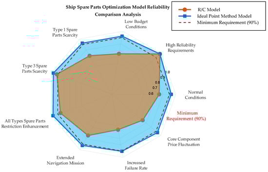
Figure 4. Reliability Comparison Radar Chart for the IPM and R/C Models Across Nine Scenarios. Note: Each radial axis represents one scenario (Scenarios 1–9), with reliability values scaled from the center (0) to the edge (1.0). The blue polygon shows IPM model performance, whereas the orange polygon shows R/C model performance. Larger polygon areas indicate higher overall reliability across scenarios. The data represent the mean values from 30 independent runs per scenario. The IPM polygon consistently extends beyond the R/C polygon, demonstrating superior reliability.

Scenario 2 reveals convergence behavior under stringent requirements (R ≥ 0.98). Both models achieved nearly identical reliability (0.9811 vs. 0.9810) with comparable costs, showing no statistical significance (p = 0.1644). When requirements approach the physical ceiling, the choice of objective function has a diminishing impact as the constrained solution space narrows substantially. Although the IPM shows no clear advantage at these boundaries, it maintains competitive performance without penalties.

The IPM exhibits superior robustness in challenging scenarios. Under increased failure rates (Scenario 8), the IPM maintains 0.9309 ± 0.0095 reliability, versus 0.9117 ± 0.0075 for the R/C model (p < 0.0001), achieving excellent cost-effectiveness with a 2.10% reliability gain for a 3.38% cost increase. Under budget pressure (Scenario 3), the IPM achieves 0.9235 ± 0.0043 reliability versus 0.9066 ± 0.0031 (p < 0.0001). Consistently small standard deviations demonstrate algorithmic stability, which is valuable for operational planning.

5.5. Parameter Sensitivity Analysis

Systematic sensitivity analyses validated the framework’s robustness using Scenario 1 as the baseline. Six parameters were tested across five values with ten runs each. Figure 5 presents a comprehensive visualization of parameter sensitivity, comparing the reliability performance of both R/C and IPM models across all tested parameters, with error bars indicating the variation range. Figure 6 further illustrates the variation percentages, highlighting the relative stability of each parameter.

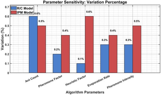
Figure 5. Parameter Sensitivity Analysis: Reliability Comparison.

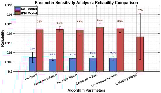
Figure 6. Parameter Sensitivity: Variation Percentage.

As illustrated in Figure 5 and Figure 6, both models demonstrate remarkable algorithmic stability under parameter perturbations. The five ACO parameters (ant count, $\alpha$, $\beta$, $\rho$, and $Q$) exhibited consistently stable performance, with reliability variations below 0.6% for both models, validating the algorithm’s robustness and suitability for practical deployment without extensive fine-tuning. The error bars in Figure 5 clearly show the minimal impact of parameter variations on system reliability. Notably, the IPM model consistently achieved higher reliability levels (0.918–0.930) compared to the R/C model (0.905–0.910) across all parameter ranges, demonstrating superior performance stability.

Figure 6 reveals that the heuristic factor $\beta$ exhibited the most stable behavior, with only 0.1–0.6% variation, whereas the ant count parameter showed slightly higher but still acceptable variations (0.5–0.6%). The pheromone-related parameters ($\alpha$, $\rho$, and $Q$) all demonstrated excellent stability, with variations below 0.5%, confirming the default configuration (40 ants, $\alpha =1.5$, $\beta =5$, $\rho =0.2$, and $Q=100$) as appropriate. The reliability weight ${\omega }^R$ exhibited the expected intentional sensitivity (2.7% variation): at ${\omega }^R$ = 0.3, the IPM emphasized economy (0.9063 reliability, cost 0.68); at ${\omega }^R$ = 0.7, it prioritized safety (0.9304 reliability, cost 0.75, 10% premium); the baseline ${\omega }^R$ = 0.5 provides balanced performance (0.9219 reliability, 0.72 cost).

The visual analysis conclusively demonstrates robust algorithm performance across all parameters except ${\omega }^R$, which intentionally controls reliability–cost trade-offs. The comparative bar charts reveal that the IPM model not only achieves consistently higher reliability but also maintains comparable stability across all parameter ranges, enabling mission-specific optimization strategies without extensive tuning.

6. Conclusions

This research effectively addresses the limitations of the traditional R/C model in ship spare parts optimization by introducing the IPM and an improved ant colony algorithm. The IPM successfully balances reliability and cost objectives, ensuring reasonable cost control while maintaining system reliability. The improved ant colony algorithm enhances optimization performance under complex constraint conditions by utilizing multi-dimensional pheromone matrices, adaptive update mechanisms, and a three-level constraint handling strategy.

Our selection of the R/C model as the primary benchmark reflects its established prevalence in maritime spare parts literature and operational practice. Although general-purpose multi-objective algorithms, such as NSGA-II and MOPSO, offer powerful optimization capabilities, they require substantial domain-specific modifications to accommodate the discrete decision variables, hierarchical three-level constraint structure, and real-time deployment requirements of ship spare parts allocation. Notably, existing studies applying NSGA-II to similar combinatorial problems typically report convergence requiring 150–300 iterations, whereas our approach achieves stable solutions at 68 iterations, with solution quality variance below 1%. The IPM framework additionally addresses a practical limitation of Pareto-based approaches by directly generating single actionable solutions under specified weight preferences, which aligns better with operational decision-making workflows.

Statistical rigor was ensured through 30 independent runs per scenario. Paired t-tests confirmed that the IPM achieved statistically significant reliability improvements in seven out of nine scenarios (p < 0.0001), with an average improvement of 2.35%. The systematic parameter sensitivity analysis demonstrated that the algorithm maintains stable performance, with variations typically under 0.6% across ant count, $\alpha$, $\beta$, $\rho$, and $Q$ parameters, validating its robustness for practical deployment. The reliability weight w₁ should be adaptively adjusted based on mission priorities to optimize the reliability–cost trade-off.

However, several limitations warrant acknowledgment. Although the Poisson distribution and two-state assumptions offer computational efficiency, they may not fully capture all failure characteristics. Sensitivity analyses indicate that for components with increasing failure rates, Weibull distributions with a shape parameter $\beta$ > 1 would yield 5–12% lower reliability estimates than the Poisson model, whereas for highly reliable components, exponential approximations may underestimate reliability by 3–6%. The current research primarily focuses on static optimization and does not account for dynamic changes in spare parts demand in evolving environments. Moreover, although experimental validation is based on simulation data, it lacks validation through real-world cases. Direct empirical comparison with contemporary multi-objective frameworks would strengthen the generalizability claims, representing a valuable direction for future investigation once these algorithms are appropriately adapted to maritime constraint architectures.

Future research should explore more flexible failure distribution models to improve accuracy across diverse component types, enhance the model’s practicality for dynamic environments, and strengthen integration with real-world engineering applications, facilitating the transition of ship spare parts optimization from theoretical research to engineering practice. The comparative verification across nine typical scenarios demonstrates the effectiveness and robustness of the proposed method, offering a solid foundation for decision-making in ship equipment support.

Appendix A.1

Algorithm A1. Three-level Constraint Handling Mechanism

function [best_solution, best_reliability, best_cost] = RC_Model_ACO() Initialize pheromone matrix; Set best_ratio to zero; while not converged do      for each ant do           Generate feasible solution satisfying:             - Minimum quantity constraints             - Total quantity constraint             - Minimum reliability requirement           end           Calculate system reliability R using Poisson distribution;           Calculate total cost C from unit costs;           Compute R/C ratio as fitness value;           if R/C ratio > best_ratio then             Update best solution;             Update best_ratio;             Record reliability and cost;           end      end      Calculate pheromone increment for each solution;      Update pheromone matrix based on solution quality;      Apply pheromone evaporation; end return best_solution, best_reliability, best_cost; end

Appendix A.2

Algorithm A2. Improved Ant Colony Algorithm for Spare Parts Optimization

function [best_solution, best_reliability, best_cost] = Ideal_Point_Method_ACO() Determine ideal point (maximum reliability, minimum cost); Calculate normalization bounds for objectives; Initialize pheromone matrix; Set best_distance to infinity; while not converged do      for each ant do           Generate feasible solution satisfying:             - Minimum quantity constraints             - Total quantity constraint             - Minimum reliability requirement           end           Calculate system reliability R using Poisson distribution;           Calculate total cost C from unit costs;           Normalize reliability to [0, 1] range;           Normalize cost to [0, 1] range;           Calculate weighted Euclidean distance to ideal point:             distance = sqrt(w1 × (R_normalized - R_ideal)2 +                          w2 × (C_normalized - C_ideal)2);           end           if distance < best_distance then             Update best solution;             Update best_distance;             Record reliability and cost;           end      end      Calculate pheromone increment inversely proportional to distance;      Update pheromone matrix based on solution quality;      Apply pheromone evaporation; end return best_solution, best_reliability, best_cost; end

References

- Xiao, B.; Liu, C.; Jiang, T.J. Multi objective optimization of ship spare parts maintenance based on Improved Genetic Algorithm. E3S Web Conf. 2021, 253, 02016. [Google Scholar] [CrossRef]
- Wang, H.; Liu, H.; Shao, S.; Zhang, Z. Methodology of shipboard spare parts requirements based on whole part repair strategy. Mathematics 2024, 12, 3053. [Google Scholar] [CrossRef]
- Zhang, J.R. Research on spare parts optimization method for complex electronic equipment based on monte carlo simulation. Consum. Electron. 2024, 9, 6–12. [Google Scholar]
- Dong, Z.Q.; Tang, S.K.; Li, C.Y.; Nie, L.; Zhou, X.D.; Ding, S.T.; Fan, Y.Y. Configuration method of naval gun equipment spare parts based on multi-agent simulation. Chin. J. Ship Res. 2022, 17, 228–234. [Google Scholar]
- Li, W.; Li, H.J.; Li, H. Optimization of spare parts configuration scheme for ship equipment based on multi-agent simulation. Proc. SPIE 2024, 13445, 134452L. [Google Scholar]
- Fu, L.Y.; Liu, C.Y.; Dong, Q.; Tang, L.; Weng, X.H.; Xian, K. Research on multi-objective configuration optimization of ship spare with exponential distribution demand. In Proceedings of the 2018 2nd International Conference on Management Engineering, Software Engineering and Service Sciences (ICMSS 2018), Wuhan, China, 13–15 January 2018. [Google Scholar]
- Li, Y.H.; Zhang, Y.; Yong, Q.; Chen, Z.M. Research on optimization method of ship spare parts allocation based on improved discrete crow search algorithm. Commun. Comput. Inf. Sci. 2024, 2139, 211–221. [Google Scholar]
- Liu, G.; Zhong, X.J.; Dong, P. Research on optimization model of ship electronic equipment spare parts based on genetic algorithm and neural network. Ship Sci. Technol. 2008, 30, 138–142. [Google Scholar]
- Jiang, W.; Sheng, W.; Yang, L.; Fan, Y.L. Optimization configuration of phased array radar spare parts under condition-based maintenance. Syst. Eng. Electron. 2017, 39, 2052–2057. [Google Scholar]
- Mei, D.; Wang, G.B.; Ye, Z.H.; Shen, J.; Feng, H. Optimization configuration of spare parts for motor control and power distribution systems. Electr. Mach. Control Appl. 2018, 45, 41–45, 63. [Google Scholar]
- Gong, L.X.; Fan, Y.M.; Liang, J.L.; Xiao, M.L.; Lei, B.W. Cost and availability-oriented ship redundant system and spare parts inventory optimization model. J. Nav. Univ. Eng. 2025, 37, 1–8. [Google Scholar]
- Tang, Z.; Lin, M.C.; Wang, C.Y. Critical Evaluation and Optimal Allocation Model of Ship Spare Parts. In Proceedings of the 4th International Conference on Modelling, Simulation and Applied Mathematics (MSAM 2020), Wuhan, China, 12–13 January 2020. [Google Scholar]
- Zhou, L.; Meng, J.; Li, Y.; Li, W. Optimization method for radiation interference cancellation equipment of ship spare parts configuration with criticality under multiple constraints. Syst. Eng. Electron. 2020, 42, 365–373. [Google Scholar]
- Dong, Z.Q.; Tang, S.K.; Zhou, X.D.; Nie, L.; Fan, Y.Y. Optimization configuration method of ship accompanying spare parts based on tabu search. Ship Eng. 2023, 45, 138–143. [Google Scholar]
- Zhang, R.; Liu, C.L.; Shao, H.W.; Zhou, H.F.; Zhang, J. Multi-constraint ship spare parts configuration optimization based on improved particle swarm algorithm. Ship Electron. Eng. 2023, 43, 102–108. [Google Scholar]
- Li, Z.Q.; Xu, T.X.; Dong, Q.; Zeng, X.; Liu, Y.D. Optimization configuration method for ship-borne spare parts based on PDF-CDF. Fire Control Command. Control. 2018, 43, 17–21. [Google Scholar]
- Zhai, Y.L.; Qi, R.; Shao, S.S. Ship spare parts utilization rate calculation and application under periodic supply conditions. Comput. Simul. 2025, 42, 16–21. [Google Scholar]
- Ruan, M.Z.; Qian, C.; Wang, R.; Wang, J.L. Ship formation spare parts configuration optimization under regular support mode. Syst. Eng. Theory Pract. 2018, 38, 2441–2448. [Google Scholar]
- Chai, Z.J.; Wang, Z.B. Application of improved particle swarm algorithm in ship spare parts configuration optimization problem. Comput. Digit. Eng. 2021, 49, 493–495+588. [Google Scholar]
- Li, Q.J. Ship electronic equipment spare parts optimization model based on ant colony algorithm and extreme learning machine. Ship Sci. Technol. 2022, 44, 158–161. [Google Scholar]
- Sha, J.; Leng, J.; Mao, H.; Pei, J.; Diao, K. Research Progress in Predictive Maintenance of Offshore Platform Structures Based on Digital Twin Technology. J. Mar. Sci. Appl. 2025, 24, 877–899. [Google Scholar] [CrossRef]
- Lv, Z.; Lv, H.; Fridenfalk, M. Digital Twins in the Marine Industry. Electronics 2023, 12, 2025. [Google Scholar] [CrossRef]
- Kalafatelis, A.S.; Nomikos, N.; Giannopoulos, A.; Alexandridis, G.; Karditsa, A.; Trakadas, P. Towards Predictive Maintenance in the Maritime Industry: A Component-Based Overview. J. Mar. Sci. Eng. 2025, 13, 425. [Google Scholar] [CrossRef]
- Budimir, D.; Medić, D.; Ružić, V.; Kulej, M. Integrated Approach to Marine Engine Maintenance Optimization: Weibull Analysis, Markov Chains, and DEA Model. J. Mar. Sci. Eng. 2025, 13, 798. [Google Scholar] [CrossRef]
- Karkaria, V.; Tsai, Y.; Chen, Y.; Chen, W. An optimization-centric review on integrating artificial intelligence and digital twin technologies in manufacturing. Eng. Optim. 2025, 57, 161–207. [Google Scholar] [CrossRef]
- Liu, H.; Cheng, K.; Gao, S. Research on ship spare parts optimization model based on cost-effectiveness analysis. Electron. Des. Eng. 2016, 24, 1–4. [Google Scholar]
Disclaimer/Publisher’s Note: The statements, opinions and data contained in all publications are solely those of the individual author(s) and contributor(s) and not of MDPI and/or the editor(s). MDPI and/or the editor(s) disclaim responsibility for any injury to people or property resulting from any ideas, methods, instructions or products referred to in the content. |
© 2025 by the authors. Licensee MDPI, Basel, Switzerland. This article is an open access article distributed under the terms and conditions of the Creative Commons Attribution (CC BY) license (https://creativecommons.org/licenses/by/4.0/).