Adaptive Optimization for Stochastic Renewal Systems

Abstract

This paper considers online optimization for a sequence of tasks. Each task can be processed in one of multiple processing modes that affect the duration of the task, the reward earned, and an additional vector of penalties (such as energy or cost). Let $A\left[k\right]$ be a random matrix that specifies the parameters of task k. The goal is to observe $A\left[k\right]$ at the start of task k and then choose a processing mode for the task so that, over time, time average reward is maximized subject to time average penalty constraints. This is a renewal optimization problem. It is challenging because the probability distribution for the $A\left[k\right]$ sequence is unknown. Efficient decisions must be learned in a timely manner. Prior work shows that any algorithm that comes within $ϵ$ of optimality must have $\Omega (1/{ϵ}^2)$ convergence time. The only known algorithm that can meet this bound operates without time average penalty constraints and uses a diminishing stepsize that cannot adapt when probabilities change. This paper develops a new algorithm that is adaptive and comes within $\Theta \left(ϵ\right)$ of optimality for any interval of $\Theta (1/{ϵ}^2)$ tasks over which probabilities are held fixed.

1. Introduction

This paper considers online optimization for a system that performs a sequence of tasks. At the start of task $k\in \{1,2,3,\dots \}$, a matrix $A\left[k\right]$ of parameters about the task is revealed. The controller observes $A\left[k\right]$ and then makes a decision about how the task should be processed. The decision, together with $A\left[k\right]$, determines the duration of the task, the reward earned by processing that task, and a vector of additional penalties. Specifically, define

$$\begin{array}{cc}\hfill T\left[k\right]& = \mathrm{duration} \mathrm{of} \mathrm{task} k\hfill \\ \hfill R\left[k\right]& = \mathrm{reward} \mathrm{of} \mathrm{task} k\hfill \\ \hfill Y\left[k\right]& = (Y_1\left[k\right],\dots ,Y_n\left[k\right])\hfill \\ \hfill & = \mathrm{penalty} \mathrm{vector} \mathrm{for} \mathrm{task} k\hfill \end{array}$$

where n is a fixed positive integer. The goal is to make decisions over time that maximize the time average reward subject to a collection of time average penalty constraints. This problem has a number of applications, including image classification, video processing, wireless multiple access, and transportation scheduling.

For example, consider a computational device that performs back-to-back image classification tasks with the goal of maximizing time average profit subject to a time average power constraint of $p_{av}$ and an average per-task quality constraint of $q_{av}$. For each task, the device chooses from a collection of classification algorithms, each having a different duration of time and yielding certain profit, energy, and quality characteristics. The number of options for task k is equal to the number of rows of matrix $A\left[k\right]$. Numerical values for each option are specified in the corresponding row. Suppose the controller observes the following matrix $A\left[1\right]$ for task 1:

$$A\left[1\right]=\begin{array}{ccccc}\mathrm{duration}& \mathrm{profit}& \mathrm{energy}& \mathrm{quality}& \\ 5.1& 3.6& 2.3& 0.5& \mathrm{alg}1\\ 7.0& 2.8& 1.5& 1.0& \mathrm{alg}2\\ 10.2& 3.0& 1.1& 1.0& \mathrm{alg}3\end{array}$$

(1)

Choosing a classification algorithm for task 1 reduces to choosing one of the three rows of $A\left[1\right]$. Suppose we choose row 2 (algorithm 2). Then, task 1 will have a duration of $7.0$ units of time, as illustrated by the width $T\left[1\right]$ in the timeline of Figure 1. Also, the task will have profit, energy, and quality of $2.8$, $1.5$, and $1.0$. If we had instead chosen row 1, then the task duration would be lower and profit would be higher, but the energy consumption would be higher and the task would have lower quality. It is not obvious what decision helps to maximize the time average profit subject to the power and quality constraints. Moreover, the matrices for future tasks can have different row sizes, each matrix $A\left[k\right]$ is only revealed at the start of task k, and the probability distribution for $A\left[k\right]$ is unknown.

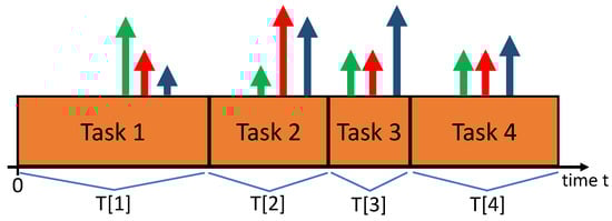
Figure 1. Four sequential tasks in the timeline. Vertical arrows for each task k represent values for reward $R\left[k\right]$ and penalty vector $Y\left[k\right]$. In this example, green is reward (profit), red is energy, blue is quality. Vector $\left(T\right[k],R[k],Y[k\left]\right)$ depends on choices made at the start of task k.

The specific constrained optimization problem for this example is

$$\begin{array}{cc}\hfill \mathrm{Maximize}:& \underset{m\to \infty }{lim}{\displaystyle \frac{{\sum }_{k=1}^{m}R\left[k\right]}{{\sum }_{k=1}^{m}T\left[k\right]}}\hfill \end{array}$$

(2)

$$\begin{array}{cc}\hfill \mathrm{Subject} \mathrm{to}:& \underset{m\to \infty }{lim}{\displaystyle \frac{{\sum }_{k=1}^{m}Energy\left[k\right]}{{\sum }_{k=1}^{m}T\left[k\right]}}\le p_{av}\hfill \end{array}$$

(3)

$$\begin{array}{cc}\hfill & \underset{m\to \infty }{lim}{\displaystyle \frac{1}{m}}{\sum }_{k=1}^{m}Quality\left[k\right]\ge q_{av}\hfill \end{array}$$

(4)

where objective (2) represents the time average profit; (3) imposes the time average power constraint; (4) imposes the per-task average quality constraint. For simplicity of this example, we assume the limits exist. This problem is more concisely posed as maximizing $\overline{R}/\overline{T}$ subject to $\overline{Energy}/\overline{T}\le p_{av}$ and $\overline{Quality}\ge q_{av}$, where $\overline{R}$, $\overline{T}$, $\overline{Energy}$, $\overline{Quality}$ are per-task averages.

Problem (2)–(4) involves ratios of averages. This paper converts such problems into a canonical form of maximizing a ratio $\overline{R}/\overline{T}$ subject to penalty constraints ${\overline{Y}}_i\le 0$ for $i\in \{1,\dots ,n\}$, where n is the number of constraints ($n=2$ in example problem (2)–(4)). The constraint $\overline{Energy}/\overline{T}\le p_{av}$ is converted to ${\overline{Y}}_1\le 0$ by defining a penalty process $Y_1\left[k\right]=Energy\left[k\right]-p_{av}T\left[k\right]$ for $k\in \{1,2,3,\dots \}$. However, adaptive minimization of the ratio $\overline{R}/\overline{T}$ is nontrivial, and new techniques are required.

Optimality for problem (2)–(4) depends on the joint probability distribution for the size and entries of matrix $A\left[k\right]$. We first assume ${\left\{A\left[k\right]\right\}}_{k=1}^{\infty }$ are independent and identically distributed (i.i.d.) as matrices over tasks $k\in \{1,2,3,\dots \}$. This yields a well-defined ergodic optimality for problem (2)–(4). However, the multi-dimensional distribution for the entries of $A\left[k\right]$ is unknown, and the parameter space is enormous. Instead of attempting to learn the distribution, this paper uses techniques similar to the drift-plus-penalty method of [1] that acts on weighted functions of the observed random $A\left[k\right]$. Specifically, this paper develops a new optimization strategy that acts on a single timescale for real-time optimization of ratios of averages.

Given $ϵ>0$, how long does it take to come within $ϵ$ of the infinite horizon optimality for problem (2)–(4)? This question is partially addressed in the prior work [2] for problems without time average penalty constraints. That prior work uses a Robbins–Monro algorithm with a vanishing stepsize. It cannot adapt if probability distributions change over time. The current paper develops a new algorithm that is adaptive. While infinite horizon optimality is defined by imagining $\left\{A\right[k\left]\right\}$ as an infinite i.i.d. sequence, our algorithm can be analyzed over any finite block of m tasks $\{k_0,k_0+1,\dots ,k_0+m-1\}$ for which i.i.d. behavior is assumed. Indeed, fix any algorithm parameter $ϵ>0$ and consider any integer $m\ge 1/{ϵ}^2$. Over any block of m tasks during which $A\left[k\right]$ is i.i.d., the time average expected performance of our algorithm is within $O\left(ϵ\right)$ of infinite horizon optimality (as defined by the $A\left[k\right]$ distribution for this block), regardless of the distribution or sample path behavior of $A\left[k\right]$ before the block. When the algorithm is implemented over all time, it tracks the new optimality that results if probability distributions change multiple times in the timeline, without knowing when changes occur, provided that each new distribution lasts for a duration of at least $\Theta (1/{ϵ}^2)$ tasks. This new $\Theta (1/{ϵ}^2)$ achievability result matches a converse bound proven for unconstrained problems in [2].

1.1. Model

Fix n as a positive integer. At the start of each task $k\in \{1,2,3,\dots \}$ the controller observes matrix $A\left[k\right]$ with size $M\left[k\right]\times (n+2)$, where $M\left[k\right]$ is the random number of processing options for task k. Each row $r\in \{1,\dots ,M[k\left]\right\}$ has the form

$$[T_r\left[k\right],R_r\left[k\right],Y_{r,1}\left[k\right],\dots ,Y_{r,n}\left[k\right]]$$

It is assumed that all rows have $T_r\left[k\right]\ge t_{min}$, where $t_{min}>0$ is some minimum task duration. Let $\left(T\right[k],R[k],Y[k\left]\right)$ be the vector of values for the row selected on task k, where $Y\left[k\right]=(Y_1\left[k\right],\dots ,Y_n\left[k\right])$. For each positive integer m, define $\overline{R}\left[m\right]$ by

$$\overline{R}\left[m\right]={\displaystyle \frac{1}{m}}{\sum }_{k=1}^{m}R\left[k\right]$$

Define $\overline{T}\left[m\right]$ and $\overline{Y}\left[m\right]$ similarly. The infinite horizon problem is

$$\begin{array}{cc}\hfill \mathrm{Maximize}:& \underset{m\to \infty }{lim\; inf}{\displaystyle \frac{\mathbb{E}\left[\overline{R}\left[m\right]\right]}{\mathbb{E}\left[\overline{T}\left[m\right]\right]}}\hfill \end{array}$$

(5)

$$\begin{array}{cc}\hfill \mathrm{Subject} \mathrm{to}:& \underset{m\to \infty }{lim\; sup}\mathbb{E}\left[{\overline{Y}}_i\left[m\right]\right]\le 0\forall i\in \{1,\dots ,n\}\hfill \end{array}$$

(6)

$$\begin{array}{cc}\hfill & \left(T\right[k],R[k],Y[k\left]\right)\in Row\left(A\right[k\left]\right)\forall k\in \{1,2,3,\dots \}\hfill \end{array}$$

(7)

where $Row\left(A\right[k\left]\right)$ denotes the set of rows of matrix $A\left[k\right]$. Note that $T\left[k\right]\ge t_{min}>0$ always, so there is no divide-by-zero issue.

Problem (5)–(7) is assumed to be feasible, meaning it is possible to satisfy the constraints (6) and (7). Let ${\theta }^{*}$ denote the optimal objective in (5). The formulation (5)–(7) has two differences in comparison with the introductory example (2)–(4): (i) all time average constraints are expressed as a single average (rather than a ratio); (ii) sample path limits are replaced by limits that use expectations. This is similar to the treatment in [2]. This preserves the infinite horizon value of ${\theta }^{*}$ and facilitates analysis of adaptation time.A decision policy is said to be an $ϵ$-approximation with convergence time d if

$$\begin{array}{cc}\hfill & {\displaystyle \frac{\mathbb{E}\left[\overline{R}\left[m\right]\right]}{\mathbb{E}\left[\overline{T}\left[m\right]\right]}}\le {\theta }^{*}+ϵ\forall m\ge d\hfill \end{array}$$

(8)

$$\begin{array}{cc}\hfill & \mathbb{E}\left[{\overline{Y}}_i\left[m\right]\right]\le ϵ\forall i\in \{1,\dots ,n\}\forall m\ge d\hfill \end{array}$$

(9)

A decision policy is said to be an $O\left(ϵ\right)$-approximation (with convergence time d) if all appearances of $ϵ$ in the above definition are replaced by some constant multiple of $ϵ$.

1.2. Prior Work

The fractional structure of the objective (5) is similar in spirit to a linear fractional program. Linear fractional programs can be converted to linear programs using a nonlinear change in variables (see [3,4]). This conversion is used in [3] for offline design of policies for embedded Markov decision problems. Such methods cannot be directly used for our online problem because time averages are not preserved under nonlinear transformations. Related nonlinear transformations are used in [5] for offline control for opportunistic Markov decision problems where states include an $A\left[k\right]$ process similar to the current paper. The work in [5] discusses how offline strategies can be leveraged for online use (such as with a two-timescale approach), although overall convergence time is unclear.

The problem (5)–(7) is posed in [6], where it is called a renewal optimization problem (see also Chapter 7 of [1]). The solution in [6] constructs virtual queues for each time average inequality constraint (6) and makes a decision for each task k to minimize a drift-plus-penalty ratio:

$${\displaystyle \frac{\mathbb{E}\left[\Delta \left[k\right]-vR\left[k\right]\left|H\right[k]\right]}{\mathbb{E}\left[T\left[k\right]\left|H\right[k]\right]}}$$

(10)

where $\Delta \left[k\right]$ is the change in a Lyapunov function on the virtual queues; v is a parameter that affects accuracy; $H\left[k\right]$ is system history before task k. Exact minimization of (10) is impossible unless the distribution for $A\left[k\right]$ is known. A method for approximately minimizing (10) by sampling $A\left[k\right]$ over a window of previous tasks is developed in [6], although only a partial convergence analysis is given there. This prior work is based on the Lyapunov drift and max-weight scheduling methods developed for fixed timeslot queuing systems in [7,8]. Data center applications of renewal optimization are in [9]. Asynchronous renewal systems are treated in [10].

A different approach in [2] is used for a problem that seeks only to maximize time average reward $\overline{R}/\overline{T}$ (with no penalties $Y\left[k\right]$). For each task k, that method chooses $\left(T\right[k],R[k\left]\right)\in Row\left(A\right[k\left]\right)$ to maximize $R\left[k\right]-\theta [k-1]T\left[k\right]$, where $\theta [k-1]$ is an estimate of ${\theta }^{*}$ that is updated according to a Robbins–Monro iteration:

$$\theta \left[k\right]=\theta [k-1]+\eta \left[k\right]\left(R\right[k]-\theta [k-1\left]T\right[k\left]\right)$$

(11)

where $\eta \left[k\right]$ is a stepsize. See [11] for the original Robbins–Monro algorithm and [12,13,14,15,16,17] for extensions in other contexts. The approach (11) is desirable because it does not require sampling from a window of past $A\left[k\right]$ values. Further, under a vanishing stepsize rule, the optimality gap decreases like $O(1/\sqrt{k})$, which is asymptotically optimal [2]. However, it is unclear how to extend this method to handle time average penalties $Y\left[k\right]$. Further, while the vanishing stepsize enables fast convergence, it makes increasing investments in the probability model and cannot adapt if probabilities change. The work in [2] shows a fixed stepsize rule is better for adaptation but has a slower convergence time of $O(1/{ϵ}^3)$.

Fixed stepsizes are known to enable adaptation in other contexts. For online convex optimization, it is shown in [18] that a fixed stepsize enables the time-averaged cost to be within $O\left(ϵ\right)$ of optimality (as compared with the best fixed decision in hindsight) over any sequence of $\Theta (1/{ϵ}^2)$ steps. For adaptive estimation, work in [19] considers the problem of removing bias from Markov-based samples. The work in [19] develops an adaptive Robbins–Monro technique that averages between two fixed stepsizes. Adaptive algorithms are also of interest in convex bandit problems, see [20,21].

A different type of problem is nonlinear robust optimization that seeks to solve a deterministic nonlinear program involving a decision vector x and a vector of (unchosen) uncertain values u (see [22]). The robust design treats worst-case behavior with constraints such as $c(x,u)\le 0$ for all $u\in \mathcal{U}\left(x\right)$, where $\mathcal{U}\left(x\right)$ is a (possibly infinite) set of possible values of u given the decision vector x. Iterative methods, such as those in [23], use gradients and linear approximations to sequentially calculate updates that get closer to minimizing a cost function subject to the robust constraint specifications.

Our problem is an opportunistic scheduling problem because $A\left[k\right]$ is revealed at the start of each task k (before a scheduling decision is made). While $A\left[k\right]$ can be viewed as helpful side information, it is challenging to make optimal use of this side information. The policy space huge: Optimality depends on the full (and unknown) joint distribution of entries in matrix $A\left[k\right]$. A different class of problems, called vector-based bandit problems, has a simpler policy space where there is no $A\left[k\right]$ information. There, the controller pulls an arm from a fixed set of m arms, each arm giving a vector-based reward with an unknown distribution that is the same each time it is pulled. In that context, optimality depends only on the mean rewards. Estimation of the means can be performed efficiently by exploring each arm according to various bandit techniques such as the resource-constrained techniques in [24,25,26]. Such problems have a different learning structure that does not relate to the current paper.

1.3. Our Contributions

We develop an algorithm for renewal optimization that does not require probability information or sampling from the past. The algorithm has explicit convergence guarantees and meets the optimal asymptotic convergence time bound of [2]. Unlike the Robbins–Monro method in [2], our new algorithm allows for penalty constraints. Furthermore, our algorithm is adaptive and achieves performance within $O\left(ϵ\right)$ of optimality over any sequence of $\Theta (1/{ϵ}^2)$ tasks. This fast adaptation is enabled by a new hierarchical decision structure.

2. Preliminaries

2.1. Notation

For $x,y\in {\mathbb{R}}^n$ we use $x^{\top }y={\sum }_{i=1}^n{x}_i{y}_i$ and $\left|\right|x\left|\right|=\sqrt{{\sum }_{i=1}^n{x}_i^2}$. In this paper, we use the following vectors and constants:

• $A\left[k\right]=$ matrix for task k (for row selection)
• $T\left[k\right]=$ duration of task k
• $R\left[k\right]=$ reward of task k
• $Y\left[k\right]=(Y_1\left[k\right],\dots ,Y_n\left[k\right])=$ vector of penalties for task k
• $Q\left[k\right]=(Q_1\left[k\right],\dots ,Q_n\left[k\right])=$ vector of virtual queues for penalty constraints
• $J\left[k\right]=$ virtual queue used to optimize reward
• $v=$ weight emphasis on reward
• $q_i=$ size upper bound parameter for virtual queue $Q_i\left[k\right]$
• ${\theta }^{*}=$ optimal time average reward
• $r_{max}=$ upper bound on $R\left[k\right]$
• $c=$ upper bound on $\left|\right|Y\left[k\right]\left|\right|$
• $y_{i,min},y_{i,max}=$ bounds on $Y_i\left[k\right]$ ($-y_{i,min}\le Y_i\left[k\right]\le y_{i,max}$)
• $[t_{min},t_{max}]=$ bounds on $T\left[k\right]$
• ${\gamma }_{min}=1/t_{max}$, ${\gamma }_{max}=1/t_{min}$
• $s=$ Slater condition parameter
• $b,{\beta }_1,{\beta }_2,d_0,d_1,d_2=$ constants in theorems (based on $q_i,r_{max},c,t_{min},t_{max},y_{i,min},y_{i,max}$).

2.2. Boundedness Assumptions

Assume the following bounds hold for all $k\in \{1,2,3,\dots \}$, all $A\left[k\right]$, and all choices of $\left(T\right[k],R[k],Y[k\left]\right)\in Row\left(A\right[k\left]\right)$:

$$\begin{array}{cc}\hfill & t_{min}\le T\left[k\right]\le t_{max}\hfill \end{array}$$

(12)

$$\begin{array}{cc}\hfill & 0\le R\left[k\right]\le r_{max}\hfill \end{array}$$

(13)

$$\begin{array}{cc}\hfill & \left|\right|Y\left[k\right]\left|\right|\le c\hfill \end{array}$$

(14)

$$\begin{array}{cc}\hfill & -y_{i,min}\le Y_i\left[k\right]\le y_{i,max}\forall i\in \{1,\dots ,n\}\hfill \end{array}$$

(15)

where $t_{min}$, $t_{max}$, $r_{max}$, c, $y_{i,min}$, $y_{i,max}$ are nonnegative constants (with $t_{min}>0$). Constraint (13) assumes all rewards $R\left[k\right]$ are nonnegative. This is without loss of generality: If the system can have negative rewards in some bounded interval $-r_{min}\le R\left[k\right]\le r_{max}$, where $r_{min}>0$, we define a new nonnegative reward $G\left[k\right]=R\left[k\right]+(r_{min}/t_{min})T\left[k\right]$. The objective of maximizing $\overline{G}/\overline{T}$ is the same as the objective of maximizing $\overline{R}/\overline{T}$.

2.3. The Sets $\Gamma$ and $\overline{\Gamma }$

Assume ${\left\{A\left[k\right]\right\}}_{k=1}^{\infty }$ is a sequence of i.i.d. random matrices with an unknown distribution. (When appropriate, this is relaxed to assume i.i.d. behavior occurs only over a finite block of consecutive tasks.) For $k\in \{1,2,3,\dots \}$, define a decision vector $\left(T\right[k],R[k],Y[k\left]\right)$ as a random vector that satisfies

$$\left(T\right[k],R[k],Y[k\left]\right)\in Row\left(A\right[k\left]\right)$$

Let $\Gamma \subseteq {\mathbb{R}}^{n+2}$ be the set of all expectations $\mathbb{E}\left[\left(T\right[k],R[k],Y[k\left]\right)\right]$ for a given task k, considering all possible decision vectors. The set $\Gamma$ depends on the (unknown) distribution of $A\left[k\right]$ and considers all conditional probabilities for choosing a row given the observed $A\left[k\right]$. The ${\left\{A\left[k\right]\right\}}_{k=1}^{\infty }$ matrices are i.i.d. and so $\Gamma$ is the same for all $k\in \{1,2,3,\dots \}$. It can be shown that $\Gamma$ is nonempty, bounded, and convex (see Section 4.11 in [1]). Its closure $\overline{\Gamma }$ is compact and convex. Define the history up to task m as

$$H\left[m\right]=\left(A\right[1],A[2],\dots ,A[m-1\left]\right)$$

where $H\left[1\right]$ is defined to be the constant 0.

Lemma 1.

Suppose ${\left\{A\left[k\right]\right\}}_{k=1}^{\infty }$ are i.i.d. and satisfy the boundedness assumptions (12)–(15). Then, for every $(t,r,y)\in \Gamma$ and $k\in \{1,2,3,\dots \}$, there exists a random decision vector

$$(T^{*}\left[k\right],R^{*}\left[k\right],Y^{*}\left[k\right])\in Row\left(A\left[k\right]\right)$$

that is independent of $H\left[k\right]$ and that satisfies (with probability 1):

$$\mathbb{E}\left[(T^{*}\left[k\right],R^{*}\left[k\right],Y^{*}\left[k\right])|H\left[k\right]\right]=(t,r,y)$$

Proof. 

By definition of $\Gamma$, given any $(t,r,y)\in \Gamma$, there is a conditional distribution for choosing a row of $A\left[k\right]$ (given the observed $A\left[k\right]$) under which the (unconditional) expected value of the chosen row is $(t,r,y)$. Let $U\left[k\right]\sim Unif[0,1]$ be a random variable that is independent of $\left(A\right[k],H[k\left]\right)$. Use $U\left[k\right]$ to implement the randomized row selection (according to the desired conditional distribution) after $A\left[k\right]$ is observed. Formally, the random row $(T^{*}\left[k\right],R^{*}\left[k\right],Y^{*}\left[k\right])$ can be viewed as a Borel measurable function of $\left(A\right[k],U[k\left]\right)$. (See Proposition 5.13 in [27], where $\xi$ there plays the role of our $(T^{*}\left[k\right],R^{*}\left[k\right],Y^{*}\left[k\right])$ which takes values in the Borel space ${\mathbb{R}}^{n+2}$; $\eta$ plays the role of our $A\left[k\right]$; $\zeta$ plays the role of our $H\left[k\right]$; $\nu$ plays the role of our $U\left[k\right]$). Since $\left(A\right[k],U[k\left]\right)$ is independent of history $H\left[k\right]$, the resulting random row $(T^{*}\left[k\right],R^{*}\left[k\right],Y^{*}\left[k\right])$ is independent of $H\left[k\right]$ (so with probability 1, its conditional expectation given $H\left[k\right]$ is the same as its unconditional expectation). □

2.4. The Deterministic Problem

For analysis of our stochastic problem, it is useful to consider the closely related deterministic problem

$$\begin{array}{cc}\hfill \mathrm{Maximize}:& r/t\hfill \end{array}$$

(16)

$$\begin{array}{cc}\hfill \mathrm{Subject} \mathrm{to}:& y_i\le 0\forall i\in \{1,\dots ,n\}\hfill \end{array}$$

(17)

$$\begin{array}{cc}\hfill & (t,r,y)\in \overline{\Gamma }\hfill \end{array}$$

(18)

where $\overline{\Gamma }$ is the closure of $\Gamma$. All points $(t,r,y)\in \overline{\Gamma }$ have $t\ge t_{min}>0$, so there are no divide-by-zero issues. Using arguments similar to those in Section 4.11 in [1], it can be shown that (i) the stochastic problem (5)–(7) is feasible if and only if the deterministic problem (16)–(18) is feasible; (ii) if feasible, the optimal objective values are the same. Specifically, if $(t^{*},r^{*},y^{*})$ solves (16)–(18), then

$${\theta }^{*}=r^{*}/t^{*}$$

where ${\theta }^{*}$ is the optimal objective for both the deterministic problem (16)–(18) and the stochastic problem (5)–(7). The deterministic problem (16)–(18) seeks to maximize a continuous function $r/t$ over the compact set defined by constraints (17) and (18), so it has an optimal solution whenever it is feasible.

When $n>0$ (so there is at least one time average penalty constraint of the form (17)), we assume a Slater condition that is more stringent than mere feasibility: There is a value $s>0$ and a vector $(t^s,r^s,y^s)\in \overline{\Gamma }$ such that

$$y_i^s\le -s\forall i\in \{1,\dots ,n\}$$

(19)

3. Algorithm Development

3.1. Parameters and Constants

The algorithm uses parameters $v>0$, $\alpha >0$, $q=(q_1,\dots ,q_n)$ with $q_i\ge 0$ for all $i\in \{1,\dots ,n\}$, to be precisely determined later. The constants $t_{min},t_{max},r_{max},y_{i,min},y_{i,max},c$ from the boundedness assumptions (12)–(15) are assumed known. Define

$${\gamma }_{min}=1/t_{max},{\gamma }_{max}=1/t_{min}$$

(20)

The algorithm introduces auxiliary variables $\gamma \left[k\right]$ chosen in the interval $[{\gamma }_{min},{\gamma }_{max}]$ for each task $k\in \{1,2,3,\dots \}$.

3.2. Intuition

For intuition, temporarily assume the following limits exist:

$$\begin{array}{cc}\hfill {\overline{Y}}_i& =\underset{m\to \infty }{lim}{\displaystyle \frac{1}{m}}{\sum }_{k=1}^m{Y}_i\left[k\right]\hfill \\ \hfill \overline{1/\gamma }& =\underset{m\to \infty }{lim}{\displaystyle \frac{1}{m}}{\sum }_{k=1}^{m}1/\gamma \left[k\right]\hfill \end{array}$$

The idea is to make decisions for row selection (and $\gamma \left[k\right]$ selection) for each task k so that, over time, the following time-averaged problem is solved:

$$\begin{array}{cc}\hfill \mathrm{Maximize}:& \underset{m\to \infty }{lim}{\displaystyle \frac{\frac{1}{m}{\sum }_{k=1}^{m}R\left[k\right]\gamma \left[k\right]/\gamma [k-1]}{\frac{1}{m}{\sum }_{k=1}^{m}1/\gamma [k-1]}}\hfill \end{array}$$

(21)

$$\begin{array}{cc}\hfill \mathrm{Subject} \mathrm{to}:& {\overline{Y}}_i\le 0\forall i\in \{1,\dots ,n\}\hfill \end{array}$$

(22)

$$\begin{array}{cc}\hfill & \overline{T}\le \overline{1/\gamma }\hfill \end{array}$$

(23)

$$\begin{array}{cc}\hfill & \gamma \left[k\right]\in [{\gamma }_{min},{\gamma }_{max}]\forall k\hfill \end{array}$$

(24)

$$\begin{array}{cc}\hfill & \left(T\right[k],R[k],Y[k\left]\right)\in Row\left(A\right[k\left]\right)\forall k\hfill \end{array}$$

(25)

$$\begin{array}{cc}\hfill & \gamma \left[k\right]\mathrm{varies} “\mathrm{slowly}” \mathrm{over} k\hfill \end{array}$$

(26)

This is an informal description because the constraint “$\gamma \left[k\right]$ varies slowly” is not precise. Intuitively, if $\gamma \left[k\right]$ does not change much from one task to the next, the above objective is close to $\overline{R}/\overline{1/\gamma }$, which (by the second constraint) is less than or equal to the desired objective $\overline{R}/\overline{T}$. This is useful because, as we show, the above problem can be treated using a novel hierarchical optimization method.

3.3. Virtual Queues

To enforce the constraints ${\overline{Y}}_i\le 0$, for each $i\in \{1,\dots ,n\}$ define a process $Q_i\left[k\right]$ with initial condition $Q_i\left[1\right]=0$ and update equation

$$Q_i[k+1]={[Q_i\left[k\right]+Y_i\left[k\right]]}_0^{q_{i}v}\forall k\in \{1,2,3,\dots \}$$

(27)

where $v>0$ and $q=(q_1,\dots ,q_n)$ are given nonnegative parameters (to be sized later); where ${\left[z\right]}_0^{q_{i}v}$ denotes the projection of a real number z onto the interval $[0,q_{i}v]$:

$${\left[z\right]}_0^{q_{i}v}=\left\{\begin{array}{cc}{q}_{i}v& \mathrm{if} z>q_{i}v\\ z& \mathrm{if} z\in [0,q_{i}v]\\ 0& \mathrm{else}\end{array}\right.$$

To enforce the constraint $\overline{T}\le \overline{1/\gamma }$, define a process $J\left[k\right]$ by

$$J[k+1]={[J\left[k\right]+T\left[k\right]-1/\gamma \left[k\right]]}_0^{\infty }\forall k\in \{1,2,3,\dots \}$$

(28)

with $J\left[1\right]=0$. The processes $Q_i\left[k\right]$ and $J\left[k\right]$ shall be called virtual queues because their update resembles a queuing system with arrivals and service for each k. Such virtual queues can be viewed as time-varying Lagrange multipliers and are standard for enforcing time average inequality constraints (see [1]).

For each task k and each $i\in \{1,\dots ,n\}$, define $1_i\left[k\right]$ as

$$1_i\left[k\right]=\left\{\begin{array}{cc}1& \mathrm{if} Q_i\left[k\right]>q_{i}v-y_{i,max}\\ 0& \mathrm{else}\end{array}\right.$$

(29)

Lemma 2.

Fix $k_0$ and m as positive integers. Consider the iterations (27) and (28) under any decisions that satisfy $\left(T\right[k],R[k],Y[k\left]\right)\in Row\left(A\right[k\left]\right)$ and $\gamma \left[k\right]\in [{\gamma }_{min},{\gamma }_{max}]$ for all k. Then for all $i\in \{1,\dots ,n\}$ the following hold:

$$\begin{array}{cc}\hfill & {\displaystyle \frac{1}{m}}\sum _{k=k_0}^{k_0+m-1}(Y_i\left[k\right]-1_i\left[k\right]y_{i,max})\le {\displaystyle \frac{q_{i}v}{m}}\hfill \end{array}$$

(30)

$$\begin{array}{cc}\hfill & {\displaystyle \frac{1}{m}}\sum _{k=k_0}^{k_0+m-1}(T\left[k\right]-1/\gamma \left[k\right])\le {\displaystyle \frac{J[k_0+m]}{m}}\hfill \end{array}$$

(31)

Proof. 

Fix $i\in \{1,\dots ,n\}$ and $k\in \{1,2,3,\dots \}$. We first claim

$$Y_i\left[k\right]-1_i\left[k\right]y_{i,max}\le Q_i[k+1]-Q_i\left[k\right]$$

(32)

To verify (32), consider the two cases:

• Case 1: Suppose $Q_i\left[k\right]+Y_i\left[k\right]>q_{i}v$. It follows by (27) that $Q_i[k+1]=q_{i}v$. Also, since $Y_i\left[k\right]\le y_{i,max}$, we have $Q_i\left[k\right]>q_{i}v-y_{i,max}$ and so $1_i\left[k\right]=1$. It follows that (32) reduces to $Y_i\left[k\right]-y_{i,max}\le q_{i}v-Q_i\left[k\right]$, which is true because the left-hand side is always nonpositive while the right-hand side is always nonnegative.
• Case 2: Suppose $Q_i\left[k\right]+Y_i\left[k\right]\le q_{i}v$. The update (27) then gives $Q_i[k+1]\ge Q_i\left[k\right]+Y_i\left[k\right]$, so (32) again holds (recall $y_{i,max}\ge 0$).

Summing (32) over $k\in \{k_0,\dots ,k_0+m-1\}$ gives

$$\begin{array}{cc}\hfill \sum _{k=k_0}^{k_0+m-1}(Y_i\left[k\right]-1_i\left[k\right]y_{i,max})& \le Q_i[k_0+m]-Q_i\left[k_0\right]\hfill \\ \hfill & \le q_{i}v\hfill \end{array}$$

where the final equality holds because the update (27) ensures $Q_i\left[k\right]\in [0,q_{i}v]$ for all k. Dividing by m proves (30).

To prove (31), observe the update (28) implies

$$J[k+1]\ge J\left[k\right]+T\left[k\right]-1/\gamma \left[k\right]\forall k\in \{1,2,3,\dots \}$$

(33)

Summing over $k\in \{k_0,\dots ,k_0+m-1\}$ gives

$$J[k_0+m]-J\left[k_0\right]\ge \sum _{k=k_0}^{k_0+m-1}(T\left[k\right]-1/\gamma \left[k\right])$$

The result follows by dividing by m and observing $J\left[k_0\right]\ge 0$. □

3.4. Lyapunov Drift

Define $Q\left[k\right]=(Q_1\left[k\right],\dots ,Q_n\left[k\right])$. Define

$$L\left[k\right]={\displaystyle \frac{1}{2}}J{\left[k\right]}^2+{\displaystyle \frac{1}{2}}{\left|\right|Q\left[k\right]\left|\right|}^2$$

where ${\left|\right|Q\left[k\right]\left|\right|}^2={\sum }_{i=1}^n{Q}_i{\left[k\right]}^2$. The value $L\left[k\right]$ can be viewed as a Lyapunov function on the queue state for task k. Define

$$\Delta \left[k\right]=L[k+1]-L\left[k\right]$$

Lemma 3.

For each $k\in \{1,2,3,\dots \}$ and any $\left(T\right[k],R[k],Y[k\left]\right)\in Row\left(A\right[k\left]\right)$ and $\gamma \left[k\right]\in [{\gamma }_{min},{\gamma }_{max}]$, we have

$$\Delta \left[k\right]\le b+J\left[k\right](T\left[k\right]-1/\gamma \left[k\right])+Q{\left[k\right]}^{\top }Y\left[k\right]$$

(34)

where

$$b={\displaystyle \frac{1}{2}}\left[c^2+{(t_{max}-t_{min})}^2\right]$$

with $c,t_{min},t_{max}$ defined in (14), (12) and ${\gamma }_{min},{\gamma }_{max}$ defined in (20).

Proof. 

Squaring (27) and using ${\left({\left[z\right]}_0^{q_{i}v}\right)}^2\le z^2$ for all $z\in \mathbb{R}$ gives

$$\begin{array}{cc}\hfill Q_i{[k+1]}^2& \le {(Q_i\left[k\right]+Y_i\left[k\right])}^2\hfill \\ \hfill & =Q_i{\left[k\right]}^2+Y_i{\left[k\right]}^2+2Q_i\left[k\right]Y_i\left[k\right]\hfill \end{array}$$

Summing over $i\in \{1,\dots ,n\}$ and dividing by 2 gives

$$\begin{array}{cc}\hfill {\displaystyle \frac{1}{2}}{\left|\right|Q[k+1]\left|\right|}^2& \le {\displaystyle \frac{1}{2}}{\left|\right|Q\left[k\right]\left|\right|}^2+{\displaystyle \frac{1}{2}}{\left|\right|Y\left[k\right]\left|\right|}^2+Q{\left[k\right]}^{\top }Y\left[k\right]\hfill \\ \hfill & \le {\displaystyle \frac{1}{2}}{\left|\right|Q\left[k\right]\left|\right|}^2+{\displaystyle \frac{1}{2}}{c}^2+Q{\left[k\right]}^{\top }Y\left[k\right]\hfill \end{array}$$

(35)

where we have used the boundedness assumption (14). Similarly, squaring (28) and using ${\left({\left[z\right]}_0^{\infty }\right)}^2\le z^2$ for all $z\in \mathbb{R}$ gives

$$\begin{array}{c}\hfill {\displaystyle \frac{1}{2}}J{[k+1]}^2\le {\displaystyle \frac{1}{2}}J{\left[k\right]}^2+{\displaystyle \frac{1}{2}}{(T\left[k\right]-1/\gamma \left[k\right])}^2+J\left[k\right](T\left[k\right]-1/\gamma \left[k\right])\end{array}$$

(36)

Summing (35) and (36) gives

$$\Delta \left[k\right]\le {\displaystyle \frac{1}{2}}[c^2+{(T\left[k\right]-1/\gamma \left[k\right])}^2]+J\left[k\right](T\left[k\right]-1/\gamma \left[k\right])+Q{\left[k\right]}^{\top }Y\left[k\right]$$

The result follows by observing

$${(T\left[k\right]-1/\gamma \left[k\right])}^2\le {(t_{max}-t_{min})}^2$$

which holds by the boundedness assumption (12) and the fact $1/\gamma \left[k\right]\in [t_{min},t_{max}]$. □

The above lemma implies that

$$\Delta \left[k\right]-vR\left[k\right]\le b-vR\left[k\right]+J\left[k\right](T\left[k\right]-1/\gamma \left[k\right])+Q{\left[k\right]}^{\top }Y\left[k\right]$$

(37)

For each task $k\in \{1,2,3,\dots \}$, our hierarchical algorithm performs the following:

• Step 1: Choose $\left(T\right[k],R[k],Y[k\left]\right)\in Row\left(A\right[k\left]\right)$ to greedily minimize the right-hand side of (37) (ignoring the term that depends on $\gamma \left[k\right]$).
• Step 2: Treating $\gamma [k-1],T\left[k\right],R\left[k\right],Y\left[k\right]$ as known constants, choose $\gamma \left[k\right]\in [{\gamma }_{min},{\gamma }_{max}]$ to minimize

  $$\underset{\mathrm{for} \left(21\right)}{\underbrace{{\displaystyle \frac{\gamma \left[k\right]}{\gamma [k-1]}}(-vR\left[k\right]+J\left[k\right](T\left[k\right]-1/\gamma \left[k\right])+Q{\left[k\right]}^{\top }Y\left[k\right])}}+\underset{\mathrm{for} \left(26\right)}{\underbrace{{\displaystyle \frac{\alpha v^2}{2}}{(\gamma \left[k\right]-\gamma [k-1])}^2}}$$

The term in the first underbrace relates to the objective (21) and arises by multiplying both sides of (37) by $\gamma \left[k\right]/\gamma [k-1]$; the term in the second underbrace is a weighted “prox-type” term that, for our purposes, acts only to enforce constraint (26).

3.5. Algorithm

Fix parameters $v>0,\alpha >0,q=(q_1,\dots ,q_n)$ with $q_i\ge 0$ for $i\in \{1,\dots ,n\}$ (to be sized later). Initialize $\gamma \left[0\right]={\gamma }_{min}$, $J\left[1\right]=0$, $Q\left[1\right]=(0,\dots ,0)$. For each task $k\in \{1,2,3,\dots \}$, perform the following:

• Row selection: Observe $Q\left[k\right],J\left[k\right],A\left[k\right]$ and treat these as given constants. Choose $\left(T\right[k],R[k],Y[k\left]\right)\in Row\left(A\right[k\left]\right)$ to minimize

  $$-vR\left[k\right]+J\left[k\right]T\left[k\right]+Q{\left[k\right]}^{\top }Y\left[k\right]$$

  breaking ties arbitrarily (such as by using the smallest indexed row).
• $\gamma \left[k\right]$ selection: Observe $Q\left[k\right],J\left[k\right],\gamma [k-1]$, and the decisions $\left(T\right[k],R[k],Y[k\left]\right)$ just made by the row selection, and treat these as given constants. Choose $\gamma \left[k\right]\in [{\gamma }_{min},{\gamma }_{max}]$ to minimize the following quadratic function of $\gamma \left[k\right]$:

  $$\gamma \left[k\right]\left[-vR\left[k\right]+J\left[k\right]T\left[k\right]+Q{\left[k\right]}^{\top }Y\left[k\right]\right]+{\displaystyle \frac{\gamma [k-1]\alpha v^2}{2}}{(\gamma \left[k\right]-\gamma [k-1])}^2$$

  The explicit solution is

  $$\gamma \left[k\right]={\left[\gamma [k-1]+{\displaystyle \frac{vR\left[k\right]-J\left[k\right]T\left[k\right]-Q{\left[k\right]}^{\top }Y\left[k\right]}{\gamma [k-1]\alpha v^2}}\right]}_{{\gamma }_{min}}^{{\gamma }_{max}}$$

  (38)

  where ${\left[z\right]}_{{\gamma }_{min}}^{{\gamma }_{max}}$ denotes the projection of $z\in \mathbb{R}$ onto the interval $[{\gamma }_{min},{\gamma }_{max}]$.
• Virtual queue updates: Update the virtual queues via (27) and (28).

3.6. Example Decision Procedure

Consider a step $k\in \{1,2,3,\dots \}$ where $A\left[k\right]$ is given by the example matrix with three rows in (1). In that context, each row represents an image classification algorithm option, and $p_{av}$ and $q_{av}$ are desired constraints on time average power and task-average quality. The matrix is repeated here with $Y_1\left[k\right]=energy\left[k\right]-p_{av}T\left[k\right]$, $Y_2\left[k\right]=q_{av}-quality\left[k\right]$:

$$A\left[k\right]=\begin{array}{ccccc}T\left[k\right]& R\left[k\right]& Y_1\left[k\right]& Y_2\left[k\right]& \\ 5.1& 3.6& 2.3-5.1p_{av}& q_{av}-0.5& \mathrm{row}1\left(\mathrm{alg}1\right)\\ 7.0& 2.8& 1.5-7.0p_{av}& q_{av}-1.0& \mathrm{row}2\left(\mathrm{alg}2\right)\\ 10.2& 3.0& 1.1-10.2p_{av}& q_{av}-1.0& \mathrm{row}3\left(\mathrm{alg}3\right)\end{array}$$

The row selection decision for step k uses the current virtual queue values $J\left[k\right],Q_1\left[k\right],Q_2\left[k\right]$ to compute the following row values:

• Row 1: $-3.6v+5.1J\left[k\right]+(2.3-5.1p_{av})Q_1\left[k\right]+(q_{av}-0.5)Q_2\left[k\right]$
• Row 2: $-2.8v+7.0J\left[k\right]+(1.5-7.0p_{av})Q_1\left[k\right]+(q_{av}-1.0)Q_2\left[k\right]$
• Row 3: $-3.0v+10.2J\left[k\right]+(1.1-10.2p_{av})Q_1\left[k\right]+(q_{av}-1.0)Q_2\left[k\right]$

The smallest row value is then chosen (breaking ties arbitrarily). Assuming this selection leads to row 2, the $\gamma \left[k\right]$ value is updated as

$$\gamma \left[k\right]={\left[\gamma [k-1]+{\displaystyle \frac{2.8v-7.0J\left[k\right]-(1.5-7.0p_{av})Q_1\left[k\right]-(q_{av}-1.0)Q_2\left[k\right]}{\gamma [k-1]\alpha v^2}}\right]}_{{\gamma }_{min}}^{{\gamma }_{max}}$$

Finally, the virtual queues are updated via

$$\begin{array}{cc}\hfill J[k+1]& ={[J\left[k\right]+7.0-1/\gamma \left[k\right]]}_0^{\infty }\hfill \\ \hfill Q_1[k+1]& ={[Q_1\left[k\right]+1.5-7.0p_{av}]}_0^{q_{1}v}\hfill \\ \hfill Q_2[k+1]& ={[Q_2\left[k\right]+q_{av}-1.0]}_0^{q_{2}v}\hfill \end{array}$$

Row selection is the most complicated part of the algorithm at each step k: Suppose there are at most m rows in the matrix $A\left[k\right]$. For each row, we must perform $(n+2)$ multiply-adds to compute the row value. Then, we must select the minimizing row value. The worst-case complexity of the row selection is roughly $m(n+2)$. In this example, we have $n=2$ and $m=3$, so implementation is simple. In cases when the number of rows is large, say, ${10}^6$, row selection can be parallelized via multiple processors.

3.7. Key Analysis

Fix $k\in \{1,2,3,\dots \}$. The row selection decision of our algorithm implies

$$-vR\left[k\right]+J\left[k\right]T\left[k\right]+Q{\left[k\right]}^{\top }Y\left[k\right]\le -v{R}^{*}\left[k\right]+J\left[k\right]T^{*}\left[k\right]+Q{\left[k\right]}^{\top }{Y}^{*}\left[k\right]$$

(39)

where $(T^{*}\left[k\right],R^{*}\left[k\right],Y^{*}\left[k\right])$ is any other vector in $Row\left(A\right[k\left]\right)$ (including any decision vector for task k that is chosen according to some optimized probability distribution).

The $\gamma \left[k\right]$ selection decision of our algorithm chooses $\gamma \left[k\right]\in [{\gamma }_{min},{\gamma }_{max}]$ to minimize a function of $\gamma \left[k\right]$ that is $\beta$-strongly convex for parameter $\beta =\gamma [k-1]\alpha v^2$. A standard strongly convex pushback result (see, for example, Lemma 2.1 in [16]) ensures that if $\beta >0$, $c\in \mathbb{R}$, and $f:[a,b]\to \mathbb{R}$ is a convex function over some interval $[a,b]$, and if ${\gamma }^{opt}\in [a,b]$ minimizes $f\left(\gamma \right)+{\displaystyle \frac{\beta }{2}}{(\gamma -c)}^2$ over all $\gamma \in [a,b]$, then $f\left({\gamma }^{opt}\right)+{\displaystyle \frac{\beta }{2}}{({\gamma }^{opt}-c)}^2\le f\left(\gamma \right)+{\displaystyle \frac{\beta }{2}}{(\gamma -c)}^2-{\displaystyle \frac{\beta }{2}}{(\gamma -{\gamma }^{opt})}^2$ for all $\gamma \in [a,b]$. Since our $\gamma \left[k\right]$ minimizes a $\beta$-strongly convex function we obtain

$$\begin{array}{cc}\hfill & \gamma \left[k\right]\left[-vR\left[k\right]+J\left[k\right]T\left[k\right]+Q{\left[k\right]}^{\top }Y\left[k\right]\right]+{\displaystyle \frac{\gamma [k-1]\alpha v^2}{2}}{(\gamma \left[k\right]-\gamma [k-1])}^2\hfill \\ \hfill & \le {\gamma }^{*}\left[-vR\left[k\right]+J\left[k\right]T\left[k\right]+Q{\left[k\right]}^{\top }Y\left[k\right]\right]+{\displaystyle \frac{\gamma [k-1]\alpha v^2}{2}}{({\gamma }^{*}-\gamma [k-1])}^2\hfill \\ \hfill & -\underset{\mathrm{pushback}}{\underbrace{{\displaystyle \frac{\gamma [k-1]\alpha v^2}{2}}{({\gamma }^{*}-\gamma \left[k\right])}^2}}\hfill \\ \hfill & \le {\gamma }^{*}\left[-v{R}^{*}\left[k\right]+J\left[k\right]T^{*}\left[k\right]+Q{\left[k\right]}^{\top }Y{\left[k\right]}^{*}\right]+{\displaystyle \frac{\gamma [k-1]\alpha v^2}{2}}{({\gamma }^{*}-\gamma [k-1])}^2\hfill \\ \hfill & -{\displaystyle \frac{\gamma [k-1]\alpha v^2}{2}}{({\gamma }^{*}-\gamma \left[k\right])}^2\hfill \end{array}$$

where the first inequality highlights the pushback term that arises from strong convexity; the second inequality holds by (39) and the fact ${\gamma }^{*}>0$.

Dividing the above inequality by $\gamma [k-1]>0$ gives

$$\begin{array}{cc}\hfill & {\displaystyle \frac{\gamma \left[k\right]}{\gamma [k-1]}}[-vR\left[k\right]+J\left[k\right]T\left[k\right]+Q{\left[k\right]}^{\top }Y\left[k\right]]+{\displaystyle \frac{\alpha v^2}{2}}{(\gamma \left[k\right]-\gamma [k-1])}^2\hfill \\ \hfill & \le {\displaystyle \frac{{\gamma }^{*}}{\gamma [k-1]}}[-v{R}^{*}\left[k\right]+J\left[k\right]T^{*}\left[k\right]+Q{\left[k\right]}^{\top }{Y}^{*}\left[k\right]]\hfill \\ \hfill & +{\displaystyle \frac{\alpha v^2}{2}}{({\gamma }^{*}-\gamma [k-1])}^2-{\displaystyle \frac{\alpha v^2}{2}}{({\gamma }^{*}-\gamma \left[k\right])}^2\hfill \end{array}$$

(40)

Lemma 4.

For any sample path of ${\left\{A\left[k\right]\right\}}_{k=1}^{\infty }$, for each $k\in \{1,2,3,\dots \}$, our algorithm yields

$$\begin{array}{cc}\hfill \Delta \left[k\right]-vR\left[k\right]& \le b+{\displaystyle \frac{{\gamma }^{*}}{\gamma [k-1]}}[-v{R}^{*}\left[k\right]+J\left[k\right](T^{*}\left[k\right]-1/{\gamma }^{*})+Q{\left[k\right]}^{\top }{Y}^{*}\left[k\right]]\hfill \\ \hfill & +{\displaystyle \frac{\alpha v^2}{2}}{({\gamma }^{*}-\gamma [k-1])}^2-{\displaystyle \frac{\alpha v^2}{2}}{({\gamma }^{*}-\gamma \left[k\right])}^2\hfill \\ \hfill & +{\displaystyle \frac{(v{r}_{max}+cv\left|\right|q\left|\right|+(t_{max}-t_{min})J\left[k\right]{)}^2}{2{\gamma }_{min}^2\alpha v^2}}\hfill \end{array}$$

(41)

where $\Delta \left[k\right]-vR\left[k\right],\gamma \left[k\right],\gamma [k-1]$ are the actual values that arise in our algorithm; ${\gamma }^{*}$ is any real number in $[{\gamma }_{min},{\gamma }_{max}]$; and $(T^{*}\left[k\right],R^{*}\left[k\right],Y^{*}\left[k\right])$ is any vector in $Row\left(A\right[k\left]\right)$.

Proof. 

Adding $-J\left[k\right]/\gamma [k-1]$ to both sides of (40) gives

$$\begin{array}{cc}\hfill LHS\left[k\right]& :={\displaystyle \frac{\gamma \left[k\right]}{\gamma [k-1]}}[-vR\left[k\right]+J\left[k\right](T\left[k\right]-1/\gamma \left[k\right])+Q{\left[k\right]}^{\top }Y\left[k\right]]\hfill \\ \hfill & +{\displaystyle \frac{\alpha v^2}{2}}{(\gamma \left[k\right]-\gamma [k-1])}^2\hfill \\ \hfill & \le {\displaystyle \frac{{\gamma }^{*}}{\gamma [k-1]}}[-v{R}^{*}\left[k\right]+J\left[k\right](T^{*}\left[k\right]-1/{\gamma }^{*})+Q{\left[k\right]}^{\top }{Y}^{*}\left[k\right]]\hfill \\ \hfill & +{\displaystyle \frac{\alpha v^2}{2}}{({\gamma }^{*}-\gamma [k-1])}^2-{\displaystyle \frac{\alpha v^2}{2}}{({\gamma }^{*}-\gamma \left[k\right])}^2\hfill \end{array}$$

(42)

where $LHS\left[k\right]$ is defined as the left-hand side of (42). Rearranging terms in $LHS\left[k\right]$ gives

$$\begin{array}{cc}\hfill LHS\left[k\right]& =-vR\left[k\right]+J\left[k\right](T\left[k\right]-1/\gamma \left[k\right])+Q{\left[k\right]}^{\top }Y\left[k\right]+{\displaystyle \frac{\alpha v^2}{2}}{(\gamma \left[k\right]-\gamma [k-1])}^2\hfill \\ \hfill & +{\displaystyle \frac{\left(\gamma \right[k]-\gamma [k-1\left]\right)}{\gamma [k-1]}}[-vR\left[k\right]+J\left[k\right](T\left[k\right]-1/\gamma \left[k\right])+Q{\left[k\right]}^{\top }Y\left[k\right]]\hfill \\ \hfill & \ge \Delta \left[k\right]-vR\left[k\right]-b+{\displaystyle \frac{\alpha v^2}{2}}{(\gamma \left[k\right]-\gamma [k-1])}^2\hfill \\ \hfill & +{\displaystyle \frac{\left(\gamma \right[k]-\gamma [k-1\left]\right)}{\gamma [k-1]}}[-vR\left[k\right]+J\left[k\right](T\left[k\right]-1/\gamma \left[k\right])+Q{\left[k\right]}^{\top }Y\left[k\right]]\hfill \\ \hfill & \ge \Delta \left[k\right]-vR\left[k\right]-b-{\displaystyle \frac{{\left(\frac{-vR\left[k\right]+J\left[k\right](T\left[k\right]-1/\gamma \left[k\right])+Q{\left[k\right]}^{\top }Y\left[k\right]}{\gamma [k-1]}\right)}^2}{2\alpha v^2}}\hfill \end{array}$$

(43)

where the first inequality holds by (34); the final inequality holds since all $x,y\in \mathbb{R}$ satisfy

$${\displaystyle \frac{\alpha v^2}{2}}{x}^2+yx\ge -{\displaystyle \frac{y^2}{2\alpha v^2}}$$

which holds by completing the square (we use $x=\gamma \left[k\right]-\gamma [k-1]$). Now, observe

$$\begin{array}{cc}\hfill & |-vR\left[k\right]|\le v{r}_{max}\hfill \\ \hfill & \left|J\left[k\right](T\left[k\right]-1/\gamma \left[k\right])\right|\le (t_{max}-t_{min})J\left[k\right]\hfill \\ \hfill & {|Q\left[k\right]}^{\top }Y\left[k\right]|\le |\left|Q\left[k\right]\right||·|\left|Y\left[k\right]\right||\le cv|\left|q\right||\hfill \end{array}$$

where the final inequality uses Cauchy-Schwarz, assumption (14), and the fact $0\le Q_i\left[k\right]\le q_{i}v$. Substituting these bounds into the right-hand side of (43) gives

$$LHS\left[k\right]\ge \Delta \left[k\right]-vR\left[k\right]-b-{\displaystyle \frac{(v{r}_{max}+cv\left|\right|q\left|\right|+(t_{max}-t_{min})J\left[k\right]{)}^2}{2\gamma {[k-1]}^2\alpha v^2}}$$

Substituting this into (42) proves the result. □

Lemma 5.

Suppose problem (16)–(18) has optimal solution $(t^{*},r^{*},y^{*})\in \overline{\Gamma }$ and optimal objective ${\theta }^{*}=r^{*}/t^{*}$. Then, for $k\in \{1,2,3,\dots \}$, we have (with probability 1):

$$\begin{array}{cc}\hfill \mathbb{E}\left[\Delta \left[k\right]-vR\left[k\right]\left|H\right[k]\right]& \le b+{\displaystyle \frac{-v{\theta }^{*}}{\gamma [k-1]}}\hfill \\ \hfill & +{\displaystyle \frac{\alpha v^2}{2}}\mathbb{E}\left[{(1/t^{*}-\gamma [k-1])}^2-{(1/t^{*}-\gamma \left[k\right])}^2|H\left[k\right]\right]\hfill \\ \hfill & +{\displaystyle \frac{(v{r}_{max}+cv\left|\right|q\left|\right|+(t_{max}-t_{min})J\left[k\right]{)}^2}{2{\gamma }_{min}^2\alpha v^2}}\hfill \end{array}$$

(44)

where $H\left[k\right]=\left(A\right[1],\dots ,A[k-1\left]\right)$, and $H\left[k\right]$ determines $Q\left[k\right]$ and $J\left[k\right]$.

Proof. 

Fix $k\in \{1,2,3,\dots \}$. Fix $(t,r,y)\in \Gamma$. Observe that $t\in [t_{min},t_{max}]$ and so $1/t\in [{\gamma }_{min},{\gamma }_{max}]$. By Lemma 1, there is a decision vector $(T^{*}\left[k\right],R^{*}\left[k\right],Y^{*}\left[k\right])\in Row\left(A\left[k\right]\right)$ that is independent of $H\left[k\right]$ such that

$$\mathbb{E}\left[(T^{*}\left[k\right],R^{*}\left[k\right],Y^{*}\left[k\right])|H\left[k\right]\right]=(t,r,y)$$

(45)

Substituting this $(T^{*}\left[k\right],R^{*}\left[k\right],Y^{*}\left[k\right])$, along with ${\gamma }^{*}=1/t$, into (41) gives

$$\begin{array}{cc}\hfill \Delta \left[k\right]-vR\left[k\right]& \le b+{\displaystyle \frac{1/t}{\gamma [k-1]}}[-v{R}^{*}\left[k\right]+J\left[k\right](T^{*}\left[k\right]-t)+Q{\left[k\right]}^{\top }{Y}^{*}\left[k\right]]\hfill \\ \hfill & +{\displaystyle \frac{\alpha v^2}{2}}{(1/t-\gamma [k-1])}^2-{\displaystyle \frac{\alpha v^2}{2}}{(1/t-\gamma \left[k\right])}^2\hfill \\ \hfill & +{\displaystyle \frac{(v{r}_{max}+cv\left|\right|q\left|\right|+(t_{max}-t_{min})J\left[k\right]{)}^2}{2{\gamma }_{min}^2\alpha v^2}}\hfill \end{array}$$

(46)

Taking conditional expectations and using (45) gives

$$\begin{array}{cc}\hfill \mathbb{E}\left[\Delta \left[k\right]-vR\left[k\right]\left|H\right[k]\right]& \le b+{\displaystyle \frac{1/t}{\gamma [k-1]}}[-vr+Q{\left[k\right]}^{\top }y]\hfill \\ \hfill & +{\displaystyle \frac{\alpha v^2}{2}}\mathbb{E}\left[{(1/t-\gamma [k-1])}^2-{(1/t-\gamma \left[k\right])}^2|H\left[k\right]\right]\hfill \\ \hfill & +{\displaystyle \frac{(v{r}_{max}+cv\left|\right|q\left|\right|+(t_{max}-t_{min})J\left[k\right]{)}^2}{2{\gamma }_{min}^2\alpha v^2}}\hfill \end{array}$$

(47)

This holds for all $(t,r,y)\in \Gamma$. Since $(t^{*},r^{*},y^{*})\in \overline{\Gamma }$, there is a sequence ${\left\{(t_j,r_j,y_j)\right\}}_{j=1}^{\infty }$ in $\Gamma$ that converges to $(t^{*},r^{*},y^{*})$. Taking a limit over such points in (47) gives

$$\begin{array}{cc}\hfill \mathbb{E}\left[\Delta \left[k\right]-vR\left[k\right]\left|H\right[k]\right]& \le b+{\displaystyle \frac{1/t^{*}}{\gamma [k-1]}}[-v{r}^{*}+Q{\left[k\right]}^{\top }{y}^{*}]\hfill \\ \hfill & +{\displaystyle \frac{\alpha v^2}{2}}\mathbb{E}\left[{(1/t^{*}-\gamma [k-1])}^2-{(1/t^{*}-\gamma \left[k\right])}^2|H\left[k\right]\right]\hfill \\ \hfill & +{\displaystyle \frac{(v{r}_{max}+cv\left|\right|q\left|\right|+(t_{max}-t_{min})J\left[k\right]{)}^2}{2{\gamma }_{min}^2\alpha v^2}}\hfill \end{array}$$

Recall the optimal solution has $y^{*}=(y_1^{*},\dots ,y_n^{*})$ with $y_i^{*}\le 0$ for all i. The result is obtained by substituting $Q{\left[k\right]}^{\top }{y}^{*}\le 0$ and $r^{*}/t^{*}={\theta }^{*}$. □

4. Reward Guarantee

We first provide a deterministic bound on $J\left[k\right]$.

Lemma 6.

Under any ${\left\{A\left[k\right]\right\}}_{k=1}^{\infty }$ sequence, our algorithm yields

$$0\le J\left[k\right]\le v({\beta }_1+{\beta }_2)$$

(48)

where ${\beta }_1$ and ${\beta }_2$ are nonnegative constants defined

$$\begin{array}{cc}\hfill {\beta }_1& ={\displaystyle \frac{(1+r_{max}+{\sum }_{i=1}^n{q}_i{y}_{i,min})}{t_{min}}}\hfill \end{array}$$

(49)

$$\begin{array}{cc}\hfill {\beta }_2& ={\displaystyle \frac{1}{v}}⌈\alpha v{\gamma }_{max}({\gamma }_{max}-{\gamma }_{min})⌉(t_{max}-t_{min})\hfill \end{array}$$

(50)

where $\lceil z\rceil$ denotes the smallest integer greater than or equal to the real number z.

Proof. 

The update (28) shows $J\left[k\right]$ is always nonnegative. Define

$$m=⌈\alpha v{\gamma }_{max}({\gamma }_{max}-{\gamma }_{min})⌉$$

(51)

We first make two claims:

• Claim 1: If $J\left[k_0\right]\le v{\beta }_1$ for some task $k_0\in \{1,2,3,\dots \}$, then

  $$J\left[k\right]\le v({\beta }_1+{\beta }_2)\forall k\in \{k_0,k_0+1,\dots ,k_0+m\}$$

  To prove Claim 1, observe that for each task k, we have

  $$T\left[k\right]-1/\gamma \left[k\right]\le t_{max}-1/{\gamma }_{max}=t_{max}-t_{min}$$

  Thus, the update (28) implies $J\left[k\right]$ can increase by at most $t_{max}-t_{min}$ over one task. Thus, $J\left[k\right]$ can increase by at most $m(t_{max}-t_{min})$ over any sequence of m or fewer tasks. By construction, $m(t_{max}-t_{min})=v{\beta }_2$. It follows that if $J\left[k_0\right]\le v{\beta }_1$, then $J\left[k\right]\le v{\beta }_1+v{\beta }_2$ for all $k\in \{k_0,k_0+1,\dots ,k_0+m\}$.
• Claim 2: If $J\left[k\right]\ge v{\beta }_1$ for some task $k\in \{1,2,3,\dots \}$, then $\gamma \left[k\right]\le \gamma [k-1]$, and in particular,

  $$\gamma \left[k\right]\le max\left\{{\gamma }_{min},\gamma [k-1]-{\displaystyle \frac{1}{{\gamma }_{max}\alpha v}}\right\}$$

  (52)

  To prove Claim 2, suppose $J\left[k\right]\ge v{\beta }_1$. Observe that

  $$\begin{array}{cc}\hfill {\displaystyle \frac{vR\left[k\right]-J\left[k\right]T\left[k\right]-Q{\left[k\right]}^{\top }Y\left[k\right]}{\gamma [k-1]\alpha v^2}}& \stackrel{\left(a\right)}{\le }{\displaystyle \frac{v{r}_{max}-v{\beta }_1{t}_{min}+{\sum }_{i=1}^n{q}_{i}v{y}_{i,min}}{\gamma [k-1]\alpha v^2}}\hfill \\ \hfill & \stackrel{\left(b\right)}{=}{\displaystyle \frac{-1}{\gamma [k-1]\alpha v}}\hfill \\ \hfill & \le {\displaystyle \frac{-1}{{\gamma }_{max}\alpha v}}\hfill \end{array}$$

  where (a) holds because $R\left[k\right]\le r_{max}$, $T\left[k\right]\ge t_{min}$, and $-Q_i\left[k\right]Y_i\left[k\right]\le q_{i}v{y}_{i,min}$ for all $i\in \{1,\dots ,n\}$ (recall $-y_{i,min}\le Y_i\left[k\right]\le y_{i,max})$; equality (b) holds by definition of ${\beta }_1$. Claim 2 follows in view of the iteration (38).

Since $J\left[1\right]=0\le v{\beta }_1$, Claim 1 implies $J\left[k\right]\le v({\beta }_1+{\beta }_2)$ for all $k\in \{1,\dots ,1+m\}$. Now use induction: Suppose $J\left[k\right]\le v({\beta }_1+{\beta }_2)$ for all $k\in \{1,\dots ,k_0\}$ for some integer $k_0\ge 1+m$. We show this is also true for $k_0+1$. If $J\left[k\right]\le v{\beta }_1$ for some $k\in \{k_0+1-m,\dots ,k_0\}$, then Claim 1 implies $J[k_0+1]\le v({\beta }_1+{\beta }_2)$, and we are done.

Now, suppose $J\left[k\right]>v{\beta }_1$ for all $k\in \{k_0+1-m,\dots ,k_0\}$. Claim 2 implies (52) holds for all $k\in \{k_0+1-m,\dots ,k_0\}$ and

$$\gamma [k_0+1-m]\ge \gamma [k_0-m]\ge \dots \ge \gamma \left[k_0\right]$$

Therefore, if $\gamma \left[k\right]={\gamma }_{min}$ for some $k\in \{k_0+1-m,\dots ,k_0\}$ then $\gamma \left[k_0\right]={\gamma }_{min}=1/t_{max}$ and the update (28) gives

$$J[k_0+1]={[J\left[k_0\right]+T\left[k_0\right]-t_{max}]}_0^{\infty }\le J\left[k_0\right]\le v({\beta }_1+{\beta }_2)$$

where the final inequality is the induction assumption, and we are done. We now show the remaining case $\gamma \left[k\right]>{\gamma }_{min}$ for all $k\in \{k_0+1-m,\dots ,k_0\}$ is impossible. Suppose $\gamma \left[k\right]>{\gamma }_{min}$ for all $k\in \{k_0+1-m,\dots ,k_0\}$ (we reach a contradiction). Then, (52) implies

$$\gamma \left[k\right]-\gamma [k-1]\le -{\displaystyle \frac{1}{{\gamma }_{max}\alpha v}}\forall k\in \{k_0+1-m,\dots ,k_0\}$$

Summing over $k\in \{k_0+1-m,\dots ,k_0\}$ gives

$$\gamma \left[k_0\right]-\gamma [k_0-m]\le -{\displaystyle \frac{m}{{\gamma }_{max}\alpha v}}$$

and so

$$\begin{array}{cc}\hfill \gamma \left[k_0\right]& \le {\gamma }_{max}-{\displaystyle \frac{m}{{\gamma }_{max}\alpha v}}\hfill \\ \hfill & \stackrel{\left(a\right)}{\le }{\gamma }_{max}-({\gamma }_{max}-{\gamma }_{min})={\gamma }_{min}\hfill \end{array}$$

where inequality (a) holds by definition of m in (51). This contradicts $\gamma \left[k_0\right]>{\gamma }_{min}$. □

4.1. Reward over Any m Consecutive Tasks

For postive integers $m,k_0$, define $\overline{R}[k_0;m]$ and $\overline{T}[k_0,m]$ as

$$\begin{array}{cc}\hfill \overline{R}[k_0;m]& ={\displaystyle \frac{1}{m}}{\sum }_{k=k_0}^{k_0+m-1}R\left[k\right]\hfill \\ \hfill \overline{T}[k_0;m]& ={\displaystyle \frac{1}{m}}{\sum }_{k=k_0}^{k_0+m-1}T\left[k\right]\hfill \end{array}$$

Assume ${\left\{A\left[k\right]\right\}}_{k=k_0}^{k_0+m-1}$ is i.i.d. over this block of tasks. Define $\overline{\Gamma }$ and the corresponding deterministic problem (16)–(18) with respect to the (unknown) distribution for $A\left[k\right]$.

Theorem 1.

Suppose the problem (16)–(18) is feasible with optimal solution $(t^{*},r^{*},y^{*})\in \overline{\Gamma }$ and optimal objective value ${\theta }^{*}=r^{*}/t^{*}$. Then, for any parameters $v>0,\alpha >0$, $q=(q_1,\dots ,q_n)\ge 0$ and all positive integers $k_0,m$, our algorithm yields

$$\begin{array}{cc}\hfill {\displaystyle \frac{\mathbb{E}\left[\overline{R}[k_0;m]\right]}{\mathbb{E}\left[\overline{T}[k_0;m]\right]}}& \ge {\theta }^{*}-{\displaystyle \frac{d_1}{v}}-{\displaystyle \frac{v{d}_2}{m}}-{\displaystyle \frac{r_{max}/t_{min}}{m}}\hfill \end{array}$$

(53)

where $d_1,d_2$ are defined

$$\begin{array}{cc}\hfill d_1& ={\displaystyle \frac{b+\frac{1}{2{\gamma }_{min}^2\alpha }(r_{max}+c\left|\right|q\left|\right|+(t_{max}-t_{min})({\beta }_1+{\beta }_2){)}^2}{t_{min}}}\hfill \end{array}$$

(54)

$$\begin{array}{cc}\hfill d_2& ={\displaystyle \frac{\frac{1}{2}{\left|\right|q\left|\right|}^2+\frac{1}{2}{({\beta }_1+{\beta }_2)}^2+\frac{\alpha }{2}{({\gamma }_{max}-{\gamma }_{min})}^2+{\theta }^{*}({\beta }_1+{\beta }_2)}{t_{min}}}\hfill \end{array}$$

(55)

where ${\beta }_1,{\beta }_1$ are defined in (49), (50). In particular, fixing $q_i\ge 0$ and $ϵ>0$ and choosing $v=1/ϵ$, $\alpha =1$, gives for all $k_0$:

$$\begin{array}{cc}\hfill {\displaystyle \frac{\mathbb{E}\left[\overline{R}[k_0;m]\right]}{\mathbb{E}\left[\overline{T}[k_0;m]\right]}}& \ge {\theta }^{*}-O\left(ϵ\right)\forall m\ge 1/{ϵ}^2\hfill \end{array}$$

(56)

Similar behavior holds when replacing $\alpha =1$ with $\alpha =c_1/max[c_2,1/2]$, where $c_1,c_2$ are fine-tuned constants (defined later) in (61), (62).

Proof. 

Fix $k\in \{2,3,4,\dots \}$. Using iterated expectations and substituting $J\left[k\right]\le v({\beta }_1+{\beta }_2)$ (from Lemma 6) into (44) gives

$$\begin{array}{cc}\hfill \mathbb{E}\left[\Delta \left[k\right]-vR\left[k\right]\right]& \le b-v{\theta }^{*}\mathbb{E}\left[{\displaystyle \frac{1}{\gamma [k-1]}}\right]+{\displaystyle \frac{\alpha v^2}{2}}\mathbb{E}\left[{(1/t^{*}-\gamma [k-1])}^2-{(1/t^{*}-\gamma \left[k\right])}^2\right]\hfill \\ \hfill & +{\displaystyle \frac{(r_{max}+c\left|\right|q\left|\right|+(t_{max}-t_{min})({\beta }_1+{\beta }_2){)}^2}{2{\gamma }_{min}^2\alpha }}\hfill \end{array}$$

(57)

Manipulating the second term on the right-hand side above gives

$$\begin{array}{cc}\hfill -v{\theta }^{*}\mathbb{E}\left[{\displaystyle \frac{1}{\gamma [k-1]}}\right]& =-v{\theta }^{*}\mathbb{E}\left[T[k-1]\right]+v{\theta }^{*}\mathbb{E}\left[T[k-1]-{\displaystyle \frac{1}{\gamma [k-1]}}\right]\hfill \\ \hfill & \le -v{\theta }^{*}\mathbb{E}\left[T[k-1]\right]+v{\theta }^{*}\mathbb{E}\left[J\left[k\right]-J[k-1]\right]\hfill \end{array}$$

where the final inequality holds by (33). Substituting this into the right-hand side of (57) gives

$$\begin{array}{cc}\hfill \mathbb{E}\left[\Delta \left[k\right]-vR\left[k\right]\right]& \le b-v{\theta }^{*}\mathbb{E}\left[T[k-1]\right]+v{\theta }^{*}\mathbb{E}\left[J\left[k\right]-J[k-1]\right]\hfill \\ \hfill & +{\displaystyle \frac{\alpha v^2}{2}}\mathbb{E}\left[{(1/t^{*}-\gamma [k-1])}^2-{(1/t^{*}-\gamma \left[k\right])}^2\right]\hfill \\ \hfill & +{\displaystyle \frac{(r_{max}+c\left|\right|q\left|\right|+(t_{max}-t_{min})({\beta }_1+{\beta }_2){)}^2}{2{\gamma }_{min}^2\alpha }}\hfill \end{array}$$

(58)

Summing the above over $k\in \{k_0+1,\dots ,k_0+m\}$ and dividing by $mv$ gives

$$\begin{array}{cc}\hfill & {\displaystyle \frac{1}{mv}}\mathbb{E}\left[L[k_0+m+1]-L[k_0+1]\right]-{\displaystyle \frac{1}{m}}\sum _{k=k_0+1}^{k_0+m}\mathbb{E}\left[R\left[k\right]\right]\hfill \\ \hfill & \le {\displaystyle \frac{b}{v}}-{\theta }^{*}{\displaystyle \frac{1}{m}}\sum _{k=k_0+1}^{k_0+m}\mathbb{E}\left[T[k-1]\right]+{\displaystyle \frac{{\theta }^{*}}{m}}\mathbb{E}\left[J[k_0+m]-J\left[k_0\right]\right]\hfill \\ \hfill & +{\displaystyle \frac{\alpha v}{2m}}\mathbb{E}\left[{(1/t^{*}-\gamma \left[k_0\right])}^2-{(1/t^{*}-\gamma [k_0+m])}^2\right]\hfill \\ \hfill & +{\displaystyle \frac{(r_{max}+c\left|\right|q\left|\right|+(t_{max}-t_{min})({\beta }_1+{\beta }_2){)}^2}{2v{\gamma }_{min}^2\alpha }}\hfill \\ \hfill & \le {\displaystyle \frac{b}{v}}-{\theta }^{*}\mathbb{E}\left[\overline{T}[k_0;m]\right]+{\displaystyle \frac{{\theta }^{*}}{m}}v({\beta }_1+{\beta }_2)\hfill \\ \hfill & +{\displaystyle \frac{\alpha v}{2m}}{({\gamma }_{max}-{\gamma }_{min})}^2\hfill \\ \hfill & +{\displaystyle \frac{(r_{max}+c\left|\right|q\left|\right|+(t_{max}-t_{min})({\beta }_1+{\beta }_2){)}^2}{2v{\gamma }_{min}^2\alpha }}\hfill \end{array}$$

(59)

where the final inequality substitutes the definition of $\overline{T}[k_0;m]$ and uses

$$\begin{array}{cc}\hfill & 0\le J\left[k\right]\le v({\beta }_1+{\beta }_2)\forall k\hfill \\ \hfill & {(1/t^{*}-\gamma \left[k\right])}^2\le {({\gamma }_{max}-{\gamma }_{min})}^2\forall k\hfill \end{array}$$

Rearranging terms in (59) gives

$$\begin{array}{cc}\hfill \mathbb{E}\left[\overline{R}[k_0;m]\right]& \ge {\theta }^{*}\mathbb{E}\left[\overline{T}[k_0;m]\right]-{\displaystyle \frac{\mathbb{E}\left[R[k_0+m]-R\left[k_0\right]\right]}{m}}\hfill \\ \hfill & -{\displaystyle \frac{1}{mv}}\mathbb{E}\left[L[k_0+1]-L[k_0+m+1]\right]\hfill \\ \hfill & -{\displaystyle \frac{b+\frac{1}{2{\gamma }_{min}^2\alpha }(r_{max}+c\left|\right|q\left|\right|+(t_{max}-t_{min})({\beta }_1+{\beta }_2){)}^2}{v}}\hfill \\ \hfill & -{\displaystyle \frac{v}{m}}({\displaystyle \frac{\alpha }{2}}{({\gamma }_{max}-{\gamma }_{min})}^2+{\theta }^{*}({\beta }_1+{\beta }_2))\hfill \end{array}$$

Terms on the right-hand side have the following bounds:

$$\begin{array}{cc}\hfill & -\mathbb{E}\left[R[k_0+m]-R\left[k_0\right]\right]\ge -r_{max}\hfill \\ \hfill & -\mathbb{E}\left[L[k_0+1]-L[k_0+m+1]\right]\ge -\mathbb{E}\left[L[k_0+1]\right]\ge -{\displaystyle \frac{1}{2}}{\left|\right|vq\left|\right|}^2-{\displaystyle \frac{1}{2}}{v}^2{({\beta }_1+{\beta }_2)}^2\hfill \end{array}$$

where the final inequality uses

$$L[k_0+1]={\displaystyle \frac{1}{2}}\left|\right|Q[k_0+1]{\left|\right|}^2+{\displaystyle \frac{1}{2}}J{[k_0+1]}^2$$

and the facts $\left|\right|Q\left[k\right]\left|\right|\le \left|\right|vq\left|\right|$ (since $0\le Q_i\left[k\right]\le q_{i}v$ from (27)) and $0\le J\left[k\right]\le v({\beta }_1+{\beta }_2)$ (from (48)). This proves the result upon usage of the constants $d_1,d_2$. □

4.2. No Penalty Constraints

A special and nontrivial case of Theorem 1 is when the only goal is to maximize time average reward $\overline{R}/\overline{T}$, with no additional $Y_i\left[k\right]$ processes (case $n=0$, $q=0$ in Theorem 1). For this, let $\overline{R}\left[m\right]$ and $\overline{T}\left[m\right]$ be averages over tasks $\{1,\dots ,m\}$. Fix $ϵ>0$. The work in [2] showed that, in the absence of a priori knowledge of the probability distribution of the $A\left[k\right]$ matrices, any algorithm that runs over tasks $\{1,2,3,\dots ,m\}$ and achieves

$${\displaystyle \frac{\mathbb{E}\left[\overline{R}\left[m\right]\right]}{\mathbb{E}\left[\overline{T}\left[m\right]\right]}}\ge {\theta }^{*}-O\left(ϵ\right)$$

must have $m\ge \Omega (1/{ϵ}^2)$. That is, convergence time is necessarily $\Omega (1/{ϵ}^2)$. The work in [2] developed a Robbins–Monro iterative algorithm with a vanishing stepsize to achieve this optimal convergence time. Specifically, it deviates from ${\theta }^{*}$ by an optimality gap $O(1/\sqrt{m})$ as the algorithm runs over tasks $m\in \{1,2,3,\dots \}$. However, the vanishing stepsize means that the algorithm cannot adapt to changes. The algorithm of the current paper achieves the optimal convergence time using a different technique. The parameter v can be interpreted as an inverse stepsize parameter, so the stepsize is a constant $ϵ=1/v$. With this constant stepsize, the algorithm is adaptive and achieves reward per unit time within $O\left(ϵ\right)$ of optimality over any consecutive block of $\Theta (1/{ϵ}^2)$ tasks for which the $\left\{A\right[k\left]\right\}$ matrices have i.i.d. behavior, regardless of the distribution before the start of the block.

The value $\alpha$ in Theorem 1 can be fine tuned. Using $v=1/ϵ$, $q=0$ in (53) gives

$${\displaystyle \frac{\mathbb{E}\left[\overline{R}[k_0;m]\right]}{\mathbb{E}\left[\overline{T}[k_0;m]\right]}}\ge {\theta }^{*}-ϵd_1-{\displaystyle \frac{d_2}{ϵm}}-{\displaystyle \frac{(r_{max}/t_{min})}{m}}\forall m\in \{1,2,3,\dots \}$$

(60)

where

$$\begin{array}{cc}\hfill d_1& ={\displaystyle \frac{b+\frac{1}{2{\gamma }_{min}^2\alpha }{(r_{max}+(t_{max}-t_{min})({\beta }_1+{\beta }_2))}^2}{t_{min}}}\hfill \\ \hfill d_2& ={\displaystyle \frac{\frac{1}{2}{({\beta }_1+{\beta }_2)}^2+\frac{\alpha }{2}{({\gamma }_{max}-{\gamma }_{min})}^2+{\theta }^{*}({\beta }_1+{\beta }_2)}{t_{min}}}\hfill \end{array}$$

where

$${\beta }_1+{\beta }_2={\displaystyle \frac{1+r_{max}+\alpha (1/t_{min}-1/t_{max})(t_{max}-t_{min})}{t_{min}}}$$

which uses ${\gamma }_{min}=1/t_{max}$, ${\gamma }_{max}=1/t_{min}$, and definitions of ${\beta }_1,{\beta }_2$ in (49), (50). The above expression for ${\beta }_1+{\beta }_2$ ignores the pesky ceiling operation in (50) as we are merely trying to right-size the $\alpha$ constant (formally, one can assume $v=1/ϵ$ is chosen to make the quantity inside the ceiling operation an integer). The term $-ϵd_1$ in (60) does not vanish as $m\to \infty$. Choosing $\alpha$ to minimize $d_1$ amounts to minimizing

$${\displaystyle \frac{1}{\alpha }}{\left[r_{max}+{\displaystyle \frac{(t_{max}-t_{min})(1+r_{max})}{t_{min}}}+\alpha {\displaystyle \frac{{(t_{max}-t_{min})}^2}{t_{min}}}\left({\displaystyle \frac{1}{t_{min}}}-{\displaystyle \frac{1}{t_{max}}}\right)\right]}^2$$

That is, choose $\alpha >0$ to minimize $(c_1/\sqrt{\alpha })+c_2\sqrt{\alpha }$ where

$$\begin{array}{cc}\hfill c_1& =r_{max}+{\displaystyle \frac{(t_{max}-t_{min})(1+r_{max})}{t_{min}}}\hfill \end{array}$$

(61)

$$\begin{array}{cc}\hfill c_2& ={\displaystyle \frac{{(t_{max}-t_{min})}^2}{t_{min}}}\left({\displaystyle \frac{1}{t_{min}}}-{\displaystyle \frac{1}{t_{max}}}\right)\hfill \end{array}$$

(62)

This yields $\alpha =c_1/c_2$. To avoid a very large value of $\alpha$ (which affects the $d_2$ constant) in the special case $c_2<1/2$, one might adjust this to using $\alpha ={\displaystyle \frac{c_1}{max[c_2,1/2]}}$.

5. Constraints

This section considers the process $Y\left[k\right]\in {\mathbb{R}}^n$ (for $n>0$). Fix $ϵ>0$. By choosing $q_i=\Theta \left(1\right)$ and $v=\Theta (1/ϵ)$, inequality (30) already shows for all $i\in \{1,\dots ,n\}$ that the time average of $Y_i\left[k\right]$ starting at any time $k_0$ satisfies

$${\displaystyle \frac{1}{m}}{\sum }_{k=k_0}^{k_0+m-1}{Y}_i\left[k\right]\le \Theta \left(ϵ\right)+{\displaystyle \frac{1}{m}}{\sum }_{k=k_0}^{k_0+m-1}{1}_i\left[k\right]y_{i,max}\forall m\ge 1/{ϵ}^2$$

(63)

The next result uses the Slater condition (19) to show events $\{1_i\left[k\right]=1\}$ are rare over any block of $1/{ϵ}^2$ tasks (regardless of history before the block).

Theorem 2.

Assume the Slater condition (19) holds for some $s>0$ and vector $(t^s,r^s,y^s)\in \overline{\Gamma }$. Fix $ϵ>0$. Define

$$d_0=2r_{max}+2({\beta }_1+{\beta }_2)(t_{max}-t_{min})+c^2ϵ$$

(64)

where ${\beta }_1,{\beta }_1$ are defined in (49), (50). Fix $q_1\ge 2d_0/s$ and fix $q_i=q_1$ for $i\in \{1,\dots ,n\}$. Assume $v=max\{1/ϵ,{\displaystyle \frac{3s^2}{4d_0}}\}$. For all $i\in \{1,\dots ,n\}$, all $k_0\in \{1,2,3,\dots \}$, and all $m\ge \lceil {\displaystyle \frac{4v{q}_1\sqrt{n}}{s}}\rceil +v^2$, we have (with probability 1):

$${\displaystyle \frac{1}{m}}{\sum }_{k=k_0}^{k_0+m-1}\mathbb{E}\left[Y_i\left[k\right]|H\left[k_0\right]\right]\le O\left(ϵ\right)$$

Proof of Theorem 2

To prove Theorem 2, define $Z\left[k\right]=\left|\right|Q\left[k\right]\left|\right|$ for $k\in \{1,2,3,\dots \}$. For each k, $Z\left[k\right]$ is determined by history $H\left[k\right]$, meaning $Z\left[k\right]$ is $\sigma \left(H\right[k\left]\right)$-measurable. We first prove a lemma.

Lemma 7.

Assume the Slater condition (19) holds for some $s>0$ and vector $(t^s,r^s,y^s)\in \overline{\Gamma }$. For all $k\in \{1,2,3,\dots \}$ our algorithm gives

$$\begin{array}{cc}\hfill & \left|Z\right[k+1]-Z[k\left]\right|\le c\hfill \end{array}$$

(65)

$$\begin{array}{cc}\hfill & \mathbb{E}\left[Z[k+1]-Z\left[k\right]\left|H\right[k]\right]\le \left\{\begin{array}{cc}c& if Z\left[k\right]<\lambda \\ -s/2& if Z\left[k\right]\ge \lambda \end{array}\right.\hfill \end{array}$$

(66)

where the final inequality holds almost surely; c is defined in (14); $d_0$ is defined in (64); λ is defined

$$\lambda =max\left\{{\displaystyle \frac{v{d}_0}{s}}-{\displaystyle \frac{s}{4}},{\displaystyle \frac{s}{2}}\right\}$$

(67)

Proof. 

Fix $k\in \{1,2,3,\dots \}$. To prove (65), we have

$$\begin{array}{cc}\hfill Z[k+1]=\left|\right|Q[k+1]\left|\right|& \stackrel{\left(a\right)}{\le }\left|\right|Q\left[k\right]+Y\left[k\right]\left|\right|\hfill \\ \hfill & \le \left|\right|Q\left[k\right]\left|\right|+\left|\right|Y\left[k\right]\left|\right|\hfill \\ \hfill & \le Z\left[k\right]+c\hfill \end{array}$$

(68)

where inequality (a) holds by the queue update (27) and the nonexpansion property of projections; the final inequality uses $\left|\right|Y\left[k\right]\left|\right|\le c$ from (14). Similarly,

$$\begin{array}{cc}\hfill Z[k+1]& =\left|\right|Q[k+1]\left|\right|\hfill \\ \hfill & \ge \left|\right|Q\left[k\right]\left|\right|-\left|\right|Q[k+1]-Q\left[k\right]\left|\right|\hfill \\ \hfill & \stackrel{\left(a\right)}{=}\left|\right|Q\left[k\right]\left|\right|-\sqrt{{\sum }_{i=1}^n{({[Q_i\left[k\right]+Y_i\left[k\right]]}_0^{q_{i}v}-{\left[Q_i\left[k\right]\right]}_0^{q_{i}v})}^2}\hfill \\ \hfill & \stackrel{\left(b\right)}{\ge }\left|\right|Q\left[k\right]\left|\right|-\sqrt{{\sum }_{i=1}^n{(Q_i\left[k\right]+Y_i\left[k\right]-Q_i\left[k\right])}^2}\hfill \\ \hfill & =\left|\right|Q[k\left|\right|-\left|\right|Y\left[k\right]\left|\right|\hfill \\ \hfill & \stackrel{\left(c\right)}{\ge }Z\left[k\right]-c\hfill \end{array}$$

(69)

where (a) holds by substituting the definition of $Q_i[k+1]$ from (27) and the fact $Q_i\left[k\right]={\left[Q_i\left[k\right]\right]}_0^{q_{i}v}$; (b) holds by the nonexpansion property of projections; (c) holds because $\left|\right|Y\left[k\right]\left|\right|\le c$ from (14). Inequalities (68) and (69) together prove (65).

We now prove (66). The case $Z\left[k\right]<\lambda$ follows immediately from (65). It suffices to consider $Z\left[k\right]\ge \lambda$. The queue update (27) ensures

$${\left|\right|Q[k+1]\left|\right|}^2\le {\left|\right|Q\left[k\right]\left|\right|}^2+c^2+2Q{\left[k\right]}^{\top }Y\left[k\right]$$

(70)

We know $(t^s,r^s,y^s)\in \overline{\Gamma }$. For simplicity, assume $(t^s,r^s,y^s)\in \Gamma$ (else we use a limiting argument over points in $\Gamma$ that approach $(t^s,r^s,y^s)$). Lemma 1 ensures the existence of $(T^{*}\left[k\right],R^{*}\left[k\right],Y^{*}\left[k\right])\in Row\left(A\left[k\right]\right)$ that satisfies (with prob 1):

$$\mathbb{E}\left[(T^{*}\left[k\right],R^{*}\left[k\right],Y^{*}\left[k\right])|H\left[k\right]\right]=(t^s,r^s,y^s)$$

(71)

By (39), we have

$$\begin{array}{c}\hfill -vR\left[k\right]+J\left[k\right]T\left[k\right]+Q{\left[k\right]}^{\top }Y\left[k\right]\le -v{R}^{*}\left[k\right]+J\left[k\right]T^{*}\left[k\right]+Q{\left[k\right]}^{\top }{Y}^{*}\left[k\right]\end{array}$$

Multiplying the above inequality by 2 and rearranging terms gives

$$\begin{array}{cc}\hfill 2Q{\left[k\right]}^{\top }Y\left[k\right]& \le 2v(R\left[k\right]-R^{*}\left[k\right])+2J\left[k\right](T^{*}\left[k\right]-T\left[k\right])+2Q{\left[k\right]}^{\top }{Y}^{*}\left[k\right]\hfill \\ \hfill & \le 2v{r}_{max}+2v({\beta }_1+{\beta }_2)(t_{max}-t_{min})+2Q{\left[k\right]}^{\top }{Y}^{*}\left[k\right]\hfill \end{array}$$

where the final inequality uses $J\left[k\right]\le v({\beta }_1+{\beta }_2)$ (from Lemma 6). Substituting this into the right-hand side of (70) gives

$$\begin{array}{cc}\hfill {\left|\right|Q[k+1]\left|\right|}^2& \le {\left|\right|Q\left[k\right]\left|\right|}^2+c^2+2v{r}_{max}+2v({\beta }_1+{\beta }_2)(t_{max}-t_{min})+2Q{\left[k\right]}^{\top }{Y}^{*}\left[k\right]\hfill \\ \hfill & \le {\left|\right|Q\left[k\right]\left|\right|}^2+v{d}_0+2Q{\left[k\right]}^{\top }{Y}^{*}\left[k\right]\hfill \\ \hfill & =Z{\left[k\right]}^2+v{d}_0+2Q{\left[k\right]}^{\top }{Y}^{*}\left[k\right]\hfill \end{array}$$

where $d_0$ is defined in (64). Taking conditional expectations of both sides and using (71) gives (with prob 1)

$$\begin{array}{cc}\hfill \mathbb{E}\left[{\left|\right|Q[k+1]\left|\right|}^2|H\left[k\right]\right]& \le Z{\left[k\right]}^2+v{d}_0+2Q{\left[k\right]}^{\top }{y}^s\hfill \\ \hfill & \stackrel{\left(a\right)}{\le }Z{\left[k\right]}^2+v{d}_0-2s\sum _{i=1}^n{Q}_i\left[k\right]\hfill \\ \hfill & \stackrel{\left(b\right)}{\le }Z{\left[k\right]}^2+v{d}_0-2sZ\left[k\right]\hfill \end{array}$$

where inequality (a) holds by (19); inequality (b) holds by the triangle inequality

$$Z\left[k\right]=\left|\right|Q\left[k\right]\left|\right|\le \sum _{i=1}^n{Q}_i\left[k\right]$$

Jensen’s inequality and the definition $Z[k+1]=\left|\right|Q[k+1]\left|\right|$ gives

$$\mathbb{E}{\left[Z[k+1]\left|H\right[k]\right]}^2\le \mathbb{E}\left[{\left|\right|Q[k+1]\left|\right|}^2|H\left[k\right]\right]$$

Substituting this into the previous inequality gives

$$\begin{array}{cc}\hfill \mathbb{E}{\left[Z[k+1]\left|H\right[k]\right]}^2& \le Z{\left[k\right]}^2+v{d}_0-2sZ\left[k\right]\hfill \\ \hfill & ={(Z\left[k\right]-s/2)}^2-s^2/4+v{d}_0-sZ\left[k\right]\hfill \\ \hfill & \stackrel{\left(a\right)}{\le }{(Z\left[k\right]-s/2)}^2-s^2/4+v{d}_0-s\lambda \hfill \\ \hfill & \stackrel{\left(b\right)}{\le }{(Z\left[k\right]-s/2)}^2\hfill \end{array}$$

where (a) holds because we assume $Z\left[k\right]\ge \lambda$; (b) holds because $\lambda \ge v{d}_0/s-s/4$ by definition of $\lambda$ in (67). The definition of $\lambda$ also implies $\lambda \ge s/2$. Since $Z\left[k\right]\ge \lambda \ge s/2$, we can take square roots to obtain $\mathbb{E}\left[Z[k+1]\left|H\right[k]\right]\le Z\left[k\right]-s/2$. □

Lemma 7 is in the exact form required of Lemma 4 in [28], so we immediately obtain the following corollary:

Corollary 1.

Assume the Slater condition (19) holds for some $s>0$ and vector $(t^s,r^s,y^s)\in \overline{\Gamma }$. Then, for all $k_0\in \{1,2,3,\dots \}$ and all $z_0\in [0,v{q}_1\sqrt{n}]$, given $Z\left[k_0\right]=z_0$, our algorithm gives (with probability 1):

$$\mathbb{E}\left[e^{\eta Z\left[k\right]}|H\left[k_0\right]\right]\le d+(e^{\eta z_0}-d){\rho }^{k-k_0}\forall k\in \{k_0,k_0+1,k_0+2,\dots \}$$

(72)

where

$$\begin{array}{cc}\hfill \eta & ={\displaystyle \frac{s/2}{c^2+cs/6}}\hfill \end{array}$$

(73)

$$\begin{array}{cc}\hfill \rho & =1-\eta s/4\hfill \end{array}$$

(74)

$$\begin{array}{cc}\hfill d& ={\displaystyle \frac{(e^{\eta c}-\rho )e^{\eta \lambda }}{1-\rho }}\hfill \end{array}$$

(75)

where λ is given in (67). Further, it holds that $s/2\le c$, $e^{\eta c}\le \rho$, and $0<\rho <1$.

Proof. 

This follows by applying Lemma 4 in [28] to the result of Lemma 7. □

We now use Corollary 1 to prove Theorem 2.

Proof. 

(Theorem 2) Fix $i\in \{1,\dots ,n\}$, $k_0\in \{1,2,3,\dots \}$. Define

$$k_1=⌈{\displaystyle \frac{4v{q}_1\sqrt{n}}{s}}⌉$$

(76)

Fix $m\ge k_1+v^2$. By (63), it suffices to show

$${\displaystyle \frac{1}{m}}\sum _{k=k_0+k_1}^{k_0+m-1}\mathbb{E}\left[1_i\left[k\right]|H\left[k_0\right]\right]\le O\left(ϵ\right)$$

(77)

To this end, we have, by definition of $1_i\left[k\right]$ in (29),

$$e^{\eta (q_{i}v-y_{i,max})}{1}_i\left[k\right]\le e^{\eta Q_i\left[k\right]}\le e^{\eta Z\left[k\right]}$$

Define $z_0=Z\left[k_0\right]$. Taking conditional expectations and using (72) gives, for all $k\ge k_0+k_1$,

$$\begin{array}{cc}\hfill e^{\eta (q_{i}v-y_{i,max})}\mathbb{E}\left[1_i\left[k\right]|H\left[k_0\right]\right]& \le d+(e^{\eta z_0}-d){\rho }^{k-k_0}\hfill \\ \hfill & \le d+e^{\eta z_0}{\rho }^{k-k_0}\hfill \end{array}$$

Summing over the (fewer than m) terms and dividing by m gives

$$\begin{array}{cc}\hfill e^{\eta (q_{i}v-y_{i,max})}{\displaystyle \frac{1}{m}}\sum _{k=k_0+k_1}^{k_0+m-1}\mathbb{E}\left[1_i\left[k\right]|H\left[k_0\right]\right]& \le d+{\displaystyle \frac{e^{\eta z_0}{\rho }^{k_1}}{m}}\sum _{k=k_0+k_1}^{k_0+m-1}{\rho }^{k-k_1-k_0}\hfill \\ \hfill & \le d+{\displaystyle \frac{e^{\eta z_0}{\rho }^{k_1}}{m}}{\displaystyle \frac{1}{1-\rho }}\hfill \end{array}$$

Recall that $q_i=q_1$ for all i. To show (77), it suffices to show

$$\begin{array}{cc}\hfill & d{e}^{-\eta (q_{1}v-y_{i,max})}\le O\left(ϵ\right)\hfill \end{array}$$

(78)

$$\begin{array}{cc}\hfill & e^{-\eta (q_{1}v-y_{i,max})}{\displaystyle \frac{e^{\eta z_0}{\rho }^{k_1}}{(1-\rho )m}}\le O\left(ϵ\right)\hfill \end{array}$$

(79)

We find these are much smaller than $O\left(ϵ\right)$. By assumption, $v\ge {\displaystyle \frac{3s^2}{4d_0}}$ and so from (67)

$$\lambda ={\displaystyle \frac{v{d}_0}{s}}-{\displaystyle \frac{s}{4}}$$

(80)

By definition of d in (75):

$$\begin{array}{cc}\hfill d{e}^{-\eta (q_{1}v-y_{i,max})}& ={\displaystyle \frac{(e^{\eta c}-\rho )e^{\eta \lambda }}{1-\rho }}{e}^{\eta y_{i,max}}{e}^{-\eta q_{1}v}\hfill \\ \hfill & \stackrel{\left(a\right)}{\le }{\displaystyle \frac{1}{1-\rho }}{e}^{\eta (c+\lambda +y_{i,max}-q_{1}v)}\hfill \\ \hfill & \stackrel{\left(b\right)}{=}{\displaystyle \frac{1}{1-\rho }}{e}^{\eta (c+v{d}_0/s-s/4+y_{i,max}-q_{1}v)}\hfill \\ \hfill & =\left({\displaystyle \frac{e^{\eta (y_{i,max}+c-s/4)}}{1-\rho }}\right)e^{-\eta v(q_1-d_0/s)}\hfill \\ \hfill & \stackrel{\left(c\right)}{\le }\left({\displaystyle \frac{e^{\eta (y_{i,max}+c-s/4)}}{1-\rho }}\right)e^{-\eta v{d}_0/s}\hfill \\ \hfill & \stackrel{\left(d\right)}{\le }\left({\displaystyle \frac{e^{\eta (y_{i,max}+c-s/4)}}{1-\rho }}\right)e^{-(\eta d_0/s)/ϵ}\hfill \\ \hfill & \stackrel{\left(e\right)}{\le }O\left(e^{-(\eta d_0/s)/ϵ}\right)\le O\left(ϵ\right)\hfill \end{array}$$

where (a) holds because $0<\rho <1$ (recall Corollary 1); (b) holds by (80); (c) holds because $q_1\ge 2d_0/s$; (d) holds because $v\ge 1/ϵ$; (e) holds because $y_{i,max},\eta ,c,s,\rho$ are all $\Theta \left(1\right)$ constants that do not scale with $ϵ$. The term goes to zero exponentially fast as $ϵ\to 0$, much faster than $O\left(ϵ\right)$. This proves (78).

To show (79), we have

$$\begin{array}{cc}\hfill e^{-\eta (q_{1}v-y_{i,max})}{\displaystyle \frac{e^{\eta z_0}{\rho }^{k_1}}{(1-\rho )m}}& \le {\displaystyle \frac{e^{\eta y_{i,max}}}{(1-\rho )m}}{e}^{\eta z_0}{\rho }^{k_1}={\displaystyle \frac{e^{\eta y_{i,max}}}{(1-\rho )m}}{e}^{\eta z_0+k_{1}log\left(\rho \right)}\hfill \end{array}$$

(81)

By definition of $\rho$ in (74), we have

$$\begin{array}{cc}\hfill k_{1}log\left(\rho \right)& =k_{1}log(1-\eta s/4)\hfill \\ \hfill & \le -k_1\eta s/4\hfill \end{array}$$

which uses the fact $log(1+x)\le x$ for all $x>-1$ (recall from Corollary 1 that $\eta s/4<1$). Adding $\eta z_0$ to both sides gives

$$\begin{array}{cc}\hfill \eta z_0+k_{1}log\left(\rho \right)& \le \eta (z_0-k_{1}s/4)\hfill \\ \hfill & \stackrel{\left(a\right)}{\le }\eta (v{q}_1\sqrt{n}-k_{1}s/4)\hfill \\ \hfill & \stackrel{\left(b\right)}{\le }0\hfill \end{array}$$

where (a) holds because $z_0\le v{q}_1\sqrt{n}$; (b) holds by definition of $k_1$ in (76). Substituting the above inequality into (81) gives

$$\begin{array}{cc}\hfill e^{-\eta (q_{1}v-y_{i,max})}{\displaystyle \frac{e^{\eta z_0}{\rho }^{k_1}}{(1-\rho )m}}& \le {\displaystyle \frac{e^{\eta y_{i,max}}}{(1-\rho )m}}\hfill \\ \hfill & \le {\displaystyle \frac{e^{\eta y_{i,max}}}{(1-\rho )(k_1+v^2)}}\hfill \\ \hfill & \le O\left({ϵ}^2\right)\le O\left(ϵ\right)\hfill \end{array}$$

where we used $v\ge 1/ϵ$. □

6. Simulation

All simulations are conducted with Matlab R2023b Update 6 (23.2.0.2485118).

6.1. System 1

This subsection considers the sequential project selection problem from Section 2.3 in [2]. The $A\left[k\right]$ matrices have a random number of rows. Each row represents a project option and has two columns: The duration of time $T\left[k\right]$ for the project and its corresponding reward $R\left[k\right]$. The goal is to simply maximize the time average reward per unit time (so $n=0$, and there are no additional penalty constraints). As explained in [2], the greedy policy of always choosing the row that maximizes the instantaneous reward/time ratio $R\left[k\right]/T\left[k\right]$ is not necessarily optimal. The optimal row decision is not obvious and it depends on the (unknown) distribution of $A\left[k\right]$. Two different distributions for $A\left[k\right]$ are considered in the simulations (specified at the end of this subsection). Both distributions have $t_{min}=1,t_{max}=10,r_{max}=500$.

Figure 2 illustrates results for a simulation over ${10}^4$ tasks using i.i.d. $\left\{A\right[k\left]\right\}$ with Distribution 1. The vertical axis in Figure 2 represents the accumulated reward per task starting with task 1 and running up to the current task k:

$${\displaystyle \frac{{\sum }_{j=1}^k\mathbb{E}\left[R\left[j\right]\right]}{{\sum }_{j=1}^k\mathbb{E}\left[T\left[j\right]\right]}}$$

where the expectations $\mathbb{E}\left[R\left[j\right]\right]$ and $\mathbb{E}\left[T\left[k\right]\right]$ are approximated by averaging over 40 independent simulation runs. Figure 2 compares the greedy algorithm of always choosing the task k that maximizes $R\left[k\right]/T\left[k\right]$; the (nonadaptive) Robbins–Monro algorithm from [2] that uses a stepsize $\eta \left[k\right]={\displaystyle \frac{1}{k+1}}$; the proposed adaptive algorithm for the cases $v=1,v=2,v=10$ (and using $\alpha =c_1/max[c_2,1/2]$). The dashed horizontal line in Figure 2 is the optimal ${\theta }^{*}$ value corresponding to Distribution 1. The value ${\theta }^{*}$ is difficult to calculate analytically, so we use an empirical value obtained by the final point on the Robbins–Monro curve.

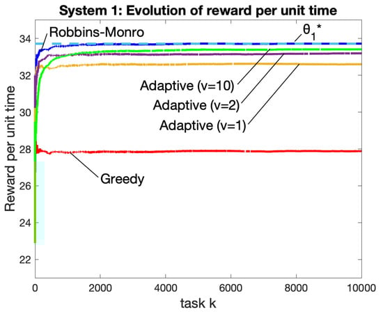
Figure 2. System 1 and Distribution 1: Accumulated reward per unit time for the proposed adaptive algorithm (with $v\in \{1,2,10\}$), the vanishing-stepsize Robbins–Monro algorithm, and the greedy algorithm. All data points are averaged over 40 independent simulations. The dashed horizontal line is the optimal ${\theta }_1^{*}$ for Distribution 1.

It can be seen that the greedy algorithm has significantly worse performance compared with the others. The Robbins–Monro algorithm, which uses a vanishing stepsize, has the fastest convergence and the highest achieved reward per unit time. As predicted by our theorems, the proposed adaptive algorithm has a convergence time that gets slower as v is increased, with a corresponding tradeoff in accuracy, where accuracy relates to the proximity of the converged value to the optimal ${\theta }^{*}$. The case $v=1$ converges quickly but has less accuracy. The cases $v=2$ and $v=10$ have accuracy that is competitive with Robbins–Monro.

Figure 3 illustrates the adaptation advantages of the proposed algorithm. Figure 3 considers simulations over $2\times {10}^4$ tasks. The first half of the simulation refers to tasks $\{1,\dots ,{10}^4\}$, the second half refers to tasks $\{{10}^4+1,\dots ,2\times {10}^4\}$. The $\left\{A\right[k\left]\right\}$ matrices in the first half are i.i.d. with Distribution 1; in the second half, they are i.i.d. with Distribution 2. Nobody tells the algorithms that a change occurs at the halfway mark; rather, the algorithms must adapt. The two dashed horizontal lines represent optimal ${\theta }^{*}$ values for Distribution 1 and Distribution 2. Data in Figure 3 is plotted as a moving average with a window of the past 200 tasks (and averaged over 40 independent simulations). As seen in the figure, the adaptive algorithm (with $v=10$) produces near-optimal performance that quickly adapts to the change. In stark contrast, the Robbins–Monro algorithm adapts very slowly to the change and takes roughly $(3/4)\times {10}^4$ tasks to move close to optimality. The adaptation time of Robbins–Monro is much slower than its convergence time starting at task 1. This is due to the vanishing stepsize and the fact that, at the time of the distribution change, the stepsize is very small. Theoretically, the Robbins–Monro algorithm has an arbitrarily large adaptation time, as can be seen by imagining a simulation that uses a fixed distribution for a number of tasks x before changing to another distribution: The stepsize at the time of change is $\eta \left[x\right]=1/(x+1)$, hence an arbitrarily large value of x yields an arbitrarily large adaptation time.

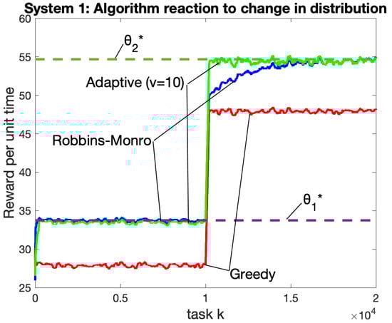
Figure 3. System 1: Testing adaptation over a simulation of $2\times {10}^4$ tasks with a distributional change introduced at the halfway point (task ${10}^4$). The two horizontal dashed lines represent optimal ${\theta }^{*}$ values for the two distributions. Each point for task k is the result of a moving window average ${\displaystyle \frac{{\sum }_{i=1}^{200}\mathbb{E}\left[R[k-i]\right]}{{\sum }_{i=1}^{200}\mathbb{E}\left[T[k-i]\right]}}$, where expectations are obtained by averaging over 40 independent simulations. The adaptive algorithm (with $v=10$) quickly adapts to the change. The Robbins–Monro algorithm takes a long time to adapt.

Figure 3 shows the greedy algorithm adapts very quickly. This is because the greedy algorithm maximizes $R\left[k\right]/T\left[k\right]$ for each task k without regard to history. Of course, the greedy algorithm is the least accurate and produces results that are significantly less than optimal for both distributions. To avoid clutter, the adaptive algorithm for cases $v=1,v=2$ are not plotted in Figure 3. Only the case $v=10$ is shown because this case has the slowest adaptation but the most accuracy (as compared with $v=1,v=2$ cases). While not shown in Figure 3, it was observed that the accuracy of the $v=2$ case was only marginally worse than that of the $v=10$ case (similar to Figure 2).

For the simulation of the proposed algorithm for the scenario of Figure 3, the virtual queue $J\left[k\right]$ was observed to have a maximum value $661.0219$ over the entire timeline, with a noticeable jump in average value of $J\left[k\right]$ after the midway point in the simulation, as shown in Figure 4.

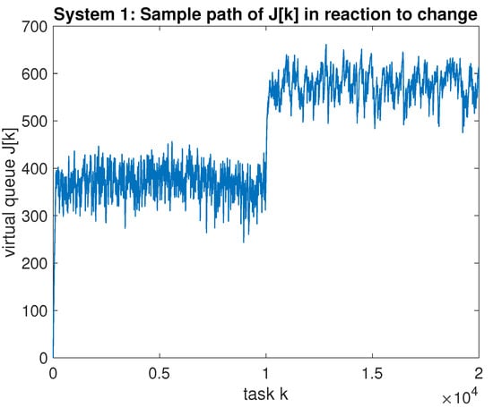
Figure 4. System 1: A sample path of virtual queue $J\left[k\right]$ for the proposed algorithm for the same scenario as Figure 3. A change in distribution occurs at the halfway point in the simulation.

The two distributions in this subsection (and in Figure 2, Figure 3 and Figure 4) are

• Distribution 1: With $M\left[k\right]$ being the random number of rows, we use $P\left[M\right[k]=1]=0.1$, $P\left[M\right[k]=2]=0.6$, $P\left[M\right[k]=3]=0.15$, $P\left[M\right[k]=4]=0.15$. The first row is always $[T_1,R_1]=[1,0]$ and represents a “vacation” option that lasts for one unit of time and has zero reward (as explained in [2], it can be optimal to take vacations a certain fraction of time, even if there are other row options). The remaining rows r, if any, have parameters $[T_r,R_r]$ generated independently with $T_r\sim Unif[1,10]$ and $R_r=T_r{G}_r$, where $G_r\sim Unif[0,50]$ and is independent of $T_r$.
• Distribution 2: We use $P\left[M\right[k]=1]=0$, $P\left[M\right[k]=2]=0.2$, $P\left[M\right[k]=3]=0.4$, $P\left[M\right[k]=4]=0.4$. The first row is always $[T_1,R_1]=[1,0]$. The other rows r are independently chosen as a random vector $[T_r,R_r]$ with $T_r\sim Unif[1,10]$, $R_r=G_r{T}_r+H_r$ with $G_r,H_r$ independent and $G_r\sim Unif[10,30]$, $H_r\sim Unif[0,200]$.

6.2. System 2

This subsection considers a device that processes computational tasks with the goal of maximizing time average profit subject to a time average power constraint of $p_{av}=1/3$ energy/time. There is a penalty process $Y\left[k\right]$ and so the Robbins–Monro algorithm of [2] cannot be used. For simplicity, we use $q_1=\infty$ (as discussed in Section 7). $Q_1\left[t\right]$ was observed to be stable with a maximum size of less than 350 over all time. We compare the adaptive algorithm of the current paper to the drift-plus-penalty ratio method of [6]. The ratio of expectations from the main method in [6] requires knowledge of the probability distribution on $A\left[k\right]$. A heuristic is proposed in Section VI.B in [6] that uses a drift-plus-penalty minimization of $-v\left(R\right[k]-\theta [k-1\left]T\right[k\left]\right)+Q\left[k\right]Y\left[k\right]$, which has a simple decision complexity for each task that is the same as the decision complexity of the adaptive algorithm proposed in the current paper, and where $\theta \left[k\right]$ is defined as a running average:

$$\theta \left[k\right]={\displaystyle \frac{{\sum }_{i=1}^{k}R\left[i\right]}{{\sum }_{i=1}^{k}T\left[i\right]}}$$

It is argued in Section VI.B in [6] that, if the heuristic converges, it converges to a point that is within $O\left(ϵ\right)$ of optimality, where the parameter v is chosen as $v=1/ϵ$. We call this heuristic “DPP with ratio averaging” in the simulations. (Another method described in [6] approximates the ratio of expectations using a window of w past samples. The per-task decision complexity grows with w and hence is larger than the complexity of the algorithm proposed in the current paper. For ease of implementation, we have not considered this method.) We also compare to a greedy method that removes any row r of $A\left[k\right]$ that does not satisfy $Energ{y}_r\left[k\right]/T_r\left[k\right]\le 1/3$, and chooses from the remaining rows to maximize $R_r\left[k\right]/T_r\left[k\right]$.

The i.i.d. matrices $\left\{A\right[k\left]\right\}$ have three columns and three rows of the form:

$$A\left[k\right]=\left[\begin{array}{ccc}1& 0& 0\\ T_2\left[k\right]& R_2\left[k\right]& Y_2\left[k\right]\\ T_3\left[k\right]& R_3\left[k\right]& Y_3\left[k\right]\end{array}\right]$$

where $Y_r\left[k\right]=Energ{y}_r\left[k\right]-(1/3)T_r\left[k\right]$ for $i\in \{2,3\}$. The first row corresponds ignoring task k and remaining idle for 1 unit of time, earning no reward but using no energy, so $(T_1\left[k\right],R_1\left[k\right],Y_1\left[k\right])=(1,0,0)$. The second row corresponds to processing task k at the home device. The third row corresponds to outsourcing task k to a cloud device. Two distributions are considered (specified at the end of this subsection). Under Distribution A, the reward is the same for both rows 2 and 3, but the energy and durations of time are different. Under Distribution B, the reward is higher for processing at the home device. Both distributions have $t_{min}=1$, $t_{max}=12$, $r_{max}=20$. We use $\alpha =c_1/max[c_2,1/2]$ for the adaptive algorithm. Under the distributions used, the greedy algorithm is never able to use row 2, can always use either row 1 or 3, and always selects row 3.

Figure 5 and Figure 6 consider reward and power for simulations over 5000 tasks with i.i.d. $\left\{A\right[k\left]\right\}$ under Distribution A. Figure 5 plots the running average of ${\displaystyle \frac{{\sum }_{i=1}^k\mathbb{E}\left[R\left[i\right]\right]}{{\sum }_{i=1}^k\mathbb{E}\left[T\left[i\right]\right]}}$ where expectations are attained by averaging over 40 independent simulations. The horizontal asymptote illustrates the optimal ${\theta }^{*}$ as obtained by simulation. The simulation uses $v=50$ for the DPP with ratio averaging because this was sufficient for an accurate approximation of ${\theta }^{*}$, as seen in Figure 5. The proposed adaptive algorithm is considered for $v=10,v=50,v=200$. As predicted by our theorems, it can be seen that the converged reward is closer to ${\theta }^{*}$ as v is increased (the case $v=200$ is competitive with DPP with ratio averaging). Figure 6 plots the corresponding running average of ${\displaystyle \frac{{\sum }_{i=1}^k\mathbb{E}\left[Energy\left[i\right]\right]}{{\sum }_{i=1}^k\mathbb{E}\left[T\left[i\right]\right]}}$. The disadvantage of choosing a large value of v is seen by the longer time required for time-averaged power to converge to the horizontal asymptote $p_{av}=1/3$. Figure 5 and Figure 6 show the greedy algorithm has the worst reward per unit time and has average power significantly under the required constraint. This shows that, unlike the other algorithms, the greedy algorithm does not make intelligent decisions for using more power to improve its reward. Considering only the performance shown in Figure 5 and Figure 6, the DPP with ratio averaging heuristic demonstrates the best convergence times, which is likely due to the fact that it uses only one virtual queue $Q\left[k\right]$ while our adaptive algorithm uses $Q\left[k\right]$ and $J\left[k\right]$. It is interesting to note that the adaptive algorithms and the DPP with ratio averaging heuristic both choose row 1 (idle) a significant fraction of the time. This is because, when a task has a small reward but a large duration of time, it is better to throw the task away and wait idly for a short amount of time in order to see a new task with a hopefully larger reward.

Figure 5. Time average reward up to task k for the proposed adaptive algorithm ($v\in \{10,50,200\}$); the DPP algorithm with ratio averaging; the greedy algorithm. The dashed horizontal line is the value ${\theta }_A^{*}$.

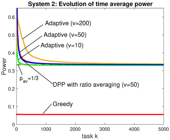
Figure 6. Corresponding time-averaged power for the simulations of Figure 5. The horizontal asymptote is $p_{av}=1/3$. The greedy algorithm falls too far under the $p_{av}$ constraint: it does not know how to use more power to increase its time average reward.

Significant adaptation advantages of our proposed algorithm are illustrated in Figure 7. Performance is plotted over a moving average with window size $w=200$, and averaged over 100 independent simulations. The first half of the simulation uses i.i.d. $\left\{A\right[k\left]\right\}$ with Distribution A, the second half uses Distribution B. The two horizontal asymptotes in Figure 7 are optimal ${\theta }_A^{*}$ and ${\theta }_B^{*}$ values for Distributions A and B. As seen in the figure, both the adaptive algorithm and the DPP with ratio averaging heuristic quickly converge to the optimal ${\theta }_A^{*}$ value associated with Distribution A (the rewards under the adaptive algorithm are slightly less than those of the heuristic). At the time of change, the adaptive algorithm has a spike that lasts for roughly 2000 tasks until it settles down to ${\theta }_B^{*}$. This can be viewed as the adaptation time and can be decreased by decreasing the value of v (at a corresponding accuracy cost). It converges from above to ${\theta }_B^{*}$ because, as seen in Figure 7, the spike marks a period of using more power than the required amount. In contrast, the DPP with ratio averaging algorithm cannot adapt and never increases to the optimal value of ${\theta }_B^{*}$.

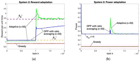
Figure 7. Adaptation for (a) reward and (b) power when the distribution is changed halfway through the simulation. Horizontal asymptotes are ${\theta }_A^{*}$ and ${\theta }_B^{*}$ for Distributions A and B. The adaptive algorithm settles into the new optimality point ${\theta }_B^{*}$, while DPP with ratio averaging cannot adapt.

The distributions used are as follows: For each task k, there are two independent random variables $U_1\left[k\right],U_2\left[k\right]\sim Unif[0,1]$ generated. Then,

• Distribution A: Note that $R_2\left[k\right]=R_3\left[k\right]$ and $T_2\left[k\right]<T_3\left[k\right]$ always.

  $$\begin{array}{cc}\hfill & (T_2\left[k\right],R_2\left[k\right],Energ{y}_2\left[k\right])=(1+9U_1\left[k\right],10U_1\left[k\right](U_2\left[k\right]+1),1+9U_1\left[k\right])\hfill \\ \hfill & (T_3\left[k\right],R_3\left[k\right],Energ{y}_3\left[k\right])=(6+6U_1\left[k\right],10U_1\left[k\right](U_2\left[k\right]+1),U_1\left[k\right])\hfill \end{array}$$
• Distribution B: The $R_2\left[k\right]$ value is increased in comparison to Distribution A.

  $$\begin{array}{cc}\hfill & (T_2\left[k\right],R_2\left[k\right],Energ{y}_2\left[k\right])=(1+9U_1\left[k\right],min\{20(U_2\left[k\right]+1),20\},1+9U_1\left[k\right])\hfill \\ \hfill & (T_3\left[k\right],R_3\left[k\right],Energ{y}_3\left[k\right])=(6+6U_1\left[k\right],10U_1\left[k\right](U_2\left[k\right]+1),U_1\left[k\right])\hfill \end{array}$$

6.3. Weight Adjustment

While the $\Theta (1/{ϵ}^2)$ adaptation times achieved by the proposed algorithm are asymptotically optimal, an important question is whether the coefficient can be improved by some constant factor. Specifically, this subsection attempts to reduce the 2000-task adaptation time seen in the spikes of Figure 7 and Figure 8 without degrading accuracy. We observe that the $J\left[k\right]$ and $Y\left[k\right]$ queues are weighted equally in the Lyapunov function $L\left[k\right]={\displaystyle \frac{1}{2}}J{\left[k\right]}^2+{\displaystyle \frac{1}{2}}Y{\left[k\right]}^2$. More weight can be placed on $Y\left[k\right]$ to emphasize the average power constraint and thereby reduce the spike in Figure 8b. This can be performed with no change in the mathematical analysis by redefining the penalty as $Y^{\prime }\left[k\right]=wY\left[k\right]$ for some constant $w>0$. The constraint $\overline{Y}\le 0$ is the same as ${\overline{Y}}^{\prime }\le 0$. We use $w=2$ and also double the v parameter from 50 to 100, which maintains the same relative weight between reward and $Q\left[k\right]$ but deemphasizes the $J\left[k\right]$ virtual queue by a factor of 2.

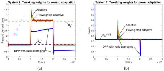
Figure 8. Comparing (a) reward and (b) power of the reweighted adaptive scheme when the distribution changes twice. Parameters for the adaptive and DPP with ratio averaging algorithms are the same as Figure 7.

Figure 8 plots performance over $3\times {10}^4$ tasks with Distribution A in the first third, Distribution B in the second third, and Distribution A in the final third. The adaptive algorithm and the DPP with ratio averaging algorithm use the same parameters as in Figure 7. The reweighted adaptive algorithm uses $v=100$ and $Y^{\prime }\left[k\right]=2Y\left[k\right]$. It can be seen that the reweighting decreases adaptation time with no noticeable change in accuracy. This illustrates the benefits of weighting the power penalty $Y\left[k\right]$ more heavily than the virtual queue $J\left[k\right]$.

The simulations in Figure 8 further show that the proposed adaptive algorithms can effectively handle multiple distributional changes. Indeed, the reward settles close to the new optimality point after each change in distribution. In contrast, the DPP with ratio averaging algorithm, which was not designed to be adaptive, appears completely lost after the first distribution change and never recovers. This emphasizes the importance of adaptive algorithms.

The value of the virtual queue $Q\left[k\right]$ for the proposed algorithm and its reweighted variant are shown in Figure 9. This illustrates that using $q_1=\infty$, which puts no deterministic upper bound on $Q\left[k\right]$, does not adversely affect performance, as discussed in Section 7. The virtual queue $J\left[k\right]$ is not shown, but its behavior is similar, and its maximum value over all time was observed to be less than 400.

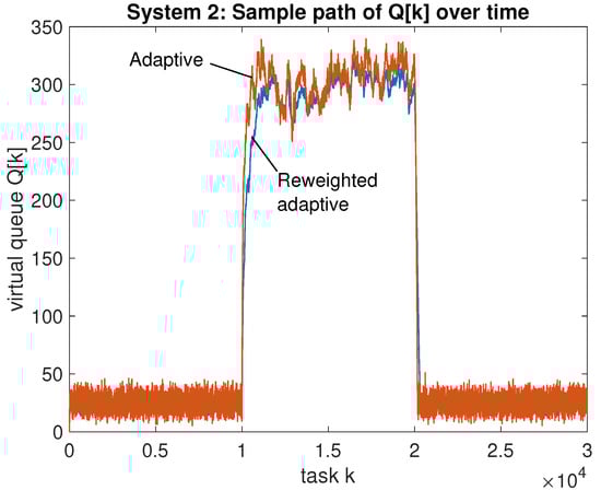
Figure 9. System 2: A sample path of $Q\left[k\right]$ for the proposed adaptive algorithm and its reweighted variant for the same scenario as Figure 8.

7. Discussion

The proposed algorithm can be run indefinitely over an infinite sequence of tasks. The analysis holds for any block of m tasks over which $\left\{A\right[k\left]\right\}$ is i.i.d. over that block. This holds regardless of sample path history before the block. A useful mathematical model that fits our analysis is when $\left\{A\right[k\left]\right\}$ evolves over disjoint and variable-length blocks of time during which behavior is i.i.d. with a fixed but unknown distribution, and where the start and end times of each block are unknown. In this scenario, the algorithm adapts and comes within $\Theta \left(ϵ\right)$ of optimality for every block that lasts for at least $1/{ϵ}^2$ tasks.

What happens if $\left\{A\right[k\left]\right\}$ is not i.i.d. over a block of interest? The good news is that our analysis provides worst-case bounds on the virtual queues that hold for all time and for any sample path. This means the algorithm maintains reasonable operational states. Of course, our optimality analysis uses the i.i.d. assumption. We conjecture that the algorithm also makes efficient decisions in more general situations where $\left\{A\right[k\left]\right\}$ arises from an ergodic Markov chain. The analysis in that situation would be more complicated, and the adaptation times would depend on the mixing time of the Markov process. We leave such open questions for future work.

There are situations where $\left\{A\right[k\left]\right\}$ evolves according to an ergodic Markov chain with very slow mixing times, slower than any reasonable timescale over which we want our algorithm to adapt. For example, one can imagine a 2-state Markov chain where $A\left[k\right]$ is i.i.d. with one distribution in state 1, and i.i.d. with another distribution in state 2. If transition probabilities between states 1 and 2 are very small, then state transitions may occur on a timescale of hours (and ergodic mixing times may be on the order of days or weeks), while thousands of tasks are performed before each state transition. Each state transition starts a new block of tasks. Our algorithm adapts to each new distribution, without knowing the transition times, provided that transition times are separated by at least $1/{ϵ}^2$ tasks. In other words, our convergence analysis holds on the shorter timescale of the block, rather than the longer (and possibly irrelevant) mixing time of the underlying Markov chain.

When $n>0$, the algorithm has a parameter $q_1>0$, where $q_1=\Theta \left(1\right)$. Theorem 2 suggests $q_1\ge 2d_0/s$. This requires knowledge of $d_0/s$. In practice, there is little danger in choosing $q_1$ to be too large. Even choosing $q_1=\infty$ works well in practice (see simulation section). Intuitively, this is because the virtual queue update (27) for $q_1=\infty$ reduces to

$$Q_i[k+1]=max\left\{Q_i\left[k\right]+Y_i\left[k\right],0\right\}\forall k\in \{1,2,3,\dots \}$$

which means $1_i\left[k\right]=0$ for all k and the inequality (30) can be modified to

$${\displaystyle \frac{1}{m}}{\sum }_{k=k_0}^{k_0+m-1}{Y}_i\left[k\right]\le {\displaystyle \frac{Q_i[k_0+m]-Q_i\left[k_0\right]}{m}}$$

(82)

for all positive integers $k_0,m$. Intuitively, the Slater condition still ensures $\left|\right|Q\left[k\right]\left|\right|$ concentrates quickly and is still rarely much larger than the $\lambda$ parameter in Lemma 7, where $\lambda =\Theta \left(v\right)$. Intuitively, while the $J\left[k\right]$ virtual queue would no longer be deterministically bounded, it would stay within its existing bounds with high probability. Taking expectations of (82) would then produce a right-hand side proportional to $v/m$, which is $O\left(ϵ\right)$ whenever $v=\Theta (1/ϵ)$ and $m\ge 1/{ϵ}^2$.

8. Conclusions

This paper gives an adaptive algorithm for renewal optimization, where decisions for each task k determine the duration of the task, the reward for the task, and a vector of penalties. The algorithm has a low per-task decision complexity, operates without knowledge of system probabilities, and is robust to changes in the probability distribution that occur at unknown times. A new hierarchical decision rule enables the algorithm to achieve within $ϵ$ of optimality over any sequence of $\Theta (1/{ϵ}^2)$ tasks over which the probability distribution is fixed, regardless of system history. This adaptation time matches a prior converse result that shows any algorithm that guarantees $ϵ$-optimality during tasks $\{1,\dots ,m\}$ must have $m\ge \Omega (1/{ϵ}^2)$, even if there are no additional penalty processes.

References

- Neely, M.J. Stochastic Network Optimization with Application to Communication and Queueing Systems; Morgan & Claypool: San Rafael, CA, USA, 2010. [Google Scholar]
- Neely, M.J. Fast Learning for Renewal Optimization in Online Task Scheduling. J. Mach. Learn. Res. 2021, 22, 1–44. [Google Scholar]
- Fox, B. Markov Renewal Programming by Linear Fractional Programming. SIAM J. Appl. Math. 1966, 14, 1418–1432. [Google Scholar] [CrossRef]
- Boyd, S.; Vandenberghe, L. Convex Optimization; Cambridge University Press: Cambridge, UK, 2004. [Google Scholar]
- Neely, M.J. Online Fractional Programming for Markov Decision Systems. In Proceedings of the 2011 49th Annual Allerton Conference on Communication, Control, and Computing (Allerton), Monticello, IL, USA, 28–30 September 2011. [Google Scholar]
- Neely, M.J. Dynamic Optimization and Learning for Renewal Systems. IEEE Trans. Autom. Control 2013, 58, 32–46. [Google Scholar] [CrossRef]
- Tassiulas, L.; Ephremides, A. Dynamic Server Allocation to Parallel Queues with Randomly Varying Connectivity. IEEE Trans. Inf. Theory 1993, 39, 466–478. [Google Scholar] [CrossRef]
- Tassiulas, L.; Ephremides, A. Stability Properties of Constrained Queueing Systems and Scheduling Policies for Maximum Throughput in Multihop Radio Networks. IEEE Trans. Autom. Control 1992, 37, 1936–1948. [Google Scholar] [CrossRef]
- Wei, X.; Neely, M.J. Data Center Server Provision: Distributed Asynchronous Control for Coupled Renewal Systems. IEEE/ACM Trans. Netw. 2017, 25, 2180–2194. [Google Scholar] [CrossRef]
- Wei, X.; Neely, M.J. Asynchronous Optimization over Weakly Coupled Renewal Systems. Stoch. Syst. 2018, 8, 167–191. [Google Scholar] [CrossRef]
- Robbins, H.; Monro, S. A Stochastic Approximation Method. Ann. Math. Stat. 1951, 22, 400–407. [Google Scholar] [CrossRef]
- Borkar, V.S. Stochastic Approximation: A Dynamical Systems Viewpoint; Springer: Berlin/Heidelberg, Germany, 2008. [Google Scholar]
- Nemirovski, A.; Yudin, D. Problem Complexity and Method Efficiency in Optimization; Wiley-Interscience Series in Discrete Mathematics; John Wiley: Hoboken, NJ, USA, 1983. [Google Scholar]
- Kushner, H.J.; Yin, G. Stochastic Approximation and Recursive Algorithms and Applications; Springer: Berlin/Heidelberg, Germany, 2003. [Google Scholar]
- Toulis, P.; Horel, T.; Airoldi, E.M. The Proximal Robbins–Monro Method. J. R. Stat. Soc. Ser. B Stat. Methodol. 2021, 83, 188–212. [Google Scholar] [CrossRef]
- Nemirovski, A.; Juditsky, A.; Lan, G.; Shapiro, A. Robust Stochastic Approximation Approach to Stochastic Programming. SIAM J. Optim. 2009, 19, 1574–1609. [Google Scholar] [CrossRef]
- Joseph, V.R. Efficient Robbins-Monro Procedure for Binary Data. Biometrika 2004, 91, 461–470. [Google Scholar] [CrossRef]
- Zinkevich, M. Online convex programming and generalized infinitesimal gradient ascent. In Proceedings of the 20th International Conference on Machine Learning (ICML), Washington, DC, USA, 21–24 August 2003. [Google Scholar]
- Huo, D.L.; Chen, Y.; Xie, Q. Bias and Extrapolation in Markovian Linear Stochastic Approximation with Constant Stepsizes. In Proceedings of the Abstract Proceedings of the 2023 ACM SIGMETRICS International Conference on Measurement and Modeling of Computer Systems (SIGMETRICS ’23), New York, NY, USA, 19–23 June 2023; pp. 81–82. [Google Scholar] [CrossRef]
- Luo, H.; Zhang, M.; Zhao, P. Adaptive Bandit Convex Optimization with Heterogeneous Curvature. Proc. Mach. Learn. Res. 2022, 178, 1–37. [Google Scholar]
- Van der Hoeven, D.; Cutkosky, A.; Luo, H. Comparator-Adaptive Convex Bandits. In Proceedings of the 34th International Conference on Neural Information Processing Systems (NIPS’20), Red Hook, NY, USA, 6–12 December 2020. [Google Scholar]
- Leyffer, S.; Menickelly, M.; Munson, T.; Vanaret, C.W.; Wild, S. A Survey of Nonlinear Robust Optimization. INFOR Inf. Syst. Oper. Res. 2020, 58, 342–373. [Google Scholar] [CrossRef]
- Tang, J.; Fu, C.; Mi, C.; Liu, H. An interval sequential linear programming for nonlinear robust optimization problems. Appl. Math. Model. 2022, 107, 256–274. [Google Scholar] [CrossRef]
- Badanidiyuru, A.; Kleinberg, R.; Slivkins, A. Bandits with Knapsacks. J. ACM 2018, 65, 1–55. [Google Scholar] [CrossRef]
- Agrawal, S.; Devanur, N.R. Bandits with Concave Rewards and Convex Knapsacks. In Proceedings of the Fifteenth ACM Conference on Economics and Computation (EC ’14), New York, NY, USA, 8–12 June 2014; pp. 989–1006. [Google Scholar] [CrossRef]
- Xia, Y.; Ding, W.; Zhang, X.; Yu, N.; Qin, T. Budgeted Bandit Problems with Continuous Random Costs. In Proceedings of the ACML, Hong Kong, 20–22 November 2015. [Google Scholar]
- Kallenberg, O. Foundations of Modern Probability, 2nd ed.; Probability and Its Applications; Springer: Berlin/Heidelberg, Germany, 2002. [Google Scholar]
- Neely, M.J. Energy-Aware Wireless Scheduling with Near Optimal Backlog and Convergence Time Tradeoffs. IEEE/ACM Trans. Netw. 2016, 24, 2223–2236. [Google Scholar] [CrossRef]
Disclaimer/Publisher’s Note: The statements, opinions and data contained in all publications are solely those of the individual author(s) and contributor(s) and not of MDPI and/or the editor(s). MDPI and/or the editor(s) disclaim responsibility for any injury to people or property resulting from any ideas, methods, instructions or products referred to in the content. |
© 2025 by the author. Licensee MDPI, Basel, Switzerland. This article is an open access article distributed under the terms and conditions of the Creative Commons Attribution (CC BY) license (https://creativecommons.org/licenses/by/4.0/).