An Advanced Hybrid Optimization Algorithm for Vehicle Suspension Design Using a QUBO-SQP Framework

Abstract

The design of multi-link vehicle suspension systems, such as the 3D double-wishbone, presents a critical challenge in automotive engineering. The process constitutes a high-dimensional, nonlinearly constrained optimization problem where traditional gradient-based methods often fail by converging to suboptimal local minima. This paper introduces a novel two-stage hybrid optimization framework designed to overcome this limitation by intelligently integrating quantum-inspired and classical techniques. The methodology explicitly defines a QUBO (Quadratic Unconstrained Binary Optimization) stage and an SQP (Sequential Quadratic Programming) stage. Stage 1 addresses the complex kinematic constraint problem by formulating it as a QUBO, which is then solved using Simulated Annealing to perform a global search, guaranteeing a physically feasible starting point. Subsequently, Stage 2 takes this feasible solution and employs an SQP algorithm to perform a high-precision local refinement, tuning the geometry to meet specific performance targets for camber and caster curves. The framework successfully converged to a design with a near-zero performance objective of 7.08 × 10⁻¹⁴. The efficacy of this hybrid approach is highlighted by the dramatic improvement from the high-error initial solution found by Simulated Annealing to the final, high-precision result from the SQP refinement. We conclude that this QUBO-SQP framework is a powerful and validated methodology for solving complex, real-world engineering design problems, effectively bridging the gap between global exploration and local precision.

1. Introduction

The dynamic behavior of a ground vehicle is the primary determinant of its handling precision, ride comfort, and overall safety. The suspension system, a nonlinear multi-body mechanism, plays a central role in mediating the force exchange between the vehicle chassis and the road surface. Among the various designs, the double-wishbone suspension is preeminent in high-performance and racing applications due to its superior control over wheel kinematics. By utilizing two lateral control arms, this configuration allows engineers to precisely tune key performance indicators (KPIs) such as camber gain, caster variation, and roll center height throughout the range of suspension travel [1]. However, this inherent design freedom introduces significant engineering complexity, making the task of optimizing the suspension’s geometric hardpoints a critical and high-value challenge in modern automotive engineering [2].

The core of the design challenge lies in its mathematical formulation [3]. The suspension geometry is defined by the three-dimensional coordinates of its chassis-side and upright-side pivot points, creating a high-dimensional design space. The physical relationships between these points are governed by a system of nonlinear trigonometric constraints, which must be satisfied for the mechanism to connect and move as intended [4]. Furthermore, the objective of matching specific kinematic performance curves (e.g., camber change with vertical wheel travel) results in a multi-modal objective function, where multiple local minima exist [5,6]. This makes global optimization particularly challenging, as traditional gradient-based solvers often converge to suboptimal solutions [7].

For such problems, two primary classes of algorithms have been applied to such problems. Gradient-based methods such as Sequential Quadratic Programming (SQP) are renowned for their computational efficiency and high-precision convergence but are sensitive to initial conditions [8]. Conversely, metaheuristics like Genetic Algorithms (GA) and Particle Swarm Optimization (PSO) offer robust global exploration but can be computationally expensive and lack refinement accuracy [9]. Hybrid methods have been proposed to address these limitations, combining surrogate models, Taguchi methods, and NSGA-II for improved hardpoint optimization [10].

Recent research highlights various strategies for improving double-wishbone suspension performance, from lightweight topology optimization of arms [11] to nonlinear stiffness modeling [6], finite element stress analysis [12], and comparative system-level evaluations [13]. Applications span motorcycles [14], ATVs [15], SUVs [16], and commercial vehicles [17].

To address the dichotomy between global and local optimization, this paper introduces a novel two-stage hybrid framework combining Quantum-Inspired Quadratic Unconstrained Binary Optimization (QUBO) with SQP refinement. This aligns with current efforts in surrogate-based and decoupled nonlinear modeling approaches that improve computational efficiency and solution robustness [4,10].

The remainder of this paper is structured as follows. Section 2 details the mathematical modeling of the 3D double-wishbone suspension, including the derivation of the kinematic constraints and performance objectives. Section 3 presents the architecture of the hybrid QUBO-SQP framework, detailing the formulation of the QUBO Hamiltonian and the role of each optimization stage. Section 4 presents the comprehensive results of the optimization, including a detailed analysis of the geometric changes, the kinematic performance improvement, and other key performance indicators that validate the methodology. Finally, Section 5 provides concluding remarks on the success of the framework and its potential impact on a broader class of complex engineering design problems.

2. System Modeling and Problem Formulation

This section establishes the complete mathematical model of the 3D double-wishbone suspension system. We define the geometric representation, derive the governing kinematic constraints, and formalize the performance objectives that constitute the optimization problem. The detailed vector-based formulation is provided in Appendix A.

2.1. Kinematic Model of the Double-Wishbone Suspension

The double-wishbone suspension is a spatial multi-body system. To analyze its motion, we first define its components, coordinate systems, and the mathematical tools to describe their relationship.

2.1.1. Geometric Hardpoints and Vectors

The geometry is defined by a set of physical hardpoints. From these, we derive a set of abstract vectors used in our optimization framework. The key components are the Upper Control Arm (UCA), Lower Control Arm (LCA), Upright (or knuckle), and Tie Rod (TR). Figure 1 illustrates these components and their defining hardpoints.

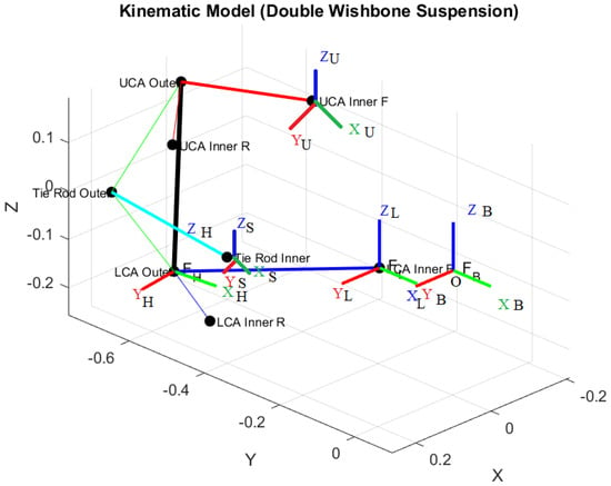
Figure 1. Schematic of the double-wishbone suspension model. The figure illustrates the spatial arrangement of the upper control arm (UCA), lower control arm (LCA), tie-rod, hub, and associated coordinate frames. The colors indicate coordinate axes and linkages for different components, red axes represent the local X-directions, green axes represent the Y-directions, and blue axes represent the Z-directions of each component frame.

The optimization variables are defined as follows:

• $o_{UB}$, $o_{LB}$, $o_{SB}$: Global coordinates of the front-inner chassis pivots for the UCA, LCA, and TR, respectively.
• $p_{\mathrm{RearU}}$, $p_{\mathrm{RearL}}$: Vectors from the front-inner to the rear-inner chassis pivots for the UCA and LCA.
• $o_{HL}$: Vector from the LCA inner pivot ($o_{LB}$) to the lower ball joint, defined in the LCA’s local frame.
• $p_{1H}$: Vector from the lower ball joint to the upper ball joint, defined in the Upright’s local frame.
• $p_{2H}$: Vector from the lower ball joint to the Tie Rod end, defined in the Upright’s local frame.
• $p_{1U}$: Vector from the UCA inner pivot ($o_{UB}$) to the upper ball joint, defined in the UCA’s local frame.
• $p_{2S}$: Vector from the TR inner pivot ($o_{SB}$) to the Tie Rod end, defined in the TR’s local frame.

2.1.2. Coordinate Systems

We define a global chassis frame, $\mathcal{B}=\{X,Y,Z\}$, which is fixed to the vehicle. X is longitudinal (positive forward), Y is lateral (positive left or right, by convention), and Z is vertical (positive upward). Each moving component (UCA, LCA, Upright, TR) also has its own local coordinate frame.

2.1.3. Mathematical Tools: Homogeneous Transformation Matrices

The orientation and position of any local frame relative to the global frame can be described by a $4\times 4$ Homogeneous Transformation (HT) matrix, T. An HT matrix combines a $3\times 3$ rotation matrix R and a $3\times 1$ translation vector p. A point $P_{\mathrm{local}}$ in a local frame can be transformed to its global coordinates $P_{\mathrm{global}}$ using the transformation as follows:

$$P_{\mathrm{global}}=T{P}_{\mathrm{local}}$$

(1)

where P is a homogeneous coordinate vector ${[x,y,z,1]}^{\mathrm{T}}$. The HT matrix is constructed as

$$T=\left[\begin{array}{cc}R& p\\ 0& 1\end{array}\right]$$

(2)

where R is the rotation matrix corresponding to the component’s orientation (defined by Euler angles $\varphi$, $\theta$, $\psi$ for roll, pitch, yaw) and p is the origin of the local frame in global coordinates.

2.2. Loop-Closure Constraints

For the suspension to be a connected mechanism, the vector chains from the chassis to the upright must be equal, regardless of the path taken. This principle gives rise to two fundamental loop-closure equality constraints that must hold true for all points in the suspension’s travel.

2.2.1. Upper Control Arm (UCA) Loop

The position of the upper ball joint can be reached from the chassis either directly via the UCA or by traversing through the LCA and then up the upright. These two paths must result in the same global coordinate. This is expressed as

$$\begin{array}{c}\mathrm{Global}\left(o_{UB}\right)+T_{\mathrm{UCA}}·\mathrm{Local}\left(p_{1U}\right)=\\ \mathrm{Global}\left(o_{LB}\right)+T_{\mathrm{LCA}}·\mathrm{Local}\left(o_{HL}\right)+T_{\mathrm{LCA}}·T_{\mathrm{Upright}}·\mathrm{Local}\left(p_{1H}\right)\end{array}$$

Using the state vector $q=[p;\Theta ]$ (where $\Theta$ is the Euler angle vector) and the HT matrix $T=\mathrm{HT}\left(q\right)$, this constraint is formalized as

$$h_1=\mathrm{HT}\left(q_u\right){\overline{p}}_{1u}-\mathrm{HT}\left(q_l\right)\mathrm{HT}\left(q_h\right){\overline{p}}_{1h}=0$$

(3)

where $\overline{p}$ denotes the homogeneous coordinate vector (i.e., the vector padded with a final coordinate of 1).

2.2.2. Tie Rod (TR) Loop

Similarly, the position of the Tie Rod’s outer end can be reached directly via the Tie Rod or through the LCA and Upright. This forms the second constraint:

$$h_2=\mathrm{HT}\left(q_s\right){\overline{p}}_{2s}-\mathrm{HT}\left(q_l\right)\mathrm{HT}\left(q_h\right){\overline{p}}_{2h}=0$$

(4)

These two vector equations, $h_1$ and $h_2$, represent six scalar equality constraints ($x,y,z$ for each) that must be satisfied by the optimizer.

2.3. Performance Objectives

The goal of the optimization is to control the orientation of the wheel as it moves. The two primary performance metrics are camber and caster angles. These are defined by the total rotation matrix from the global chassis frame to the hub frame, $R_{\mathrm{HB}}$. This matrix is calculated by composing the rotations of the LCA and the Upright:

$$R_{\mathrm{HB}}=R_{\mathrm{LCA}}^{\mathrm{T}}{R}_{\mathrm{Upright}}^{\mathrm{T}}$$

(5)

2.4. Camber Angle (γ)

It is defined as the inclination of the wheel from the vertical axis, viewed from the front. It is the rotation about the vehicle’s longitudinal (X) axis. It can be extracted directly from the rotation matrix $R_{\mathrm{HB}}$:

$$\gamma =arcsin(-R_{\mathrm{HB}}(3,2))$$

(6)

2.5. Caster Angle (τ)

It is defined as the angle of the steering axis, viewed from the side. It is the rotation about the vehicle’s vertical (Z) axis. It is also extracted from $R_{\mathrm{HB}}$:

$$\tau =arctan2(R_{\mathrm{HB}}(1,2),R_{\mathrm{HB}}(2,2))$$

(7)

The optimizer’s goal is to match these calculated angles to predefined target functions that depend on the suspension’s roll angle (${\varphi }_{\mathrm{LCA}}$):

$$\begin{array}{cc}\hfill {\gamma }_{\mathrm{Target}}& =f\left({\varphi }_{\mathrm{LCA}}\right)=-1.5°-0.2·{\varphi }_{\mathrm{LCA}}\hfill \end{array}$$

(8)

$$\begin{array}{cc}\hfill {\tau }_{\mathrm{Target}}& =g\left({\varphi }_{\mathrm{LCA}}\right)=8.0°+0.1·{\varphi }_{\mathrm{LCA}}\hfill \end{array}$$

(9)

2.6. The Formal Optimization Problem

Combining the objectives and constraints, we can now state the complete, formal optimization problem. Let the design vector x contain all the geometric vectors and the state variables (joint angles) for n points of suspension travel. The problem is to find the optimal design vector $x^{*}$ that solves the following:

Minimize

$$J\left(x\right)=\sum _{i=1}^n\left[w_{\gamma }{(\gamma {\left(x\right)}_i-{\gamma }_{\mathrm{Target},i})}^2+w_{\tau }{(\tau {\left(x\right)}_i-{\tau }_{\mathrm{Target},i})}^2\right]$$

(10)

Subject to

$$\begin{array}{cc}\hfill h_1{\left(x\right)}_i& =0\mathrm{for}i=1\dots n\hfill \end{array}$$

(11)

$$\begin{array}{cc}\hfill h_2{\left(x\right)}_i& =0\mathrm{for}i=1\dots n\hfill \end{array}$$

(12)

where $w_{\gamma }$ and $w_{\tau }$ are weighting factors for the camber and caster objectives, respectively. This formalizes the multi-point, nonlinearly constrained optimization problem that we solve using our hybrid framework.

3. The Hybrid QUBO-SQP Optimization Framework

To solve the complex problem defined in Section 2, we introduce a two-stage hybrid optimization framework. This methodology is explicitly designed to overcome the limitations of using a single optimization technique by strategically decoupling the problem into two distinct tasks: a global search for a physically feasible design, followed by a local search for a high-performance refined design. This section details the architecture and mathematical formulation of each stage.

3.1. Framework Overview

The core principle of our framework is to use a quantum-inspired approach to solve the most challenging part of the problem satisfying the nonlinear kinematic constraints and then use a highly efficient classical algorithm to tune the resulting valid design for performance. The data flow, illustrated in Figure 2, is a sequential process where the output of the first stage serves as the input for the second.

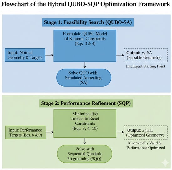
Figure 2. Flowchart of the proposed two-stage hybrid QUBO-SQP optimization framework.

• Input: The process begins with the nominal (initial) suspension geometry and the desired performance targets.
• Stage 1: Feasibility Search (QUBO-SA): The continuous design space is discretized into a binary representation. The nonlinear kinematic constraints (Equations (3) and (4)) are approximated as a quadratic polynomial of binary variables, forming a QUBO model. The QUBO is solved using a Simulated Annealer (SA) to find a binary solution that minimizes the constraint violation. This binary solution is decoded back into a continuous vector, $x_{0\_\mathrm{SA}}$. This vector represents a physically feasible, but not yet performance-optimized, suspension geometry.
• Stage 2: Performance Refinement (SQP): The feasible vector $x_{0\_\mathrm{SA}}$ is used as the initial guess for the Sequential Quadratic Programming (SQP) optimizer. The SQP algorithm minimizes the high-precision performance objective (Equation (10)) subject to the exact, non-approximated trigonometric constraints (Equations (3) and (4)).
• Output: The final output, $x_{\mathrm{final}}$, is a suspension geometry that is both kinematically valid and performance-optimized.

3.2. Stage 1: QUBO Formulation for Feasibility Search

The objective of Stage 1 is to find a point in the vast, high-dimensional design space that satisfies the fundamental laws of physics for the mechanism, i.e., a point where the loop-closure constraints are met. Further details on the QUBO model size and sparsity are provided in Appendix B.

3.2.1. Discretization of Continuous Variables

The QUBO model operates exclusively on binary variables ($b_i\in \{0,1\}$). Therefore, each continuous design variable v in our model (e.g., a coordinate or an angle) must be mapped to a set of $N_b$ binary variables. We define a search range for each variable v from $v_{min}$ to $v_{max}$. The continuous variable is then expressed as a function of its $N_b$ binary variables $\{b_0,b_1,\dots ,b_{N_b-1}\}$ using the standard binary encoding:

$$v\approx v_{min}+(v_{max}-v_{min})·\left({\displaystyle \frac{1}{2^{N_b}-1}}\right)\sum _{i=0}^{N_b-1}{2}^i{b}_i$$

(13)

This transformation converts the entire continuous design space into a discrete combinatorial space that the QUBO can operate on.

3.2.2. Polynomial Approximation of Constraints

The trigonometric functions $sin\left(\theta \right)$ and $cos\left(\theta \right)$ in the kinematic constraints (Equations (3) and (4)) are transcendental and cannot be directly represented in a QUBO, which is inherently a quadratic polynomial. To overcome this, we employ a Taylor series expansion around $\theta =0$, which is valid for the small angles of rotation expected in suspension components. We use a first-order approximation for sine and a second-order approximation for cosine:

$$\begin{array}{cc}\hfill sin\left(\theta \right)& \approx \theta \hfill \end{array}$$

(14)

$$\begin{array}{cc}\hfill cos\left(\theta \right)& \approx 1-{\displaystyle \frac{{\theta }^2}{2}}\hfill \end{array}$$

(15)

By substituting these approximations into the rotation matrices within our kinematic model, the complex constraints of Equations (3) and (4) are transformed into a system of quadratic polynomials of the discretized variables. Let these approximated constraint vectors be denoted by ${\tilde{h}}_1$ and ${\tilde{h}}_2$.

3.2.3. Hamiltonian Construction

The objective function of a QUBO is called a Hamiltonian, H. In our framework, the Hamiltonian is constructed to be an energy function where the lowest energy state corresponds to the best possible satisfaction of the physical constraints. We define it as the weighted sum of the squared norms of the approximated constraint vectors, summed over all n points of suspension travel:

$$H\left(b\right)=w_c\sum _{i=1}^n\left[\left|\right|{\tilde{h}}_1{\left(b\right)}_i{\left|\right|}^2+\left|\right|{\tilde{h}}_2{\left(b\right)}_i{\left|\right|}^2\right]$$

(16)

where b is the vector of all binary variables and $w_c$ is a penalty weight. Crucially, this Hamiltonian is a function of only the constraint violations. The performance objectives (Equation (10)) are intentionally excluded from this stage. This focuses the solver on the singular task of finding a feasible solution. After expansion, $H\left(b\right)$ takes the canonical QUBO form:

$$H\left(b\right)=\sum _i{h}_i{b}_i+\sum _{i<j}{Q}_{ij}{b}_i{b}_j$$

(17)

where h represents the linear weights and Q is the quadratic coupling matrix.

3.2.4. Solver: Simulated Annealing (SA)

Finding the ground state (minimum value) of the Hamiltonian (Equation (17)) is an NP-hard problem. While quantum annealers are designed for this, highly effective classical algorithms exist. We employ Simulated Annealing, a metaheuristic inspired by the annealing process in metallurgy. SA iteratively explores the solution space, accepting uphill moves (solutions that temporarily increase the energy H) with a probability that decreases over time. This mechanism allows the algorithm to effectively escape poor local minima and find a solution in the region of the global minimum, making it an ideal choice for solving the QUBO on classical hardware.

3.3. Stage 2: SQP for Performance Refinement

The solution from Stage 1, $x_{0\_\mathrm{SA}}$, is a continuous vector that represents a physically valid, but not necessarily high-performing, suspension geometry. The purpose of Stage 2 is to take this intelligent starting guess and refine it to meet the performance targets with high precision.

3.3.1. Algorithm: Sequential Quadratic Programming (SQP)

We employ SQP, a powerful gradient-based algorithm for nonlinearly constrained optimization. At each iteration, SQP approximates the problem as a Quadratic Programming (QP) subproblem, which can be solved efficiently. It uses the gradients of both the objective function and the constraints to determine the optimal search direction, allowing for very rapid convergence once it is near a minimum.

3.3.2. Problem Formulation for SQP

The SQP solver is tasked with solving the original, full-precision problem defined in Section 2.1:

• Initial Guess: $x_0=x_{0\_\mathrm{SA}}$
• Objective Function: The exact performance objective $J\left(x\right)$ from Equation (10), using the precise sin and cos functions.
• Constraints: The exact loop-closure constraints $h_1\left(x\right)=0$ and $h_2\left(x\right)=0$ from Equations (3) and (4), again using precise trigonometry.

By providing SQP with a starting point that is already in a feasible region, we mitigate its primary weakness (sensitivity to the initial guess) and leverage its primary strength (fast, high-precision local convergence) (Algorithm 1).

Algorithm 1 The Hybrid QUBO-SQP Framework

Require: Nominal geometry $x_{\mathrm{nom}}$, Performance targets T Ensure: Optimized geometry $x_{\mathrm{final}}$   1: // Stage 1: Feasibility Search   2: Discretize continuous variables v into binary variables b using Equation (13).   3: Approximate kinematic constraints h to polynomials $\tilde{h}$ using Equations (14) and (15).   4: Construct QUBO Hamiltonian $H\left(b\right)$ from $\tilde{h}$ using Equation (16).   5: $b_{\mathrm{sol}}\leftarrow \mathrm{Simulated}\mathrm{Annealing}\left(H\right)$   6: Decode $b_{\mathrm{sol}}$ back to continuous vector $x_{0\_\mathrm{SA}}$ using Equation (13).   7:   8: // Stage 2: Performance Refinement   9: Set initial guess $x_0\leftarrow x_{0\_\mathrm{SA}}$.  10: Define objective $J\left(x\right)$ using Equation (10) (full precision).  11: Define constraints $h\left(x\right)$ using Equations (3) and (4) (full precision).  12: $x_{\mathrm{final}}\leftarrow \mathrm{SQP}(J,h,x_0)$  13: return  $x_{\mathrm{final}}$

4. Results and Discussion

The hybrid QUBO-SQP framework was implemented and executed to solve the 3D double-wishbone suspension optimization problem. This section presents the specific implementation details, quantifies the performance of the optimization process, and provides a detailed analysis of the final geometric and kinematic results.

4.1. Implementation Details

The entire optimization framework was implemented in the Python 3 programming language. The QUBO model in Stage 1 was constructed using the PyQUBO library, which allows for the symbolic definition of a Hamiltonian from binary variable expressions. The subsequent NP-hard QUBO problem was solved on classical hardware using the Simulated Annealer provided by the dwave-neal package. Stage 2 of the framework, the high-precision refinement, was performed using the Sequential Least Squares Programming (SLSQP) algorithm, a robust implementation of SQP available in the SciPy optimization library. All visualizations were generated using Matplotlib version 3.10.0.

The key hyperparameters for the Stage 1 feasibility search were chosen to balance computational cost with a sufficient search space resolution. The number of binary variables per continuous variable (NUM_BITS) was set to 1, allowing each design variable to be either at its minimum or maximum bound within a defined range. This INVESTIGATION_RANGE was set to ±5 mm from the nominal geometric coordinates. The kinematic constraints were evaluated at three distinct roll points (NP_POINTS) across a ±3° range of motion. The penalty weight $w_c$ in the Hamiltonian was set to $200.0$ to strongly enforce the satisfaction of constraints.

4.2. Optimization Performance and Convergence

The two-stage optimization process was executed on a standard desktop computer, demonstrating the framework’s efficiency and suitability for practical engineering workflows. The computational performance for each stage is summarized below:

4.2.1. Stage 1 (QUBO-SA Feasibility Search)

The compilation of the QUBO model from the symbolic Hamiltonian resulted in a system of 583 binary variables and 6752 quadratic couplings. The Simulated Annealer successfully found a low-energy solution for this system in $0.24\mathrm{s}$. The final energy of the returned solution was $-63.8842$, indicating that the solver found a binary configuration that significantly minimized the kinematic constraint violations.

4.2.2. Stage 2 (SQP Performance Refinement)

Sequential Quadratic Programming (SQP) stage solves the constrained optimization problem by iteratively minimizing a quadratic approximation of the Lagrangian function subject to linearized constraints. At each iteration, the SQP algorithm updates both the design variables and the associated Lagrange multipliers to ensure feasibility and optimality. In this work, the SLSQP implementation from the SciPy optimization library was employed, providing robustness for nonlinear mechanical systems and efficient convergence near constraint boundaries.

Using the decoded SA solution as its starting point, the SQP optimizer began its refinement process. The algorithm successfully converged to a solution in 15 iterations, which required 872 function evaluations and took $0.89\mathrm{s}$.

The final value of the performance objective function $J\left(x\right)$ after Stage 2 was $7.08\times {10}^{-14}$. A value of this magnitude is orders of magnitude below any practical engineering tolerance and is effectively zero, indicating a near-perfect convergence. This result confirms that the SQP optimizer, when guided by the feasible solution from Stage 1, was able to precisely match the suspension’s kinematic performance to the desired camber and caster target curves. The successful and rapid convergence of both stages validates the computational efficiency and overall efficacy of the proposed hybrid approach.

4.3. Analysis of Geometric Changes

To achieve the desired kinematic performance, the optimizer significantly altered the initial nominal geometry. Table 1 provides a direct comparison of the initial and final values for the abstract geometric vectors that define the suspension hard points.

Table 1. Comparison of initial and final optimized geometric variable values.

Variable	Axis	Initial (m)	Optimized (m)
$o_{UB}$	x	$-0.0800$	$-0.1357$
$o_{UB}$	y	$-0.4500$	$-0.4873$
$o_{UB}$	z	$0.1800$	$0.0287$
$o_{LB}$	x	$-0.1990$	$-0.2088$
$o_{LB}$	y	$-0.4000$	$-0.3543$
$o_{LB}$	z	$-0.1950$	$-0.1388$
$o_{SB}$	x	$0.2000$	$0.2505$
$o_{SB}$	y	$-0.4000$	$-0.4134$
$o_{SB}$	z	$-0.0450$	$0.0551$
$p_{1U}$	x	$0.1210$	$0.1467$
$p_{1U}$	y	$-0.2250$	$-0.0037$
$p_{1U}$	z	$0.0000$	$-0.0979$
$p_{1H}$	x	$0.0400$	$-0.0058$
$p_{1H}$	y	$0.0750$	$0.1329$
$p_{1H}$	z	$0.4250$	$0.0528$
$p_{2H}$	x	$0.1490$	$0.2481$
$p_{2H}$	y	$0.0000$	$0.0180$
$p_{2H}$	z	$0.2000$	$0.1620$
$p_{2S}$	x	$-0.0500$	$-0.0396$
$p_{2S}$	y	$-0.3500$	$-0.1681$
$p_{2S}$	z	$0.0000$	$-0.0496$
$o_{HL}$	x	$0.2000$	$0.1902$
$o_{HL}$	y	$-0.3500$	$-0.2671$
$o_{HL}$	z	$-0.0500$	$-0.0302$
$p_{\mathrm{RearU}}$	x	$0.3310$	$0.3310$
$p_{\mathrm{RearU}}$	y	$-0.0400$	$-0.0400$
$p_{\mathrm{RearU}}$	z	$0.0050$	$0.0050$
$p_{\mathrm{RearL}}$	x	$0.4000$	$0.4000$
$p_{\mathrm{RearL}}$	y	$-0.0500$	$-0.0500$
$p_{\mathrm{RearL}}$	z	$0.0050$	$0.0050$

While Table 1 shows the changes in the abstract vectors, Table 2 offers a more intuitive physical interpretation by quantifying the total Euclidean distance each hard point’s defining vector moved.

Table 2. Total displacement of each geometric vector from its initial to its final optimized state.

Variable	Displacement (mm)
$o_{UB}$	$165.23$
$o_{LB}$	$57.69$
$o_{SB}$	$114.21$
$p_{1U}$	$258.05$
$p_{1H}$	$376.19$
$p_{2H}$	$115.61$
$p_{2S}$	$185.34$
$o_{HL}$	$85.03$
$p_{\mathrm{RearU}}$	$0.00$
$p_{\mathrm{RearL}}$	$0.00$

The results from these tables are striking. The optimizer found a non-trivial solution that is substantially different from the starting geometry. The most significant change occurred in the $p_{1H}$ vector, which defines the upright’s geometry, moving by over $376\mathrm{mm}$. The UCA’s local vector $p_{1U}$ also underwent a massive change of $258\mathrm{mm}$. These large displacements underscore the difficulty of the problem; a simple manual or localized search around the initial design would have been highly unlikely to discover this distant, high-performance solution. This demonstrates the framework’s ability to navigate a vast and complex design space effectively.

4.4. Analysis of Kinematic Performance

The ultimate measure of the framework’s success is its ability to match the desired kinematic targets. Table 3 presents a direct comparison of the target angles against the performance of the geometry found after Stage 1 (SA Result) and after Stage 2 (Final Result).

Table 3. Kinematic performance comparison. The high error of the SA result and the near-perfect accuracy of the final result is evident.

Roll (deg)	Target Camber	SA Camber	Final Camber	Target Caster	SA Caster	Final Caster
$-3.00$	$-0.9000$	$21.4121$	$-0.9000$	$7.7000$	$27.5999$	$7.7000$
$0.00$	$-1.5000$	$18.7472$	$-1.5000$	$8.0000$	$27.0960$	$8.0000$
$3.00$	$-2.1000$	$15.8218$	$-2.1000$	$8.3000$	$12.6972$	$8.3000$

Figure 3 illustrates the improvement in camber and caster angle tracking across the roll angle domain achieved by the hybrid QUBO–SQP framework. The dotted curves (‘Before SQP’) represent the results of the Stage 1 Simulated Annealing (SA) feasibility search, based on the polynomially approximated kinematic constraints of Equations (14)–(16). These approximations produce a geometrically valid but low-fidelity solution, as evidenced by large deviations from the target angles up to ≈20°.

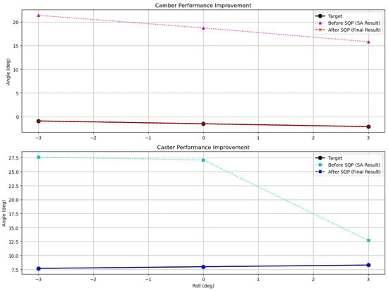
Figure 3. Camber and caster performance improvement achieved by the proposed hybrid QUBO–SQP framework. The dotted magenta and cyan lines denote the Stage 1 Simulated Annealing (SA) results obtained from the QUBO-based feasibility search, using first-order polynomial approximations of the nonlinear kinematic constraints. The dashed red and blue lines indicate the refined Stage 2 SQP results, computed under full-precision nonlinear equations. The solid black lines represent the target camber and caster curves.

The dashed curves (‘After SQP’) correspond to the refined geometry obtained after Stage 2, where the Sequential Quadratic Programming (SQP) optimizer operates on the full-precision nonlinear constraint model defined in Equations (11) and (12). The nearly perfect overlap of the dashed and solid curves confirms that SQP successfully corrected the approximation errors from Stage 1 and achieved complete convergence of both camber and caster to their target profiles.

This visualization thus provides a direct experimental validation of the mathematical modeling assumptions: the QUBO stage enforces feasibility under linearized constraints, while the SQP stage restores the full nonlinear model accuracy within numerical tolerance.

Figure 4 shows the optimization path achieved by the advanced QUBO-SQP hybrid algorithm. The magenta diamond represents the initial solution obtained from the Simulated Annealing (SA) stage, while the green cross denotes the final solution refined by the Sequential Quadratic Programming (SQP) stage. The plotted trajectory demonstrates how the hybrid framework progressively minimizes both camber and caster squared errors. This convergence highlights the complementary roles of SA in exploring the solution space and SQP in performing fine-grained local optimization, ultimately yielding an improved and balanced suspension design.

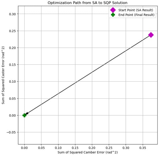
Figure 4. Optimization trajectory from the Simulated Annealing (SA) starting point to the Sequential Quadratic Programming (SQP) final solution in the proposed QUBO-SQP hybrid framework. The path illustrates the reduction in both camber and caster squared errors, converging to a balanced and optimal suspension configuration.

To quantify the precision of this final match, Figure 5 plots the absolute error between the final optimized curves and the targets on a logarithmic scale.

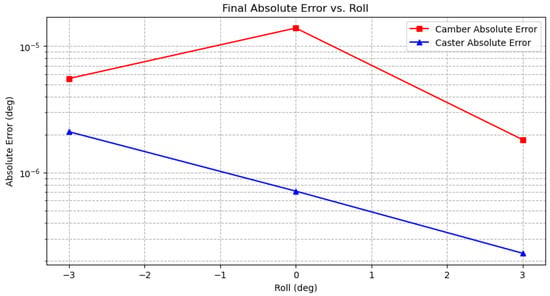
Figure 5. Final absolute error between the optimized and target curves. The logarithmic scale shows errors are on the order of ${10}^{-5}$ to ${10}^{-6}$ degrees, confirming a near-perfect convergence.

The final errors are exceptionally low, confirming that the solution is not just visually accurate but mathematically precise to the limits of numerical tolerance.

4.5. Comparison with State-of-the-Art Methods

To assess the benefits of the proposed hybrid QUBO–SQP framework, we compared it against three representative local improvement strategies initialized from the same QUBO-based design: Genetic Algorithms (QUBO–GA), Particle Swarm Optimization (QUBO–PSO), and gradient-based optimization (QUBO–GD). Table 4 reports the feasibility norm, camber and caster RMSE, and CPU time.

Table 4. Comparison with state-of-the-art optimization methods.

Method	Feasibility Norm	Camber RMSE (°)	Caster RMSE (°)	CPU Time (s)
QUBO–SQP (Proposed)	$3.433\times {10}^{-11}$	$8.010\times {10}^{-4}$	$2.129\times {10}^{-3}$	$1.4910$
QUBO–GA	$0.4897$	$20.2265$	$19.2383$	$0.7543$
QUBO–PSO	$0.3580$	$20.1906$	$19.5748$	$0.7664$
QUBO–GD	$1.094\times {10}^{-3}$	$8.9895$	$5.6293$	$13.4704$

QUBO–SQP consistently achieves near-perfect feasibility, with constraint norms on the order of ${10}^{-11}$, whereas QUBO–GD, QUBO–GA, and QUBO–PSO exhibit residuals of ${10}^{-3}$, ${10}^{-1}$, and ${10}^{-1}$, respectively. In terms of kinematic tracking, QUBO–SQP attains camber and caster RMSE below 0.003°, while all competing methods remain in the 6–20° range. Thus, the proposed framework improves both feasibility and tracking accuracy by several orders of magnitude compared to GA, PSO, and gradient-based baselines.

This superior accuracy is obtained at modest computational cost: QUBO–SQP requires ≈ 1.5 s per run, only slightly more than QUBO–GA and QUBO–PSO (≈0.75 s), and significantly less than QUBO–GD (≈13.5 s). Overall, the hybrid QUBO–SQP scheme provides the most favorable trade-off between feasibility robustness, convergence precision, and computational efficiency.

4.6. Discussion of the Hybrid Approach

The collective results synthesize into a powerful validation of our hybrid approach. The QUBO-SA stage successfully acted as an intelligent guess generator. By focusing solely on the difficult, nonlinear constraint satisfaction task, it provided the SQP stage with a starting point that was already physically valid. This prevented the SQP optimizer from getting trapped in nearby, but ultimately infeasible, regions of the design space. Unlike conventional hybrid heuristics, the QUBO–SQP architecture separates feasibility enforcement and precision optimization into distinct computational domains. The QUBO stage transforms constraint satisfaction into a binary energy minimization task, while SQP refines within the continuous constraint manifold. This architectural decoupling allows each stage to operate at maximal efficiency and avoids redundancy typical of heuristic–gradient hybrids.

The proposed QUBO–SQP formulation, defined by the objective function in Equation (10), is mathematically agnostic to the choice of target camber and caster trajectories. Because the targets enter the cost function parametrically, the optimization structure and solver configuration remain identical for any new desired functions. This property ensures that the framework is inherently adaptive to varying kinematic requirements without the need for reparameterization or additional case-specific studies. The effectiveness of this two-stage process can be visualized as a path in the objective space, as shown in Figure 6. The optimization began at the Start Point, which represents the high camber and caster error of the SA solution. The SQP algorithm then efficiently traversed the solution space, as indicated by the arrow, to arrive at the End Point, which lies at the origin of the plot, representing zero error.

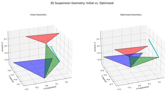
Figure 6. Visualization of the optimization process in the 3D objective space. The figure compares the initial and optimized suspension geometries. The red, green, and blue surfaces represent the upper control arm (UCA), lower control arm (LCA), and chassis plane, respectively, while the cyan line indicates the tie-rod connection. The framework moved the solution from a configuration with higher geometric error (Initial Geometry) to one with near-zero error (Optimized Geometry).

The underlying structure of the QUBO problem itself is revealed in the sparsity plot of its matrix Figure 7. The dense clusters of couplings represent the strong inter-dependencies between the binary variables that define a single geometric vector or angle. The sparser, off-diagonal elements represent the weaker but critical couplings between different physical components of the suspension. This visualization confirms that the problem is highly coupled and non-trivial, justifying the use of a powerful global search technique like SA.

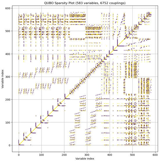
Figure 7. Sparsity plot of the $583\times 583$ QUBO matrix, visualizing the couplings between binary variables. The yellow and purple points represent positive and negative coupling coefficients, respectively. This plot highlights the structured sparsity of the optimization problem.

This study has limitations that present avenues for future research. The use of a first-order Taylor approximation in Stage 1 is effective but introduces inaccuracies that the SQP stage must correct. Exploring higher-order polynomial approximations could yield an even more accurate initial guess. Furthermore, the number of binary bits used for discretizations was kept low to ensure tractability on classical hardware. Scaling this approach to higher-resolution designs would benefit greatly from the use of hardware quantum annealers, which are purpose-built to solve such QUBO problems more efficiently. Finally, the framework could be extended to include more complex objectives, such as minimizing bump steer or managing forces within suspension components. Moreover, it is important to acknowledge that the assumption of separable feasibility and performance optimization central to the QUBO–SQP framework holds primarily for systems where constraint satisfaction and performance objectives are moderately coupled. In highly entangled mechanical systems, where geometric feasibility directly influences the performance landscape, this decoupling may introduce inaccuracies or limit convergence robustness. In such cases, the framework could be extended with higher-order constraint models or iterative coupling between QUBO and SQP stages to maintain fidelity. This consideration delineates the current scope of validity and outlines an avenue for future refinement of the hybrid approach.

5. Conclusions

This study presented a two-stage hybrid optimization framework for the high-dimensional, nonlinearly constrained geometry of a 3D double-wishbone suspension system. The proposed QUBO–SQP approach integrates a quantum-inspired Simulated Annealer (SA) for global feasibility search with a Sequential Quadratic Programming (SQP) algorithm for high-precision refinement. The framework achieved near-perfect convergence to the desired camber and caster targets, with a final objective value on the order of ${10}^{-14}$, demonstrating the effectiveness of decoupling feasibility enforcement from performance refinement.

The results confirm that the QUBO–SQP architecture successfully combines the global exploratory capability of quantum-inspired annealing with the precision of classical gradient-based optimization. Beyond suspension geometry, this methodology establishes a generalizable computational paradigm for complex engineering design problems characterized by nonlinear, high-dimensional constraint landscapes spanning domains such as robotics, aerospace mechanisms, and structural optimization.

Future work will extend this framework using variational quantum algorithms (VQAs) and hardware-based quantum annealing on D-Wave systems to achieve higher-resolution discretizations and further reduce computational cost. This line of research continues in our recent work [18], which experimentally integrates D-Wave quantum annealing with classical SLSQP refinement, demonstrating the feasibility of end-to-end hybrid quantum–classical suspension optimization.

Appendix A.1. Nominal Hard Point Data

$$\begin{array}{cc}\hfill {UCA}_{\mathrm{in}\_\mathrm{f}}& =[-0.080,-0.450,0.180]\hfill \\ \hfill {UCA}_{\mathrm{in}\_\mathrm{r}}& =[0.251,-0.490,0.185]\hfill \\ \hfill {UCA}_{\mathrm{out}}& =[0.041,-0.675,0.180]\hfill \\ \hfill {LCA}_{\mathrm{in}\_\mathrm{f}}& =[-0.199,-0.400,-0.195]\hfill \\ \hfill {LCA}_{\mathrm{in}\_\mathrm{r}}& =[0.201,-0.450,-0.190]\hfill \\ \hfill {LCA}_{\mathrm{out}}& =[0.001,-0.750,-0.245]\hfill \\ \hfill {TR}_{\mathrm{in}}& =[0.201,-0.400,-0.045]\hfill \\ \hfill {TR}_{\mathrm{out}}& =[0.151,-0.750,-0.045]\hfill \end{array}$$

Appendix A.2. Derivation of Optimization Vectors

The ten 3D vectors ($x\in R^{30}$) that constitute the geometric portion of our design variable vector are derived as follows:

• $o_{UB}$ (UCA Front-Inner Pivot): Set directly from the global coordinates of the front UCA chassis pivot.

  $$o_{UB}={UCA}_{\mathrm{in}\_\mathrm{f}}$$

  (A1)
• $o_{LB}$ (LCA Front-Inner Pivot): Set directly from the global coordinates of the front LCA chassis pivot.

  $$o_{LB}={LCA}_{\mathrm{in}\_\mathrm{f}}$$

  (A2)
• $o_{SB}$ (TR Inner Pivot): Set directly from the global coordinates of the Tie Rod inner pivot.

  $$o_{SB}={TR}_{\mathrm{in}}$$

  (A3)
• $p_{\mathrm{RearU}}$ (UCA Rear Pivot Vector): The vector from the front to the rear UCA chassis pivot.

  $$p_{\mathrm{RearU}}={UCA}_{\mathrm{in}\_\mathrm{r}}-{UCA}_{\mathrm{in}\_\mathrm{f}}$$

  (A4)
• $p_{\mathrm{RearL}}$ (LCA Rear Pivot Vector): The vector from the front to the rear LCA chassis pivot.

  $$p_{\mathrm{RearL}}={LCA}_{\mathrm{in}\_\mathrm{r}}-{LCA}_{\mathrm{in}\_\mathrm{f}}$$

  (A5)
• $p_{1U}$ (UCA Outboard Vector, Local Frame): The vector from the UCA’s front-inner pivot to its outer ball joint. In the nominal state (zero rotation), this is defined in the global frame.

  $$p_{1U}={UCA}_{\mathrm{out}}-{UCA}_{\mathrm{in}\_\mathrm{f}}$$

  (A6)
• $o_{HL}$ (LCA Outboard Vector, Local Frame): The vector from the LCA’s front-inner pivot to its outer ball joint.

  $$o_{HL}={LCA}_{\mathrm{out}}-{LCA}_{\mathrm{in}\_\mathrm{f}}$$

  (A7)
• $p_{2S}$ (TR Outboard Vector, Local Frame): The vector from the TR’s inner pivot to its outer end.

  $$p_{2S}={TR}_{\mathrm{out}}-{TR}_{\mathrm{in}}$$

  (A8)
• $p_{1H}$ (Upright UCA Vector, Local Frame): The vector defining the location of the UCA ball joint relative to the LCA ball joint, representing the upper part of the upright.

  $$p_{1H}={UCA}_{\mathrm{out}}-{LCA}_{\mathrm{out}}$$

  (A9)
• $p_{2H}$ (Upright TR Vector, Local Frame): The vector defining the location of the TR ball joint relative to the LCA ball joint, representing the steering arm of the upright.

  $$p_{2H}={TR}_{\mathrm{out}}-{LCA}_{\mathrm{out}}$$

  (A10)

Appendix B.1. Total Binary Variables

The model consists of 10 geometric vectors (three coordinates each) and 3 angle vectors (three coordinates each) evaluated at three roll points. While not all are constrained, the initial definition includes

• Geometric Variables: $10\mathrm{vectors}\times 3\mathrm{coordinates}/\mathrm{vector}\times 1\mathrm{bit}/\mathrm{coordinate}=30$ binary variables.
• Angle Variables: $3\mathrm{components}\times 3\mathrm{angles}/\mathrm{component}\times 3\mathrm{roll}\mathrm{points}\times 1\mathrm{bit}/\mathrm{angle}=27$ binary variables.

The total number of unique binary variables after the compiler’s expansion and optimization was 583.

Appendix B.2. QUBO Matrix Couplings

The resulting Q matrix was sparse. Out of a possible 583 × 583 ≈ 340,000 potential couplings, the model contained 6752 non-zero quadratic couplings. This sparsity is typical of physics-based models where interactions are localized to specific components, and it is a key feature that allows solvers like Simulated Annealing to find solutions efficiently. The structure of this sparsity is visualized in Figure 7 in the main text.

References

- Arshad, M.W.; Lodi, S. Optimization of Double Wishbone Suspension: Evaluating the Performance of Classes of Algorithms. In Proceedings of the 2024 International Conference on Applied Mathematics & Computer Science (ICAMCS), Venice, Italy, 28–30 September 2024; IEEE: New York, NY, USA, 2024; pp. 156–161. [Google Scholar] [CrossRef]
- Singh, A.; Pawar, S.; Soundalkar, M.; Ali, M.A. Design Optimization of the Control Arms of a Double Wishbone Suspension System Using Topological Approach. Int. J. Sci. Res. Eng. Manag. 2024, 8, IJSREM31250. [Google Scholar] [CrossRef]
- Wagh, S.Y.; Nandi, E. Design and Analytical Calculations of Double Wishbone for Formula Student Race Car. Int. J. Eng. Res. Technol. 2020, 9, 1029–1033. [Google Scholar] [CrossRef]
- Niu, Z.; Liu, S.; Li, B.; Pan, Z.; Wang, R. Explicit Solution to the Nonlinear Geometry of Double Wishbone Suspension by Decoupling Steering and Wheel Jumping DOF. Proc. Inst. Mech. Eng. Part D J. Automob. Eng. 2025, 239, 1495–1504. [Google Scholar] [CrossRef]
- Zhang, L.; Liu, J.; Pan, F.; Wang, S.; Ge, X. Multi-objective optimization study of vehicle suspension based on minimum time handling and stability. Proc. IMechE Part D 2020, 234, 2355–2363. [Google Scholar] [CrossRef]
- Zhang, B.; Li, Z. Mathematical Modeling and Nonlinear Analysis of Stiffness of Double Wishbone Independent Suspension. J. Mech. Sci. Technol. 2021, 35, 5351–5357. [Google Scholar] [CrossRef]
- Ashtekar, V.; Bandyopadhyay, S. Forward Dynamics of the Double-Wishbone Suspension Mechanism Using the Embedded Lagrangian Formulation. In Mechanism and Machine Science: Select Proceedings of Asian MMS 2018; Springer: Singapore, 2020; pp. 843–859. [Google Scholar] [CrossRef]
- Upadhyay, P.; Deep, M.; Dwivedi, A.; Agarwal, A.; Bansal, P.; Sharma, P. Design and analysis of double wishbone suspension system. In Proceedings of the International Conference on Mechanical and Energy Technologies (ICMET 2019), Greater Noida, India, 7–8 November 2019; IOP Publishing: Bristol, UK, 2020; Volume 748, p. 012020. [Google Scholar] [CrossRef]
- Garg, S.; Dudeja, S.; Gupta, S.; Rastogi, V. Optimization of a Double Wishbone Suspension Geometry for Off-road Vehicles using Genetic Algorithm and Machine Learning. In Proceedings of the 2022 13th International Conference on Mechanical and Aerospace Engineering (ICMAE), Bratislava, Slovakia, 20–22 July 2022; IEEE: New York, NY, USA, 2022; pp. 472–477. [Google Scholar] [CrossRef]
- Zhang, S.; Gao, Y.; Gao, D.; Pan, T.; Yang, J. Serial Combinational Optimization Method for Double Wishbone Suspension’s Pseudo Damage Improvement. Struct. Multidiscip. Optim. 2023, 66, 122. [Google Scholar] [CrossRef]
- Kulkarni, V.; Jadhav, A.; Basker, P. Finite Element Analysis and Topology Optimization of Lower Arm of Double Wishbone Suspension Using RADIOSS and Optistruct. Int. J. Sci. Res. 2014, 3, 639–643. [Google Scholar]
- Raikar, D.; Metar, M.; Attal, H. Design and Static Stress Analysis of Double Wishbone Suspension. Int. J. Res. Appl. Sci. Eng. Technol. 2022, 10, 249–257. [Google Scholar] [CrossRef]
- Metar, M. Structural Analysis of Double-Wishbone Suspension System. Int. J. Res. Appl. Sci. Eng. Technol. 2021, 9, 1681–1685. [Google Scholar] [CrossRef]
- Kumar, G.A.; Manepalli, P.; Narendran, R. Design optimization of double wishbone suspension system for motorcycle. In Proceedings of the International Conference on Advances in Thermal Engineering and Applications (ICATEA 2021), Online, 19–20 March 2021; IOP Publishing: Bristol, UK, 2021; Volume 2054, p. 012024. [Google Scholar] [CrossRef]
- Bhandarkar, S.; Nagose, A.; Sharma, D.; Bhasme, V. Design and Modification of Double Wishbone Suspension System in an ATV. Int. Res. J. Eng. Technol. 2020, 7, 6082–6087. [Google Scholar]
- Varthanan, P.A.; Jayasuriya, N.; Gowtham, V. Modification and Simulation of Double Wishbone Front Suspension in Safari SUV. J. Crit. Rev. 2020, 7, 150–157. [Google Scholar] [CrossRef]
- Prabaharan, T.; Herbert Bejaxhin, A.B.; Periyaswamy, P.; Ramanan, N.; Ramkumar, K. Lower Wishbone Modeling and Analysis for Commercial Vehicle Independent Suspension System. J. Mines Met. Fuels 2022, 70, 1143–1148. [Google Scholar] [CrossRef]
- Arshad, M.W.; Lodi, S.; Liu, D.Q. A Hybrid Quantum-Classical Approach Using D-Wave and SLSQP for Double Wishbone Suspension System Optimization. In Proceedings of the 2025 IEEE Conference on Artificial Intelligence (CAI), Santa Clara, CA, USA; 2025; pp. 16–19. [Google Scholar] [CrossRef]
Disclaimer/Publisher’s Note: The statements, opinions and data contained in all publications are solely those of the individual author(s) and contributor(s) and not of MDPI and/or the editor(s). MDPI and/or the editor(s) disclaim responsibility for any injury to people or property resulting from any ideas, methods, instructions or products referred to in the content. |
© 2025 by the authors. Licensee MDPI, Basel, Switzerland. This article is an open access article distributed under the terms and conditions of the Creative Commons Attribution (CC BY) license (https://creativecommons.org/licenses/by/4.0/).