Revealing Encoded Images Using a Generative Adversarial Network

Abstract

In this work, we address a special challenge for a generative adversarial network, which is to reveal images encoded using dynamic S-boxes based on a cryptographically secure pseudo-random number generator. S-boxes are generated by the logistic function with two time series with delays, resulting in a robust coding. A conditional generative adversarial network (cGAN) designed for image translation is used. Experiments were performed on datasets where image intensity levels varied between 256, 128, 64, 32, and 16 while keeping the image size constant. The main findings can be summarized as follows: a cGAN can be trained to reveal images encoded by S-boxes; the quality of the translated images improves as the number of intensity levels decreases, with images with 16-intensity levels being the sharpest and sharpness decreasing as intensity levels increase; and in an experiment where the input and output images were reversed, cGAN was found to learn to encode images according to the S-boxes method. It was found that a double translation, consisting of first encoding a real image by the reverse experiment and then a second translation to reveal the encoded image, recovered the original image. The translated training and test images resulting from these experiments were evaluated using binary analysis and metrics derived from the confusion matrix.

1. Introduction

Generative neural networks are one of the pillars of machine learning and a major driver of AI advancement. A conditional generative adversarial network (cGAN) allows the generation of one image conditioned on another. The Pix2Pix cGAN is an implementation of a conditional generative adversarial network (cGAN) that allows image translation. Phillip Isola et al. [1] published a seminal paper establishing a general-purpose solution for image-to-image translation. Since the problem we address here is to reveal an encoded image, that is, to translate an encoded image into its corresponding real image, this problem is solved in this work by using conditional generative neural networks.

GANs are a type of deep learning model designed for generative tasks. They were introduced by Ian Goodfellow in 2004 [2] and have become a hot area of research in machine learning and artificial intelligence. GANs have two main components: (i) a generator, a network that generates new data instances from random noise or a latent vector and whose goal is to produce data that are indistinguishable from real data; and (ii) a discriminator, a neural network that evaluates the data generated by the generator, distinguishing between real data from the database and fake data generated by the generator model. The objective of the discriminator model is to correctly identify real data from the generated data. We find that cGANs are well suited to address our problem of revealing encoded images, as the input image that the generator and discriminator incorporate during the training process is the encoded image for both networks; the real image is the conditional image for the generator model.

Conditional GANs have diverse applications in several fields, particularly in computer vision, such as image-to-image translation, where they can transform images from one domain to another based on specific conditions. Among its most important applications are image manipulation and transformation, such as converting sketches into realistic images [3]; text-to-image synthesis to generate images from textual descriptions [4,5]; image-to-image translation, as in our case, where images from the encoded image domain are transformed into the real image domain [6]; applications in medical imaging for tasks such as image segmentation and high-resolution medical image generation [7]; and the generation of handwritten characters, such as Devanagari script [8]. However, it is also applied to image super-resolution, improving the quality of low-resolution images [9,10]. It is worth mentioning the StegoPix2Pix version, which has been adapted for steganography, which involves hiding secret data in images [11].

One line of work that led to important results was to vary the number of intensity levels (or radiometric resolution) in the processed images, keeping the image dimension (or spatial resolution) constant (256 × 256). The image bits per pixel ranged from 8, 6, 5, and 4, corresponding to 256-, 64-, 32-, and 16-intensity levels, respectively. The translated images, both those generated by the training dataset and the test images, were evaluated using binary analysis and metrics derived from the confusion matrix. The sharpness of the translated test images improved as the number of intensity levels decreased, while for the translated images from the training dataset, the difference was practically zero. This sharpening effect on the test images is discussed in terms of the U-Net architecture of the generator model.

The results obtained in the reverse experiment are also analyzed and discussed using the metrics derived from the confusion matrix. In this experiment, the input and output images are inverted such that the input image is the real image and the generated image is the encoded image. In this case, a double translation was performed and the original real image was recovered. From the reverse experiment, we found that the cGAN is capable of encoding real images by emulating dynamic S-box encoding, and also consistent in recovering the original real images through a second translation.

In a previous work [12], the Gaussian function technique was used to reveal encoded images. The procedure was successful, so it was also implemented to reveal encoded RGB images [13], which could also be revealed. However, this method requires selecting the Gaussian parameters by trial and error. We realized that it is necessary to implement a machine learning-based method to reveal these coded images in a more systematic way.

2. Materials and Methods

This section presents the method used to encode images by generating dynamic S-Boxes; the operation of the Pix2Pix conditional generative adversarial network is described in terms of the generator and discriminator models. The method used to generate images with intensity values of 16, 32, and 64 from original images with 256-intensity values is provided. The need to introduce a seed to generate random numbers in the coding process is explained to ensure experimental reproducibility. Information is also provided on the image training procedure, the setup of the experiments, including network parameters and hyperparameters, and the datasets used in the experiments.

Generation of Dynamical S-boxes.Encoding image method.

An image $m\times n$ is codified by m different substitution boxes (S-box), that is, an S-box for each row of an image [14]. Each S-box is generated by a pseudo-random series $z_0,z_1,z_2,\dots$, where $z_i\in {\mathbb{Z}}_0^{255}=\{0,1,2,\dots ,255\}$ is a segment of integer numbers from zero to 255. Note that the cardinality of ${\mathbb{Z}}_0^{255}$ is equal to the intensity levels of an image. However, the length of $z_i$ depends on the array that contains all the elements of ${\mathbb{Z}}_0^{255}$. The S-box is generated according to how the different values of ${\mathbb{Z}}_0^{255}$ appear. The 256-intensity levels of each pixel in an image are modified according to time series $z_i$. The chaotic time series are generated with the extended logistic map given by

$$x_{n+1}=f\left(x_n\right)=\lambda x_n(2^k-x_n); k,n\in {\mathbb{N}}_0,$$

(1)

where ${\mathbb{N}}_0$ is the set of natural numbers and zero.

Theorem 1.

The extended logistic map given by (1) presents an invariant set $I=[0,2^k]$ for $\lambda ={\displaystyle \frac{1}{2^{k-2}}}$.

Proof. 

If the extended logistic map is continuous and $f^{\prime }\left(x_n\right)=\lambda (2^k-2x_n)$, then a maximum value occurs at $(2^{k-1},2^k)$. $f^{\prime }\left(x\right)>0$ for $x\in [0,2^{k-1})$, f is a monotone increasing function, and $f^{\prime }\left(x\right)<0$ for $x\in (2^{k-1},2^k]$, making f a monotone decreasing function. For the two intervals $I_1=[0,2^{k-1}]$ and $I_2=[2^{k-1},2^k]$, we have $I=I_1\cup I_2$ and

$$f\left(I_1\right)=I \mathrm{and} f\left(I_2\right)=I.$$

Therefore, $I=[0,2^k]$ is an invariant set of f. □

Mathematically, the parameter $\lambda$ could be negative, and thus the next proposition is given.

Theorem 2.

The extended logistic map given by (1) presents an invariant set $I=[-2^{k-1},3·2^{k-1}]$ for $\lambda =-{\displaystyle \frac{1}{2^{k-1}}}$.

Proof. 

We have $f^{\prime }\left(x_n\right)=\lambda (2^k-2x_n)$, and now a minimum value occurs at $(2^{k-1},-2^{k-1})$. If $f^{\prime }\left(x\right)<0$ for $x\in [-2^{k-1},2^{k-1})$, then f is a monotone decreasing function, and if $f^{\prime }\left(x\right)>0$ for $x\in (2^{k-1},3·2^{k-1}]$, then f is a monotone increasing function. For the two intervals $I_1=[-2^{k-1},2^{k-1}]$ and $I_2=[2^{k-1},3·2^{k-1}]$, we have $I=I_1\cup I_2$ and

$$f\left(I_1\right)=I \mathrm{and} f\left(I_2\right)=I.$$

Therefore, $I=[-2^{k-1},3·2^{k-1}]$ is an invariant set of f. □

For $k=8$, we have two values for parameter $\lambda$ according to Theorems 1 and 2, $\lambda ={\displaystyle \frac{1}{2^6}}$ and $\lambda =-{\displaystyle \frac{1}{2^7}}$, respectively. Then, for these values of the parameter $\lambda$, we generate two series of chaotic times, $x_i$ and $y_i$ for $\lambda =-1/2^7$ and $1/2^6$, respectively.

Figure 1 shows the U-shape distributions of the time series of the extended logistic map given by Equation (1) for the parameter $\lambda$: (a) ${\displaystyle \frac{1}{2^6}}$ and (b) $-{\displaystyle \frac{1}{2^7}}$. The goal is to generate time series with a uniform distribution. To achieve this goal, in the same spirit as [15], we generate two chaotic time series by using the extended logistic map (1):

$$x_{n-10}^{\prime }=x_n+x_{n-5}+x_{n-10} mod 2^8,$$

(2)

$$y_{n-10}^{\prime }=y_n+x_{n-6}+x_{n-10} mod 2^8,$$

(3)

with $n=10,11,\dots$.

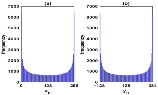
Figure 1. U-shape distributions of the time series of the extended logistic map given by (1) for the parameter $\lambda$: (a) ${\displaystyle \frac{1}{2^6}}$ and (b) $-{\displaystyle \frac{1}{2^7}}$.

Figure 2 shows the distributions of the time series: (a) $x_n^{\prime }$ and (b) $y_n^{\prime }$, by considering lags as they are determined by Equations (2) and (3).

$$z_n=x_n^{\prime }+y_n^{\prime } mod 2^8.$$

(4)

Figure 2. Distributions of the time series $x_n^{\prime }$ and $y_n^{\prime }$ considering lags as is determined by Equations (2) and (3).

Figure 3 shows the distributions of the time series $z_n$ by considering Equation (4).

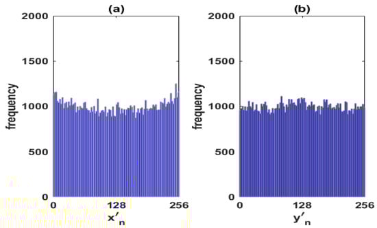
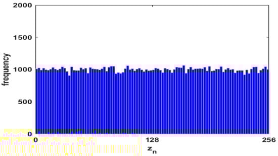
Figure 3. Uniform distributions of the time series $z_n$ given by (4).

Remark 1.

The logistic map $L_{\mu }:[0,1]\to [0,1]$, given by $L\left(x\right)=\mu x(1-x)$, for $\mu \in (0,4]$, shows chaotic behavior for values of the parameter μ in a small interval close to 4. Similarly, the extended logistic map for a given k resembles the chaotic behavior of the logistic map for values of the λ parameter in a small interval close to ${\displaystyle \frac{1}{2^{k-2}}}$. This gives us the opportunity to choose other values of the λ parameter and guarantee the chaotic behavior generated by the extended logistic map. However, parameter values close to ${\displaystyle \frac{1}{2^{k-2}}}$ do not guarantee the invariant set $[0,2^k]$ and generate a different invariant set $[a,b]$ that could be used to generate dynamical S-boxes.

Remark 2.

Theorems 1 and 2 are given for arbitrary k and values larger than $k=8$ may be used because Equations (2) and (3) consider the modulo operation. The modulo operation $\left(mod{2}^8\right)$ generates the required values to the encoding mechanism.

Remark 3.

The invariance properties of the extended logistic map ensure that any arbitrary seed in the invariant set has a bounded chaotic orbit useful for generating dynamical S-boxes.

The Conditional Generative Adversarial Networks—Pix2Pix. To illustrate the general procedure followed in the experiments carried out in this work, a general flowchart (Figure 4) is presented, showing the encoding of the datasets, the experiments carried out with cGANs, and the evaluation of the results using binary analysis. The description of the operation of a cGAN is done in terms of the generator and discriminator models and is illustrated in Figure 5 for the case addressed in this work. The operation is focused on the Pix2Pix cGAN used in this work.

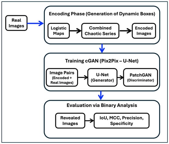
Figure 4. General flowchart of the experiments. The figure illustrates the procedure followed in the experiments performed in this work. The diagram shows the encoding of the datasets, the experiments performed with cGANs, and the evaluation of the results using binary analysis.

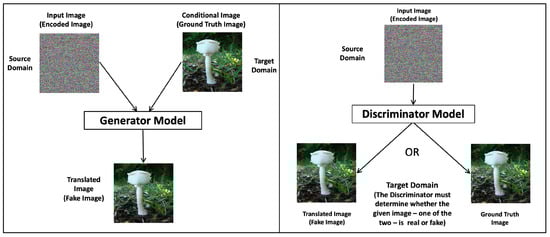
Figure 5. Generator and discriminator models. Left: Generator model. The figure shows the input and output images of the generator model. The input image from the source domain is the encoded image and the output image is the translated image (fake image). The image was generated conditioned on the real image of the target domain. Right: Discriminator model. The discriminator model uses the encoded image as input and an image from the target domain, either the generated (fake) image or the real image. The discriminator model outputs the probability that the target domain image is a translation of the encoded image.

GANs have two models: the generator model and the discriminator model. The discriminator model is trained to classify images as real (from the real image dataset) or fake (generated). The generator model is trained to fool the discriminator model. Conditional GANs learn a conditional generative model. This makes cGANs suitable for image-to-image translations, where an input image is conditional (the encoded image is conditioned by the real image, in our case) and generates the corresponding output image, the revealed image (Ref. [1]).

In our experiments, we provide the discriminator model with an encoded image as the input image and an image from the target domain, either the real or the generated image, and must determine whether the image is real or fake (Figure 5). The generator model is trained with a dual purpose: to fool the discriminator model and to minimize the loss between the generated image and the expected target image. In our experiments, Pix2Pix cGAN is trained with a dataset of encoded images as input images and the dataset of corresponding real images, which are the output target images. The datasets are integrated in such a way that each encoded image is paired with its corresponding real image. The generator model has an encoded image of the source domain as input and a generated image of the target domain as output. The generating model architecture includes a U-Net, as illustrated in Figure 25.

On the other hand, the discriminator model takes an encoded image from the source domain and an image from the target domain, which could be the actual image from the dataset or the generated image. The discriminator model outputs the probability that the target domain image is a translation of the encoded image.

P. Isola et al. [1] designed an architecture for the discriminator model called PatchGAN that penalizes the image structure at the patch scale. The discriminator tries to classify whether each patch of N × N pixels (in our case, 70 × 70 pixels) in an image is real or fake. This discriminator runs convolutionally over the image, averaging all responses to obtain the final output of the discriminator model.

Generation of Datasets with 64-, 32-, and 16-Intensity Levels. To reduce the number of intensity levels from 256 (for the original images) to 64, 32, or 16 (for the new datasets), a subset of intensity levels was generated for each case. The new sets of intensity values are in the range [0, 255]. For example, to generate a dataset of 16–intensity levels from images with 256 intensities, we select the new set of 16-intensity levels in the range [0, 255]. The new intensity levels could be the set [0, 17, 34, 51, …, 221, 238, 255]. The original intensity levels are assigned to these new levels by an algorithm that assigns the closest new intensity value to the original values. Therefore, the original intensity values [11, 12, …, 16, 17, 18, …, 25] will be assigned to the intensity value 17, while the intensity values from 26 to 42 will be assigned to the new value 34, and so on. To facilitate image processing, the quantification of the pixel intensity of the dataset was modified but always keeping the image dimension or space resolution constant at 256 × 256, i.e., the pixel density was kept constant across all datasets. This allowed the pixel density to be maintained in the datasets while decreasing the quantization of pixel intensities. This artifact of reducing the number of bits per pixel was used to make image processing operations simpler and faster, due to the reduction in intensity levels. Figure 6 shows the same image, but with a different number of intensity levels (or radiometric resolution) varying between 256, 64, 32, and 16. It is difficult to notice differences between these images despite their different intensity levels. The human eye can only discriminate differences in the tones of the images from 16 intensity levels, making it difficult to distinguish the differences between the images in Figure 6.

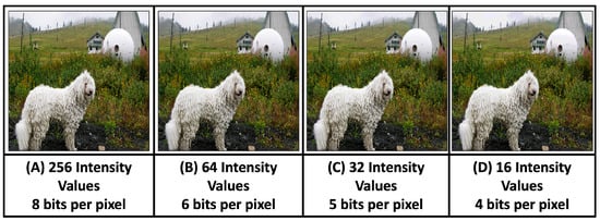
Figure 6. The figure shows the same image with 256- (A), 64- (B), 32- (C), and 16- (D) intensity levels. The image with 256-intensity levels was used to generate the other images, applying the algorithm designed for this purpose. Training and test datasets with 64-, 32-, and 16-intensity levels were created to conduct experiments to reveal images encoded using the Pix2Pix network. In each dataset, the encoded images also had the same intensity levels as the real images.

Using a seed to generate S-boxes. Image encoding. The generation of S-boxes using a seed was done by applying a different S-box to each row of the image matrix, making the encoding rule different for each row of the image matrix, which makes it a robust encoding. The S-boxes’ generation described above requires a pair of random numbers to be entered into Equations (2) and (3) to calculate the two time series. Using a seed to generate the random numbers required for the time series is critical to ensuring that the experiments are reproducible. Experimental reproducibility would be impossible if the random numbers in Equations (2) and (3) were generated without a seed, since the encoding of the same image would be different each time it is encoded because the encoding algorithm will generate a different pair of random numbers. This will cause the algorithm to generate different S-boxes and therefore produce a different encoded image, making reproducibility of the experiment impossible. Therefore, a seed was used in the encoding algorithm to generate the random numbers.

Image processing, setting up experiments and training datasets. The training dataset contained 1505 images, and 100 images were used in the test dataset. For each experiment, 200 epochs were run with a batch number of 1; that is, each image was processed 200 times, and 301,000 iterations were performed with the 1505 images from the training dataset. The best results occurred between epochs 100 and 200, for each of the datasets of 256-, 64-, 3-, and 16-intensity levels. It is important to note that the generated images can have up to 256 intensity levels, although the input ground-truth or encoded training images had 64 or fewer intensity values. This always happens, regardless of the number of intensity values in the input datasets, as the translated images always attempt to recover 256-intensity levels. The Pix2Pix cGAN hyperparameters were kept constant throughout all experiments. For the discriminator model, the activation function was a sigmoid. The loss function was binary cross-entropy and the optimization function used was Adam with a learning rate of 0.0002 and a beta value of 0.5. For the generator model, the activation function was a ReLU and the model GAN had Adam optimization with a learning rate of 0.0002 and beta 0.5. The loss function was binary cross-entropy.

The experiments were carried out using Pix2Pix cGAN. The training and test datasets were obtained from the ImageNet dataset (Large Scale Visual Recognition Challenge 2017—ILSVRC2017 [16]. The algorithm by Philip Isola et al. [1] and the corresponding code for Pix2Pix cGAN developed by Jason Brownlee [17] were used to translate the encoded images.

Computing infrastructure. The experiments were carried out on the Thubat Kaal Cluster at the IPICYT Supercomputing Center. This high-performance Bull computer has a theoretical processing power of 224.5 teraflops and 69 computing nodes. It features Intel Xeon Skylake 6130 16c processors clocked at 2.1 to 3.7 GHz and 192 GB of RAM.

3. Results

This section contains three categories of results: the results with training datasets, the results with test datasets, and the results of the inverse experiment along with the images obtained by double translation. In each case, except for the reverse experiment, results are presented with 256-, 64-, 32-, and 16-intensity levels. In addition, RGB image translation analyses based on intensity histograms are performed. These results are discussed briefly here in a qualitative manner, leaving the quantitative analysis based on image metric scores for the Section 4.

3.1. Training Experiments with the 256-, 64-, 32-, and 16-Intensity Levels Datasets

Figure 7 shows a set of 12 real images used in the training experiments. These images belong to the training dataset of 256-intensity levels. The corresponding encoded images are presented below each real image. Encoding completely hides the features of real images.

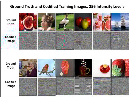
Figure 7. Images with 256-intensity levels. A set of real images from the training dataset is shown along with their corresponding encoded images. Encoding completely hides the ground truth features of images.

After 150–160 Epochs (or 225,750–240,800 iterations), the model generated the images shown in Figure 8. As is well known, GANs do not have an objective way to assess training progress in terms of the quality of the generated images. Therefore, as usual, we saved images periodically during the model training process. We qualitatively evaluated the generated images and, based on our criteria, selected the model that generated the best images. However, we also quantitatively evaluated the quality of the generated images. To do so, we developed a binary analysis and, based on the metrics derived from the confusion matrix, evaluated the quality of the generated images. The results are presented in the Results section. For training experiments, the quality of the translated images is generally high.

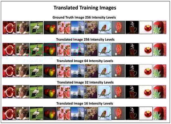
Figure 8. Translated training images. Experiments with training datasets of 256, 64, 32, and 16 intensity levels (8, 6, 5, and 4 bits). The figure shows the ground truth images and their corresponding translated images for each dataset. The translated images were generated with models obtained after 150–160 training epochs (or 225,750–240,800 iterations). The training dataset contained 1505 images. For training experiments, the quality of the translated images is generally high. The quantitative evaluation of the translated images is presented in Section 4.

Analysis of Training Images Based on Intensity Histograms

One way to assess the quality of translated images is through their intensity histograms. Indeed, a comparative analysis of the intensity histograms of the translated images versus the ground truth images allows us to visualize, in each RGB channel, the cGAN’s ability to reproduce the ground truth images. Figure 9 shows the intensity histograms of the translated image with 64-intensity levels (left) and the ground truth image of 256-intensity levels (right); the images from which the histograms were obtained are also shown. The images and histograms show a high degree of agreement. Note that the originally translated image with 64-intensity levels recovers the 256-intensity levels.

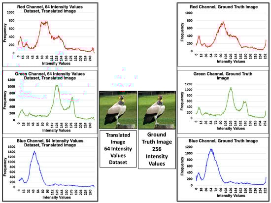
Figure 9. Histograms of the translated image with 64-intensity values and of the ground truth image with 25-intensity levels from the training dataset. Histograms of the three RGB channels of both images are shown. The intensity frequency values of the translated images (left) match those of the ground truth image (right) for all three channels. The translated image, originally from the 64 intensity dataset, recovered all 256 intensity values.

3.2. Test Experiments with the 256, 64, 32, and 16-Intensity Levels Datasets

The translated images obtained in the experiments with the four test datasets (16-, 32-, 64-, and 256-intensity values) are presented. Translating training images assesses cGAN’s ability to learn a specific task, in this case, revealing encoded images, a complex task in itself. Once the training process is complete, and if all goes well, the trained model is expected to be able to translate, in addition to the 1505 images in the training dataset, any other unknown encoded image that was not in the training dataset, which is a more complex task. In this case, we are considering an image encoded according to the process described in the Introduction. Therefore, revealing an encrypted image from the test dataset is an important evaluation for the neural network in which its prediction ability is tested, and the result is important for the research area of cryptanalysis. The translated images of the four test datasets having different intensity values are presented. For all datasets, the same set of 12 translated test images is shown to facilitate comparison between the experiments performed. The quantitative analysis of the translated test images is presented in Section 4.

Figure 10 shows the revealed images obtained from the translation of the encoded test images from the experiments with all test datasets. As can be seen, the quality of the translated images improves as the number of intensity values decreases. The best results correspond to test images with 16 intensity values, whereas images with the lowest definition are those with the highest number of intensity values.

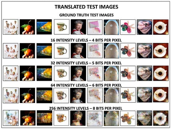
Figure 10. Translated test images obtained using the models generated in the experiments with the datasets of 16-, 32-, 64-, and 256-intensity values. The sharpness of the images depends on the number of intensity values in the dataset, which improves as the number of intensity values decreases. This result is different from that obtained with the training images, where the definition of the images was practically constant for all intensity datasets. An interpretation of this effect will be given in Section 4.

It is interesting to note that for the test images, the sharpness of the images depends on the number of intensity values in the dataset, while for the training images, the sharpness of the images was quite independent of the number of intensity values of the dataset and was quite consistent. An interpretation of this effect will be given in Section 4 based on the processing performed by the U-Net.

In Figure 11, we highlight the results for the 16-intensity dataset. The revealed images have a very similar quality to that obtained with the training datasets. Figure 10 and Figure 11 indicate that there is a mechanism in the Pix2Pix cGAN’s image processing that improves the translation of encoded images as the number of intensity values decreases. We will return to this point later in Section 4.

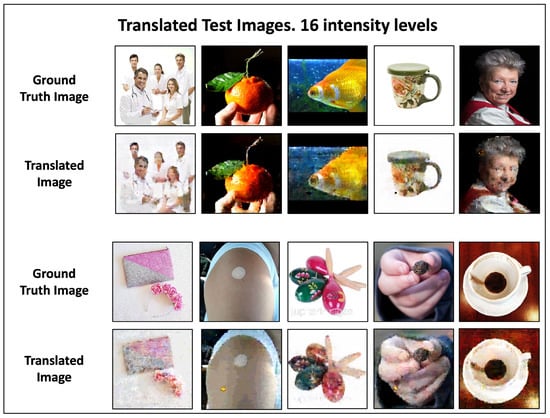
Figure 11. Translated test images generated by the 16-intensity dataset. The translated images from the 16-intensity test dataset are highlighted. These are the sharpest translated images from the test datasets. The quantitative analysis carried out in Section 4 confirms this assertion.

3.3. Reverse Experiment

Performing this experiment is interesting because, in this process, the GAN network is expected to encode or encrypt the input image. In the reverse experiment, the generator model uses the real image as input; the conditional image is the encoded image from the target domain; and the translated encoded image (fake image) is the image generated by the generator model. The discriminator model also has the real image as input image and must select one of the encoded images in the target domain, the translated encoded image or the S-Boxes encoded image.

The reverse experiment leads to the search for an answer to the question of the ability of the neural network to emulate the coding of real images according to the procedure used in this work: Is the encoding performed by the neural network consistent with the encoding performed by S-boxes as described in Section 1? Coding and its consistency can be assessed by translating the encoded image generated in the reverse experiment a second time. This second translation is performed using the model generated in the forward experiment, in which the encoded image is revealed. A double translation is necessary, since the encoded image was translated by the reverse experiment, and to reveal the original real image, a second translation is necessary. If the result of this double translation allows the original real image to be recovered, it will mean that the encoding performed by the Pix2Pix network successfully emulated the encoding performed by the S-boxes.

Double translation in the reverse experiment was performed on images from the training and test datasets. The quality of the training images obtained through double translation is good considering the double process performed. Figure 12 shows doubly translated images, ground truth images, as well as the encoded images generated by this experiment and the ground truth images encoded by S-boxes that were inputted into the cGAN.

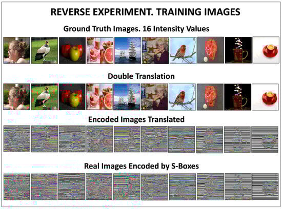
Figure 12. Reverse experiment. Doubly translated images from the training dataset. A set of 10 images from the training dataset is shown. The first row shows the ground truth images of 16-intensity values. The images generated by the double translation are shown in the second row, while the third and fourth rows contain the translated encoded images obtained from the inverse experiment and the images encoded from the ground truth images using S-boxes, respectively.

The result of applying double translation to the images of the test dataset is shown in Figure 13. The first row shows the ground truth images and the second row shows the doubly translated images. The third and fourth rows contain encoded images; the translated encoded images appear in the third row and the ground truth images encoded by S-boxes in the fourth row.

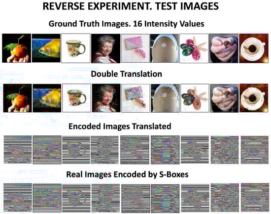
Figure 13. Reverse experiment. A set of images from the test dataset is shown. The first row shows the ground truth images. The double translation of the test dataset images is shown in the second row. The third row contains the encoded images translated in the reverse experiment, and the fourth row shows the ground truth images encoded by S-Boxes.

Analysis of the Reverse Experiment Based on Intensity Histograms

Histograms (Figure 14) show the intensity values of the three RGB channels of the encoded images shown in Figure 15. The left column shows the intensity histograms of the channels of the translated training image obtained in the reverse experiment. The second column shows the three channels of the actual 8 bpp-encoded images. The right column presents the channels of the 4 bpp-encoded image, which, in this experiment, is the conditional image of the generator model. In the first and second columns, it can be seen that the histograms of the translated encoded image with 16-intensity values and those of the real image encoded with 256-intensity values present a homogeneous frequency distribution in the range [0, 255], as expected from a well-encoded image. It should be noted that the translated encoded image was processed having as input and conditional images images with 16-intensity values and that, after being processed, it acquired tones in the entire intensity range [0, 255].

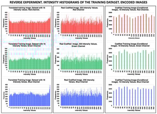
Figure 14. Intensity histograms obtained from an image of the training dataset processed in the inverse experiment. Since the images generated in this experiment are encoded images, the first column contains the intensity histograms of the three channels of the translated trained image (encoded image). The second column shows the histograms of the 256-intensity values encoded image, and the third shows the histograms of the encoded training image. The latter histograms show the 16-intensity values of the encoded image. As expected, the intensity histograms of the encoded images show a homogeneous distribution across the entire intensity range [0, 255].

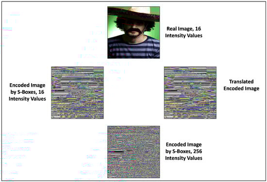
Figure 15. Images used to generate the histograms in Figure 14. The three encoded images belong to the training dataset. For the inverse experiment, the input image is the real image (top), the translated image encoded by the cGAN and the one encoded by S-Boxes are in the middle. Finally, the 256-intensity image, also encoded by S-Boxes, is shown as a reference at the bottom.

To evaluate the ability of the Pix2Pix neural network to recover the original real images after two translations, the intensity histograms of the test images generated by double translation were analyzed. These were compared with the intensity histograms of the real images translated once, as well as with the histograms of the real images with 256-intensity values. Figure 16 shows the three-channel RGB histograms of the translated test images and the histograms of the 256-intensity ground truth image. The intensity frequency patterns of the histograms exhibit a high degree of coincidence. In this reverse experiment, the input real image and the conditional encoded image (target domain) have 4 bpp (16-intensity values). However, the translated encoded image was generated by the neural network with 256-intensity values, as can be seen in the histograms in Figure 14.

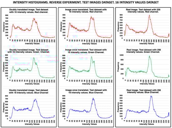
Figure 16. Intensity histograms of the inverse experiment for the three RGB channels. The histograms correspond to images processed originally with 16-intensity values from the test dataset. Histograms of doubly translated images are presented in the first column (see images in Figure 13). The second column shows the histograms of a translated image, and the third shows the histograms of the real image with 256-intensity values. The intensity histogram patterns of the translated images are highly consistent with those of the real image.

4. Discussion

This section presents and discusses the quantitative results relating to the quality of the translated images. The binary analysis method selected to evaluate the revealed images is described, and the confusion matrix metrics are derived. Given the FP=FN identity that occurs for the binarized images that were used, its effect on the applied metrics is analyzed. In addition, the results of the quality of the translated images are presented in terms of the evaluation metrics. In addition, the results of the translated image quality are presented in terms of the evaluation metrics. These include the training and test datasets, as well as the reverse experiment, taking into account double translation. Finally, an analysis of the complexity of the method is presented, the limitations of this approach are mentioned, and a brief account of the possible applications is given.

cGANs evaluation. Unlike other deep learning neural network models that are trained using a loss function until convergence is reached, this is not the case with cGANs. The cGAN generator and discriminator models are trained together to maintain an equilibrium. Therefore, there is no objective way to evaluate the progress of training or the quality of the model. A general problem with GANs is that there is no objective way to assess the quality of images generated during training. For this reason, it is common to periodically save some images generated during training and, based on a subjective human evaluation of the generated images, select the generator model that is considered the best. Many attempts have been made to establish an objective method for measuring the quality of generated images. However, virtually all focus on the ability of different GANs to translate images [18], rather than on measuring the quality of images generated from an encoded image, as is our case. For this reason, we have resorted to performing binary analysis and applying the metrics derived from the confusion matrix.

Binary Analysis. Confusion Matrix Elements. In order to objectively quantify the ability of the cGAN neural network to reveal real images from encoded images, a binary analysis was performed to compare the generated images with the real images. For this purpose, the images were segmented into four intervals of 64-intensity values each: [0, 63], [64, 127], [128, 191], [192, 255]. The images were binarized using an algorithm that works as follows: a segment of intensity values is selected, for example, [0, 63], and it is checked which elements of the image array are within the range of this segment. For those that are, the pixel position in the image array is assigned the value 1; otherwise, it is assigned 0. This process was performed for the four segments in each of the three RGB channels of the generated image and also for the real image. Once both image matrices (the ground truth and the translated image) were binarized, the elements of the confusion matrix were generated by comparing the elements of the matrix of the translated image with those of the ground truth image. The translated and ground truth images, once binarized, were analyzed using this procedure, testing, pixel by pixel, all possible combinations of this binary scheme to obtain the elements of the confusion matrix. There are only four possible combinations between the elements of the two binarized matrices of the images, which, expressed as pairs, are the following: [1, 1], [0, 0], [1, 0], and [0, 1]. The first pair [1, 1] means that, at the same pixel position in both image matrices, the intensity value was within the range of the processed segment in both the generated and real images. According to the confusion matrix, the names of the elements of the four possible combinations of these pairs are: True Positive (TP), True Negative (TN), False Positive (FP) and False Negative (FN), respectively.

The results obtained from a binary analysis of a generated and a real image are shown in Figure 17. Graph (A) illustrates the result of performing a binary analysis on a single image channel; the four segments are broken down and for each segment the elements of the confusion matrix TP, TN, FP, and FN are shown. On the right side, graph (B), the results for the three channels of an RGB image appear; each element of the confusion matrix is broken down by channel and by the total RGB image.

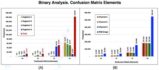
Figure 17. Binary analysis of a test image. Graph (A) shows the binary analysis of a single image channel and the elements of the Confusion Matrix (False Negative (FN), False Positive (FP), True Positive (TP) and True Negative (TN)) are broken down by segment. The binary analysis of the three channels of the RGB image, graph (B), shows the elements of the confusion matrix broken down by channel and the total RGB image. Notice that the FN values are equal to those of the FP for every channel and for the whole image. This equality has important consequences for the metrics.

Note that for each channel and for the entire RGB image, the number of false positives (FP) is always equal to the number of false negatives (FN). A consequence of the equality $FP=FN$ is that the following metrics are equivalent:

$$Precision (Positive Predictive Value, PPV) = Recall (True Positive Rate) = F1 Score,$$

(5)

$$Negative Predictive Value \left(NPV\right) = Specificity.$$

(6)

Furthermore, these metrics are also equivalent:

$$Informedness = Markedness = Mattews Correlation Coefficient \left(MCC\right).$$

(7)

All of these equivalences follow directly from the definitions of the metrics. For this reason, from now on we will only report the Precision, Specificity and MCC metrics. Additionally, we will also report the Intersection over Union (IoU) parameter, which is the fraction of True Positives and True Negatives with respect to the total:

$$IoU=(TP+TN)/(TP+TN+FP+FN),$$

(8)

The reason why false positives are always numerically equal to false negatives $(FP=FN)$ is due to the binary nature of image matrices. By analyzing the two binary matrices of the images, and considering the images as sets, it can be shown that the intersection is given by the sum of the True Positive and True Negative elements $(TP+TN)$. The elements that are not at the intersection of the two matrices are false positives (FP) and negatives (FN). Given the binary nature of the matrices and knowing that the elements FP and FN are not at the intersection as well as the definition of each of them, it can be shown that the number of False Positives is equal to that of False Negatives.

Evaluation Metrics. Focusing on our problem of quantitatively evaluating the quality of translated images, we applied the metrics Specificity (equal to Negative Predictive Value-NPV), Precision (equal to F1 Score and Recall), Mattews Correlation Coefficient—MCC (equal to Informedness and Markedness). We also use Intersection over Union (IoU), which provides the fraction of TP + TN with respect to the total elements of the confusion matrix in the images evaluated.

Evaluation of translated training images. Translated training images generally perform well based on adopted metrics scores. Figure 18 shows the results of these metrics for the set of 10 test images from the 64-intensity values dataset (the images for 64-intensity values are shown in Figure 20). The metrics shown in the figure are the four that we have presented earlier. Since the maximum value that these metrics can reach is 1.0, their graphical presentation is facilitated. All images have consistent metric values and have nonintersecting patterns for the images, meaning that the metrics are consistent. Specificity is the highest metric, followed by IoU, both of which are always above 0.9 for all images in the set; Precision is always greater than 0.85, and the Matthews Correlation Coefficient is always greater than 0.8. In summary. These resulting metrics lead us to conclude that, for the training dataset, the encoded images were successfully revealed.

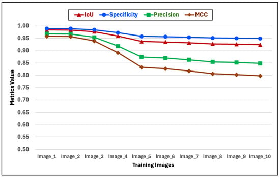
Figure 18. Metrics of the training images with 64-intensity values. The four metrics reported are Interception over Union (IoU), Specificity, Precision, and Matthews Correlation Coefficient (MCC). The calculated metrics are consistent across all images. The resulting metrics lead us to conclude that the encoded images in the training dataset were correctly revealed.

The good results obtained in translating the training images are evident in Figure 19 and Figure 20. Both figures provide the generated images and the metrics Interception over Union, Specificity, Precision and Matthews Correlation Coefficient for the datasets with intensity values of 16, 32, 64, and 256. The average values of the image metrics are high and are shown in the last row of the figures.

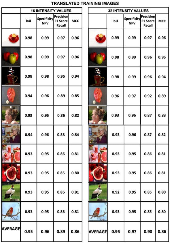
Figure 19. Set of 10 training images translated from the 16- and 32-intensity value datasets and their metrics derived from binary analysis of the images. The metrics for each translated image are shown. These metrics are Intersection over Union (IoU), Specificity, Precision and MCC. The average values of the image metrics are high and are shown in the last row of the figure.

It is interesting to note that, for the training datasets, the sharpness of the translated images is independent of the number of intensity values in the dataset. That is, all training images exhibit a similar degree of sharpness, regardless of the number of intensity values in the dataset. The metrics scores are consistent with this observation.

In Figure 21, we plot the average values of the Specificity, IoU, Precision and MCC metrics for the set of 10 training images. The figure shows that for datsets of 16-, 32-, 64-, and 256-intensity values the metrics take constant values. Except for a slight change in the dataset of 256-intensity values, the metrics remain constant. The consequence of this is that for training images, it is possible to vary the intensity values of the encoded images, and the revealed images will not experience improvement or deterioration as a result. Behind this statement is the fact that the selection of the best model for each dataset was made by choosing the one that showed the best performance in image translation during training. This means that the number of iterations for each dataset was different and that the models were able to perform the number of iterations required to achieve the same level of quality. However, as we will see in the next subsection, this behavior is different for the test datasets.

Figure 20. A set of 10 training images translated from the 64- and 256-intensity datasets showing the metrics derived from the binary analysis of the images. The metrics for each translated image are Intersection over Union (IoU), Specificity, Precision and MCC. The average values of the image metrics are high and are shown in the last row of the figure.

Figure 21. Average values of the metrics derived from a binary analysis for a set of 10 translated training images. The average values for the Specificity, IoU, Precision, and MCC metrics are high for the translated training images and remain constant regardless of the number of intensity values in the dataset. From these experiments, it follows that the sharpness of the translated image does not depend on the intensity values of the dataset. Experiments with test datasets behave differently with respect to the number of intensity values.

Evaluation of translated test images. The metrics applied to evaluate the test images are also Intersection over Union, Specificity, Precision and Mattews Correlation Coefficient. Figure 22 shows the scores for these metrics for the 16- and 32-intensity datasets. Figure 23, on the other hand, shows the same scores for the 64- and 256-intensity datasets. The sharpness of the image varies considerably with the number of intensity values and becomes blurred as the intensity value increases. For the 16-intensity test dataset, the average values of specificity and IoU are 0.95 and 0.93, respectively, while the average values of Precision and MCC are 0.86 and 0.82, respectively. The quality of the translated images for this test dataset is good according to the metrics scores. A similar thing can be said for the specificity and IoU metrics for the 32-intensity test dataset, while Precision and MCC have average values of 0.82 and 0.76, respectively, which is reflected in the fact that these images are less sharp than the 16-intensity dataset.

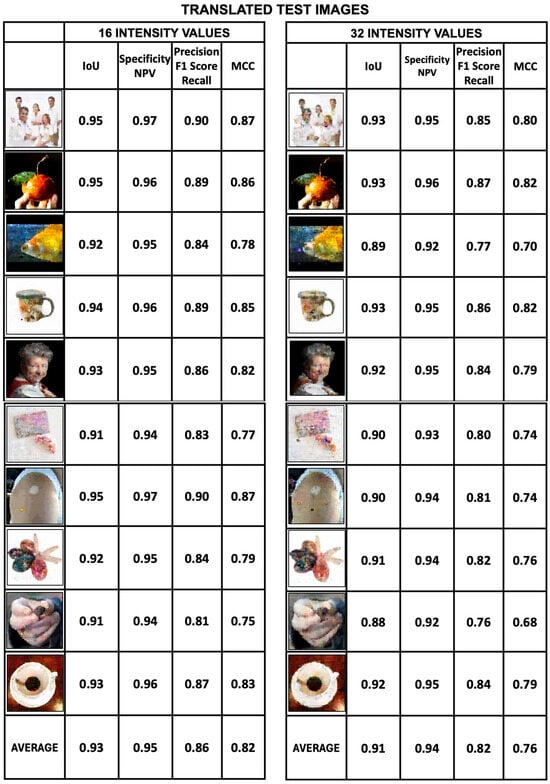
Figure 22. Metrics of a set of 10 test images translated from the 16- and 32-intensity value datasets. The values obtained from the calculated metrics are Intersection over Union, Specificity, Precision and MCC. The images that obtained the highest metric scores are the test datasets with 16-intensity values, and the translated images from this dataset are the ones that show the greatest sharpness. Test image metrics from the 32-intensity dataset indicate that the image quality is lower.

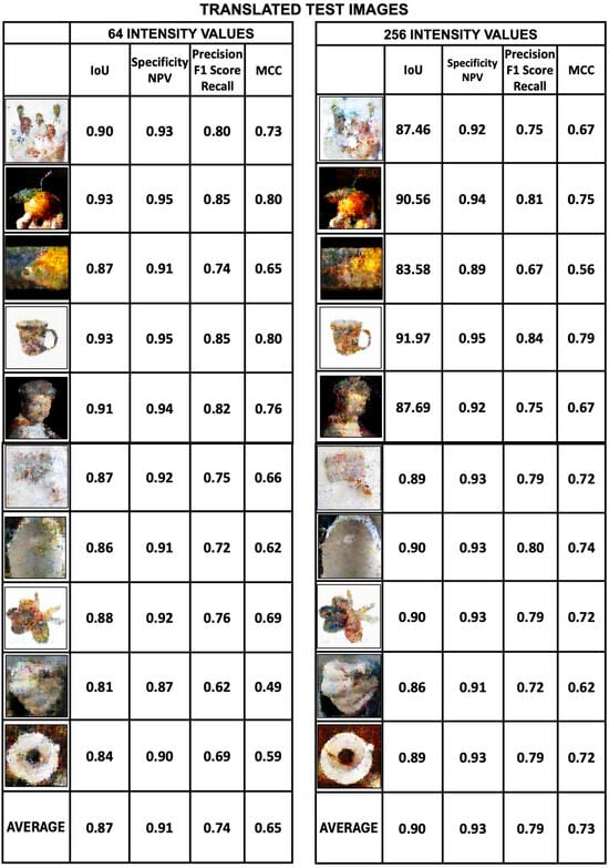
Figure 23. Metrics of a set of 10 test images translated from the 64- and 256-intensity value datasets. For each image the followind metrics are shown: Intersection over Union, Specificity, Precision, and MCC metrics. The images with the lowest metrics are those from the test dataset of 256-intensity values. The sharpness of the image decreases as the number of intensity values increases.

In Figure 24 we plot the average values of the metrics obtained for a set of 10 translated test images. The figure clearly shows the effect of varying the number of intensity values on the test image metrics. Specificity, IoU, Precision, and MCC metrics show the same behavior in all test datasets. The metrics improve as the intensity values of the datasets decrease. Unlike training images, which are not affected by the number of intensity values (Figure 21), the test images are very sensitive to the number of intensity values.

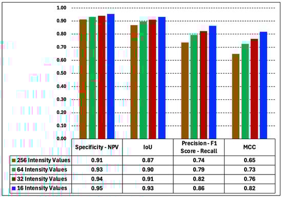
Figure 24. Average values of the metrics derived from a binary analysis for a set of 10 translated test images. Specificity, IoU, Precision, and MCC metrics increase as the number of intensity values decreases for all test datasets. The 16-intensity values dataset has the highest image sharpness, which is consistent with its metric scores.

The cause of this effect in the test datasets is multifactorial. The main cause could be related to image processing in cGANs using a U-Net, which performs an upsampling and downsampling process. In this case, images with lower intensity values can be increased (from 16 to 256 values, for example) and generate a higher-quality image. Figure 25 illustrates the workflow of the datasets and their subsequent integration into the GAN framework. The generator model, which is implemented using a U-Net architecture, is particularly highlighted as the core component responsible for image reconstruction and enhancement. The green box in the figure shows five test datasets with 8, 7, 6, 5, and 4 bits, corresponding to radiometric resolutions of 256, 128, 64, 32, and 16. All test datasets have the same spatial resolution of [256, 256]. The red box shows the U-Net architecture used by the generator model. The upsampling and downsampling process performed by the U-Net is illustrated by the encoder and decoder. As explained in the figure caption, in the cascade decoder stages, the image is progressively reconstructed, achieving higher spatial resolution. At the same time, through the skip connections with the encoder, the radiometric resolution is also enhanced. As a result, test images with lower intensity levels may improve sharpness more than images with higher intensity levels.

Evaluation of the reverse experiment. Double translation. The encoded images generated in the reverse experiment are not suitable for evaluation with the metrics we are using. However, we found a way to recover the unencoded images by double translation. Using the encoded image generated by the reverse experiment as the input image of the normal process, a second translation was performed using the model generated by the training dataset of 16-intensity values (Section 3.1). With the second translation of the encoded image generated by the reverse experiment, it was possible to recover the original image. The images obtained from the second translation can be evaluated using the metrics that we are applying here. Evaluation is performed on the training and test images. Figure 26 shows the results of the application of the metrics to the training images obtained by double translation. The coded images generated in the reverse experiment were revealed using the model generated in the normal procedure that allows the coded images to be translated. Figure 26 shows the metrics Intersection over Union, Specificity, Precision and Mattews Correlation Coefficient. The average values for the Specificity, IoU, Precision, and MCC metrics are 0.95, 0.93, 0.85, and 0.80, respectively. These scores are high and comparable with those of the training images obtained in the normal process (Figure 19 and Figure 20).

Figure 25. The test experiment is illustrated using five image datasets. The main variation among these datasets was the number of available intensity levels. As shown in the green box of the figure, dataset (a) has full radiometric resolution with 256 possible values; in (b), the radiometric resolution was limited to 128-intensity levels; in (c), to 64 levels; in (d), to 32 levels; and in (e), only 16-intensity levels were available. Each dataset could be selected as input to the GAN. In the generator module, a U-Net architecture was employed, as illustrated in the red box of the figure. In the cascade decoder stages, the image is progressively reconstructed, achieving higher spatial resolution. At the same time, through the skip connections with the encoder, the radiometric resolution is also enhanced. This is particularly relevant because, even when input images have low radiometric resolution (e.g., 4 or 5 bits), the model is able to improve the results obtained with full radiometric resolution images.

Figure 26. Reverse experiment. Metrics for the double-translated training images. The average values for the specificity, IoU, precision, and MCC metrics are 0.95, 0.93, 0.85, and 0.80, respectively. These scores are high and comparable with those obtained by the training images in the normal process (Figure 19 and Figure 20) despite having double translation.

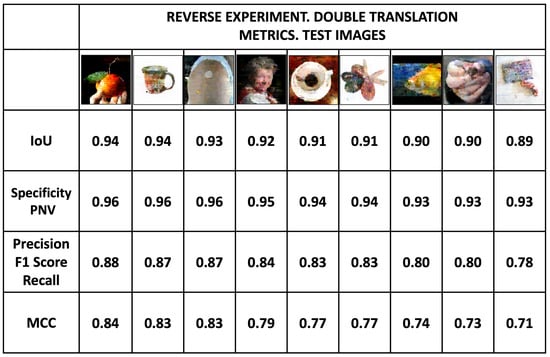
Figure 27 shows images of the test dataset obtained by double translation, and the metrics of Intersection over Union, Specificity, Precision and MCC. Despite the double translation process, the images show a similar quality to the test images with 16-intensity values obtained in the normal process (Figure 22 and Figure 23). The average values of Specificity, IoU, Precision, and MCC metrics are 0.94, 0.92, 0.83, and 0.78, respectively.

Figure 27. Reverse experiment. Metrics of the test dataset images obtained by double translation. Despite the double translation, the metric scores are comparable with those of the test dataset images generated in the normal process. (Figure 22 and Figure 23), despite having double translation.

Analysis of the Complexity of the Method. When scaling the spatial resolution dimensions, the computational cost per iteration increases in a quadratic order. If we increase the resolution from 256 × 256 to 512 × 512, the time and CPU increase four times. The Complexity Analysis can be estimated for cGAN training as follows:

$$C_{train}=O(N_{img}\times E\times n^2\times k^2\times L),$$

(9)

where:

$C_{train}$: Computational Complexity for cGAN training;

$N_{img}$: Number of images in the dataset (1505);

E: Number of Epochs (200);

$n^2$: Pixel number (65,536);

$k^2$: Kernel size (3);

L: Number of U-Net blocks (≈8–10 in Pix2Pix).

This gives a practical complexity of the order of $O({10}^8$–${10}^9)$ operations per Epoch.

Limitations and Potential Applications. Among the limitations, the scalability on higher-resolution images is paramount. The spatial resolution of our images is 256 × 256 pixels, so thinking of images with a resolution of 512 × 512 quadruples the number of operations. If we consider scalability in higher resolution images (e.g., 4K), the increase in the number of operations would be more than 250 times, which can be considered computationally prohibitive. In this scenario, the use of optimizers, such as multi-scale training, patch-based learning, or gradient checkpointing, should be considered to help us work with higher-resolution images.

5. Conclusions

In this work, we have addressed an original problem consisting of revealing images encoded by dynamic S-boxes based on a cryptographically secure pseudo-random number generator. Our results demonstrate that the Pix2Pix cGAN has the ability not only to reveal encoded images but also to emulate the encoding of a real image. The results of experiments in which intensity levels varied between 256, 64, 32, and 16 show that the quality of the revealed test images improves as intensity levels decrease, while the training images do not show a significant change with varying intensity levels. In addition, a reverse experiment was performed in which the input and output images were inverted to generate an encoded image from a real image. The results of this experiment indicate that the cGAN successfully learned to emulate real image encoding according to the S-box technique described in Section 2, a result that was confirmed by performing a second translation of the encoded image that was generated and that allowed the original real image to be recovered. Regarding image quality assessment, the generated images were evaluated using a binary analysis of the images and metrics derived from the confusion matrix. It was found that in the binary analysis technique used, the number of false negatives is equal to the number of false positives, an identity that does not have major implications in images, unlike in biomedical cases, where it does make a big difference. Finaly, the results were evaluated based on four independent metrics: Accuracy, Specificity, MCC, and IoU. The metric results are consistent with each other and show that the quality of the translated training images has virtually identical metric scores, regardless of the intensity levels. Although our manuscript focused on the goal of developing a functional scheme that allows revealing encoded images (digital signals), some potential applications can be visualized, for example, image restoration, and compression, visual encryption and digital security.

References

- Isola, P.; Zhu, J.; Zhou, T.; Efros, A. Image-to-Image Translation with Conditional Adversarial Networks. In Proceedings of the 2017 IEEE Conference on Computer Vision and Pattern Recognition (CVPR), Honolulu, HI, USA, 21–26 July 2017. [Google Scholar]
- Goodfellow, I.; Pouget-Abadie, J.; Mirza, M.; Xu, B.; Warde-Farley, D.; Ozair, S.; Courville, A.; Bingo, Y. Generative Adversarial Nets. In Proceedings of the 28th International Conference on Neural Information Processing Systems, NIPS’14, Montreal, ON, Canada, 8–13 December 2014. [Google Scholar]
- Ding, S.; Wallin, A. Towards recovery of conditional vectors from conditional generative adversarial networks. Pattern Recognit. Lett. 2019, 122, 66–72. [Google Scholar] [CrossRef]
- Choubey, A.; Gajbhiy, S.; Tiwari, R. A Survey Paper on Text Visualization Using Generative Adversarial Network; Book Series Cognitive Science and Technology; Springer: Berlin/Heidelberg, Germany, 2025; Part F 228; pp. 129–140. [Google Scholar] [CrossRef]
- Kasi, G.; Abirami, S.; Lkshmi, R. A Deep Learning Based Cross Model Text to Image Generation using DC-GAN. In Proceedings of the 12th IEEE International Conference on Advanced Computing, ICoAC, Chenai, India, 17–19 August 2023. [Google Scholar]
- Murali, S.; Rajati, M.; Suryadevara, S. Image generation and style transfer using conditional generative adversarial networks. In Proceedings of the 18th IEEE International Conference on Machine Learning and Applications, ICMLA 2019, Boca Raton, FL, USA, 16–19 December 2019. [Google Scholar]
- Al-Adwan, A. Evaluating the Effectiveness of Brain Tumor Image Generation using Generative Adversarial Network with Adam Optimizer. Int. J. Adv. Comput. Sci. Appl. 2024, 15, 512–521. [Google Scholar] [CrossRef]
- Bisht, M.; Gupta, R. Conditional Generative Adversarial Network for Devanagari Handwritten Character Generation. In Proceedings of the 7th International Conference on Signal Processing and Communication, ICSC 2021, Noida, India, 25–27 November 2021. [Google Scholar]
- Balaji, P.; Salian, N.; Nikhil, B.; Narsipura, O. Super-Resolution of Level-17 Images Using Generative Adversarial Networks; Book Series Lecture Notes on Data Engineering and Communications Technologies; Springer: Singapore, 2020; Volume 61, pp. 379–392. [Google Scholar] [CrossRef]
- Chen, J.; Zhang, Y.; Hu, X.; Chen, C. Cascading residual–residual attention generative adversarial network for image super resolution. Soft Comput. 2021, 25, 9651–9662. [Google Scholar] [CrossRef]
- Min-ha-zul, A.; Yousuf, M. StegoPix2Pix: Image Steganography Method via Pix2Pix Networks. In Proceedings of the Fourth International Conference on Trends in Computational and Cognitive Engineering, Tangail, Bangladesh, 18–19 December 2022; Lecture Notes in Networks and Systems. Springer: Singapore, 2023; Volume 618. [Google Scholar] [CrossRef]
- Bonilla-Marín, M.; Tuxpan, J.; Campos-Cantón, E. Alternative method to reveal encoded images via Gaussian distribution functions. Integration 2024, 96, 102166. [Google Scholar] [CrossRef]
- Bonilla-Marín, M.; Tuxpan, J.; Campos-Cantón, E. Visualization of Encoded RGB Images Using Gaussian Distribution Functions. Control and Dynamic Systems Departament, IPICYT, San Luis Potosí, S.L.P., Mexico. 2025; Manuscript to be submitted. [Google Scholar]
- Cassal-Quiroga, B.B.; Campos-Cantón, E. Generation of Dynamical S-Boxes for Block Ciphers via Extended Logistic Map. Math. Probl. Eng. 2020, 2020, 2702653. [Google Scholar] [CrossRef]
- García-Martínez, M.; Campos-Cantón, E. Pseudo-random bit generator based on lag time series. Int. J. Mod. Phys. C 2014, 25, 1350105. [Google Scholar] [CrossRef]
- Russakovsky, O. ImageNet Large Scale Visual Recognition Challenge. Int. J. Comput. Vis. 2015, 115, 211–252. [Google Scholar] [CrossRef]
- Brownlee, J. Generative Adversarial Networks with Python. (e-Book), v1.81. Available online: https://machinelearningmastery.com/generative_adversarial_networks/ (accessed on 18 November 2025).
- Borji, A. Pros and cons of GAN evaluation measures. Comput. Vis. Image Underst. 2019, 179, 41–55. [Google Scholar] [CrossRef]
Disclaimer/Publisher’s Note: The statements, opinions and data contained in all publications are solely those of the individual author(s) and contributor(s) and not of MDPI and/or the editor(s). MDPI and/or the editor(s) disclaim responsibility for any injury to people or property resulting from any ideas, methods, instructions or products referred to in the content. |
© 2025 by the authors. Licensee MDPI, Basel, Switzerland. This article is an open access article distributed under the terms and conditions of the Creative Commons Attribution (CC BY) license (https://creativecommons.org/licenses/by/4.0/).