Abstract
Image distillation is becoming a hot area of machine learning (ML) research because it minimizes the computer resources used for training of convolutional neural networks (CNNs). In this paper, we propose a novel method for image distillation that learns the gradient of the loss function after training a CNN with the original training image. It then modifies the images using the learned gradient and applies K-means clustering to split the modified images into clusters, in a class-wise fashion, and select their centroids as distilled images. We evaluated the capabilities of our method on MNIST, Fashion-MNIST, CIFAR-10, and the Oral Cancer Image Database (OCID) using three CNN models (Baseline, ResNet, and LeNet). The results show that when training the classifiers (CNN) with distilled images, we obtained accuracies of 99.93% for MNIST, 99.46% for Fashion-MNIST, 99.05% for CIFAR-10, and 91.8% for OCID, which are comparable with the results after training with the entire training set. Comparison of our distillation method with existing contemporary methods such as KIP and RTP showed the supremacy of the former even if trained with fewer epochs. A bottleneck of our method is that it works with gradient-based optimizers.
MSC:
62D99; 62H30; 62H35; 68T10
1. Introduction
Deep learning models have achieved remarkable success across various computer vision tasks. However, this success often comes at the cost of requiring large, diverse training datasets, which pose practical challenges, especially in scenarios where computational resources are limited or data storage and processing time are constrained. As deep learning continues to expand to mobile, embedded, and edge computing environments, there is an increasing demand for lightweight training solutions that will preserve the features of the original training set while reducing data size and computer resources.
Dataset distillation is a promising approach to address this challenge. Instead of using the full dataset, distillation methods aim to extract a small yet informative subset of samples that can be used to train models effectively [1,2]. Recent works have explored methods such as gradient matching [3], kernel-based optimization [4], and distribution-aware distillation [5]. Instead of directly distilling the entire original datasets into synthetic images, paper [6] learns a generative model to capture the dataset properties. The generative model, once trained, can produce synthetic images. The study in [7] proposes assigning importance weights to different network parameters during distillation to better preserve crucial information. It matches gradients or parameters between real and synthetic data, but in a way that adapts per-parameter importance. Although these methods show promising results, many of them require a large number of training epochs, numbering in the thousands [8], or complex optimization steps to achieve high accuracy.
Two distillation methods that do not require training iterations are presented in [9,10]. In [9] the authors proposed a technique for distilling time-series data based on a modified form of the principal component analysis (PCA) method [11]. The study in [10] proposed an image distillation method that integrates the Discrete Wavelet Transform (DWT) [12], Modified PCA (M-PCA) [9], and a Sparse Representation Wavelet-based Classification (SRWC) [13]. The last approach was experimentally evaluated on three datasets: digit MNIST [14], Extended YaleB, which contains faces [15], and the ISIC 2020 skin lesion image database [16].
The centroid of a set of images is a concept with the potential to be a part of a distillation procedure because it groups data. One of the most used methods for clustering is K-means, which employs measures of similarity [17]. Further, the K-Spectral Centroid is applied in [18] to determine patterns in time series.
The benefits one may obtain from using distilled images can be summarized as follows: reduced computational cost through training with a small distilled set that carries the training abilities of the entire set and improved learning efficiency through better generalization.
In the present paper, we propose an effective dataset distillation method that combines gradient-based images modification, K-means clustering, and the use of the cluster centroids as distilled images. Figure 1 below is the pictorial description of our method, which distills a set of images that effectively represent the full dataset, enabling model training with fewer images while preserving accuracy.
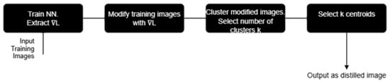
Figure 1.
A flow chart describing the new distillation method. denotes the gradient of the loss function; the clustering is class-wise.
Our method is evaluated on MNIST [14], Fashion-MNIST [19], CIFAR-10 [20], and OCID [21] using three CNN models: Baseline [22], ResNet [23], and LeNet [14]. The experimental results show that our method distills images, which: steady increase classification accuracy when the distillation training epochs increase (Table 1 and Table 2); achieve accuracy comparable to the accuracy obtained when training with the entire original training set (Table 3); and converges faster than contemporary methods like KIP [4] and RTP [24] (Table 4). Notably, the new method achieved 99.20%, significantly outperforming the competitors on CIFAR-10 image databases.
The key contribution of our paper is the development of a novel distillation method, which first trains a CNN with the original training images and uses the norm of the gradient of the loss function, at the last training epoch, to modify the training images. Then the K-means method clusters the modified images and selects the centroid of each cluster as a distilled image. Note that the image modification and clustering methods work consecutively and the user selects the number of clusters.
The major advantage that comes from this contribution is the significant reduction in computational cost, as it greatly decreases the number of training images needed. For example, as shown in Table 3, training the Baseline CNN with 100 images distilled from MNIST provided an accuracy of 97.51%, while training with 60,000 original training images showed 99.36%. In both experiments 200 epochs were used.
In addition, this paper is organized as follows. Section 2 analyzes contemporary methods from the field of image distillation; Section 3 in its first part develops the new method for image modification with the help of the gradient of the loss function of a CNN; Section 3.2 develops the step-by-step algorithm, while Section 3.3 introduces the basics of the K-means method to cluster and modify images; Section 4 sets up the experiments; Section 5 describes their results; and the paper ends with Section 6 and Section 7, which analyze the advantages and bottlenecks as well as formulate the future work.
2. Contemporary Methods in the Field
Although many methods for dataset distillation have been proposed, most of them have clear drawbacks that limit their practical use. One of the main approaches for data distillation is gradient matching, proposed by Zhao et al. [3]. Instead of selecting real data points, this method produces synthetic examples whose gradients of the loss function closely match those obtained when training on the full dataset. In practice, synthetic samples are optimized so that their gradients align with the optimization direction of the original training dataset. The authors showed that even ten synthetically created images per class can rival models trained on full training datasets.
Another distillation method is grounded in kernel-based condensation, and particularly on the Kernel Inducing Point (KIP) method presented by Nguyen et al. [4]. KIP utilizes kernel ridge regression to find an optimal subset of training images, which can act as a proxy for the whole dataset. The method is attractive for federated or privacy-sensitive tasks, although often it requires thousands of training epochs.
In another approach, differential privacy has been combined with distillation. DP-KIP was suggested by Vinaroz and Park [8], which incorporates formal privacy assurance to make KIP capable of protecting sensitive information during condensation. Although suitable for privacy-sensitive tasks, DP-KIP is computationally expensive. Gradient matching [3], for example, showed that synthetic images could replace large datasets, but it requires heavy optimization and long training times, which make the method less efficient. Kernel-based approaches such as KIP and its privacy-preserving version DP-KIP have also reported high results, but they are computationally expensive and often need thousands of epochs to converge. Other techniques used wavelet transforms, PCA, and sparse representation to reduce training dataset size but add complexity and do not always balance accuracy with efficiency [13].
These limitations highlight the need for better classifier generalizing and balancing distillation. A survey on a number of contemporary methods for image distillation is presented in [24].
Our method addresses these issues of high computational cost, prolonged training time, and limited adaptability in existing dataset distillation approaches by using gradient-based image modification, after training an NN with the original samples. Next, the K-means method clusters the modified images and selects the clusters’ centroids as distilled images. Training with distilled images avoids costly model optimization with the original images and still achieves accuracy close to that of the full datasets. Because the training with distilled images requires fewer resources, the classification process converges faster and maintains strong performance. Thus, our method provides more balanced and scalable alternative to existing approaches.
3. The New Method for Image Distillation
In this section, we will detail the new method for distillation, which comprises two steps: first is the modification of the training images using the gradient of the loss function of a neural network (NN), and then K-means clusters the modified images and selects the clusters’ centroids as distilled images, as shown in Figure 1.
3.1. Image Modification with the Gradient of the Loss Function
As mentioned above, the new method first modifies the image using the gradient of the loss function (see Figure 1). To do so a CNN with a gradient-based learning method is trained for a number of epochs on the full training set. After the training is completed, the method collects the last gradient value of the loss function (Equation (1)). These gradients highlight the discriminative features of each image that are most relevant for classification.
In the standard gradient descent method, the model weights are updated iteratively as follows:
where
- : The weight between neuron i and neuron j at iteration t (epochs);
- : The learning rate, which controls the step size of the update;
- : The gradient of the loss function L with respect to the weight . Here, is the output predicted by the CNN for input i; is the ground truth (target) output for input i.
At the end of the CNN training process, our method takes the norm of the gradient of the loss function in Equation (1) and applies it to modify the training images in a pixel-wise fashion. For a pixel at position in the k-th image, the new pixel value is calculated as follows:
where
- : Pixel value at position in the u-th image, where i = 1, …, M and j = 1, …, N, where M and N are the sizes of the current image, while u = 1, …, p counts the images in the training set;
- The rest of the terms remain the same as in Equation (1).
Applying Equation (2) to the p training images allows the method to modify them. Two examples of modified images after 200 and 600 epochs are shown in Figure 2.
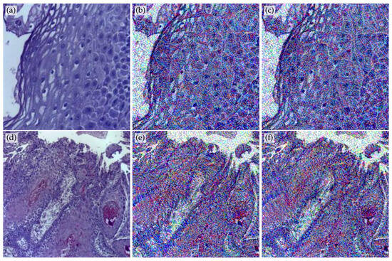
Figure 2.
(a) Original non-cancer image from the OCID image database [21]; (b) its modified version after 200 training epochs with the original training images; (c) modified version after 600 training epochs; and (d–f) cancer OCID original image, named OSCC, and its modified version after 200 and 600 epochs.
3.2. Step-by-Step Outline of the Proposed Method
A clear step-by-step description of the proposed image distillation process is provided below to improve clarity regarding how the loss function gradient is calculated and applied and which parameters remain constant during modification.
- A convolutional neural network (CNN) is first trained on the original dataset for a fixed number of epochs using a gradient-based optimizer (e.g., Adam).
- After training, the norm of the loss function gradient is computed, using Equation (1), for each training image.
- Each training image is then modified with the help of Equation (2), where is the learning rate.
- The learning rate, network architecture, and optimizer parameters remain constant throughout the modification process to maintain consistency.
- The modified images , are grouped class-wise, and the K-means clustering algorithm is applied to every class to select the cluster centroids as the final distilled images.
The clustering approach was validated on the OCID training set, from which 10 representative normal and 10 cancer images were distilled from the 4946 training samples. Figure 3 shows one example each of a distilled normal and a distilled cancer image.
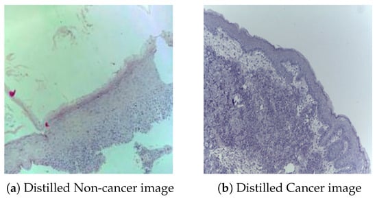
Figure 3.
Shown are 2 out of the 20 distilled images from the entire set of 4946 original training images. The size of the original and the distilled images is 224 × 224 pixels.
3.3. K-Means Clustering for Distillation
A way to make datasets smaller is by picking real samples that may represent the whole data. K-means is often used for this task because it groups data by implementing a measure of similarity and uses centroids as summaries. Coates and Ng [17] showed that the above-mentioned approach helps with feature learning, while Zheng [25] applied K-means for adaptive image segmentation to improve the accuracy of region detection in complex images. However, clustering alone can miss some important details, so it works better when combined with image modification.
Once the training images in all classes are modified, our approach applies the K-means method to cluster the images modified by Equation (2) in a class-wise fashion. The basics of the class clustering are given below.
Assume a set of observations where and are images of the same size. K-means clustering aims to partition the n observations into sets so as to minimize the total variance within the cluster, that is, the sum of squared Euclidean distances between each data point (images in our case) and the centroid of its assigned cluster. Formally, the objective is to find
where is the mean of the i-th cluster (also called centroid) of points (images) in ; i.e.,
is the size of the cluster and denotes the norm, while is the j-th image in the i-th cluster. Equation (3) is equivalent to minimizing the pairwise squared deviations of points (images) in the same cluster [26,27].
The clusters’ centroids selected from each class are the distilled images from this class. The distillations from all classes are used to train CNN classifiers such as Baseline, ResNet, and LeNet. The distilled sets from all classes represent a smaller yet diverse dataset made of only the most representative images, which reduces training time while keeping model accuracy high, as seen in Table 1, Table 2 and Table 3 and Table 5.
4. Experimental Setup
In this section, we explain how we validated the advantages of our new image distillation method using different datasets, models, and settings.
4.1. Datasets
For the purpose of validation, we used four popular public image datasets:
- MNIST [14]: Handwritten digits from 0 to 9, grayscale, 28 × 28 pixels, 60,000 training and 10,000 test images.
- Fashion-MNIST [19]: Grayscale images of clothing items such as shirts, shoes, and bags. Same size and structure as MNIST.
- CIFAR-10 [20]: Colored 32 × 32 images across 10 classes like airplanes, birds, and cats. Contains 50,000 training and 10,000 test images.
- OCID [21]: Color histopathologic images (which we transformed into a database of image sizes , which can be found at https://www.etamu.edu/projects/augmented-image-repository/?redirect=none, 25 February 2025) of oral tissue with ground truth labels and cancerous-OSCC and non-cancerous classes. The entire set is split to 4946 training, 120 validation, and 126 test images across the two classes.
In this study, we trained three CNNs, Baseline [22], ResNet [23], and LeNet [14], to recognize images and collect the gradient values of the loss function after training with the original images. We distill a number of m images per class in a class-wise fashion. Hence, the label of the distilled images is the same as the label of the class we are distilling from. Our new image distillation method applies for CNNs whose optimizer is the gradient descent method (GDM) [28] or its modifications like stochastic GDM (SGDM), Adam, or modified Adam. After training the corresponding classifier with the entire original training data, we extract the value shown in Equation (4) from Equation (1) and apply it in Equation (2) for image modification.
Note, the method applies the value from Equation (4) to modify the images in the entire training dataset. Further, we employ the K-means method [26] in a class-wise fashion to split every class into k clusters and determine their centroids. Note that the number k is selected by the user.
4.2. Models Evaluated
Convolutional neural networks (CNNs) are widely used in computer vision because they can automatically learn patterns like edges, shapes, and textures from images. They use convolution layers to capture local features, pooling layers to reduce dimensions, and fully connected layers for classification. CNNs are powerful because they need less training samples to capture features compared to traditional models. We validated the new image distillation method using three different CNN architectures:
- Baseline CNN [22]: This is a very small network with about four layers in total: two convolution layers with the ReLU activation function, one max pooling layer, and one dense softmax output layer. The dense output layer usually has around 128–256 neurons, depending on the dataset size. It is lightweight classifier that provides a baseline for comparison.
- ResNet [23]: The version we used has 34 layers, which include many convolution layers grouped into residual blocks, with batch normalization and the ReLU activation function inside each block. The final fully connected layer usually has 1000 neurons (for ImageNet classification), but can be adjusted to match the dataset classes. In total, the network contains over 20 million parameters, making it very expressive and computationally heavy.
- LeNet [14]: This model has seven layers in total. It starts with two convolution layers (with activation functions), each followed by average pooling, then three fully connected layers, and ends with a softmax classifier. The fully connected part includes about 120 neurons in the first layer, 84 neurons in the second layer, and an output layer that usually matches the number of classes (e.g., 10 neurons for digit-MNIST dataset classification). In general, LeNet has around 60,000 parameters.
4.3. Training Setup
We trained the above models implementing the following settings:
- Framework: All models were implemented and trained in Google Colab using TensorFlow/Keras.
- Epochs: Each model was trained for a number of epochs that varied from 200 to 1000, depending on the particular experiment.
- Batch size: This is set to 32 for all experiments.
- Loss function: Categorical cross-entropy was used since all tasks were multiclass classification problems:where N is the number of training samples, C is the number of classes, and is the ground truth label of the input sample with index i. Further, we defineis the predicted probability for the i-th sample to belong to class .
- Optimizer: Adam optimizer with a learning rate of 0.001
All experiments were conducted in Google Colab using TensorFlow/Keras with GPU acceleration. The key parameters (, number of k-means clusters, and distilled images per class) were determined empirically through preliminary validation to achieve a balance between accuracy and computational efficiency.
All CNN models were trained using the Adam optimizer with a fixed learning rate of 0.001 and a batch size of 32. The number of training epochs varied from 200 to 1000 depending on the experiment. No learning rate decay was applied to ensure consistent comparison across models.
For comparison, we measured the classification outcomes with the statistical metrics: accuracy = AC, sensitivity = SE, and specificity = SP, implemented in scikit-learn [29].
where TP = True Positives, TN = True Negatives, FP = False Positives, and FN = False Negatives.
5. Experimental Results
Table 1, Table 2, Table 3, Table 4 and Table 5 summarize the accuracy of the three models for different training epochs and numbers of distilled images per class. One may notice from Table 1 and Table 2 that increasing the number of training epochs, for the purpose of distillation, increases the accuracy of classification. Table 3 compares the classification accuracy after training with 60,000 or 50,000 original training images, depending on the dataset, and 100 distilled images. One can tell that the gap between the classification accuracies if trained with original and distilled images narrowed significantly with the increase in the training epochs for distillation. This underlines the importance of the distilled images for ML methods that require a large number of training epochs.
Further, Table 4 indicates that our method outperformed two contemporary approaches for image distillation. Table 5 extends our analysis to the medical image database OCID, evaluated using three convolutional neural networks (ResNet, Baseline, and LeNet). Two experimental scenarios were implemented: the first employed 20 distilled images (10 per class), while the second used the full dataset containing 2437 normal and 2511 cancerous oral images. For the ResNet model, the entire original OCID dataset achieved accuracies between 91.29% and 91.54% across 200–600 epochs, whereas training with distilled images yielded accuracies ranging from 72.50% to 91.80%. The gradual improvement with increasing the training epochs and the convergence toward full-dataset performance indicate that the distilled subset retains essential distinctive features even for complex medical imagery. Note that the classification after training with 20 distilled images showed a slightly higher accuracy than training with the entire set of 4.948 original training images. These results further confirm that our new method for dataset distillation can substantially reduce computational resources while maintaining high diagnostic accuracy.

Table 1.
Accuracy (in %) of classification of the original test set after training with 100 (10 per class) distilled images and using 200–600 epochs in the far-right columns. The highest result in every row is in bold.
Table 1.
Accuracy (in %) of classification of the original test set after training with 100 (10 per class) distilled images and using 200–600 epochs in the far-right columns. The highest result in every row is in bold.
| Images/Class | Dataset | Models | 200 | 300 | 400 | 500 | 600 |
|---|---|---|---|---|---|---|---|
| 10 | MNIST | Baseline | 97.51 | 98.44 | 98.58 | 99.07 | 99.67 |
| 10 | MNIST | ResNet | 96.60 | 97.31 | 98.22 | 98.41 | 98.49 |
| 10 | MNIST | LeNet | 99.36 | 99.51 | 99.57 | 99.06 | 99.73 |
| 10 | FASHION | Baseline | 96.80 | 97.58 | 98.03 | 98.42 | 99.52 |
| 10 | FASHION | ResNet | 96.73 | 97.71 | 98.13 | 98.45 | 98.75 |
| 10 | FASHION | LeNet | 96.50 | 97.93 | 98.24 | 98.43 | 98.61 |
| 10 | CIFAR-10 | Baseline | 87.91 | 91.85 | 93.66 | 94.73 | 95.62 |
| 10 | CIFAR-10 | ResNet | 91.79 | 93.48 | 94.99 | 96.14 | 96.36 |
| 10 | CIFAR-10 | LeNet | 94.29 | 96.07 | 97.93 | 97.71 | 98.62 |
Table 2.
Accuracy (in %) of classification of the original test set after training with 500 (50 per class) distilled images and using 200–600 epochs in the far-right columns. The highest result in every row is in bold.
Table 2.
Accuracy (in %) of classification of the original test set after training with 500 (50 per class) distilled images and using 200–600 epochs in the far-right columns. The highest result in every row is in bold.
| Images/Class | Dataset | Models | 200 | 300 | 400 | 500 | 600 |
|---|---|---|---|---|---|---|---|
| 50 | MNIST | Baseline | 98.41 | 98.73 | 99.04 | 99.24 | 99.26 |
| 50 | MNIST | ResNet | 98.57 | 99.21 | 99.44 | 99.50 | 99.59 |
| 50 | MNIST | LeNet | 99.55 | 99.70 | 99.81 | 99.84 | 99.87 |
| 50 | FASHION | Baseline | 96.69 | 97.51 | 98.24 | 98.48 | 99.65 |
| 50 | FASHION | ResNet | 96.70 | 97.88 | 98.18 | 98.61 | 98.81 |
| 50 | FASHION | LeNet | 97.50 | 98.43 | 98.79 | 99.02 | 99.21 |
| 50 | CIFAR-10 | Baseline | 84.98 | 88.34 | 91.49 | 92.74 | 94.33 |
| 50 | CIFAR-10 | ResNet | 89.94 | 93.15 | 94.79 | 95.21 | 96.34 |
| 50 | CIFAR-10 | LeNet | 95.63 | 97.59 | 97.93 | 98.46 | 98.56 |
Table 3.
AC (in %) comparison when training the Baseline network with 6000 images per class for MNIST and Fashion and 5000 images per class for Cifar-10, with 10 distilled samples per class for the three of them.
Table 3.
AC (in %) comparison when training the Baseline network with 6000 images per class for MNIST and Fashion and 5000 images per class for Cifar-10, with 10 distilled samples per class for the three of them.
| Images per Class | MNIST/Epoch | CIFAR-10/Epoch | Fashion/Epoch |
|---|---|---|---|
| 6000/5000 | 96.96/10 | 63.64/10 | 88.89/10 |
| 10 | 58.51/10 | 31.70/10 | 53.70/10 |
| 6000/5000 | 98.26/20 | 71.53/20 | 87.57/20 |
| 10 | 73.66/20 | 38.85/20 | 70.55/20 |
| 6000/5000 | 99.36/200 | 93.30/200 | 98.49/200 |
| 10 | 97.51/200 | 87.91/200 | 96.80/200 |
Table 4.
Comparison of classification ACs (in %) after training with images distilled by our method and contemporary competitors. The highest result per row is in bold in the three rightmost columns. We used the notation N1/N2, where N1 denotes AC in % while N2 denotes the number of epochs.
Table 4.
Comparison of classification ACs (in %) after training with images distilled by our method and contemporary competitors. The highest result per row is in bold in the three rightmost columns. We used the notation N1/N2, where N1 denotes AC in % while N2 denotes the number of epochs.
| Images/Class | Dataset | Ours/N2 | KIP-Scatternet/N2 [8] | RTP/N2 [24] |
|---|---|---|---|---|
| 10 | MNIST | 99.86/1000 | 99.0/1000 | 99.3/NA |
| 50 | MNIST | 99.93/1000 | 99.4/2000 | 99.4/NA |
| 10 | FASHION | 99.29/1000 | 89.5/2000 | 90.0/NA |
| 50 | FASHION | 99.46/1000 | 90.6/2000 | 91.2/NA |
| 10 | CIFAR-10 | 99.20/1000 | 66.2/1000 | 71.2/NA |
| 50 | CIFAR-10 | 99.05/1000 | 68.5/1000 | 73.6/NA |
Table 5.
Accuracy, sensitivity, and specificity (in %) of classification of the original testing images after training with the entire dataset and 20 (10 per class) distilled OCID images for different training epochs with ResNet CNN. The highest value in the accuracy columns is in bold.
Table 5.
Accuracy, sensitivity, and specificity (in %) of classification of the original testing images after training with the entire dataset and 20 (10 per class) distilled OCID images for different training epochs with ResNet CNN. The highest value in the accuracy columns is in bold.
| Epochs | Entire Original OCID | Distilled OCID | ||||
|---|---|---|---|---|---|---|
| Accuracy | Sensitivity | Specificity | Accuracy | Sensitivity | Specificity | |
| 200 | 91.40 | 84.21 | 87.10 | 72.50 | 76.84 | 58.06 |
| 300 | 91.52 | 76.68 | 87.09 | 91.58 | 67.37 | 58.06 |
| 400 | 91.29 | 70.52 | 90.32 | 91.80 | 67.37 | 61.29 |
| 500 | 91.45 | 86.32 | 87.10 | 91.76 | 70.53 | 58.06 |
| 600 | 91.54 | 71.58 | 87.10 | 91.65 | 72.63 | 54.84 |
The confusion metrics and ROC for classification of the OCID testing set when ResNet was trained with 20 images for 600 epochs are shown in Figure 4 below.
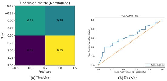
Figure 4.
Performance evaluation of the ResNet model trained on the distilled OCID dataset: (a) normalized confusion matrix and (b) receiver operating characteristic (ROC) curve. The normalized confusion matrix shows high diagonal values (light-green) of 0.52 (true normal predicted as normal) and (yellow) 0.65 (true cancer predicted as cancer) and lower off-diagonal values (dark-green) of 0.48 (normal misclassified as cancer) and 0.35 (purple) (cancer misclassified as normal), indicating accurate class predictions with limited misclassification. The ROC curve was computed using the predicted class probabilities from the test set, and the area under the curve () was obtained via trapezoidal integration of the ROC curve using the roc_curve and auc functions from scikit-learn. This AUC value demonstrates good discriminative ability between normal and cancer images, confirming that the distilled dataset retained meaningful diagnostic features.
6. Discussion
The main contribution of this study is the development of a new method for image distillation. The method works by first training a neural network with a gradient-based optimizer using the original training samples. Then it takes the norm of the gradient of the loss function of the classifier and uses it to modify the training images. In the next stage, the modified images are clustered with the K-means method and the centroids of the clusters are taken as distilled images.
The ResNet model trained on the distilled OCID dataset achieved AUC ≈ 0.81, demonstrating a good discriminative ability between normal and cancer images. Although some misclassification occurred, the model retained strong generalization despite the reduced training data.
The main benefit of this approach is that it saves computing power by substantially cutting down the number of training images used for classification. For example, as shown in the bottom two rows of Table 3, training with only 100 distilled images using 200 epochs provided almost the same accuracies as training with the full 60,000 original images. In the case of MNIST, training with the 100 distilled images gives 1.85% lower accuracy. For Fashion the difference is 1.69%, while for Cifar-10 when trained with 100 distilled images, the classification is 5.39%, but this is offset by the huge difference between the 60,000/50,000 and 100 training images.
Despite its effectiveness, the method has a few limitations. It requires an initial full CNN training to obtain loss gradients, causing a one-time computational overhead. Its performance also depends on stable model convergence; weakly trained networks may yield poor gradient information, which will negatively affect the distillation. Also, the approach applies only to gradient-based optimizers such as SGD or Adam and has been tested mainly on small to medium datasets. Hence, our future work will focus on improving scalability and reducing this initial overhead.
The rationale behind our choice to develop a new gradient-based image modification method is the following. We assume that the value of the gradient of the loss function at the last training epoch will “carry and add” to every training image under modification information from the other training images. Then, we apply the K-means method to every class of modified images and use the centroid of every cluster as a distilled image, to which is assigned the label of the class that the cluster belongs to. Our choice falls on the K-means clustering because the centroid represents all elements in the cluster.
A method that involves the gradient of the loss function is the KIP-Scatternet method [8]. It applies the Kernel Induction Point (KIP) technique, which randomly initializes the support dataset and then iteratively refines it by minimizing the kernel ridge regression [8]. During training, is updated using a gradient-based optimization method until some convergence criterion is satisfied. KIP-Scatternet preserves privacy, whereas our method does not aim to do so during the data modification phase. However, in terms of classification accuracy, our proposed distillation method outperforms KIP-Scatternet when classifying image databases such as MNIST, FASHION, and CIFAR-10 (see Table 4).
Another method we compare with and outperform in accuracy (see Table 4) is the RTP method [24]. It is composed of two main components: the first one formulates the data distillation problem with the help of memory and addressing matrices, and the second one employs empirical aspects of the back-propagation through time framework, which improves classification accuracy and outperforms single-step gradient matching methods.
7. Conclusions
The experimental results presented in this paper show that our image distillation method is effective, even when training with a small number of images per class. As shown in Table 1 and Table 2, our method achieved high accuracy when training the classifiers on the three datasets, MNIST, Fashion-MNIST, and CIFAR-10, using only 100 or 500 distilled images. For example, the rightmost column of Table 1 presents results when the classifiers were trained on 100 distilled images for 600 epochs. The Baseline model achieved 99.67% on MNIST, while LeNet had the highest accuracy of 99.73%. For Fahiom-MNIST, Baseline achieved the highest accuracy with 99.52%, while LeNet attained 98.75%. Also, the latter CNN reached 98.62% on CIFAR-10. We present same experiment in Table 2 but using 50 distilled images per class for training, and the accuracies obtained clearly show that increasing the number of training distilled images does not always increase classification accuracy. In addition, one may observe from Table 1, Table 2 and Table 3 that increasing the number of training epochs for image distillation and classification significantly improves the classification accuracy. Moreover, increasing epochs allowed the accuracy of models trained on distilled images to approach that of models trained on the full dataset, while using about 600 times fewer training images. This fact demonstrates that the proposed new distillation method not only reduces computational cost but also maintains robust classification performance.
Table 3 highlights how well our distilled datasets train models if compared to the models trained on the full dataset. Even though models trained on the full MNIST, CIFAR-10, and Fashion-MNIST sets are trained on many more images, our distilled sets still achieved comparable accuracy when trained for longer. For instance, training with 100 distilled images for 200 epochs using the Baseline CNN gave 97.51% on MNIST and 96.80% on Fashion-MNIST, which are close enough to the full-data performance of 99.36% and 98.49%, respectively. This highlights the strength of our distillation method in reducing training data while maintaining high performance.
We also compared our method with two recent approaches: KIP-Scatternet [8] and RTP [24], see Table 4. Our method outperformed both while requiring fewer epochs for training and distillation, For example, on CIFAR-10 using 50 distilled images per class for training, our method reached 99.05%, compared to 68.5% for KIP-Scatternet [8] and 73.6% for RTP [24]. The same holds for MNIST with 99.93% and Fashion with 99.46% when trained with 50 distilled images per class. In particular, “A Comprehensive Survey on Dataset Distillation (RTP)” [24] did not report the number of training epochs they trained with, making it difficult to fully compare the efficiency of their method with ours. In contrast, we clearly report both accuracy and epochs, showing that our method reaches peak performance with fewer training steps. As shown in Table 5, the proposed method achieved high classification accuracy across all datasets while using fewer images.
Training ResNet on the entire original training OCID dataset required approximately 3 h and 21 min, whereas training on the distilled dataset for the same 600 epochs and same CNN with the same parameters, was completed in 1 h and 3 min, which demonstrates a substantial reduction in computational time.
Table 5 shows that the models trained on the distilled oral cancer image dataset (OCID) perform very close to, and in some cases better than, the images trained on the entire OCID dataset. For instance, the ResNet model achieved accuracies between 91.29% and 91.54% on the full dataset, while training on distilled images produced accuracies ranging from 72.50% to 91.80%. Note that the latter accuracy, which was obtained when trained with 20 distilled images, is slightly higher than the accuracies obtained when training with the 4,948 original images. These findings demonstrate that the distilled subsets retain essential image features useful for accurate classification, even in challenging medical imaging tasks. Overall, the results confirm that our distillation approach significantly reduces data and computational resources while maintaining strong generalization and diagnostic performance across diverse datasets.
The findings of Figure 4 indicate that the proposed distillation approach can effectively preserve classification performance, as evidenced by the ResNet model’s AUC = 0.81 on the OCID dataset; the model demonstrated good discriminative ability, confirming that essential diagnostic features were successfully retained after data reduction.
A constraint of our distillation method is that it applies to networks whose optimizers are gradient-based. Note that we used medium-sized image datasets, MNIST, Fashion-MNIST, and CIFAR-10, to validate our approach. In future work, we plan to test our method on datasets with a large number of classes, such as CIFAR-100, and also on smaller datasets like Binary MNIST and Fashion Binary to explore its performance at both ends of the data spectrum.
A path to improve our method could be the replacement of the K-means with the K-Spectral Centroid method [18]. Also, convergence and computational cost under varying k-values will be examined in our future studies. Finally, we are interested in applying our distillation approach to more medical image datasets in the future. This would help to evaluate how well the method works in real-world applications such as disease diagnosis, where data can be limited and imbalanced.
Author Contributions
Conceptualization, N.M.S.; methodology, N.M.S.; software N.N.E.; validation N.N.E.; formal analysis, N.M.S. and N.N.E.; investigation, N.M.S. and N.N.E.; writing the original draft, N.N.E.; writing—review and editing, N.M.S. and N.N.E.; visualization, N.N.E.; supervision, N.M.S. All authors have read and agreed to the published version of the manuscript.
Funding
This research received no external funding.
Data Availability Statement
The original data presented in the study are openly available in: Fashion MNIST-GitHub GitHub https://github.com/zalandoresearch/fashion-mnist; Digit-MNIST https://github.com/cvdfoundation/mnist; CIFAR-10 https://www.cs.toronto.edu/~kriz/cifar.html; and HistopathologicOral Cancer Image Database (OCID) https://www.kaggle.com/datasets/ashenafifasilkebede/dataset (all accessed on 27 February 2025).
Conflicts of Interest
The authors declare no conflicts of interest.
Abbreviations
The following abbreviations are used in this manuscript:
| ML | Machine Learning |
| OCID | Oral Cancer Image Database |
| CNN | Convolutional Neural Network |
| KIPs | Kernel Inducing Points |
| AC | Accuracy |
| SE | Sensitivity |
| SP | Specificity |
References
- Nguyen, T.; Tran, T. Dataset distillation with informative samples for efficient deep learning. Adv. Neural Inf. Process. Syst. (NeurIPS) 2020, 33, 1–13. [Google Scholar]
- Yu, R.; Liu, S.; Wang, X. Dataset distillation: A comprehensive review. IEEE Trans. PAMI 2024, 46, 150–170. [Google Scholar] [CrossRef] [PubMed]
- Zhao, B.; Mopuri, K.R.; Bilen, H. Dataset condensation with gradient matching. In Proceedings of the International Conference on Learning Representations (ICLR), Online, 3–7 May 2021; pp. 1–15. [Google Scholar]
- Nguyen, T.; Chen, Z.; Lee, J. Dataset meta-learning from kernel ridge-regression. In Proceedings of the International Conference on Learning Representations (ICLR), Online, 3–7 May 2021; Available online: https://openreview.net/pdf?id=l-PrrQrK0QR (accessed on 25 February 2025).
- Zheng, Z.; Su, X.; Wu, C.; Jia, X. Distribution-aware dataset distillation for efficient image restoration (TripleD). arXiv 2025, arXiv:2504.14826. [Google Scholar]
- Wang, K.; Gu, J.; Zhang, H.; Zhou, D.; Zhu, Z.; Jiang, W.; You, Y. DiM: Distilling Dataset into Generative Model. In Lecture Notes in Computer Science, Proceedings of the ECCV Workshops (19), Milan, Italy, 29 September–4 October 2024; Springer: Cham, Switzerland, 2024; Volume 15641, pp. 42–59. [Google Scholar]
- Li, G.; Togo, R.; Ogawa, T.; Haseyama, M. Importance-Aware Adaptive Dataset Distillation (IADD). Neural Netw. 2024, 173, 106236. [Google Scholar] [CrossRef]
- Vinaroz, M.; Park, M. Differentially private kernel inducing points using features from ScatterNets (DP-KIP-ScatterNet) for privacy preserving data distillation. Trans. Mach. Learn. Res. 2024, 1–15. Available online: https://openreview.net/pdf?id=84M8xwNxrc (accessed on 25 February 2025).
- Sirakov, N.M.; Shahnewaz, T.; Nakhmani, A. Training Data Augmentation with Data Distilled by Principal Component Analysis. Electronics 2024, 13, 282. [Google Scholar] [CrossRef]
- Sirakov, N.M.; Ngo, L.H. Automatic Image Distillation with Wavelet Transform and Modified Principal Component Analysis. Electronics 2025, 14, 1357. [Google Scholar] [CrossRef]
- Yang, J.; Zhang, D.; Frangi, A.F.; Yang, J.Y. Two-dimensional PCA: A new approach to appearance-based face representation and recognition. IEEE Trans. PAMI 2004, 26, 131–137. [Google Scholar] [CrossRef] [PubMed]
- Daubechies, I. Ten Lectures on Wavelets; SIAM: Philadelphia, PA, USA, 1992. [Google Scholar]
- Ngo, L.H.; Luong, M.; Sirakov, N.M.; Le-Tien, T.; Guerif, S.; Viennet, E. Sparse representation wavelet based classification. In Proceedings of the 2018 25th IEEE International Conference on Image Processing (ICIP), Athens, Greece, 7–10 October 2018; pp. 2974–2978. Available online: https://www.proceedings.com/content/042/042295webtoc.pdf (accessed on 20 February 2025).
- LeCun, Y.; Bottou, L.; Bengio, Y.; Haffner, P. Gradient-based learning applied to document recognition. Proc. IEEE 1998, 86, 2278–2324. [Google Scholar] [CrossRef]
- Georghiades, A.S.; Belhumeur, P.N.; Kriegman, D.J. From few to many: Illumination cone models for face recognition under variable lighting and pose. IEEE Trans. PANI 2001, 23, 643–660. [Google Scholar] [CrossRef]
- Codella, N.C.; Gutman, D.; Celebi, M.E.; Helba, B.; Marchetti, M.A.; Dusza, S.W.; Kalloo, A.; Liopyris, K.; Mishra, N.; Kittler, H.; et al. Skin Lesion Analysis Toward Melanoma Detection: A Challenge at the International Symposium on Biomedical Imaging (ISBI). ISIC 2020 Challenge Dataset. 2020. Available online: https://www.isic-archive.com (accessed on 20 February 2025).
- Coates, A.; Ng, A.Y. Learning feature representations with k-means. In Neural Networks: Tricks of the Trade; Montavon, G., Orr, G.B., Müller, K.R., Eds.; Springer: Berlin/Heidelberg, Germany, 2012; pp. 561–580. [Google Scholar]
- Liang, Y.; Qiu, H.; Wang, J.; Zhu, Y.; Zhao, K.; Li, Y.; Liu, Z.; Song, J.; Yang, Y.; Kou, Y. Automated identification of ground kinematic patterns based on InSAR time series displacement and K-SC clustering. Eng. Geol. 2025, 357, 108367. [Google Scholar] [CrossRef]
- Xiao, H.; Rasul, K.; Vollgraf, R. Fashion-MNIST: A novel image dataset for benchmarking machine learning algorithms. arXiv 2017, arXiv:1708.07747. [Google Scholar] [CrossRef]
- Krizhevsky, A. Learning Multiple Layers of Features from Tiny Images; Technical Report; University of Toronto: Toronto, ON, Canada, 2009; pp. 1–58. Available online: https://www.cs.toronto.edu/~kriz/learning-features-2009-TR.pdf (accessed on 25 February 2025).
- Piyarathne, N.S.; Liyanage, S.N.; Rasnayaka, R.M.S.G.K.; Hettiarachchi, P.V.K.S.; Devindi, G.A.I.; Francis, F.B.A.H.; Dissanayake, D.M.D.R.; Ranasinghe, R.A.N.S.; Pavithya, M.B.D.; Nawinne, I.B. A comprehensive dataset of annotated oral cavity images for diagnosis of oral cancer and oral potentially malignant disorders. Oral Oncol. 2024, 156, 106946. [Google Scholar] [CrossRef]
- Albawi, S.; Mohammed, T.A.; Al-Zawi, S. Understanding of a convolutional neural network. In Proceedings of the 2017 International Conference on Engineering and Technology (ICET), Antalya, Turkey, 21–23 August 2017; pp. 1–6. [Google Scholar] [CrossRef]
- He, K.; Zhang, X.; Ren, S.; Sun, J. Deep residual learning for image recognition. In Proceedings of the IEEE Conference on Computer Vision and Pattern Recognition (CVPR), Las Vegas, NV, USA, 27–30 June 2016; pp. 770–778. [Google Scholar]
- Lei, S.; Tao, D. A comprehensive survey of dataset distillation. IEEE Trans. Pattern Anal. Mach. Intell. 2024, 46, 17–32. [Google Scholar] [CrossRef] [PubMed]
- Zheng, X.; Lei, Q.; Yao, R.; Gong, Y.; Yin, Q. Image segmentation based on adaptive K-means algorithm. EURASIP J. Image Video Process. 2018, 2018, 68. [Google Scholar] [CrossRef]
- Ikotun, A.M.; Ezugwu, A.E.; Abualigah, L.; Abuhaija, B.; Heming, J. K-means clustering algorithms: A comprehensive review, variants analysis, and advances in the era of big data. Inf. Sci. 2023, 622, 178–210. [Google Scholar] [CrossRef]
- MacQueen, J.B. Some Methods for Classification and Analysis of Multivariate Observations. In Proceedings of the 5th Berkeley Symposium on Mathematical Statistics and Probability; University of California Press: Berkeley, CA, USA, 1967. Volume 1: Statistics. pp. 281–297. [Google Scholar]
- Boyd, S.; Vandenberghe, L. Convex Optimization; Cambridge University Press: Cambridge, UK, 2004. [Google Scholar]
- Pedregosa, F.; Varoquaux, G.; Gramfort, A.; Michel, V.; Thirion, B.; Grisel, O.; Blondel, M.; Prettenhofer, P.; Weiss, R.; Dubourg, V.; et al. Scikit-learn: Machine learning in Python. J. Mach. Learn. Res. 2011, 12, 2825–2830. [Google Scholar]


Disclaimer/Publisher’s Note: The statements, opinions and data contained in all publications are solely those of the individual author(s) and contributor(s) and not of MDPI and/or the editor(s). MDPI and/or the editor(s) disclaim responsibility for any injury to people or property resulting from any ideas, methods, instructions or products referred to in the content. |
© 2025 by the authors. Licensee MDPI, Basel, Switzerland. This article is an open access article distributed under the terms and conditions of the Creative Commons Attribution (CC BY) license (https://creativecommons.org/licenses/by/4.0/).