Integrated Bayesian Networks and Linear Programming for Decision Optimization

Abstract

This paper develops a general BN → LP framework for decision optimization under complex, structured uncertainty. A Bayesian network encodes causal dependencies among drivers and yields posterior joint probabilities; a linear program then reads expected coefficients directly from BN marginals to optimize the objective under operational constraints with explicit risk control via chance constraints or small ambiguity sets centered at the BN posterior. This mapping avoids explicit scenario enumeration and separates feasibility from credibility, so extreme but implausible cases are down-weighted rather than dictating decisions. A farm-planning case with interacting factors (weather → disease → yield; demand ↔ price; input costs) demonstrates practical feasibility. Under matched risk control, the BN → LP approach maintains the target violation rate while avoiding the over-conservatism of flat robust optimization and the optimism of independence-based stochastic programming; it also circumvents the inner minimax machinery typical of distributionally robust optimization. Tractability is governed by BN inference over the decision-relevant ancestor subgraph; empirical scaling shows that Markov-blanket pruning, mutual-information screening of weak parents, and structured/low-rank CPDs yield orders-of-magnitude savings with negligible impact on the objective. A standardized, data-and-expert construction (Dirichlet smoothing) and a systematic sensitivity analysis identifies high-leverage parameters, while a receding-horizon DBN → LP extension supports online updates. The method brings the largest benefits when uncertainty is high-dimensional and coupled, and it converges to classical allocations when drivers are few and essentially independent.

1. Introduction

Optimization under uncertainty has been an actively developing field for several decades. Despite rapid progress in optimization theory and methods in recent years, planning under uncertainty remains one of the most important unsolved problems in optimization. In other words, the task of developing optimal solutions with incomplete information about parameters remains relevant to this day.

There is a wide range of methodologies for accounting for uncertainty in optimization models [1]. Despite the variety of approaches, serious problems arise when accounting for uncertainty. First, stochastic models suffer from the curse of dimensionality: the number of scenarios (realizations) grows exponentially with an increase in the number of random parameters or decision-making stages. This leads to extremely large problems, especially in multi-stage (multi-step) formulations, and is further complicated by the presence of integer variables. Approximate methods such as scenario sampling, scenario tree reduction, or decomposition algorithms are often required to make the solution of such problems feasible in practice. Second, reliable statistics are not always available for specifying distributions. A simple assumption about the form of the distribution under uncertainty may be incorrect and give the model false confidence. In situations of epistemic uncertainty (incomplete knowledge), the use of probabilistic models is unjustified—instead, robust or fuzzy approaches must be used. However, taking the epistemic component into account greatly complicates the task: as noted in a recent review, even moderate inclusion of parameter uncertainty can turn a previously solvable (treatable) optimization model into a computationally unsolvable one [2]. Third, each approach imposes its own limitations. For example, robust optimization requires the a priori specification of uncertainty bounds and, in its basic form, does not distinguish between the probabilities of different scenarios; its results may be overly conservative. Fuzzy and other non-parametric methods, although flexible in describing uncertainty, lack a strict probabilistic interpretation, which makes it difficult to calibrate them and compare them with the level of risk.

The practical problem of “possible ≠ probable” is well documented: basic robust models treat all points in a set of uncertainties as equally possible, which leads to excessive redundancy and loss of efficiency in typical operating modes. This is illustrated by aerospace examples, where robust plans are excessively protected against extremely rare scenarios. In the proposed approach, this dilemma is resolved by explicit probability weighting from the BN: scenarios are weighted from posterior distributions rather than from a “flat” set.

Current research is aimed at overcoming these limitations and developing unified methodologies. In particular, there is a lack of a unified mathematical basis for accounting for epistemic uncertainty beyond the simplest models with interval boundaries. In practice, uncertainty due to a lack of knowledge is most often modeled roughly—for example, by intervals of possible values—while more complex forms (e.g., p-box models with uncertain probability distributions) are still poorly integrated into optimization algorithms. Research is needed that proposes advanced models of uncertainty (including a combination of aleatory and epistemic components) and corresponding optimization methods. Shariatmadar et al. point out [2] that the development of a unified approach to optimization under epistemic uncertainty is a task of paramount importance, opening up great opportunities for new results. Of course, this will be followed by the question of effective algorithms for solving such problems, since classical methods may not be able to cope with the increased complexity of the model.

In addition, contemporary authors emphasize the promise of integrating existing approaches, taking into account behavioral and multi-criteria aspects. For example, there is interest in accounting for the behavioral factors and preferences of decision-makers: combining robust optimization with the conclusions of behavioral economics can yield models that better correspond to real-world decisions made by people under conditions of uncertainty. The task of extending distributed robust optimization methods to dynamic and multi-agent situations, where uncertainty is realized sequentially over time or between several interacting participants, also remains open. Progress in these areas will allow for a more complete consideration of the nature of uncertainty in complex systems.

In the presence of epistemic uncertainty, we avoid unsolvable two-level formulations by using Bayesian CPT regulation (Dirichlet priors + expert/data fusion) and symbolic expansion $\mathbb{E}\left[\mathrm{e}\mathrm{x}\mathrm{p}\mathrm{r}\right]$ only on the ancestors of related nodes, which limits the complexity to the local induced graph width.

The problem of optimization under uncertainty is far from being finally solved. There are various approaches, each with its own strengths and limitations, and none of them provides a universal solution for all cases. Based on the accumulated results (stochastic, robust, fuzzy, etc.) and taking into account the problems noted by researchers, this article will propose a more universal theoretical approach to optimization under uncertainty, designed to increase the reliability and effectiveness of decisions under conditions of incomplete information.

2. Literature Review

2.1. Modern Stochastic Optimization Methods

Stochastic programming (stochastic optimization) is a classical approach where uncertainty is modeled as a random variable with a known distribution [3]. The solution is usually constructed as a multi-stage plan (recursive solutions) that takes into account various scenarios for the realization of uncertain parameters. Advanced variants include two-stage models (decisions are divided into “here and now” and “pending” stages) and their generalization—multi-stage models that allow decisions to be revised as uncertainty are revealed. For example, in a two-stage formulation, the first step is fixed decisions until the outcomes are known, and the second is optimal responses for each scenario; multi-stage problems extend this to a sequence of decisions over time. An important advantage of stochastic models is the ability to explicitly account for probability distributions: the optimization goal is often formulated as minimizing the mathematical expectation of costs or a risk-neutral criterion, which gives a probability-weighted decision that is optimal “on average.” In addition, stochastic problems naturally take into account the effect of recursion: the ability to adapt decisions as uncertainty is revealed (so-called recourse decisions).

A number of algorithms have been developed to solve stochastic optimization problems. The classic approach is to form a scenario tree that discretizes a continuous distribution into a finite set of scenarios with corresponding probabilities. A direct solution of the equivalent deterministic form is often impossible for large models due to the exponential growth in the number of scenarios (a “combinatorial explosion” for multi-stage problems). To overcome this problem, decomposition schemes are used, such as the Bender method and its stochastic variations for two-stage problems, as well as progressive scenario aggregation (PSA) or hierarchical methods for multi-stage problems. Significant progress has been made in scenario generation: Monte Carlo methods are used—random sampling of outcomes followed by averaging (SAA)—which, with a sufficient number of generated scenarios, converge to the optimal solution of the initial problem. Intelligent scenario generation methods are also being developed, aimed at minimizing the number of scenarios while preserving the key statistical properties of the “true” distribution. For example, algorithms are used to select scenarios that coincide with the initial distribution in terms of a number of moments or probability characteristics, as well as problem-driven approaches that take into account the sensitivity of the objective function to different outcomes. Separately, it is worth mentioning problems with endogenous uncertainty, where the solutions themselves influence the disclosure or distribution of random parameters. Such problems (for example, when the time of information appearance depends on the chosen strategy) are significantly more complex than typical models with exogenous uncertainty. Nevertheless, algorithms are also proposed for them—for example, modified scenario partitioning schemes and approaches with the solution of nested optimization problems—which is the subject of current research.

Stochastic methods allow solutions to be obtained that are optimal in terms of average risk or a specified level of reliability, using probabilistic information directly. In particular, two-stage and multi-stage models make it possible to simulate step-by-step decision-making and refine the plan as the situation becomes clearer. Stochastic programming is successfully applied in a variety of areas, from financial planning to power system management, demonstrating high efficiency when reliable estimates of the distribution of uncertain parameters are available. Limitations: the key difficulty is the exponential growth in dimensionality when taking into account many detailed scenarios, especially in multi-stage problems. The method is also sensitive to the quality of probabilistic assumptions: if the actual distribution differs significantly from that assumed in the model, the resulting solution may be far from optimal in reality. Generating scenarios is not trivial in itself; although there are methods for reducing dimensionality (e.g., selecting representative scenarios), there remains a trade-off between the detail of uncertainty accounted for and computational complexity. In addition, a risk-neutral formulation (optimization of mathematical expectation) does not control the variation in results—for tasks where guaranteed reliability is important, additions are required (e.g., restrictions on the probability of violations—so-called chance constraints, or the inclusion of risk measures such as CVaR). Solving such risk-averse stochastic problems further complicates the calculations, although many works on this topic have appeared in recent years [1].

2.2. Robust and Distributed Robust Optimization

Robust optimization is based on the principle of guaranteed results in the worst case. Instead of a probability distribution, a set of possible realizations of uncertain parameters (uncertainty set) is specified, and solutions that minimize the worst-case scenario (max–min approach) are optimized. Classical works have shown that for convex uncertainty networks (interval, polygonal, ellipsoidal), robust problems can be transformed into equivalent convex programs of moderate dimension. This makes the method attractive: it does not require precise knowledge of the distribution, but only the boundaries of uncertainty, and ensures the stability of solutions. Modern textbooks and monographs [4] describe a whole arsenal of robust methods, including adaptive robust optimization (a multi-stage analog where solutions in subsequent steps may depend on the parameters actually implemented) and hybrid stochastic–robust models that combine probabilistic and worst-case approaches.

Distributionally robust optimization (DRO) is a combination of stochastic and robust approaches [5]. Here, uncertainty is modeled by incomplete knowledge of the distribution: instead of a single prior distribution, a family of admissible distributions consistent with the available information is considered. The goal of DRO is to find a solution that optimizes the worst-case random distribution from this set [6]. In other words, we protect the solution not against a specific parameter realization, but against all uncertainty regarding the probability distribution. This approach is particularly relevant when statistical data is limited or there is a risk of bias in distribution estimates—for example, in financial problems with short historical series or rapid structural changes. Over the past decade, DRO has experienced explosive growth in both operations research and statistical learning. It has been shown that many DRO problems are equivalent to introducing special regularizers in statistical models or equivalent to optimizing certain risk measures, and are also closely related to adversarial learning in machine learning.

The most important element of any DRO model is the choice of the type of distribution set. There are several popular classes of such sets [7]:

Moment sets: Defined by constraints on the first and/or higher moments of the distribution (mathematical expectation, variance, covariance, asymmetry, etc.). For example, a classic assumption is that all distributions have given mean and variance values. In this case, the DRO solution often boils down to worst-case response problems solved by methods of moment theory and linear programming. Recent studies extend moment sets to include higher moments (third, fourth, etc.), which is relevant, for example, when optimizing with machine learning data, where distributions can be significantly non-Gaussian. It has been theoretically proven that for polynomial objective functions and moment constraints, the DRO problem can be equivalently transformed into a linear (or semidefinite) form on cones of moments and positive definite matrices. To solve it, sequential relaxations of moment conditions (Moment-SOS method) are used, for which convergence to the optimum is justified. Although such algorithms are still of limited applicability due to their high computational complexity, they have laid an important theoretical foundation.

Divergence-based sets: Here, a set of distributions is defined by the neighborhood around a certain base distribution according to the statistical divergence metric. For example, ϕ-divergence (a class of distance measures including Kulback–Leibler KL divergence, Pearson χ² distance, TV distance, etc.) is widely used [8]. An alternative is the Wasserstein metric, based on the minimum transport distances between distributions. Divergence ambiguity sets are usually defined as $\mathrm{D}(\mathrm{P},{\mathrm{P}}_0)\le \mathsf{\rho }$, where D is the chosen metric, P₀ is the distribution estimate (e.g., empirical), and $\mathsf{\rho }$ is the acceptable deviation level. In recent years, such DRO models have attracted enormous attention due to their connection with confidence regions in statistics and random noise in machine learning. Special solution algorithms have been developed for them: for example, DRO with KL divergence for many tasks reduces to convex problems (often semidefinite programs). DRO with Wasserstein metric usually leads to problems with randomly induced constraints, which are solved by decomposition methods or by using optimality conditions in dual space. In 2020–2024, a number of reviews summarizing these methods were published. For example, Wang [9] presented a review of algorithms for DRO problems with ϕ-divergences and Wasserstein metric, highlighting key schemes designed to reduce the computational complexity of such problems.

Other types: There are also specialized ambiguity sets, for example, those defined by density form (constraints on the distribution type) or combined ones. Separately, we can note the work on decision-dependent ambiguity, where the set of admissible distributions depends on the decision itself (dual uncertainty model). This complicates the problem, but more accurately reflects cases where the decision itself affects the distribution estimate (for example, the choice of an investment portfolio affects the quality of statistical assumptions about returns). Studies have proposed methods for solving such problems through iterative updates of the distribution estimate and robust constraints.

The key advantage of classical robust optimization is the guarantee that the solution will satisfy the constraints and have an acceptable objective for all realizations in a given range of uncertainty. This ensures high reliability in critical applications (energy, transportation, finance) and relatively simple implementation with linear models. However, a purely robust approach is often overly conservative: by focusing on extreme scenarios, the solution can significantly sacrifice efficiency in typical situations. Distributed robust optimization mitigates this drawback by allowing the reliable part of statistical information (e.g., moments or similarity to historical distribution) to be taken into account and not overplaying against completely improbable scenarios. DRO provides flexibility in adjusting conservatism: the size of the ambiguity set can be chosen based on confidence in the data (e.g., the divergence radius ρ is related to statistical confidence intervals). Thus, DRO solutions are generally less conservative and more adaptive than strictly robust ones. In addition, DRO models often have an interpretation through risk aversion: it is known that optimizing the worst distribution is equivalent to minimizing a coherent risk measure (such as CVaR) with the appropriate choice of ambiguity set. On the other hand, the computational complexity for distributed robust problems is higher. In the worst case, DRO leads to a two-level optimization problem (the outer level is the solution, the inner level is “nature” choosing the worst distribution), which may require solutions through cumbersome dual transformations or iterative schemes. Modern algorithms (combinations of analytical solutions for the inner problem and cut-offs for the outer one) have made significant progress, but for large models (e.g., network or discrete–continuous), DRO is still of limited applicability without special dimension-reduction techniques. Also, the choice of the ambiguity set is often heuristic: if it is set too broadly, the solution will be almost as conservative as in the robust case; if too narrow, risks may be underestimated. Therefore, the issue of calibrating the ambiguity set based on real data (through bootstrapping, confidence estimates of divergences, etc.) is being actively studied. In general, robust and distributed robust optimization complement stochastic methods, allowing both incomplete knowledge of the distribution and the desire for guaranteed reliability of solutions to be taken into account.

In applied aerospace problems, it has been shown that ignoring the probability weight within a set of uncertainties leads to “overcautious” solutions: the method serves extremely unlikely extremes to the detriment of typical modes [10,11]. This emphasizes the need to distinguish between “acceptable” and “probable” and motivates the integration of probability graphs with optimization.

2.3. Integration of Probabilistic Models with Optimization Problems

Contemporary research notes the synergistic effect of combining probabilistic modeling methods for uncertainty (statistical graph models) with classical optimization approaches. In particular, Bayesian networks (BN) and other probabilistic graph models are increasingly being incorporated into optimization tasks to more accurately represent the dependencies between random factors. A Bayesian network compactly describes the joint distribution of a set of interdependent variables through a directed acyclic graph; this allows causal dependencies in complex systems to be taken into account. BN integration can take place in different ways. One approach is to use the network to generate scenarios or distributions: for example, in project management, methods have been developed where, based on a Bayesian network constructed according to a network schedule, possible scenarios of deadlines and costs are generated for schedule stability analysis [12]. This approach improves traditional scenario analysis by considering correlated events described by the network rather than independent probabilities.

Another integration option is to embed a probabilistic model into an optimization problem. For example, dynamic Bayesian networks can be combined with optimal control and learning methods. In Zheng’s work [13], a dynamic BN was constructed for biotechnological production tasks, reflecting complex interdependent bioprocess indicators; based on it, a model-controlled learning enhancement algorithm was implemented, optimizing the process control policy. Such a policy takes into account the conclusions of the BN about the hidden states of the process and demonstrates high efficiency with scarce data, achieving robustness to model risk through probabilistic assessment of cause-and-effect relationships. In the energy sector, attempts are being made to integrate Bayesian neural networks (BNN) into optimization planning models to account for nonlinear stochastic dependencies between demand and generating capacity. For example, it has been proposed to integrate BNN predictions of renewable generation and demand (with a quantitative assessment of their uncertainty) directly into the optimal power system control model [14]—this allows decisions to be weighted based on probabilistic forecasts rather than a single point estimate during the optimization phase.

The integration of probabilistic graphs makes it possible to take into account complex correlations and the stochastic structure of uncertainty that goes beyond independent or simple dependencies. Unlike “flat” stochastic models, Bayesian networks allow, for example, cascade effects to be taken into account (which is particularly important in supply chain management, project risk management, medical diagnostics, etc.). Combining them with optimization leads to more realistic solutions: the optimizer understands which combinations of factors are likely and which are practically impossible, and can mitigate the effect of uncertainty spreading through the chain of events. The application of such combinations is noticeable in logistics and inventory management (where BN models failures and delays in different links of the supply chain, and optimization uses this information for robust planning), in the energy sector (graph models predict weather and price factors for optimal dispatching), and other areas. Limitations and challenges: Integration complicates the model—instead of a single optimization problem, a set of problems with probabilistic conclusions must be solved. This often requires special algorithms or approximations (e.g., scenario deployment of a graph model). In addition, the probabilistic models themselves may have epistemic uncertainty (uncertainty in the structure or parameters of the BN), which is transferred to the optimization solution. Finally, the dimension increases: for example, including discrete BN nodes as variables can lead to combinatorial growth of the problem state. Nevertheless, the trend towards merging AI/machine learning methods with optimization under uncertainty is gaining momentum, and successful demonstrations of this approach are already appearing in industry (e.g., optimization of equipment maintenance with failure prediction through BN, portfolio optimization taking into account Bayesian models of financial indicators, etc.).

Unlike “flat” RO and fuzzy models, BN → LP integration provides (i) probabilistic weighting of dependent scenarios, (ii) reproducible calibration via posterior CPTs, and (iii) computability: LP coefficients are extracted from margins on the subgraph of ancestors of related nodes, without exponential scenario search.

2.4. Imprecise Uncertainty Models

Classical probabilistic methods assume the existence of an exact distribution or at least point estimates of probabilities. Imprecise (fuzzy) uncertainty models reject this assumption, allowing uncertainty to be specified in the form of ranges or bound estimates of probabilistic characteristics. This approach reflects epistemic uncertainty—uncertainty due to a lack of knowledge, as opposed to aleatory (random) uncertainty inherent in the phenomena themselves. Imprecise models include:

p-box models (probability-box)—probability boxes that set upper and lower bounds for the distribution function. In other words, for each point x, an interval of possible values $\left[{\mathrm{F}}_{\mathrm{m}\mathrm{i}\mathrm{n}}\left(\mathrm{x}\right),{\mathrm{F}}_{\mathrm{m}\mathrm{a}\mathrm{x}}\left(\mathrm{x}\right)\right]$ is set for the probability $\mathrm{P}(\mathrm{X}\le \mathrm{x})$. p-box combines the features of interval and probability approaches: we do not know the exact form of the distribution, but we are sure that it lies between two envelopes. Analysis with p-box uncertainty usually boils down to finding the boundaries of possible values of the desired indicator (for example, the minimum and maximum possible expected value of the target function for all distributions compatible with the given p-box). This is essentially analogous to a distributed robust problem, but at a more aggregated level. The key difficulty is the need for a double loop: an outer loop over all distributions between the boundaries and an inner loop over the calculation of metrics for each distribution. Current research is focused on improving the efficiency of p-box uncertainty propagation. For example, Ding [15] proposed a combined optimization-integral method for estimating the response boundaries of structural systems under parametric p-box uncertainty. Their approach uses Bayesian global optimization to search for extreme distribution configurations within the p-box, and then a fast numerical method (unscented transform) to calculate the mathematical expectation of the response for a given configuration. This method allows iterative refinement of lower and upper expectation estimates, reusing information between iterations, taking into account numerical integration errors, and significantly improving computational efficiency. In the authors’ examples, the new algorithm achieved accurate boundaries with much lower computational costs than brute force search, demonstrating progress in solving problems with p-box uncertainty. An important limitation is the absence of strict probabilistic semantics: the results are difficult to correlate with quantitative risk levels, and calibration and comparability with statistical criteria are problematic. Therefore, we will continue to use probabilistic interpretation through BN and use fuzzy/interval models only for a priori boundaries.

Interval probabilities are a special case of an imprecise model, where the probabilities of outcomes or events are given by intervals $\left[{\mathrm{p}}_{\mathrm{m}\mathrm{i}\mathrm{n}},{\mathrm{p}}_{\mathrm{m}\mathrm{a}\mathrm{x}}\right]$ instead of exact values. Solving an optimization problem with such uncertainties usually boils down to a robust formulation: one must ensure that the conditions are satisfied for any admissible set of probabilities from the given intervals. In practice, interval probabilities can arise when aggregating expert estimates or uncertainties in statistical frequencies. Formally, the apparatus of interval probabilities intersects with possibility theory and belief theory (Dempster–Shafer), where there are also upper/lower measures.

Possibility theory is an alternative mathematical theory of uncertainty based on the concepts of possibility and necessity instead of probability. Here, uncertainty is defined by the possibility function $\mathsf{\Pi }\left(\mathrm{x}\right),$ which reflects the degree of admissibility of each outcome (a number from 0 to 1, where 1 is a completely possible outcome and 0 is impossible). The relationship with probabilities is as follows: $\underset{\mathrm{x}}{\max }\mathsf{\Pi }\left(\mathrm{x}\right)=1$, and for any event A, the measure of possibility $\mathsf{\Pi }\left(\mathrm{A}\right)={\sup }_{\mathrm{x}\in \mathrm{A}}\mathsf{\Pi }\left(\mathrm{x}\right)$ and the measure of necessity $\mathrm{N}\left(\mathrm{A}\right)=1-\mathsf{\Pi }\left({\mathrm{A}}^{\mathrm{c}}\right)$ are determined. Optimization problems within the framework of possibility theory are usually formulated as max–min models with respect to levels of possibility or necessity. For example, possibility programming solves the problem of minimizing costs while requiring that constraints be satisfied with a certain degree of necessity (i.e., with a very high degree of certainty). Recent works combine this apparatus with robustness: the concept of distributed robust possibilistic optimization has been introduced, where uncertainty in the possibility function is treated similarly to an ambiguity set for distribution. Guillaume [16] in the journal Fuzzy Sets and Systems showed how to solve linear programming problems with coefficients that are fuzzy (via possibilities) in the worst case relative to an entire class of feasible possibility distributions. Such problems are equivalent to certain large-scale robust problems, and modified algorithms are proposed for them, combining methods of possibility theory (α-cuts, satisfaction levels) with classical robust optimization. The theory of possibilities is useful where data is extremely scarce and it is difficult to justify the type of distribution—it provides a coarser description of uncertainty that requires fewer assumptions. However, solutions based on it are interpreted differently (as “largely reliable” rather than probabilistically guaranteed) and often lead to very conservative results, comparable to purely robust ones.

Epistemic uncertainty and two-level models. In many practical situations, uncertainty has a dual nature: there is both unavoidable random variation (aleatorics) and incomplete knowledge of distribution parameters (epistemics). The standard approach is to separate these components and use two-level modeling of uncertainty. For example, the upper level can represent the unknown true distribution as a random variable (in the spirit of Bayesian model uncertainty), and the lower level can represent the generation of outcomes from this distribution. This point of view leads to the methodology of imprecise probability, where uncertainty about probabilities is itself expressed through second-order probabilities or through multiple distributions. Solving optimization problems with such uncertainty often boils down to a multi-stage nesting: first, “nature” selects one specific distribution from among the possible ones (epistemic step), then an outcome is generated from it (aleatory step), after which a decision is made or the objective function is evaluated. A complete solution requires protection against both an unfavorable distribution choice and an unfavorable outcome. In 2020, NASA held a competition on uncertain design problems, where the question of separating these aspects was acute. One of the successful solutions proposed a method based on Bayesian calibration followed by probability boundary analysis [17]. First, Bayesian updating was used to obtain a posteriori distributed estimate of uncertain parameters (a second-order distribution reflecting epistemic uncertainty after data consideration), then probability bounds analysis was performed to estimate the range of probable model outcomes, taking into account this second-order distribution. This approach clearly separates aleatory uncertainty (considered within the model) and epistemic uncertainty (covered by the outer layer through a p-box for parameter distribution). In the literature, similar ideas have been developed within the framework of robust Bayesian analysis [18] and trust theory, offering tools for cases where classical Bayesian inference gives too narrow estimates.

The imprecise approach allows modeling situations of extreme uncertainty, where it is impossible or unconvincing to specify exact probabilities. Decisions based on them are usually guaranteed to be reliable: for example, optimization with p-box ensures that requirements are met for a whole spectrum of distributions, rather than a single assumption. Imprecise models are good at merging expert information and data—for example, interval probabilities are easily set by experts and then refined as statistics are collected. Limitations: The price of the general approach is significant conservatism and computational complexity. Interval and p-box estimates often lead to very wide ranges of optimal values, which makes decision-making difficult (the decision is “safe from everything,” but may be too costly or inefficient). Computationally, problems with imprecise uncertainty tend to increase in dimension: for example, p-box requires nested optimization, possibility theory requires enumeration by α levels, etc. Despite progress (as in the aforementioned work by Ding, where the propagation of p-box is accelerated through Bayesian optimization), these methods are often cumbersome for large-scale systems. Nevertheless, in areas with increased safety and reliability requirements (aviation, construction, nuclear energy), imprecise approaches are already being used, allowing decisions to be justified with a minimum of assumptions.

3. Problem Formulation

Consider a typical optimization problem under uncertainty, in which optimal decisions must be made to manage certain resources or processes with incomplete information about external parameters and environmental factors. Let us assume that there is a system whose state and performance depend on two types of variables: controllable and uncontrollable (random).

3.1. Structure and Description of Task Data

In general, the system is described by the following set of variables:

• Controllable variables $\mathrm{x}=({\mathrm{x}}_1,{\mathrm{x}}_2,\dots ,{\mathrm{x}}_{\mathrm{n}})$—decisions made by the decision-maker (DM). Examples of such decisions include production volumes, the amount of materials purchased, resource allocation, investment levels, etc.
• Random variables $\mathrm{s}=({\mathrm{s}}_1,{\mathrm{s}}_2,\dots ,{\mathrm{s}}_{\mathrm{m}})$—external factors whose state cannot be directly controlled by the DM and is probabilistic in nature. These can be variables such as weather conditions (temperature, precipitation), product demand, resource availability, procurement costs, etc.

Let us assume that the probabilistic characteristics of these variables can be represented as a probability distribution P(s) obtained on the basis of statistical data, expert estimates, or a priori information.

3.2. The Relationship Between Controlled and Random Parameters

Let us also assume that there is some causal or functional relationship between the controllable variables x and random parameters s, described by conditional probabilities. For example, the amount of resources consumed or management efficiency may depend on external conditions (weather, demand, availability of supplies):

$$\mathrm{P}(\mathrm{q}\mid \mathrm{x},\mathrm{s})$$

where q is the intermediate results (e.g., crop yield, resource efficiency, demand satisfaction level, etc.). These intermediate results can affect the system’s target indicators, such as profit, production cost, or resource allocation efficiency.

3.3. Objective Function and Constraints

The main goal of the problem is to determine the optimal values of the controllable variables x in order to maximize (or minimize) the expected value of the objective function, taking into account the uncertainty of random factors:

$$\underset{\mathrm{x}}{\max }{\mathrm{E}}_{\mathrm{s}~\mathrm{P}\left(\mathrm{s}\right)}\left[\mathrm{F}\right(\mathrm{x},\mathrm{s}\left)\right]$$

where $\mathrm{F}(\mathrm{x},\mathrm{s})$ is the objective function depending on controllable variables and random parameters. The objective function can be represented as profit, system performance, resource efficiency, etc.

At the same time, the solution to the problem must satisfy a system of constraints specified by conditions such as equalities or inequalities:

• Constraints on resources and production capacity:

  $${\mathrm{G}}_{\mathrm{i}}(\mathrm{x},\mathrm{s})\le {\mathrm{b}}_{\mathrm{i}},\mathrm{ }\mathrm{i}=1,\dots ,\mathrm{K}$$

  where G_i(x,s) are functions describing resource consumption or other system constraints and bi are available resources and constraints, usually known and fixed values.
• Constraints on controllable variables:

  $${\mathrm{x}}_{\mathrm{j}}^{\mathrm{m}\mathrm{i}\mathrm{n}}\le {\mathrm{x}}_{\mathrm{j}}\le {\mathrm{x}}_{\mathrm{j}}^{\mathrm{m}\mathrm{a}\mathrm{x}},\mathrm{ }\mathrm{j}=1,\dots ,\mathrm{n}$$

3.4. Integration of Probabilistic Information into the Model

A distinctive feature of the proposed approach is the use of a probabilistic model (Bayesian network) to describe uncertainty and causal relationships between random and controllable parameters. In particular, we believe that the structure of uncertainty of external parameters can be represented as a Bayesian network:

$$\mathrm{P}({\mathrm{s}}_1,{\mathrm{s}}_2,\dots ,{\mathrm{s}}_{\mathrm{m}})=\prod _{\mathrm{i}=1}^{\mathrm{m}}\mathrm{P}({\mathrm{s}}_{\mathrm{i}}\mid \mathrm{P}\mathrm{a}\mathrm{r}\mathrm{e}\mathrm{n}\mathrm{t}\mathrm{s}({\mathrm{s}}_{\mathrm{i}}\left)\right)$$

where $\mathrm{P}\mathrm{a}\mathrm{r}\mathrm{e}\mathrm{n}\mathrm{t}\mathrm{s}\left({\mathrm{s}}_{\mathrm{i}}\right)$ denotes the set of parent nodes for si. This structure allows us to explicitly take into account the causal relationships between external parameters and simplifies the analysis of uncertainties and risks.

In addition, to integrate external probabilistic information (e.g., weather or market forecasts), the model allows external probabilistic estimates to be included and posterior parameter distributions to be refined through Bayesian inference. For example, if external information E is available (e.g., a synoptic forecast with probabilities):

$$\mathrm{P}(\mathrm{s}\mid \mathrm{E})={\displaystyle \frac{\mathrm{P}(\mathrm{E}\mid \mathrm{s})\mathrm{P}\left(\mathrm{s}\right)}{{\sum }_{\mathrm{s}\mathrm{\prime }}\mathrm{P}(\mathrm{E}\mid \mathrm{s}\mathrm{\prime })\mathrm{P}(\mathrm{s}\mathrm{\prime })}}\mathrm{ }$$

After such refinement of probabilities, the objective function becomes conditional on external information E:

$$\underset{\mathrm{x}}{\max }{\mathrm{E}}_{\mathrm{s}~\mathrm{P}(\mathrm{s}\mid \mathrm{E})}\left[\mathrm{F}\right(\mathrm{x},\mathrm{s}\left)\right]$$

Thus, the integration of Bayesian networks and linear programming allows not only to formally account for uncertainty, but also to use current data to update and refine the model.

3.5. Final Formulation of the Problem

Let us now formulate the task in its entirety:

$$\underset{\mathrm{x}}{\max }{\mathrm{E}}_{\mathrm{s}~\mathrm{P}(\mathrm{s}\mid \mathrm{E})}\left[\mathrm{F}\right(\mathrm{x},\mathrm{s}\left)\right]$$

with the following constraints:

$${\mathrm{G}}_{\mathrm{i}}(\mathrm{x},\mathrm{s})\le {\mathrm{b}}_{\mathrm{i}},\mathrm{ }\mathrm{i}=1,\dots ,\mathrm{K},$$

$${\mathrm{x}}_{\mathrm{j}}^{\mathrm{m}\mathrm{i}\mathrm{n}}\le {\mathrm{x}}_{\mathrm{j}}\le {\mathrm{x}}_{\mathrm{j}}^{\mathrm{m}\mathrm{a}\mathrm{x}},\mathrm{ }\mathrm{j}=1,\dots ,\mathrm{n},$$

$$\mathrm{P}(\mathrm{s}\mid \mathrm{E})={\displaystyle \frac{\mathrm{P}(\mathrm{E}\mid \mathrm{s})\mathrm{P}\left(\mathrm{s}\right)}{{\sum }_{\mathrm{s}\mathrm{\prime }}\mathrm{P}(\mathrm{E}\mid \mathrm{s}\mathrm{\prime })\mathrm{P}(\mathrm{s}\mathrm{\prime })}},$$

where

• x is the vector of controllable variables (decisions);
• s—random variables (environmental factors);
• F(x,s) is the objective function reflecting the efficiency of resource management;
• ${\mathrm{G}}_{\mathrm{i}}(\mathrm{x},\mathrm{s})\le {\mathrm{b}}_{\mathrm{i}}$—constraints related to resources and production capabilities;
• P(s∣E) is the conditional probability distribution that takes into account external information E.

Thus, the proposed approach formalizes the optimization problem under uncertainty by integrating probabilistic modeling and linear programming methods, taking into account causal relationships and external probability estimates. This provides a higher quality, more robust, and realistic solution in complex decision-making situations.

4. Methodology

This section details the proposed methodology for integrating Bayesian networks (BN) with linear programming (LP) tasks. The approach presented includes step-by-step modeling of uncertainty, calculation of conditional expectations, and subsequent formulation of the optimization task.

4.1. Building a Bayesian Network for Modeling Uncertainty

The first step of the proposed method is to construct a Bayesian network that reflects the causal and probabilistic relationships between the random variables of the problem. A Bayesian network is a directed acyclic graph (DAG) whose nodes correspond to variables (random and controllable) and whose edges correspond to the direction of causal relationships.

Formally, the BN represents the joint distribution of all variables X = (X₁, X₂, …, X_n) as the product of conditional probabilities:

$$\mathrm{P}({\mathrm{X}}_1,{\mathrm{X}}_2,\dots ,{\mathrm{X}}_{\mathrm{n}})=\prod _{\mathrm{i}=1}^{\mathrm{n}}\mathrm{P}({\mathrm{X}}_{\mathrm{i}}\mid \mathrm{P}\mathrm{a}\mathrm{r}\mathrm{e}\mathrm{n}\mathrm{t}\mathrm{s}({\mathrm{X}}_{\mathrm{i}}\left)\right),$$

where Parents(Xi) is the set of parent nodes of variable Xi.

Each conditional probability is specified using conditional probability tables (CPT), which explicitly indicate the probabilities of all possible states of the variable given the known states of its parent nodes. These tables are constructed based on expert data, historical observations, or predictive models.

4.2. Calculation of Conditional Expectations Using CPT

After constructing a Bayesian network, the next step is to calculate the conditional expectations of the objective function or intermediate variables that will be used in the optimization model. For example, if the objective function is profit (or cost), its expected value is calculated as follows:

Let the objective function F(x,s) depend on the controllable variables x and random variables s = (s₁, s₂, …, s_m). Then the conditional expectation F for fixed control x can be expressed as the following:

$$\mathrm{E}[\mathrm{F}(\mathrm{x},\mathrm{s})]=\sum _{{\mathrm{s}}_1}\sum _{{\mathrm{s}}_2}...\sum _{{\mathrm{s}}_{\mathrm{m}}}\mathrm{F}(\mathrm{x},\mathrm{s})\mathrm{P}({\mathrm{s}}_1,{\mathrm{s}}_2,\dots ,{\mathrm{s}}_{\mathrm{m}}),$$

where P(s₁, s₂, …, s_m) is obtained directly from the CPT of the constructed Bayesian network:

$$\mathrm{P}({\mathrm{s}}_1,{\mathrm{s}}_2,\dots ,{\mathrm{s}}_{\mathrm{m}})=\prod _{\mathrm{j}=1}^{\mathrm{m}}\mathrm{P}({\mathrm{s}}_{\mathrm{j}}\mid \mathrm{P}\mathrm{a}\mathrm{r}\mathrm{e}\mathrm{n}\mathrm{t}\mathrm{s}({\mathrm{s}}_{\mathrm{j}}\left)\right)$$

Thus, CPT is directly used to calculate probability weights and conditional expectations, which further act as coefficients in the optimization problem.

4.3. Formulation of the Optimization Problem Taking Probabilities into Account

Based on the obtained conditional expectations, the objective function of the optimization problem is formulated as a weighted sum of the function values for different scenarios:

$$\underset{\mathrm{x}}{\max }\mathrm{E}[\mathrm{F}(\mathrm{x},\mathrm{s})]=\underset{\mathrm{x}}{\max }\sum _{\mathrm{s}}\mathrm{P}\left(\mathrm{s}\right)\mathrm{F}(\mathrm{x},\mathrm{s}),$$

where P(s) is the probability of the scenario, calculated using the CPT of the Bayesian network, and F(x,s) is the objective function for a given scenario s.

To include probabilistic information in the constraints, the problem is formulated as follows:

$$\underset{\mathrm{x}}{\max }\sum _{\mathrm{s}\in \mathrm{S}}\mathrm{P}\left(\mathrm{s}\right)\mathrm{F}(\mathrm{x},\mathrm{s})$$

with constraints:

$${\mathrm{G}}_{\mathrm{i}}(\mathrm{x},\mathrm{s})\le {\mathrm{b}}_{\mathrm{i}},\mathrm{ }{\forall }_{\mathrm{s}}\in \mathrm{S},\mathrm{ }\mathrm{i}=1,\dots ,\mathrm{K},$$

$${\mathrm{x}}_{\mathrm{j}}^{\mathrm{m}\mathrm{i}\mathrm{n}}\le {\mathrm{x}}_{\mathrm{j}}\le {\mathrm{x}}_{\mathrm{j}}^{\mathrm{m}\mathrm{a}\mathrm{x}},\mathrm{ }\mathrm{j}=1,\dots ,\mathrm{n},$$

where S is the set of all possible scenarios of states of variables s. Thus, the constraints take into account the fulfillment of conditions for each possible state of the environment, which guarantees the robustness and stability of solutions.

To avoid the “flat” treatment of all feasible scenarios, we explicitly separate feasibility from credibility. Decisions are either constrained by chance constraints $\mathbb{P}\left(F\right(x,S)\ge \tau )\ge 1-\alpha$ or, when ambiguity is present, optimized against a small ambiguity set ${\mathcal{B}}_{\epsilon }\left(P_{BN}\right)$ centered at the BN posterior: $\underset{x}{\max }\underset{Q\in {\mathcal{B}}_{\epsilon }\left(P_{\mathit{BN}}\right)}{\min }{\mathbb{E}}_Q[F(x,S)].$ This demarcation prevents the overly conservative behavior of basic RO while preserving risk control.

4.4. Accounting for Complex Scenarios and Dependencies

Since in real-world problems the state of one random variable can significantly affect other variables (for example, weather affects crop yields, and crop yields affect demand, etc.), the proposed approach explicitly takes these relationships into account through the structure of the Bayesian network.

In the case of complex dependencies, the conditional expectations of the objective function are calculated sequentially from the upper nodes of the network to the lower ones. Formally, this can be represented as follows:

Let the variables be ordered such that the nodes in the network are numbered from the top level to the bottom. Then the conditional expectations are calculated recursively:

$$\mathrm{E}[{\mathrm{X}}_{\mathrm{k}}\mid \mathrm{P}\mathrm{a}\mathrm{r}\mathrm{e}\mathrm{n}\mathrm{t}\mathrm{s}({\mathrm{X}}_{\mathrm{k}})]=\sum _{{\mathrm{x}}_{\mathrm{k}}}{\mathrm{x}}_{\mathrm{k}}\mathrm{P}({\mathrm{x}}_{\mathrm{k}}\mid \mathrm{P}\mathrm{a}\mathrm{r}\mathrm{e}\mathrm{n}\mathrm{t}\mathrm{s}({\mathrm{X}}_{\mathrm{k}}\left)\right).\mathrm{ }$$

By sequentially calculating these expectations for all network nodes from top to bottom, we obtain final probabilistic estimates that are integrated into the objective function and constraints of the optimization problem.

4.5. Final LP Problem in Matrix Form

With an arbitrary number of nodes, variables, and scenarios, the final LP problem in matrix form is formulated as follows:

$$\underset{\mathrm{x}}{\max }{\mathrm{C}}^{\mathrm{T}}\mathrm{x},$$

with constraints:

$$\mathrm{A}\mathrm{x}\le \mathrm{b},$$

$${\mathrm{x}}^{\mathrm{m}\mathrm{i}\mathrm{n}}\le \mathrm{x}\le {\mathrm{x}}^{\mathrm{m}\mathrm{a}\mathrm{x}},$$

where

• x is the vector of controllable variables;
• C—vector of expected coefficients of the objective function, calculated using the CPT of the Bayesian network;
• A is the coefficient matrix that takes into account probability constraints and scenario dependencies, also calculated based on CPT;
• b is the vector of right-hand sides of constraints (resources, budgets, standards, etc.).

Thus, the initial uncertainty of the problem is embedded directly into the parameters of matrix A and vector C, which ensures a direct and consistent influence of Bayesian probabilistic conclusions on the optimal solutions of the LP problem.

4.6. General Algorithm for Integrating BN and LP

The final algorithm of the proposed approach is as follows:

• Construction of the Bayesian network structure (selection of variables and connections).
• Filling in conditional probability tables (CPT) based on data or expert estimates.
• Bayesian inference: Calculation of conditional expectations and probabilities of all scenarios based on CPT.
• Formulation of the objective function and constraints using the obtained probability characteristics.
• Solving the final LP problem using standard linear programming methods.
• Analysis of the obtained solution with the possibility of reverse adjustment of the CPT or network structure to improve the quality of solutions.

The proposed methodology provides a transparent and structured mechanism for integrating uncertainties modeled by Bayesian networks with resource optimization tasks, ensuring stable and informed decisions.

4.7. Computational Complexity and Tractability

4.7.1. Time and Space Complexity

Let $\mathrm{m}$ be the number of BN nodes, $r={\max }_{\mathrm{i}}|{\mathcal{S}}_i|$ the maximum state cardinality, and $\mathrm{w}$ the (moralized) treewidth. Exact inference by Variable Elimination has time $O(m\hspace{0.17em}{r}^{\hspace{0.17em}w+1})$ and memory $O\left(r^{\hspace{0.17em}w+1}\right)$. Storing CPTs requires

$$size(CPT)=\sum _{i=1}^m\left|S_i\right|\prod _{j\in Pa\left(i\right)}\left|S_j\right|.$$

The expansion that produces expected coefficients for LP touches only the BN nodes actually referenced by bindings; if this relevant subset is $R\subseteq \{1,\dots ,m\}$ with product cardinality $\prod _{i\in R}|{\mathcal{S}}_i|$, then the naive summation is $O\left(\prod _{i\in R}|{\mathcal{S}}_i|\right)$. In practice we compute expectations by VE on R, hence the same $O\left(r^{\hspace{0.17em}{w}_R+1}\right)$ is bound with the induced subgraph treewidth $w_R$.

The final LP is solved with HiGHS. For an LP with $\mathrm{n}$ decision variables, $\mathrm{k}$ constraints, and $nnz\left(A\right)$ nonzeros, the interior-point complexity is $O\left(n^3\right)$ per barrier step with cost proportional to sparse factorization of the normal equations; revised simplex scales roughly with $O\left(nnz\right(A\left)\right)$ per pivot and is competitive for highly sparse instances. In our pipeline the LP size is independent of the number of BN scenarios; the BN only changes the coefficients. Hence end-to-end complexity is

$$T_{\mathrm{t}otal}\approx T_{\mathrm{B}N\mathrm{ }inference}(R,w_R)+T_{\mathrm{L}P}(n,k,nnz(A\left)\right).$$

4.7.2. Scalability Measures

Empirically we report: (i) wall-time vs. $\left|\mathrm{R}\right|$ and $w_R$; (ii) memory peak during VE; (iii) LP time vs. $\mathrm{n},\mathrm{k},\mathrm{n}\mathrm{n}\mathrm{z}\left(\mathrm{A}\right)$. Figures in the results section include log–log fits to show exponents.

Dimension-reduction schemes for large BNs. We employ three principled reductions before inference on R:

• Markov-blanket pruning. Remove nodes outside the Markov blanket of the bound variables; guarantees identical marginals for the kept targets.
• Mutual-information screening. Among blanket neighbors, keep $\mathrm{t}\mathrm{o}\mathrm{p}-\mathrm{p}$ parents by $\mathrm{I}(\mathrm{X}\mathrm{i};\mathrm{Y})$ with respect to the LP-relevant target $\mathrm{Y}$ (variable that enters a binding). This places an upper bound on the loss in explained variance.
• Low-rank CPT parameterization. For multi-parent nodes we fit Noisy-OR/Noisy-AND or log–linear CPDs, reducing parameters from $\mid {\mathrm{S}}_{\mathrm{i}}\mid \prod \mid {\mathrm{S}}_{\mathrm{j}}\mid \mathrm{t}\mathrm{o}\mathrm{O}(\mid {\mathrm{S}}_{\mathrm{i}}\mid +\sum \mid {\mathrm{S}}_{\mathrm{j}}\mid )$.

An ablation in the results section compares full vs. reduced models and reports the relative change in expected objective $\mathsf{\Delta }\mathrm{o}bj$ and runtime savings.

4.8. Standardized BN Construction and Sensitivity Analysis

We adopt a hybrid, data-first protocol with expert reconciliation:

• Structure proposal. Start with constraint-based pruning (PC/GS) to forbid edges, then score-based search (BIC) within the admissible set; expert edits allowed only if they do not introduce cycles.
• Parameter estimation. Discrete CPTs are learned by MLE with symmetric Dirichlet prior α\alphaα (BDeu). Expert tables are treated as pseudo-counts and added to data counts, which yield an explicit Bayesian compromise between subjective and objective evidence.
• Prior overrides for roots. External forecasts enter as root priors; overrides are normalized and tracked separately from learned CPDs.
  Sensitivity to structure and CPTs.

We quantify robustness of the LP objective to BN uncertainty. For CPT parameters $\mathsf{\theta }$, the gradient of the expected objective, equals

$${\displaystyle \frac{\partial }{\partial \theta }}\hspace{0.17em}{\mathbb{E}}_{P_{\theta }}[F(x,S)]={\mathbb{E}}_{P_{\theta }}\left[F(x,S)\hspace{0.17em}{\displaystyle \frac{\partial }{\partial \theta }}\log P_{\theta }(S)\right],$$

estimated by likelihood-ratio Monte Carlo. We report tornado plots of one-way perturbations $\theta \mapsto \theta \pm \delta$ (probability mass shifted within each column, re-normalized) and multi-way Latin-Hypercube samples inside Dirichlet 95% credible regions. For structure, we bootstrap the data, relearn networks, and propagate to the LP; we then show the dispersion of the optimal objective and decisions. Where sensitivity is high we recommend (i) eliciting tighter priors for those CPT columns, or (ii) adding measurements that reduce the variance of the most influential nodes.

4.9. Dynamic Extension: DBN + Multi-Stage LP

Many applications are sequential. We sketch a receding-horizon framework that couples a dynamic Bayesian network (DBN) with a multi-stage LP.

Let $t=1,\dots ,T.$ The DBN factorizes $P\left(S_{1:T}\right)=\prod _{t}P(S_t\mid S_{t-1}).$ At time $\mathrm{t}$ we have state belief $P(S_t\mid {\mathcal{E}}_{1:t}).$ Control $x_t$ solves

$$\underset{x_t}{\max }\mathrm{ }{\mathbb{E}}_{S_t\mid {\mathcal{E}}_{1:t}}\left[F_t\right(x_t,S_t\left)\right]\hspace{1em}s.t.\hspace{1em}{A}_t{x}_t\le b_t,\mathrm{ }{x}_t\in {\mathcal{X}}_t,$$

with coefficients computed from the current BN posterior. After observing $E_{t+1}$ we update the DBN by Bayesian filtering and shift the horizon. Coupling constraints over time (inventory balance, budgets) are carried in the LP as usual; only the stochastic coefficients are refreshed. This yields a tractable MPC-style loop where BN inference and LP alternate. A toy dynamic case in the results section demonstrates feasibility and shows stability of the closed loop.

Impact of Real-Time Updates

Since only root priors or a small subset of CPTs change online, we reuse cached elimination orders and factor caches; the incremental update time is sublinear in m for sparse DBNs.

5. Examples and Case Studies

5.1. Problem Formulation and Section Objective

This section demonstrates, on realistic decision problems, how the proposed BN → LP pipeline turns complex, interdependent uncertainties into calibrated, tractable, and risk-aware decisions. Our goal is threefold: first, to show correctness and decision quality when many drivers interact and probabilities must be learned under epistemic uncertainty; second, to quantify computational efficiency and its dependence on the induced subgraph that actually enters the LP; and third, to illustrate how the same pipeline operates when information arrives over time and decisions must adapt online.

We use an agricultural planning task as a running example. The Bayesian network captures climate, weather, disease prevalence, market demand, prices, and input costs together with their causal links; the linear program allocates land subject to budget and operational constraints. BN posteriors provide the probabilistic weights for LP coefficients, so the objective maximizes expected profit while risk can be controlled through chance constraints or small ambiguity sets centered at the BN posterior. This mapping avoids explicit scenario enumeration and preserves a clear demarcation between feasibility and probability.

5.2. A Complex Multi-Stage Problem

Consider the task of planning the activities of a farm, in which it is necessary to determine the optimal volume of cultivation of two crops (A and B) in order to maximize expected profit. The following interrelated sources of uncertainty affect the outcome of the activity:

• Climatic conditions (stable or variable) that determine the nature of the weather.
• Weather conditions (favorable or unfavorable) affecting temperature, precipitation, and crop yields.
• Temperature and precipitation levels, which are determined by the weather.
• The risk of plant diseases, which depends on both temperature and precipitation.
• Crop yields, which depend on weather conditions and the presence of diseases.
• The cost of fertilizers and chemicals, which depends on both the state of the global market and the level of plant disease.
• Global market conditions, which determine the cost of resources and shape demand for products.
• Demand for products, which depends on crop yields and the global market.
• Product prices, which depend on both demand and crop yields.

This approach allows us to take into account the complex hierarchy of uncertainties and their multi-level interrelationships and obtain a realistic assessment of risks for management decisions.

The structure of the Bayesian network is shown in Figure 1. The nodes of the network correspond to the parameters listed above, and the arcs reflect causal relationships:

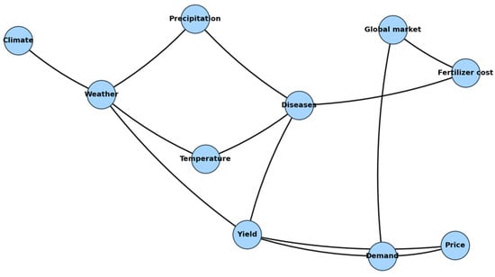
Figure 1. Bayesian network of uncertainties.

• Climate affects weather, weather affects temperature and precipitation.
• Temperature and precipitation together determine the probability of disease occurrence.
• Weather and diseases affect crop yields.
• Yield and the global market shape demand.
• Demand and crop yields determine product prices.
• The global market and diseases affect the cost of fertilizers.

This structure allows us to formally describe the complex, multi-level relationships between all key factors of uncertainty in agricultural production.

Each node in the network is assigned a conditional probability table (CPT). Table 1 shows the probabilities for some key nodes as an example.

Table 1. CPT fragment.

№	Climate	Weather	Temperature	Precipitation	Diseases	Yield	Fertilizer Costs	Global Market	Demand	Price	Probability
1	Stable	Benefit.	Normal	Normal	No	High	Low	Stable	High	High.	0.109610
2	Stable	Good.	Extreme	Normal	No	High	Low	Stable	High	High	0.031317
3	Stable	Good.	Normal	Anom.	No	High	Low	Stable	High	High	0.028417
4	Change	Benefit.	Normal	Normal	No	High	Low	Stable	High	High	0.027402

Probabilities can be obtained based on expert estimates, historical data analysis, and statistical or machine models trained on corporate/industry data. Detailed methods for obtaining CPT are discussed in previous sections of this article.

The Variable Elimination algorithm (implemented in the pgmpy library) is used to derive the probabilities of all possible combinations of system states. This derivation allows us to automatically obtain joint probabilities for all scenarios, even with a large dimension of uncertainty space. Table 2 shows a fragment of the joint probability distribution for the most likely scenarios.

Table 2. Fragment of the joint probability distribution.

№	Probability	Profit_A	Profit_B
1	0.109610	1980.0	1782.0
2	0.031317	1980.0	1782.0
3	0.028417	1980.0	1782.0
4	0.027402	1980.0	1782.0

Using the obtained joint probabilities of scenarios, the corresponding profit from growing crops A and B is calculated for each scenario (taking into account yield, price, demand, and resource costs). The total expected profit for each crop is determined as the weighted sum across all scenarios. The problem is formulated as a linear programming problem:

$${\mathrm{m}\mathrm{a}\mathrm{x}}_{{\mathrm{x}}_{\mathrm{A}},{\mathrm{x}}_{\mathrm{B}}}\hspace{0.25em} ({\mathrm{x}}_{\mathrm{A}}\cdot \mathrm{E}[{\mathrm{P}}_{\mathrm{A}}]+{\mathrm{x}}_{\mathrm{B}}\cdot \mathrm{E}[{\mathrm{P}}_{\mathrm{B}}\left]\right)$$

$${\mathrm{x}}_{\mathrm{A}}+{\mathrm{x}}_{\mathrm{B}}\le {\mathrm{X}}_{\mathrm{m}\mathrm{a}\mathrm{x}}$$

$${\mathrm{x}}_{\mathrm{A}}\ge 0,\hspace{0.25em} \hspace{0.25em} {\mathrm{x}}_{\mathrm{B}}\ge 0\mathrm{ }$$

where

• x_A, x_B—areas sown with crops A and B;
• E[P_A], E[P_B]—expected profits per unit area, calculated according to BN.

In the basic version (without additional constraints), the solution to the problem leads to maximization of the area of the most profitable crop, which leads to a “one-sided” result (the entire field is occupied by the crop with the maximum expected income). This reflects a classic feature of linear models with constraints only on the total resource.

For more realistic and balanced optimization, additional constraints were introduced:

• Resource cost constraint: A limit on the budget for fertilizers and chemicals (e.g., no more than 35,000 currency units for the entire farm).
• Chance constraints (risk management): A requirement that profits in “adverse” scenarios (low yields) exceed a certain minimum.
• Nonlinear effects (e.g., market saturation): A decrease in additional profit when the area of a single crop is increased due to a drop in demand or price.

The optimization results taking these factors into account are shown in Table 3 and Figure 2. As can be seen, as the problem becomes more complex and constraints are added, the solutions become more balanced and economically sustainable, and the area is divided between crops more flexibly.

Table 3. Distribution and expected profit under different conditions.

Method	A	B	Expected Profit
LP + BN (baseline)	10	0	144,787.79
LP + BN + fertilizer restriction	33.92	66.08	135,219.64
LP + BN + chance restrictions	39.27	60.73	135,995.01
LP + BN + market saturation	33.3	50	41,723.82

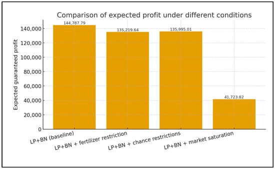
Figure 2. Comparison of expected profits under different conditions.

Table 3 and Figure 2 show the values of optimal profits and space structures for different problem formulations:

The graph (Figure 2) shows how the expected profit and decision structure change when moving from the simplest formulation to the extended one, illustrating the flexibility and adaptability of the method.

5.3. Comparison of the Proposed Approach with Traditional Methods

To compare the effectiveness of the proposed methodology, an analysis was conducted using classical approaches:

• Stochastic programming: Simple probability scenarios were considered without taking into account dependencies (for example, independent probabilities of “weather” and “yield”).
  The result is often overestimated or underestimated profits with a failure to take joint risks into account.
• Robust optimization: Maximization of profits in the worst (most unfavorable) scenario.
  The solution turns out to be too conservative, and potential may not be fully realized.
• Distributed robust optimization (DRO): Accounting for uncertainty in the probabilities of the scenarios themselves (e.g., varying the probability of “favorable weather” within a certain range). The solution is more robust, but requires searching through scenarios and does not take structural dependencies into account.
  The comparison results are presented in Table 4 and Figure 3.
  Table 4. Comparison with classical methods.

  Method	Expected Profit	Nature of the Solution	Complexity of Implementation
  LP + BN (proposed)	135,219.64	Flexible, realistic	Medium
  Stochastic	153,000.00	Usually one-sided	Low
  Robust	110,000.00	Very conservative	Low
  DRO	144,000.00	Moderately conservative	Average

  

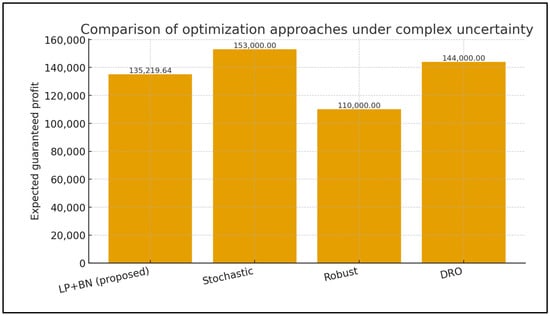  Figure 3. Comparison of optimization approaches under complex uncertainty.

As can be seen, the proposed approach provides more realistic and flexible solutions, especially when there are complex interdependencies between sources of uncertainty. In addition, automating probability inference through BN offers advantages in computational efficiency and adaptability compared to manual scenario exploration.

5.4. Sensitivity to BN Parameters

We quantify how sensitive the BN → LP objective is to small, local changes in the BN parameters. For each CPT column (a fixed parent configuration), we shift a probability mass of δ = 0.05 toward the first state of the child, re-normalize the column, recompute the expected-profit objective, and repeat with a −δ shift. The one-way effect for a column is measured as $\mathrm{m}\mathrm{a}\mathrm{x}\left(\right|\mathsf{\Delta }+|,|\mathsf{\Delta }-\left|\right),$ where $\mathsf{\Delta }\pm$ is the change in the LP optimum under the perturbed BN. We then aggregate to the node level by taking the maximum effect over all columns of the node. The tornado plot reports the top CPT columns ranked by effect; the summary table reports node-level maxima and the same values as a percentage of the baseline objective.

Across all CPT columns, the largest effects come from the yield mechanism. Six yield columns dominate the top of the tornado, with the strongest single-column effect observed for $\mathrm{Y}\mathrm{i}\mathrm{e}\mathrm{l}\mathrm{d}\mid \{\mathrm{D}\mathrm{i}\mathrm{s}\mathrm{e}\mathrm{a}\mathrm{s}\mathrm{e}=\mathrm{N}\mathrm{o},\hspace{0.17em}\mathrm{W}\mathrm{e}\mathrm{a}\mathrm{t}\mathrm{h}\mathrm{e}\mathrm{r}=\mathrm{G}\mathrm{o}\mathrm{o}\mathrm{d}\}$ producing a change of 525.54, equal to 7.12% of the baseline objective. Price columns are next in importance (e.g., $\mathrm{P}\mathrm{r}\mathrm{i}\mathrm{c}\mathrm{e}\mid \mathrm{D}\mathrm{e}\mathrm{m}\mathrm{a}\mathrm{n}\mathrm{d}=\mathrm{H}\mathrm{i}\mathrm{g}\mathrm{h}$ yields 138.00 or 1.87%), followed by Weather and Fertilizer-cost channels whose leading columns contribute effects around 110–110 units (≈1.5%). Disease and Demand have moderate influence (≈0.9%), while upstream exogenous drivers such as GlobalMarket and Climate show smaller but non-negligible leverage (≈0.8% and ≈0.6%). Temperature and Precipitation register only marginal impacts (<0.06%), indicating effective attenuation of their uncertainty by downstream structure before it reaches the LP objective.

Practically, these results locate the highest-leverage places for expert elicitation and data collection. Improving or stress-testing the yield CPTs—especially in good-weather, no-disease regimes—will most reduce model risk in the optimization output. Monitoring or hedging demand-driven price movements is the second priority, followed by keeping fertilizer-cost priors current when disease prevalence is low. Upstream climate variables matter primarily through their propagation to weather and disease, so coarse priors are acceptable unless the application requires extreme-scenario assurance.

Figure 4 reports a one-way CPT sensitivity with a ±δ = 0.05 probability shift and full re-normalization. The largest effects come from the Yield CPT columns conditioned on Weather and Disease: moving probability mass to the ‘High’ yield state under Disease = No, Weather = Good increases the objective by about +526; even under adverse weather the gain remains +286–340. Next in importance are Price|Demand entries (+114–138), then Weather|Climate = Stable (~+110). Fertilizer-cost CPT entries (Low cost under calm or stress markets) contribute +73–110. Disease and Demand themselves are moderate drivers (~64–70), while GlobalMarket and Climate are smaller (~42–62). Temperature and Precipitation have negligible local impact (≈3–4 each). Table 5 aggregates the results at the node level and confirms the ranking: Yield dominates (max |Δ| = 525.54, 7.12% of the baseline objective 7385.92), followed by Price (1.87%), then Weather and FertCost (≈1.5% each). This pattern is consistent with the LP objective: changes that directly alter expected yield and selling price have the strongest leverage, whereas upstream drivers are attenuated through the BN before reaching the objective.

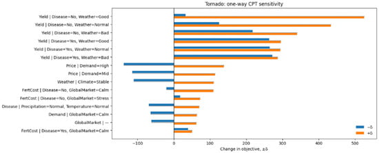
Figure 4. Tornado plot of one-way CPT sensitivity.

Table 5. Node-level sensitivity summary.

Variable	Max Δ Objective	Max Δ Objective, (%)
Yield	525.540	7.115
Price	138.000	1.868
Weather	110.338	1.494
FertCost	109.593	1.484
Disease	69.693	0.944
Demand	64.167	0.869
GlobalMarket	62.122	0.841
Climate	42.240	0.572
Temperature	3.967	0.054
Precipitation	2.847	0.039

5.5. Scalability Mini-Tests

Below we quantify tractability and show two quick stress-tests that mirror the theory in Section 4.7. Exact VE on a BN with $\mathrm{m}$ nodes, maximum state cardinality $r=maxi\mid Si\mid ,$ and (moralized) treewidth $\mathrm{w}$ has time $O(m\hspace{0.17em}{r}^{\hspace{0.17em}w+1})$ and memory $O\left(r^{\hspace{0.17em}w+1}\right).$ CPT storage scales as $\sum _{i=1}^m|S_i\left|\prod _{j\in Pa\left(i\right)}|S_j\right|$. In our pipeline the LP never enumerates scenarios; coefficients are expectations taken over the relevant BN subgraph R induced by the variables that actually enter bindings. End-to-end complexity is therefore End-to-end complexity is therefore T_total as defined in Section 4.7.

We evaluate this on a large public BN (“Link”, 724 nodes, 1125 edges, r = 3). The full model has $w_R=6$ for our targets, giving a proxy $m_R{r}^{w_R+1}=\mathrm{314,928}$. We then apply three dimension-reduction schemes prior to VE: (i) Markov-blanket pruning around the bound variables (blanket), (ii) mutual-information screening within the blanket to keep only the top parents for each target (blanket + MI), and (iii) a light CPT approximation on the reduced model (blanket + MI + approx). For each variant we measure BN wall-time, peak BN memory, LP wall-time, and the resulting objective.

On Link, BN time drops from 7.713 s (full) to 0.451 s (blanket), 0.327 s (blanket + MI), and 0.334 s (blanket + MI + approx), while the objective changes by only −0.00982 in absolute terms (≈−0.005% relative) (Table 6 and Table 7). Peak BN memory falls from 271.5 MB (full) to 0.066 MB (blanket), 0.045 MB (blanket + MI), and 0.049 MB (blanket + MI + approx). The reduced models also shrink the induced width: $w_R$ goes from 6 → 3 → 2 → 2, and the proxy from 314,928 → 891 → 216 → 216. LP time remains at ~1–3 ms across all settings, confirming that BN inference dominates end-to-end runtime. A log–log fit of BN time versus the proxy $m_R{r}^{w_R+1}$ gives a positive slope (≈0.08 on this run), consistent with the theoretical dependence; the single-network slope is not meant as a universal exponent, but it validates the proxy as an explanatory covariate for time.

Table 6. Ablation results.

Variant	Objective Value	BN Wall-Time	BN Peak Memory	LP Wall-Time	LP Peak Memory	Total Wall-Time	BN Nodes	BN Edges	Induced Width	Complexity Proxy	Δ Objective
full	195.603900	7.713398	271.520619	0.002800	0.029552	7.716198	724	1125	6	314,928.0	0.00000
blanket	195.594079	0.450979	0.065834	0.001764	0.008825	0.452743	11	10	3	891.0	0.00982
blanket + MI	195.594079	0.327279	0.044991	0.001358	0.008825	0.328637	8	7	2	216.0	0.00982
blanket + MI + approx	195.594079	0.334039	0.048946	0.002162	0.008825	0.336201	8	7	2	216.0	0.00982

Table 7. Ablation summary.

Variant	Median Speedup	Median Mem Ratio	Median Δobj %
blanket	17.103674	0.000242	−0.005021
blanket + MI	23.568278	0.000166	−0.005021
blanket + MI + approx	23.091295	0.000180	−0.005021
full	1.000000	1.000000	0.000000

Interpretation is straightforward. Time and memory track the induced relevant width $w_R$ as predicted, and simple structural reductions recover one to two orders of magnitude in runtime and three to four orders of magnitude in memory, with sub-basis-point loss in the objective. Markov-blanket pruning brings most of the gain by eliminating nodes that cannot affect the bindings; MI screening removes weak blanket parents with negligible impact on the LP coefficients; the lightweight CPT approximation yields similar accuracy at essentially the same cost. These results indicate that large BNs can be made operational for BN → LP by targeting $\mathrm{R}$ and $w_R$, and that the proxy $m_R{r}^{w_R+1}$ is a useful design dial for engineering tractable models without sacrificing decision quality.

5.6. Dynamic BN → LP

We implement a receding-horizon loop that updates the BN from newly observed signals and resolves the LP at every step. Horizon T = 12. At time t we observe Weather and Demand, compute posteriors for the LP-relevant marginals $\left\{P\right(Yield=High),P(Price=High),P(FertCost=Low\left)\right\},$ convert them to coefficients $c_A\left(p\right),c_B\left(p\right)$ and solve $\max c^{t}x$ subject to $+x_B\le 100,x\ge 0.$ Only the coefficients change over time; the feasible set is fixed.

Figure 5 shows two panels. The upper panel plots the expected profit at each step with the observed pair (Weather, Demand) annotated. The lower panel shows the resulting allocations $x_A$ and $x_B$. Table 8 lists the same sequence numerically.

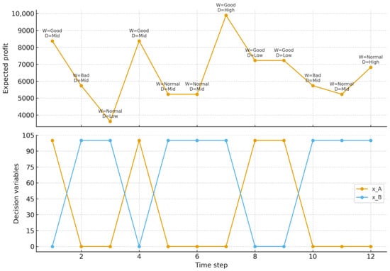
Figure 5. Profit and allocations.

Table 8. Step-by-step observations and decisions.

t	xA	xB	Expected Profit	Observed Weather	Observed Demand
1	100.0	0.0	8378.002363	Good	Mid
2	0.0	100.0	5733.746184	Bad	Mid
3	0.0	100.0	3626.348438	Normal	Low
4	100.0	0.0	8378.002363	Good	Mid
5	0.0	100.0	5228.189803	Normal	Mid
6	0.0	100.0	5228.189803	Normal	Mid
7	0.0	100.0	9891.706217	Good	High
8	100.0	0.0	7224.465975	Good	Low
9	100.0	0.0	7224.465975	Good	Low
10	0.0	100.0	5733.746184	Bad	Mid
11	0.0	100.0	5228.189803	Normal	Mid
12	0.0	100.0	6822.651359	Normal	High

The policy reacts sharply to information, which is expected with a linear objective and a single resource constraint. Good weather with mid demand drives $x_A=100\%$ and profit around $8.38\times 10^3$ (steps 1 and 4). Good weather with high demand shifts to $x_B=100\%$ and yields the peak $9.89\times 10^3$ (step 7). Bad weather or normal-low demand tilt the coefficients toward crop B, producing $x_B=100\%$ and lower profits in the $3.63-5.73\times 10^3$ range (steps 2–3, 5–6, 9–11). Good-low cases still favor A at $7.22\times 10^3$ (steps 8–9). Over the full horizon, the mean profit is $6.56\times 10^3$, the minimum is $3.63\times 10^3$, and the maximum is $9.89\times 10^3$. Corner solutions dominate: $x_A=100\%$ in one-third of the steps and $x_B=100\%$ in two-thirds, which is consistent with linear programming under changing coefficients.

These results illustrate an MPC-style operation: BN inference converts streaming evidence into posterior scenario weights; the LP instantly recomputes the optimal action under the updated expectations. The closed loop is stable in the sense that allocations switch only when the observed pair (Weather, Demand) crosses intuitive thresholds that alter the relative expected margins of crops A and B.

6. Discussion

The main innovation is the end-to-end integration of Bayesian networks (BN) and linear programming (LP) to optimize solutions with multiple causally related sources of uncertainty. Unlike classical stochastic and robust schemes (including DRO), which rely on manual scenario search, parameter independence, or “flat” uncertainty sets, here, event probabilities are included in the optimization through posterior BN and directly determine LP coefficients. This provides reproducible risk calibration and a clear distinction between “possible” and “probable”: risk is controlled by chance constraints or small sets of ambiguity around the posterior BN, which removes the excessive conservatism of flat RO with a comparable level of guarantees and without the internal minimax search characteristic of DRO.

As shown in the examples, BN formalizes the hierarchy of risk factors—climate, weather, disease, market, and costs—and allows for the calculation of joint probabilities of scenarios, taking into account causal relationships. Key point: LP does not require listing scenarios. The coefficients of the objective and constraints are extracted from the marginal distributions on the relevant subgraph of the ancestors of the variables included in the formulation. Thus, the computational complexity is localized not “to the entire graph,” but to the induced width of this particular subgraph; theoretically, this is formalized in the section on complexity and empirically confirmed by scalability curves (acceleration from Markov-blanket truncation, selection of weak parents based on mutual information, and structured/low-rank CPDs without noticeable loss in the objective function).

The practical value is especially great where uncertainty is multifactorial and structurally related. In such problems, independent scenarios overestimate the nominal benefit and underestimate joint tails, while BN → LP maintains the specified level of risk and provides more realistic solutions. Conversely, with a small number of truly independent random parameters, the advantages are minimal: solutions converge to the results of classical approaches, and model complexity is not necessary.

The limitations are transparent. Data quality for the structure and CPT is critical: unstable expert estimates or sparse statistics worsen the posterior and, as a result, the LP coefficients. This risk is partially mitigated by a standardized network construction process: narrowing the space of structures, reconciling data and expertise through Dirichlet smoothing (pseudo-counts as priors), and subsequent sensitivity. In the sensitivity method, CPT columns are varied with full renormalization, the change is passed through the BN, and the LP is recalculated; aggregated tornado diagrams by nodes show which parameters contribute most to the target response, i.e., where it is rational to spend effort on data collection or re-elicit.

From a computational point of view, the bottleneck is the inference in BN, not the LP solution. Thanks to localization on the ancestor subgraph and the use of VE/belief messages, the computations remain manageable for moderate graph widths, and for large applications, engineering techniques are available: structured CPDs (e.g., Noisy-OR/log–linear forms) to reduce parameters, parent selection based on mutual information for LP-relevant goals, state clustering, and approximate/variational inference. Time and memory metrics correlate well with proxies based on induced width, confirming cost predictability and providing a practical “ruler” for designing networks under computational platform constraints.

Dynamic scenarios are naturally supported through the “DBN → posterior update → LP coefficient recalculation → new solution” loop. Since the feasible set is usually fixed, only the coefficients change, and caching of order of exception and factors makes online updates significantly cheaper than a complete rebuild. This ensures adaptability and stability when new data arrives without resorting to heavy two-level formulations.

Taken together, the results show that when structural complexity is high, replacing “flat” sets with posterior probabilities and translating causal knowledge into LP coefficients improves risk control and decision quality at an acceptable computational cost; when the structure is simple, the gains are small and traditional means are sufficient.

7. Conclusions

This paper develops and analyzes a general method for integrating Bayesian networks with linear programming to solve optimization problems under complex, multidimensional, and structured uncertainty. The main contribution is a unified formal scheme that maps BN posteriors onto LP coefficients, thereby preserving causal dependencies among uncertain parameters typical of real production, economic, and management tasks. Probability enters the optimization in a calibrated and reproducible way, rather than through manually specified or independence-based scenarios.

The agro-industrial case study demonstrates practical feasibility and decision quality. Under matched risk control, the BN → LP pipeline maintains the target violation rate while avoiding the over-conservatism of flat robust optimization and the optimism of independence-based stochastic programming; at the same time it circumvents the inner min–max machinery common in distributionally robust optimization (DRO). Posterior weighting explicitly demarcates what is feasible from what is probable, so extreme yet implausible cases influence the decision in proportion to their credibility. This separation is essential when many drivers interact and tail events arise from causal propagation across weather, disease, yield, demand, prices, and input costs.

The approach avoids explicit scenario enumeration; computational cost is governed by BN inference over the decision-relevant ancestor subgraph that populates the LP objective and bindings. Empirical scaling curves indicate that wall-time and memory correlate with the induced width of this subgraph, and that Markov-blanket pruning, mutual-information screening of weak parents for LP-relevant targets, and structured or low-rank CPDs deliver substantial savings with negligible impact on the objective. The largest gains arise when uncertainty is high-dimensional and structurally coupled. When uncertainty is low-dimensional and essentially independent, BN → LP tends to recover the allocations of classical methods and offers limited advantage. In practice, feasibility is strongest for problems whose BN-relevant subgraph has moderate induced width, with further scalability enabled by the reduction techniques above.

The practical significance follows from a standardized construction procedure that reconciles data and expertise. Structure learning is constrained and regularized; CPTs are updated by Dirichlet smoothing that treats expert inputs as pseudo-counts; and a systematic sensitivity analysis quantifies how perturbations in CPT columns propagate to the LP objective, identifying where targeted data collection or refined elicitation has the highest value. A receding-horizon DBN → LP loop shows how the same pipeline supports dynamic operation: new evidence updates posteriors, coefficients are refreshed, and the LP is re-solved while the feasible set remains fixed, enabling adaptive control without intractable bilevel formulations.

Further development includes automated structure learning constrained by expert priors, online CPT updates from streaming data, and rigorous calibration of Dirichlet strength and DRO ambiguity radii to meet target risk levels. Extending the pipeline to multi-stage settings via dynamic Bayesian networks and advancing scalable inference through variational or selective methods remain priorities for large industrial instances.

Overall, the BN → LP framework provides a coherent and practical route to risk-aware optimization under structured uncertainty and can serve as a foundation for adaptive decision-support systems in data-rich industrial settings.

References

- Keith, A.J.; Ahner, D.K. A survey of decision making and optimization under uncertainty. Ann. Oper. Res. 2021, 300, 319–353. [Google Scholar] [CrossRef]
- Shariatmadar, K.; Wang, K.; Hubbard, C.R.; Hallez, H.; Moens, D. An introduction to optimization under uncertainty—A short survey. arXiv 2022, arXiv:2212.00862. [Google Scholar]
- Li, C.; Grossmann, I.E. A review of stochastic programming methods for optimization of process systems under uncertainty. Front. Chem. Eng. 2021, 2, 622241. [Google Scholar] [CrossRef]
- Sun, X.A.; Conejo, A.J. Robust Optimization in Electric Energy Systems; Springer: Cham, Switzerland, 2021; p. 313. [Google Scholar] [CrossRef]
- Rahimian, H.; Mehrotra, S. Frameworks and results in distributionally robust optimization. Open J. Math. Optim. 2022, 3, 1–85. [Google Scholar] [CrossRef]
- Kuhn, D.; Shafiee, S.; Wiesemann, W. Distributionally robust optimization. Acta Numer. 2025, 34, 579–804. [Google Scholar] [CrossRef]
- Nie, J.; Yang, L.; Zhong, S.; Zhou, G. Distributionally robust optimization with moment ambiguity sets. J. Sci. Comput. 2023, 94, 12. [Google Scholar] [CrossRef]
- Wang, Z.; Jiang, S.; Lin, Y.; Tao, Y.; Chen, C. A review of algorithms for distributionally robust optimization using statistical distances. J. Ind. Manag. Optim. 2024, 21, 1749–1770. [Google Scholar] [CrossRef]
- Ghahtarani, A.; Saif, A.; Ghasemi, A. Robust portfolio selection problems: A comprehensive review. Oper. Res. 2022, 22, 3203–3264. [Google Scholar] [CrossRef]
- Mukhopadhaya, J.; Whitehead, B.T.; Quindlen, J.F.; Alonso, J.J.; Cary, A.W. Multi-fidelity modeling of probabilistic aerodynamic databases for use in aerospace engineering. Int. J. Uncertain. Quantif. 2020, 10, 425–447. [Google Scholar] [CrossRef]
- Mishra, A.A.; Mukhopadhaya, J.; Iaccarino, G.; Alonso, J. Uncertainty estimation module for turbulence model predictions in SU2. AIAA J. 2019, 57, 1066–1077. [Google Scholar] [CrossRef]
- Khodakarami, V. Applying Bayesian Networks to Model Uncertainty in Project Scheduling. Ph.D. Thesis, Queen Mary University of London, London, UK, 2009. [Google Scholar]
- Zheng, H.; Xie, W.; Ryzhov, I.O.; Xie, D. Policy optimization in dynamic Bayesian network hybrid models of biomanufacturing processes. INFORMS J. Comput. 2023, 35, 66–82. [Google Scholar] [CrossRef]
- Iseri, F.; Iseri, H.; Shah, H.; Iakovou, E.; Pistikopoulos, E.N. Planning strategies in the energy sector: Integrating Bayesian neural networks and uncertainty quantification in scenario analysis & optimization. Comput. Chem. Eng. 2025, 198, 109097. [Google Scholar] [CrossRef] [PubMed]
- Ding, C.; Dang, C.; Broggi, M.; Beer, M. Estimation of Response Expectation Bounds under Parametric P-Boxes by Combining Bayesian Global Optimization with Unscented Transform. ASCE-ASME J. Risk Uncertain. Eng. Syst. Part A Civ. Eng. 2024, 10, 04024017. [Google Scholar] [CrossRef]
- Guillaume, R.; Kasperski, A.; Zieliński, P. Distributionally robust possibilistic optimization problems. Fuzzy Sets Syst. 2023, 454, 56–73. [Google Scholar] [CrossRef]
- Gray, A.; Wimbush, A.; De Angelis, M.; Hristov, P.O.; Miralles-Dolz, E.; Calleja, D.; Rocchetta, R. Bayesian calibration and probability bounds analysis solution to the Nasa 2020 UQ challenge on optimization under uncertainty. In Proceedings of the 29th European Safety and Reliability Conference (ESREL), Venice, Italy, 1–5 November 2020; pp. 1111–1118, Research Publishing Services. [Google Scholar] [CrossRef]
- Insua, D.R.; Criado, R. Topics on the foundations of robust Bayesian analysis. Robust Bayesian Anal. 2000, 10, 33–44. [Google Scholar] [CrossRef]
Disclaimer/Publisher’s Note: The statements, opinions and data contained in all publications are solely those of the individual author(s) and contributor(s) and not of MDPI and/or the editor(s). MDPI and/or the editor(s) disclaim responsibility for any injury to people or property resulting from any ideas, methods, instructions or products referred to in the content. |
© 2025 by the authors. Licensee MDPI, Basel, Switzerland. This article is an open access article distributed under the terms and conditions of the Creative Commons Attribution (CC BY) license (https://creativecommons.org/licenses/by/4.0/).