Article

CQEformer: A Causal and Query-Enhanced Transformer Variant for Time-Series Forecasting

School of Mathematics, Physics and Statistics, Shanghai University of Engineering Science, Shanghai 201620, China
*
Author to whom correspondence should be addressed.
Mathematics 2025, 13(23), 3750; https://doi.org/10.3390/math13233750 (registering DOI)
Submission received: 22 October 2025 / Revised: 9 November 2025 / Accepted: 20 November 2025 / Published: 22 November 2025

Abstract

Structural breaks and volatility clustering are fundamental challenges in time series analysis. We propose CQEformer, an encoder-only Transformer variant for time-series modeling that addresses these challenges via two complementary innovations. First, the causal residual embedding (CRE) ensures temporal causality and improves local adaptivity to abrupt structural changes. Second, the query-enhanced multi-head self-attention (QEAttention) incorporates multi-order moment statistics and entropy to guide attention dynamically toward high-volatility regions while preserving global dependence structures. For parameter optimization, we derive analytical gradients for all components and update them using the Adam stochastic optimization algorithm. Empirical evaluations on financial time series datasets and the public Traffic dataset show that CQEformer consistently outperforms established baselines, including LSTM, GRU, TCN, and the standard Transformer. Time-window sensitivity analyses demonstrate the robustness of the framework, while ablation studies further confirm that the proposed modules are complementary and contribute to improved forecasting performance across different volatility regimes.

1. Introduction

Time series arising in complex systems, such as financial markets, exhibit key statistical properties in asset price time series, including volatility clustering, heteroskedasticity, periodicity, and nonstationarity [1]. These characteristics increase the difficulty of accurate modeling and forecasting, which is critical in practical scenarios such as high-frequency trading, quantitative stock selection, and asset allocation.
Traditional approaches, including Autoregressive Integrated Moving Average [2], Vector Autoregression [3], and Generalized Autoregressive Conditional Heteroskedasticity [4], offer interpretability and theoretical completeness and can model linear correlations and conditional heteroskedasticity to some extent. However, they fail to adequately model nonlinear and high-dimensional dependencies in financial markets and lack robustness due to sensitivity to specification, distributional assumptions, and regime shifts [5,6,7].
Deep learning methods have demonstrated strong capabilities in capturing nonlinear patterns and high-dimensional representations. Recurrent architectures such as Recurrent Neural Network (RNN), Long Short-Term Memory network (LSTM), Gated Recurrent Unit (GRU), and their variants have been applied to stock price forecasting. For instance, Nguyen et al. [8] proposed the SR-SV model, combining RNN with stochastic volatility models (SV), achieving strong out-of-sample predictive performance and interpretability. Sang and Li [9] enhanced LSTM structures with attention mechanisms in AMV-LSTM, improving stability and predictive accuracy, while Ming-Che Lee integrated GRU with attention to predict significant price fluctuations [10]. Nevertheless, these methods face limitations in modeling long-term dependencies and enabling efficient parallel training.
The introduction of the Transformer architecture has provided a promising alternative [11]. Its self-attention mechanism excels at capturing long-range dependencies and has inspired variants such as Informer [12], FEDformer [13], PatchTST [14], TimesNet [15], iTransformer [16], Pathformer [17], Twinsformer [18], and Timer-XL [19], demonstrating strong performance in general-purpose time series forecasting. Yet these models do not fully account for financial data’s unique properties, such as local anomalies, tail risks, and volatility clustering.
To address these domain-specific challenges, some works have customized Transformer architectures for financial applications. Ding et al. [20] proposed a Transformer enhanced with multi-scale Gaussian priors, orthogonal regularization, and a trading-gap segmenter, achieving strong results on NASDAQ and Chinese A-share markets. Zhang et al. [21] combined refined small-sample feature engineering with multiple attention mechanisms, attaining high predictive accuracy and improved realized returns. Nonetheless, domain-specific Transformer variants remain limited and lack systematic development, and as a result, leaving complex statistical characteristics and risk features underexploited.
To confront the key challenges of financial time series prediction—dynamic volatility, structural breaks, and nonstationarity—we propose CQEformer, an Encoder-Only Transformer variant that integrates Causal Convolution Residual Embedding with a Statistical-Prior-Enhanced Query Mechanism. This architecture is specifically designed to capture both local temporal patterns and global structural dynamics in complex, high-noise financial data, with two core innovations detailed as follows:
  • Causal convolutional residual embedding in the input layer, emphasizing spatiotemporal locality and enforcing temporal causality. By focusing on residual features between consecutive time steps, the model improves sensitivity to sudden market shocks, structural breaks, and local anomalies, thereby enhancing short-term predictive accuracy and stability.
  • Query-Enhanced multi-head self-attention mechanism, dynamically adjusting the Query matrix using higher-order statistical moments and entropy in time and frequency domains. This guides attention to regions exhibiting volatility clustering and sudden structural shifts, improving modeling of tail risks and nonlinear market behaviors.
Unlike recent frequency-aware or decomposition-based Transformers, CQEformer explicitly combines CRE for local temporal patterns with QEAttention, which injects multi-order time– and frequency–domain priors into attention logits. This design enables more effective amplification of tail and high-volatility signals and facilitates capturing both local and global dynamics, complementing existing approaches.
In Section 4, we provide comprehensive evaluations, including multi-model comparison across three real-world datasets and further analyses—time-window sensitivity and ablation studies—conducted on the CSI 300 dataset. The results show that CQEformer consistently outperforms baseline models, effectively captures complex temporal dynamics, and maintains robustness across varying market conditions.

2. Background

2.1. Problem Setup

Consider the problem of time series forecasting: Given a multivariate time series X R L × D , where L denotes the number of time steps and D is the feature dimension. Let y R L denote the target label, the objective is to learn a mapping f: R L × D R L to predict the future values y ^ R L over the next L steps, as follows:
y ^ = f ( X ) .

2.2. Encoder-Only Transformer

An encoder-only Transformer typically consists of four main components: an input embedding layer that maps raw features to a high-dimensional space, positional encoding to inject sequence order information, a stack of encoder layers—each containing multi-head self-attention (MSA) and feed-forward network (FFN) with residual connections (Res) and layer normalization (LayerNorm)—to extract contextual representations, and an output layer to produce the final predictions. The architecture is shown in Figure 1.
  • Input Embedding and Positional Encoding
For a standardized multivariate time series X R L × D , it is first projected into a high-dimensional space R L × H , where H is the embedding dimension. The standard Transformer applies a fully connected layer to obtain X e , and then
X e = X · W e + 1 L · b e T ,
where W e R D × H , b e R H are learnable, 1 L denotes a L-dimensional all-ones vector. The Transformer is permutation-equivariant and cannot capture order [22], a positional encoding PE R L × H is therefore introduced, with elements defined as
PE i j = sin i 1 10000 j 1 H , j = 2 k 1 , cos i 1 10000 j 1 H , j = 2 k ,
where i = 1 , 2 , , L , k = 1 , 2 , , H / 2 . Then PE is added to the X e to obtain X i n ,
X i n = X e + PE .
  • Multi-Head Self-Attention
MSA ( · ) is defined as the multi-head self-attention, calculated as follows. With N heads (H divisible by N), let S = H / N denote head’s dimension, this layer input X i n is mapped into N sets of query, key, and value matrices ( Q i , K i , V i ) , i = 1 , 2 , , N ,
Q i = X i n · W Q i + 1 L · b Q i , K i = X i n · W K i + 1 L · b K i , V i = X i n · W V i + 1 L · b V i ,
where W Q i , W K i , W V i R H × S , b Q i , b K i , b V i R S . The attention for one head is computed as
Head i = Attention Q i , K i , V i : = Softmax Q i · K i T S · V i ,
where Softmax is applied row-wise, so that the elements of each row sum to 1. Let Head = Concat Head 1 , Head 2 , , Head N R L × H , the multi-head self-attention is computed as
X m s a = Head · W o + 1 L · b o T ,
where W o R H × H , and  b o R H .
  • First Res & LayerNorm
After multi-head self-attention, a residual connection and a layer normalization are applied, Let μ l n and σ l n denote the row-wise mean and standard deviation, and the normalized output is X l n ,
X r e = Res ( X i n , MSA ) : = X i n + MSA ( X i n ) .
X l n = LayerNorm ( X r e ) : = 1 L · γ l n X r e μ l n · 1 H T σ l n · 1 H T + 1 L · β l n ,
where MSA ( X i n ) = X m s a , γ l n , β l n R H are learnable, ∘ and ⊘ denote element-wise multiplication and division.
  • Feed-Forward Network
D f denotes this network’s hidden dimension, calculation follows:
X f = FFN ( X l n ) : = ReLU X l n · W f 1 + 1 L · b f 1 T · W f 2 + 1 L · b f 2 T ,
where W f 1 R H × D f , W f 2 R D f × H , b f 1 R D f , b f 2 R H .
  • Second Res & LayerNorm
Residual connection and layer normalization are applied again on X l n as in Equations (8) and (9), yielding X e n ,
X e n = LayerNorm ( X l n + X f ) ,
and this LayerNorm contains two learnable parameters γ e n , β e n R H .
  • Output Layer
y ^ = W y · x L + b y ,
where x L denotes the transpose of the L-th row vector of X e n , W y R L × H , b y R L .

3. CQEformer (Causal Query-Enhanced Transformer)

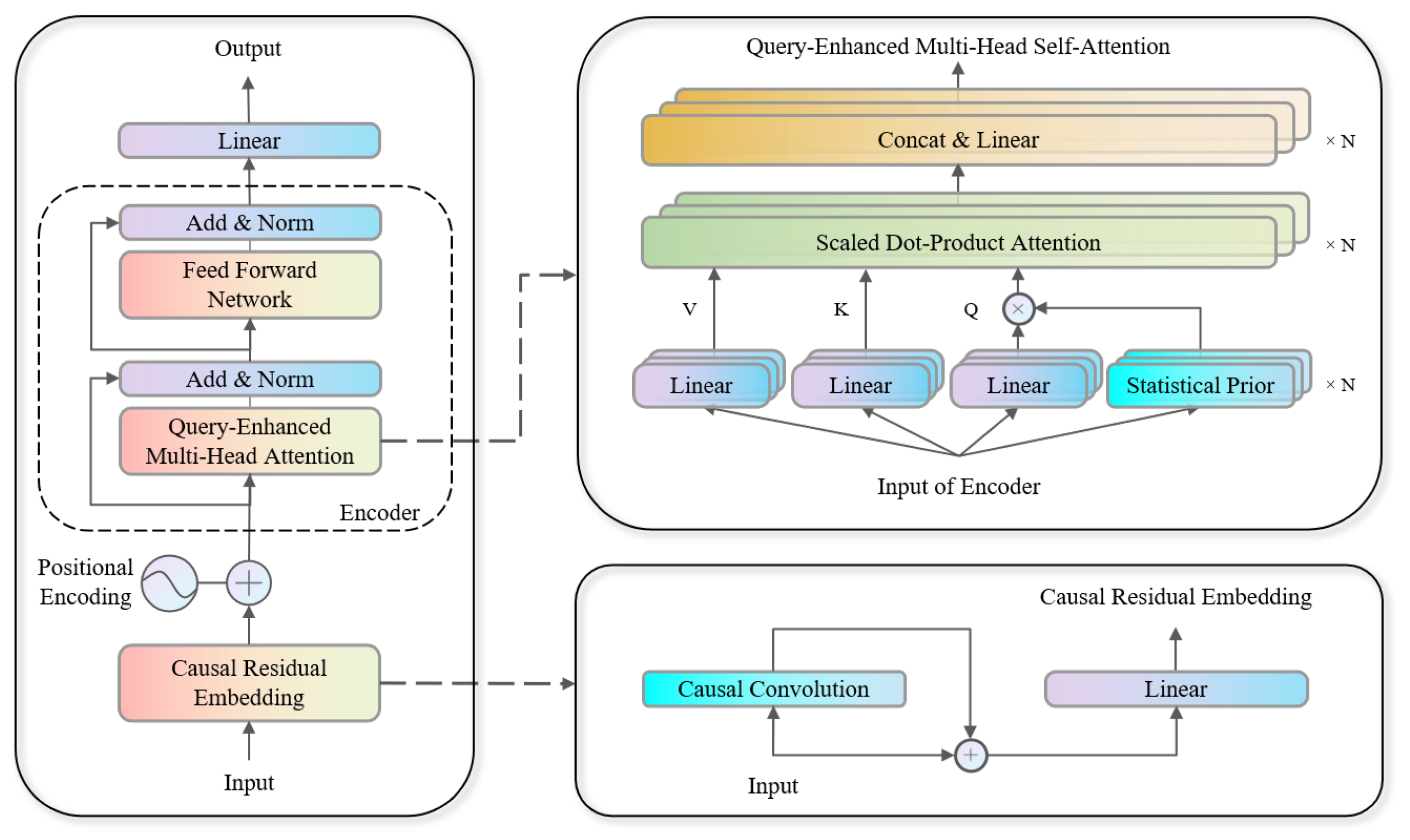
Time series with rapidly changing volatility and structural shifts pose challenges for standard Transformers. To address this, we propose CQEformer, which integrates a causal residual embedding (CRE) module and query-enhanced multi-Head self-attention (QEAttention) mechanism—a novel Attention that injects multi-order time- and frequency–domain priors into attention to focus on high-volatility regimes. CQEformer’s architecture is shown in Figure 2.

3.1. Causal Residual Embedding

We introduce a causal convolutional residual embedding in the input layer, which leverages residual connections with causal convolutions. This design preserves temporal causality and local spatio-temporal structure, enabling the model to capture local fluctuations and respond to sudden shocks. By combining convolutional feature extraction with residual pathways, the embedding remains robust to abrupt changes while retaining the original sequence information.
Causal convolution was introduced in WaveNet to ensure temporal causality in audio modeling [23]. For a standardized multivariate time series X , we define C = CausalConv ( X ) , where CausalConv denotes a causal convolution, each element C i j is computed as follows:
C i j = d = 1 D k = 1 K I i k + 1 0 · X i , d · W c k , d , j + b c j ,
where K is the size of the causal convolution kernel, K N + , I is the indicator function, i = max ( 0 , i k + 1 ) , W c R K × D × H , b c R H . In our experiments, we adopt a small kernel size K = 3 to capture local abrupt changes while maintaining a certain temporal context, which yields the best performance among tested values K = 3 , 5 , 7 , 9 , 11 .
An efficient module, residual connection, was first proposed in ResNet [24], and have been widely adopted. Based on this two structures, we propose causal convolution residual embedding, defined as follows:
X e = ( X + CausalConv ( X ) ) · W e + 1 L · b e T ,
where W e R D × H , b e R H .

3.2. Query-Enhanced Multi-Head Self-Attention Mechanism

Traditional Transformer models struggle to capture volatility that changes rapidly across the entire sequence. To address this, we propose QEAttention, a query-enhanced multi-head self-attention mechanism that projects multi-order statistical moments and entropy from time and frequency domains into head space and uses them as scaling to dynamically reshape attention logits—effectively amplifying and propagating volatility signals across the full attention map, improving model’s ability to capture risk and extreme events.
Given the input matrix X i n , we first compute statistical prior information, including multi-order moments and entropy features in both the time and frequency domains. These features are then used by the QEAttention mechanism to obtain the attention scores.
The time-domain statistics comprise the first-order raw moment μ t , the second-order central moment σ t , the normalized third-order central moment τ t , and the entropy ϵ t , which is computed from its probability matrices P t , via a feature-wise Softmax, as follows,
P t = Softmax ( X i n ) ,
so, these statistics are calculated as follows:
μ t = 1 H X i n · 1 H ,
σ t = 1 H X i n μ t · 1 H T 2 · 1 H 0.5 ,
τ t = 1 H X i n μ t · 1 H T σ t · 1 H T 3 · 1 H ,
ϵ t = P t log P t · 1 H ,
where i denotes the element-wise i-th power.
The frequency–domain statistics—namely the first-order raw moments μ s , the second-order central moments σ s , the normalized third-order central moments τ s , and entropy ϵ s —are computed from the power spectral density (PSD) of the input, which is obtained by applying the Fast Fourier Transform (FFT) along the temporal dimension and taking the squared magnitude of the resulting complex coefficients. Specifically, for  X i n R L × H , we compute
X i n = FFT ( X i n ) : = Ω · X i n , Ω kj = exp 2 π i · ( k 1 ) ( j 1 ) L ,
where k = 1 , , L indexes the frequency components, and  j = 1 , , L indexes the time steps. And we compute PSD as follows:
X p s = | X i n | 2 ,
where | · | denotes element-wise modulus.
From X p s , we derive frequency–domain statistics μ s , σ s , τ s , ϵ s . ϵ s is computed using the probability matrix P s , which is obtained via L1 normalization to preserve energy distribution, as follows:
P s = X p s X p s 1 , row · 1 H T ,
where X p s 1 , row denotes the vector of row-wise L1 norms of X p s .
The frequency–domain statistics of X i n are then calculated as described follows:
μ s = 1 H X p s · 1 H ,
σ s = 1 H X p s μ s · 1 H T 2 · 1 H 0.5 ,
τ s = 1 H X p s μ s · 1 H T σ s · 1 H T 3 · 1 H ,
ϵ s = P s log P s · 1 H .
Next, we concatenate the statistics along the feature dimension and apply LayerNorm to obtain the statistical prior matrix Π :
Π = LayerNorm Concat μ t , σ t , τ t , ϵ t , μ s , σ s , τ s , ϵ s ,
and this LayerNorm contains two learnable parameters γ Π , β Π R 8 . Then, we project Π into head space and apply Tanh to get the statistical prior weight matrix Ψ :
Ψ = Tan h Π · W Ψ + 1 L · b Ψ T ,
where W Ψ R 8 × N , b Ψ R N . X i n is projected into N sets of query, key, and value matrices ( Q i , K i , V i ) , as defined in Equation (5), containing learnable W Q i , W K i , W V i , b Q i , b K i , b V i . The QEAttention for head i produces Head i R L × S , as follows:
Head i = QEAttention Ψ i , Q i , K i , V i : = Softmax Ψ i · 1 S T Q i · K i T S · V i ,
where Ψ i represents the i-th column vector of Ψ .
Finally, let Head = Concat Head 1 , Head 2 , , Head N , and the query-enhanced multi-head self-attention is completed through a linear transformation (containing learnable W o R H × H , b o R H ) in the same way as described in Equation (7), yielding X m s a .

3.3. Forward Propagation Algorithm

After introducing the two improvements, the complete forward propagation algorithm of CQEformer is summarized in Algorithm 1.

3.4. Parameter Optimization

This section details the parameter optimization process of CQEformer during training. We first derive the gradients for all CQEformer modules. Then, we present the parameter update scheme based on the Adam optimizer.

3.4.1. Gradient Derivation

In traditional encoder-only Transformer for time series forecasting (with a single encoder), there are 14 + 6 N learnable parameter groups (N denotes the number of attention heads), each represented by a vector or matrix. These include weight matrices in the set W e , W Q i , W K i , W V i , W o , W f 1 , W f 2 , W y | i = 1 , 2 , , N , bias vectors in the set b e , b Q i , b K i , b V i , b o , b f 1 , b f 2 , b y | i = 1 , 2 , , N and four vectors γ l n , γ e n , β l n , β e n . For CQEformer, a total of 20 + 6 N parameter groups must be updated, which includes the six additional W c , W Ψ , b c , b Ψ , γ Π , β Π from the CRE and QEAttention modules.
Algorithm 1 CQEformer Forecasting Procedure
  • Require: Time series X R L × H , forecast horizon L , model dimension H, encoder numbers E, head numbers N
  • Ensure: Forecast y ^ R L
1:
Step 1: Input Layer
X i n = X + CausalConv ( X ) · W e + 1 L · b e T + PE
2:
Step 2: CQEformer Encoder Layer
3:
for each encoder layer ( i = 1 , , E )  do
4:
    Compute statistical prior information Π :
Π = LayerNorm Concat μ t , σ t , τ t , ϵ t , μ s , σ s , τ s , ϵ s R L × 8
5:
    Compute statistical prior weight matrix Ψ :
Ψ = Tan h Π · W Ψ + 1 L · b Ψ T
6:
    Compute QEAttention mechanism:
7:
    for each head ( i = 1 , , N )  do
Q i = X i n · W Q i + 1 L · b Q i T , K i = X i n · W K i + 1 L · b K i T , V i = X i n · W V i + 1 L · b V i T ,
Head i = Softmax Ψ i · 1 S T Q i · K i T S · V i
X m s a = Concat Head 1 , Head 2 , , Head N · W o + 1 L · b o T
8:
    end for
9:
    Apply first residual connection and layer normalization:
X l n = LayerNorm X i n + X m s a
10:
    Apply feedforward network, second residual connection and layer normalization:
X e n = LayerNorm X l n + FFN X l n
11:
end for
12:
Step 3: Output Layer
y ^ = W y · x L + b y
13:
return  y ^
The Mean Squared Error (MSE) is used as the loss function, as Equation (30). For any parameter X , let δ X represent the gradient of L ( y , y ^ ) with respect to X . Then δ y ^ can be computed as Equation (31):
L ( y , y ^ ) = 1 L y y ^ 2 2 ,
δ y ^ = 2 L ( y y ^ ) .
In output layer, δ W y , δ b y and δ X e n need to be computed as follows:
δ W y = δ y ^ · x y T , δ b y = δ y ^ , δ X e n = 0 ; 0 ; ; 0 ; δ y ^ T · W y .
There are 12 learnable parameter groups in a single encoder. First, we present the derivation of gradients for a general LayerNorm. For  X R L × H , let Y = LayerNorm ( X ) , we define centering operator M = I 1 H 1 H · 1 H T ( I is the identity matrix) and normalized matrix X ˜ = ( X · M ) ( σ · 1 H T ) . These gradients in LayerNorm are given as follows:
δ γ = 1 L T · ( δ Y X ˜ ) , δ β = 1 L T · δ Y , δ X = δ Y ( 1 L · γ ) ( σ · 1 ) L · M .
Using the method outlined in Equation (33), for the backpropagation of second Res & LayerNorm, we can obtain δ γ e n , δ β e n and δ Z , where Z = X l n + FFN ( X l n ) . Additional gradients δ W f 1 , δ W f 2 , δ b f 1 , δ b f 2 and δ X l n can be computed as follows:
δ W f 1 = X l n T · δ Z · W f 2 T I ( T > 0 ) , δ b f 1 = δ Z T · W f 2 T I ( T > 0 ) T · 1 L , δ W f 2 = ReLU ( T ) T · δ Z , δ b f 2 = δ Z T · 1 L , δ X l n = δ Z + δ Z · W f 1 T ,
where T = X l n · W f 1 + 1 L · b f 1 T and I ( T > 0 ) denotes a matrix of the same size as T , where each element is 1 when T i j > 0 , and 0 otherwise. Similarly, we can also obtain the gradients δ γ l n , δ β l n , δ X m s a and δ X i n ( l n ) in first Res & LayerNorm, among which δ X i n ( l n ) denotes a part of the gradient of the loss with respect to X i n that originates from the LayerNorm.
Next, the computation methods of the gradients in QEAttention will be provided. The gradients in the final linear transformation therein are computed as follows:
δ W o = Head T · δ X m s a , δ b o = δ X m s a T · 1 L , δ Head = δ X m s a · W o T ,
and we can further obtain δ Head i since δ Head = Concat ( δ Head 1 , δ Head 2 , , δ Head N ) .
For Equation (29), let T i = Ψ i · 1 S T Q i · ( K i ) T and A = Softmax ( T i S ) , we can compute δ T i = T i S A δ Head i · ( V i ) T A ( δ Head i · ( V i ) T ) · 1 S · 1 S T , and then we can compute the following:
δ Q i = ( δ T i · K i ) ( Ψ i · 1 S T ) , δ K i = δ T i T · ( δ T i · K i ) , δ V i = A · δ Head i , δ Ψ i = ( δ T i · K i ) Q i · 1 S ,
further we obtain δ Ψ = ( δ Ψ 1 , δ Ψ 2 , , δ Ψ N ) . Thus, δ W Ψ , δ b Ψ , δ Π can be computed as follows:
δ W Ψ = Π T · 1 L · 1 H T Ψ 2 δ Ψ , δ b Ψ = 1 L · 1 H T Ψ 2 δ Ψ T · 1 L , δ Π = 1 L · 1 H T Ψ 2 δ Ψ · W Ψ T ,
δ γ Π , δ β Π , δ Λ can be computed based on δ Π using the method as Equation (33), where Λ = μ t , σ t , τ t , ϵ t , μ s , σ s , τ s , ϵ s , and then δ μ t , δ σ t , δ τ t , δ ϵ t , δ μ s , δ σ s , δ τ s , δ ϵ s can be obtained.
Let δ X i n ( q k v ) denote the partial gradients of X i n that originate from the generation process of Q i , K i , V i . Next, we present the form of the gradients in the generation process of Q i , K i , V i , as follows:
δ W Q i = X i n T · δ Q i , δ b Q i = δ Q i T · 1 L , δ W K i = X i n T · δ K i , δ b K i = δ K i T · 1 L , δ W V i = X i n T · δ V i , δ b V i = δ V i T · 1 L ,
δ X i n ( q k v ) = i = 1 N ( δ W Q i · W Q i T + δ W K i · W K i T + δ W V i · W V i T ) .
To obtain the gradients of the last four parameter groups W c , W e , b c , b e whose gradients originate from the loss with respect to the encoder’s input X i n , we first need to compute δ X i n that integrates δ X i n ( l n ) , δ X i n ( q k v ) , and  δ X i n ( Λ ) ; the latter refers to the partial gradients of X i n originating from the generation process of Λ . To do this, we first present the general method—one applicable to both temporal and frequency domains—for obtaining the gradient of input, given the precomputed gradients of statistical moments and entropy.
For a matrix X R L × H from time or frequency domain, given these statistics’ gradients δ μ , δ σ , δ τ , δ ϵ , we can obtain the partial gradients of X originating from the calculation of these statistics as follows:
δ X ( μ ) = 1 H δ μ · 1 H T , δ X ( σ ) = 1 H δ σ σ · 1 H T X · M , δ X ( τ ) = 3 H δ τ · 1 H T S 2 σ · 1 H T · M S · 1 H σ · 1 H T X · M 2 , δ X ( ϵ ) = P X T · δ ϵ · 1 H T log ( P ) + 1 L · 1 H T ,
where S = X · M σ · 1 H T , P is the probability matrix, namely P t in time domain and P s in frequency, P t X = P P P · 1 H · 1 H T in time domain, and  P s X = X · 1 H · 1 H T 1 L · 1 H T P s · 1 H · 1 H T .
Based on Equation (40), we can compute δ X i n ( μ t ) , δ X i n ( σ t ) , δ X i n ( τ t ) , δ X i n ( ϵ t ) , δ X p s ( μ s ) , δ X p s ( σ s ) , δ X p s ( τ s ) , δ X p s ( ϵ s ) , and further we can obtain δ X i n ( t ) , δ X i n ( s ) , which are the partial gradients of X i n originating from both time and frequency domains, as follows:
δ X i n ( t ) = δ X i n ( μ t ) + δ X i n ( σ t ) + δ X i n ( τ t ) + δ X i n ( ϵ t ) , δ X i n ( s ) = 2 Ω T · Ω · X i n δ X p s ( μ s ) + δ X p s ( σ s ) + δ X p s ( τ s ) + δ X p s ( ϵ s ) .
Thus, we can obtain δ X i n Λ = δ X i n ( t ) + δ X i n ( s ) and then δ X i n = δ X i n ( l n ) + δ X i n ( q k v ) + δ X i n ( Λ ) . The gradients of the final four parameter groups, δ W c , δ W e , δ b c , δ b e , are given below, where δ W c and δ b c are defined element-wise:
δ W e = X + CausalConv ( X ) T · X e , δ b e = X e T · 1 L , δ W c k , d , j = i = 1 L ( I i k + 1 1 · δ c i , j · X i ) , δ b c j = i = 1 L ( δ c i , j ) .

3.4.2. Parameter Update

Given the gradients derived above, CQEformer’s parameters are updated using the Adam optimizer  [25]. For parameter Θ , given the gradient of the loss with respect to Θ at t step, δ Θ ( t ) , the calculation method is as follows:
M ( t ) = β 1 M ( t 1 ) + ( 1 β 1 ) δ Θ ( t ) ,
V ( t ) = β 2 V ( t 1 ) + ( 1 β 2 ) δ Θ ( t ) 2 ,
M ( t ) ^ = M ( t ) 1 β 1 t , V ( t ) ^ = V ( t ) 1 β 2 t ,
W ( t + 1 ) = W ( t ) α M ( t ) ^ V ( t ) ^ + ϵ ,
where β 1 , β 2 are the exponential decay rates, α is the learning rate, and  ϵ is a very small constant added to avoid division by zero. Utilizing this method presented in Equation (46), all parameters in CQEformer can be updated in a similar manner. The ReduceLROnPlateau scheduler is employed to dynamically decrease the learning rate once the validation loss stops improving, ensuring smoother convergence and enhanced training stability.

4. Experiments

To evaluate CQEformer’s performance, we performed three experiments—multi-model comparison, time-window sensitivity analysis, and ablation studies—primarily on financial time series, which are representative of datasets exhibiting structural breaks and volatility clustering. In addition, we conducted supplementary experiments on the public Traffic dataset to assess cross-domain generalization under nonstationary conditions.

4.1. Data, Indicators and Standardization

The dataset consists of twenty years of historical transaction records for the CSI 300 Index from 13 June 2006, to 12 June 2025. Since the Bank of Communications was listed in 2007, we additionally use its nineteen years of historical stock transaction data from 13 June 2007 to 12 June 2025. Both datasets are retrieved from AKShare  [26]. Ten raw indicators are considered (Open, Close, High, Low, Volume, Turnover, Amplitude, Change, ChangeAmount, TurnoverRate) and 17 technical indicators are further constructed (SMA(10), EMA(12), EMA(26), DEMA(10), TEMA(10), WMA(10), MACD, Signal, Histogram, RSI(14), ROC(12), MOM(10), CCI(20), WILLR(14), CMO(14), K(14), D). The definitions for these indicators are provided in Table 1. To further assess the generalization capability of CQEformer beyond the financial domain, we also conduct experiments on the public Traffic dataset (1 July 2017 –30 June 2018) [27], which captures hourly road occupancy rates with evident structural shifts and volatility clustering patterns.
Prior to experimentation, all features are range-normalized. Specifically, for the j-th column feature X j = [ x 1 , x 2 , , x n ] T of the input matrix (where n is the number of samples), the normalized feature is denoted as X j = [ x 1 , x 2 , , x n ] T , calculated as
x i = x i min ( X j ) max ( X j ) min ( X j ) .

4.2. Experimental Setup

Both multivariate time series datasets are partitioned into samples via a sliding window approach (step size = 1, task-specific window size) and split into 80%, 10%, and 10% for training, validation, and testing sets. Random seed is 2025. Training uses Adam (lr =  10 4 , batch size = 32) with a ReduceLROnPlateau scheduler (patience = 5, factor = 0.3, mode = rel, threshold = 5 × 10 5 ) for 50 epochs. Model hyperparameters include a hidden layer dimension of 256 (FFN = 512), dropout = 0.1, encoder depth = 1, and 8 attention heads.
After denormalization, model performance is evaluated using four metrics: mean squared error (MSE), mean absolute percentage error (MAPE), coefficient of determination ( R 2 ), and training time. Let y ¯ denote the mean of elements in y , MSE, MAPE, and R 2 are defined as follows:
MSE = 1 n y y ^ 2 2 , MAPE = 1 n y y ^ y 1 , R 2 = 1 y y ^ 2 2 y y ¯ 2 2 .

4.3. Multi-Model Comparison Experiment

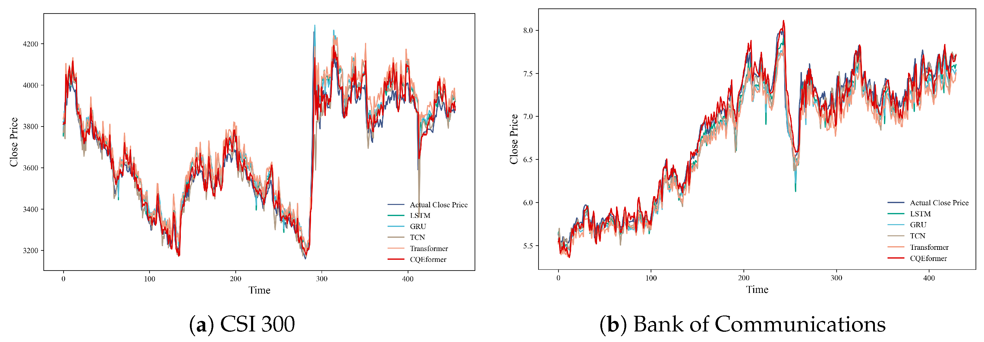
In this experiment, for two financial datasets, the time window size is fixed at 60 (approximately one quarter). We choose representative baseline models in the field of time-series prediction, including LSTM, GRU, TCN, and Transformer. These models are evaluated alongside our proposed CQEformer on all datasets, aim to validate the prediction accuracy of CQEformer and further highlight its advantages over existing approaches. The empirical results are shown in Figure 3 and Table 2.
In the multi-model comparison experiment, CQEformer achieves the best overall performance in trend fitting accuracy, local fluctuation capture, and adaptation to extreme market conditions. This superiority is visually illustrated in Figure 3 and quantitatively supported in Table 2. Across the two datasets, CQEformer reduces the MSE by an average of 38.90% compared to all baseline models. Benefiting from the causal residual embedding mechanism, the model quickly responds to sudden changes, effectively captures long-term fluctuation patterns, and demonstrates substantially higher robustness compared with the baseline models.
In contrast, the Transformer, although effective in trend fitting, exhibits a lagged response and low accuracy in capturing instantaneous fluctuations. LSTM and GRU, while computationally efficient and stable in trend tracking, lack the ability to capture fine-grained details. TCN, which excels in local feature extraction, is overly sensitive to sudden changes, leading to overreactions and reduced long-term prediction robustness.
Overall, CQEformer achieves a good balance between training time and predictive accuracy. It demonstrates clear advantages in high-precision forecasting scenarios and offers substantial potential for practical applications.
In addition to financial datasets, we also evaluated CQEformer on the public Traffic dataset to examine its cross-domain adaptability. Although traffic flow data differ from financial series in semantics, they similarly exhibit structural shifts and volatility clustering caused by external disturbances. In this experiment, the time-window length was set to 48, corresponding to approximately two days of data, to capture short-term fluctuation patterns. CQEformer achieved the best overall performance ( R 2 = 0.9299 , MSE = 4.35 × 10 5 ), reducing the average MSE of baseline models by approximately 27.29%, confirming its robustness and transferability to non-financial time series.

4.4. Time Window Sensitivity Experiment

Time window length is a key hyperparameter in time-series prediction tasks, directly affecting the model’s ability to capture historical information. To evaluate its impact for forecasting and to further verify the robustness of the proposed model, we conduct a time window sensitivity analysis by varying the window size from 10 to 100 with a step of 10, and compare the prediction performance of traditional encoder-only temporal Transformer and CQEformer.
Figure 4 summarizes the time-window sensitivity experiment. As the window size changes, CQEformer exhibits consistently low prediction error and strong stability, reducing MSE variance by 94.04% compared to the traditional Transformer, demonstrating robust adaptability to variations in time window size.

4.5. Ablation Experiment

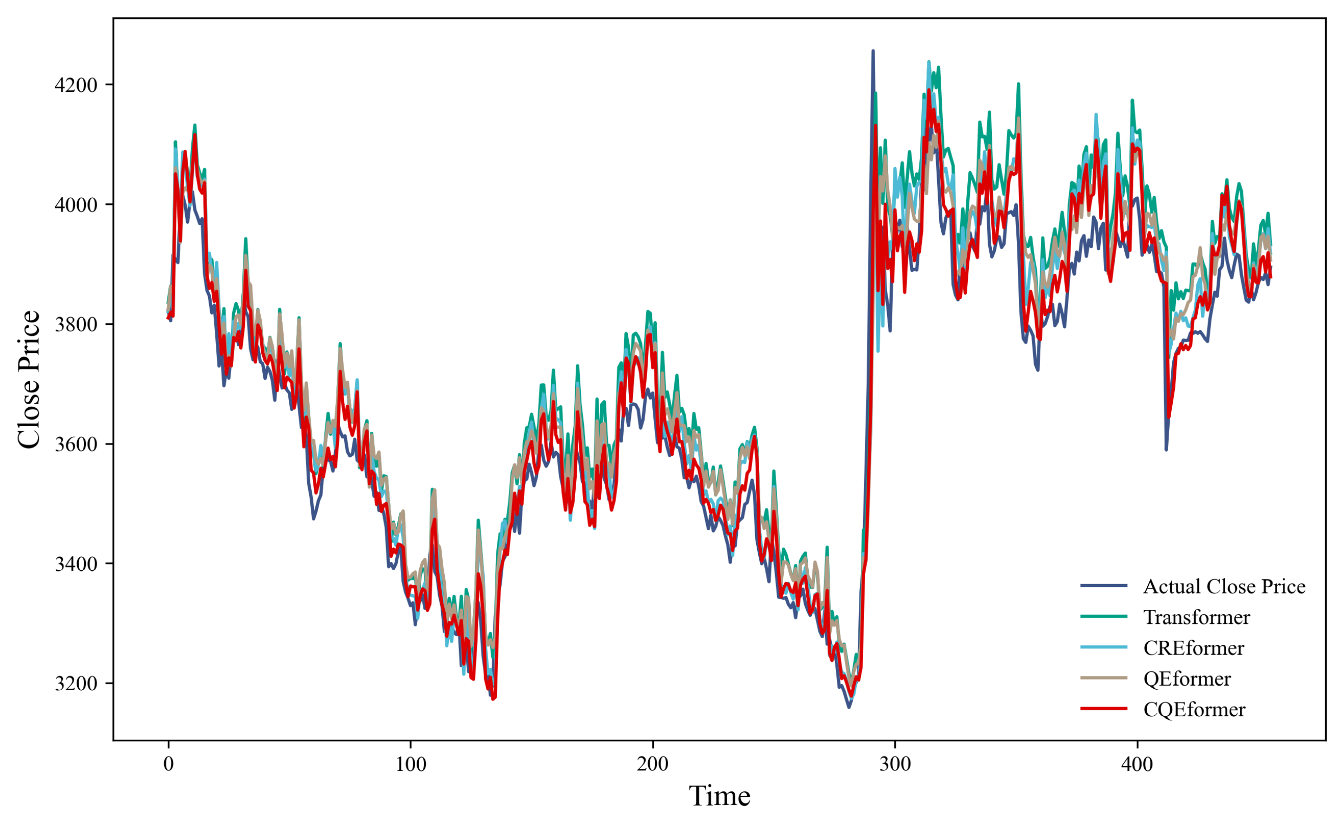
For the ablation study, we use the CSI 300 dataset with a time window of 60 and compare four variants: Encoder-Only Transformer (baseline), CREformer (causal residual embedding), QEformer (QEAttention), and CQEformer. The aim is to assess each module’s contribution, their combined effects, and validate the model design. Figure 5 and Table 3 summarize each module’s effect on the CSI 300 dataset (window size 60).
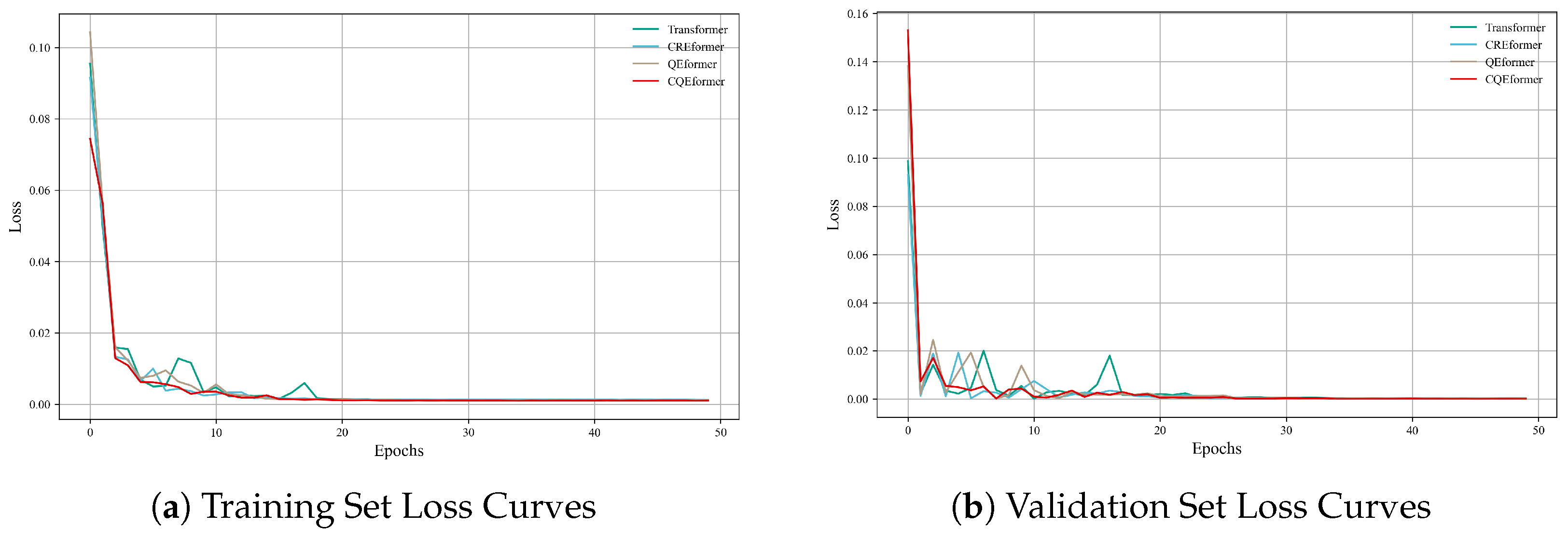
CREformer reduces MSE by 38.82% vs. Transformer, increases R 2 by 7.84%, and decreases MAPE by 28.85%, confirming its role in capturing temporal dependencies. QEformer also outperforms the baseline with MSE reduced by 32.96%, R 2 increased by 6.66%, and MAPE decreased by 21.30%, demonstrating the module’s independent value. CQEformer achieves the best results: MSE down by 60.51%, R 2 up by 12.22%, and MAPE down by 46.70%; relative to CREformer and QEformer, MSE is further reduced by 35.44% and 41.09%. Although CQEformer requires the longest training time, the substantial improvement in prediction accuracy justifies the extra cost. And CQEformer converges quickly and stably, generalizes well, and outperforms all ablation variants as shown in Figure 6.
To explore the fitting ability of ablation variants under different market risk regions, we design the experiment as follows. Using historical CSI 300 closing prices, we calculate the 20-day rolling volatility as a measure of market risk:
Risk t = E ( r t i r ¯ t ) 2 ,
where r t i is the return on day t i ( i = 0 , , 19 ), and r ¯ t = 1 20 i = 0 19 r t i .
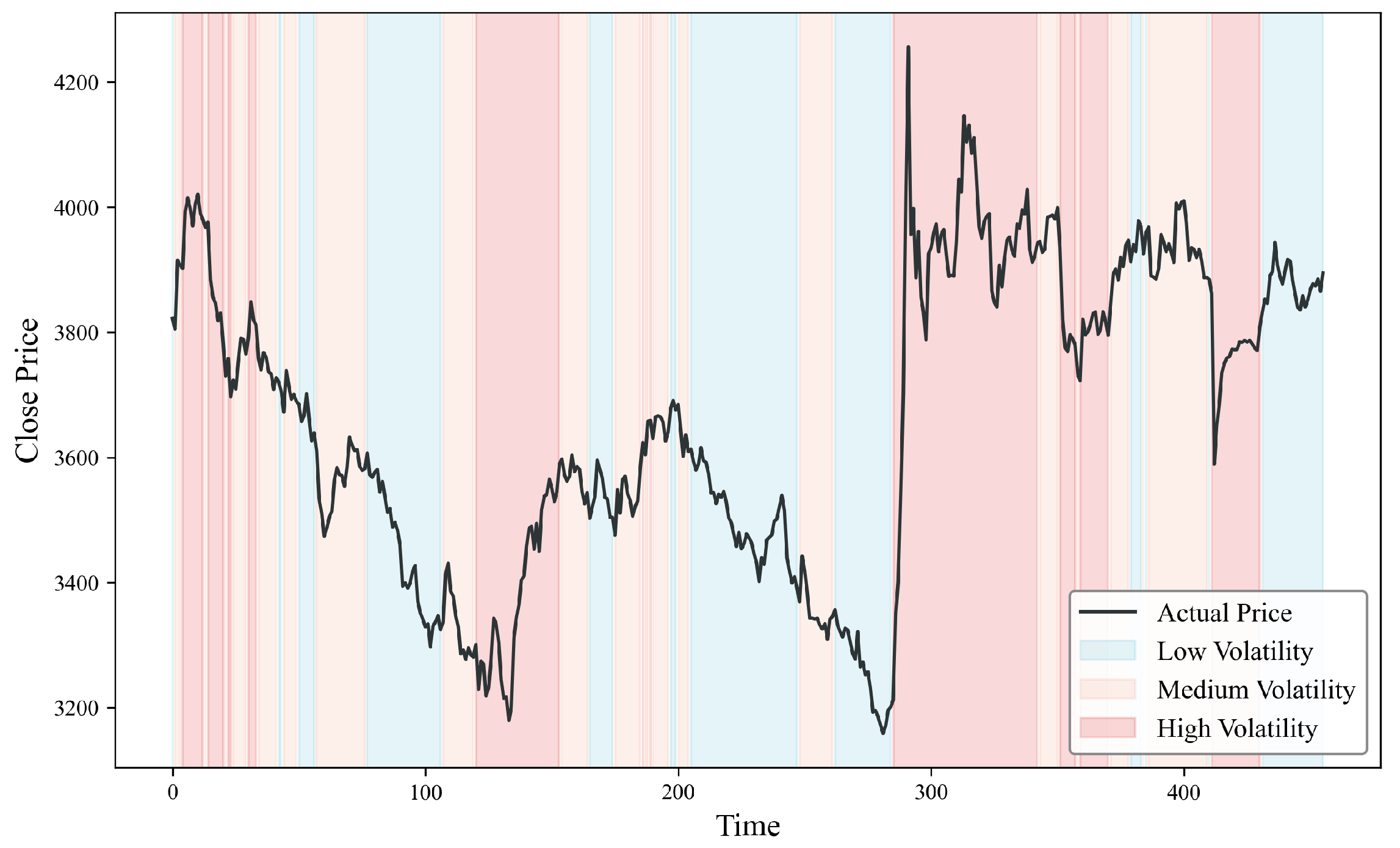
Test data are divided into three risk regions (stable, mildly volatile, highly volatile) based on the 33rd and 66th percentiles of full-series volatility: Low ( Risk 0.0077 ), Medium ( 0.0077 < Risk 0.0097 ), and High ( Risk > 0.0097 ) (Figure 7).
Using the risk region classification, we compare the MSE, MAPE, and R 2 of the ablation variants, Figure 8 and Table 4 show the prediction performance of these four models across low, medium, and high volatility regions. As volatility increases, all models exhibit higher prediction errors and lower accuracy. For CQEformer, MSE rises by 168.88% from low to high volatility, MAPE increases by 47.52%, and R 2 drops by 5.31%, indicating that higher market volatility substantially increases prediction difficulty.
Across all regions, CQEformer achieves the best performance. Compared with Transformer, its MSE decreases by 66.64%, 62.06%, and 56.70% in low, medium, and high volatility regions, respectively, demonstrating strong risk adaptability. While the improvement is slightly limited in high-volatility scenarios, CQEformer still effectively handles sudden changes, reflecting its structural robustness to high-noise and nonlinear price sequences. CREformer and QEformer perform similarly, both clearly outperforming Transformer, highlighting the effectiveness of the two enhanced modules in volatility modeling.

5. Conclusions

This study proposes CQEformer, an encoder-only model addressing the limitations of standard Transformers in nonstationary time series with structural breaks and volatility clustering, through two core innovations: causal residual embedding (CRE) and query-enhanced multi-head self-attention (QEAttention).
Key findings validate its effectiveness. In comparative experiments on the CSI 300 Index and Bank of Communications datasets, CQEformer outperforms baselines (LSTM, GRU, TCN, standard Transformer) across core metrics, achieving an average MSE reduction of 38.90%. Ablation studies confirm the modular synergy: CRE and QEAttention individually reduce MSE by 38.82% and 32.96%, respectively, while their combination yields a 60.51% reduction, highlighting the rationale of the dual-module design. CQEformer also demonstrates strong robustness to temporal window variations, outperforming the standard Transformer in adaptability. Evaluation on the public Traffic dataset further verifies its cross-domain generalization.
Theoretically, CQEformer advances nonstationary time-series prediction by integrating causal structure awareness with statistical prior guidance, effectively balancing local detail capture and global context preservation. Practically, its superior performance across financial and traffic domains underscores its potential for high-precision forecasting under dynamic, volatile conditions, while its interpretable framework aids understanding of complex temporal dynamics. Future work will focus on developing lightweight architectures, enhancing cross-domain generalization, improving long-term forecasting, and integrating multi-source information including external indicators.

Author Contributions

Conceptualization, Y.T.; Methodology, Y.T.; Software, Y.T.; Writing—Original Draft, Y.T.; Supervision, L.L.; Funding Acquisition, L.L.; Project Administration, L.L.; Writing—Review and Editing, Y.T. and L.L. All authors have read and agreed to the published version of the manuscript.

Funding

This research was funded by the National Natural Science Foundation of China (62173222) and Shanghai University of Engineering Science Horizontal Research Project (SJ20230195).

Data Availability Statement

This study used publicly available financial and traffic time series datasets obtained from open repositories, as cited in the manuscript. No new data were generated. https://github.com/akfamily/akshare (accessed on 15 June 2025). https://pems.dot.ca.gov/ (accessed on 8 November 2025).

Conflicts of Interest

The authors declare no conflicts of interest.

References

  1. Osborne, M.F.M. Periodic Structure in the Brownian Motion of Stock Prices. Oper. Res. 1962, 10, 345–379. [Google Scholar] [CrossRef]
  2. Box, G.; Jenkins, G. Time Series Analysis: Forecasting and Control; Holden-Day Series in Time Series Analysis and Digital Processing; Holden-Day: Sydney, Australia, 1970. [Google Scholar]
  3. Sims, C.A. Macroeconomics and Reality. Econometrica 1980, 48, 1–48. [Google Scholar] [CrossRef]
  4. Bollerslev, T. Generalized autoregressive conditional heteroskedasticity. J. Econom. 1986, 31, 307–327. [Google Scholar] [CrossRef]
  5. Petrica, A.C.; Stancu, S.; Tindeche, A. Limitation of ARIMA Models in Financial and Monetary Economics. Theor. Appl. Econ. 2016, XXIII, 19–42. [Google Scholar]
  6. Wang, D.; Zheng, Y.; Lian, H.; Li, G. High-Dimensional Vector Autoregressive Time Series Modeling via Tensor Decomposition. J. Am. Stat. Assoc. 2022, 117, 1338–1356. [Google Scholar] [CrossRef]
  7. Andersen, T.G.; Bollerslev, T.; Diebold, F.X.; Labys, P. Modeling and Forecasting Realized Volatility. Econometrica 2003, 71, 579–625. [Google Scholar] [CrossRef]
  8. Nguyen, T.N.; Tran, M.N.; Gunawan, D.; Kohn, R. A Statistical Recurrent Stochastic Volatility Model for Stock Markets. J. Bus. Econ. Stat. 2023, 41, 414–428. [Google Scholar] [CrossRef]
  9. Sang, S.; Li, L. A Novel Variant of LSTM Stock Prediction Method Incorporating Attention Mechanism. Mathematics 2024, 12, 945. [Google Scholar] [CrossRef]
  10. Lee, M.C. Research on the Feasibility of Applying GRU and Attention Mechanism Combined with Technical Indicators in Stock Trading Strategies. Appl. Sci. 2022, 12, 1007. [Google Scholar] [CrossRef]
  11. Vaswani, A.; Shazeer, N.; Parmar, N.; Uszkoreit, J.; Jones, L.; Gomez, A.N.; Kaiser, L.; Polosukhin, I. Attention is All you Need. In Proceedings of the Advances in Neural Information Processing Systems, Long Beach, CA, USA, 4–9 December 2017; Guyon, I., Luxburg, U.V., Bengio, S., Wallach, H., Fergus, R., Vishwanathan, S., Garnett, R., Eds.; Curran Associates, Inc.: Red Hook, NY, USA, 2017; Volume 30. [Google Scholar]
  12. Zhou, H.; Zhang, S.; Peng, J.; Zhang, S.; Li, J.; Xiong, H.; Zhang, W. Informer: Beyond Efficient Transformer for Long Sequence Time-Series Forecasting. Proc. AAAI Conf. Artif. Intell. 2021, 35, 11106–11115. [Google Scholar] [CrossRef]
  13. Zhou, T.; Ma, Z.; Wen, Q.; Wang, X.; Sun, L.; Jin, R. FEDformer: Frequency Enhanced Decomposed Transformer for Long-term Series Forecasting. In Proceedings of the 39th International Conference on Machine Learning, Baltimore, MD, USA, 17–23 July 2022; Chaudhuri, K., Jegelka, S., Song, L., Szepesvari, C., Niu, G., Sabato, S., Eds.; PMLR (Proceedings of Machine Learning Research): New York, NY, USA, 2022; Volume 162, pp. 27268–27286. [Google Scholar]
  14. Nie, Y.; Nguyen, N.H.; Sinthong, P.; Kalagnanam, J. A Time Series is Worth 64 Words: Long-term Forecasting with Transformers. In Proceedings of the Eleventh International Conference on Learning Representations, Kigali, Rwanda, 1–5 May 2023. [Google Scholar]
  15. Wu, H.; Hu, T.; Liu, Y.; Zhou, H.; Wang, J.; Long, M. TimesNet: Temporal 2D-Variation Modeling for General Time Series Analysis. In Proceedings of the Eleventh International Conference on Learning Representations, Kigali, Rwanda, 1–5 May 2023. [Google Scholar]
  16. Liu, Y.; Hu, T.; Zhang, H.; Wu, H.; Wang, S.; Ma, L.; Long, M. iTransformer: Inverted Transformers Are Effective for Time Series Forecasting. In Proceedings of the Twelfth International Conference on Learning Representations, Vienna, Austria, 7–11 May 2024. [Google Scholar]
  17. Chen, P.; Zhang, Y.; Cheng, Y.; Shu, Y.; Wang, Y.; Wen, Q.; Yang, B.; Guo, C. Pathformer: Multi-scale Transformers with Adaptive Pathways for Time Series Forecasting. In Proceedings of the Twelfth International Conference on Learning Representations, Vienna, Austria, 7–11 May 2024. [Google Scholar]
  18. Zhou, Y.; Ye, Y.; Zhang, P.; Du, X.; Chen, M. TwinsFormer: Revisiting Inherent Dependencies via Two Interactive Components for Time Series Forecasting. In Proceedings of the Thirteenth International Conference on Learning Representations, Singapore, 24–28 April 2025. [Google Scholar]
  19. Liu, Y.; Qin, G.; Huang, X.; Wang, J.; Long, M. Timer-XL: Long-Context Transformers for Unified Time Series Forecasting. In Proceedings of the Thirteenth International Conference on Learning Representations, Singapore, 24–28 April 2025. [Google Scholar]
  20. Ding, Q.; Wu, S.; Sun, H.; Guo, J.; Guo, J. Hierarchical Multi-Scale Gaussian Transformer for Stock Movement Prediction. In Proceedings of the Twenty-Ninth International Joint Conference on Artificial Intelligence, IJCAI-20, Yokohama, Japan, 11–17 July 2020; Special Track on AI in FinTech. Bessiere, C., Ed.; International Joint Conferences on Artificial Intelligence Organization: New York, NY, USA, 2020; pp. 4640–4646. [Google Scholar] [CrossRef]
  21. Zhang, Q.; Qin, C.; Zhang, Y.; Bao, F.; Zhang, C.; Liu, P. Transformer-based attention network for stock movement prediction. Expert Syst. Appl. 2022, 202, 117239. [Google Scholar] [CrossRef]
  22. Xu, H.; Xiang, L.; Ye, H.; Yao, D.; Chu, P.; Li, B. Permutation Equivariance of Transformers and its Applications. In Proceedings of the 2024 IEEE/CVF Conference on Computer Vision and Pattern Recognition (CVPR), Seattle, WA, USA, 16–22 June 2024; pp. 5987–5996. [Google Scholar] [CrossRef]
  23. van den Oord, A.; Dieleman, S.; Zen, H.; Simonyan, K.; Vinyals, O.; Graves, A.; Kalchbrenner, N.; Senior, A.; Kavukcuoglu, K. WaveNet: A Generative Model for Raw Audio. arXiv 2016, arXiv:1609.03499. [Google Scholar] [CrossRef]
  24. He, K.; Zhang, X.; Ren, S.; Sun, J. Deep Residual Learning for Image Recognition. In Proceedings of the 2016 IEEE Conference on Computer Vision and Pattern Recognition (CVPR), Las Vegas, NV, USA, 27–30 June 2016; pp. 770–778. [Google Scholar] [CrossRef]
  25. Kingma, D.P.; Ba, J. Adam: A Method for Stochastic Optimization. arXiv 2017, arXiv:1412.6980. [Google Scholar] [CrossRef]
  26. King, A. AKShare. GitHub. 2022. Available online: https://github.com/akfamily/akshare (accessed on 15 June 2025).
  27. California Department of Transportation. Traffic Dataset. In California Performance Measurement System (PeMS); California Department of Transportation: Sacramento, CA, USA, 2021. [Google Scholar]
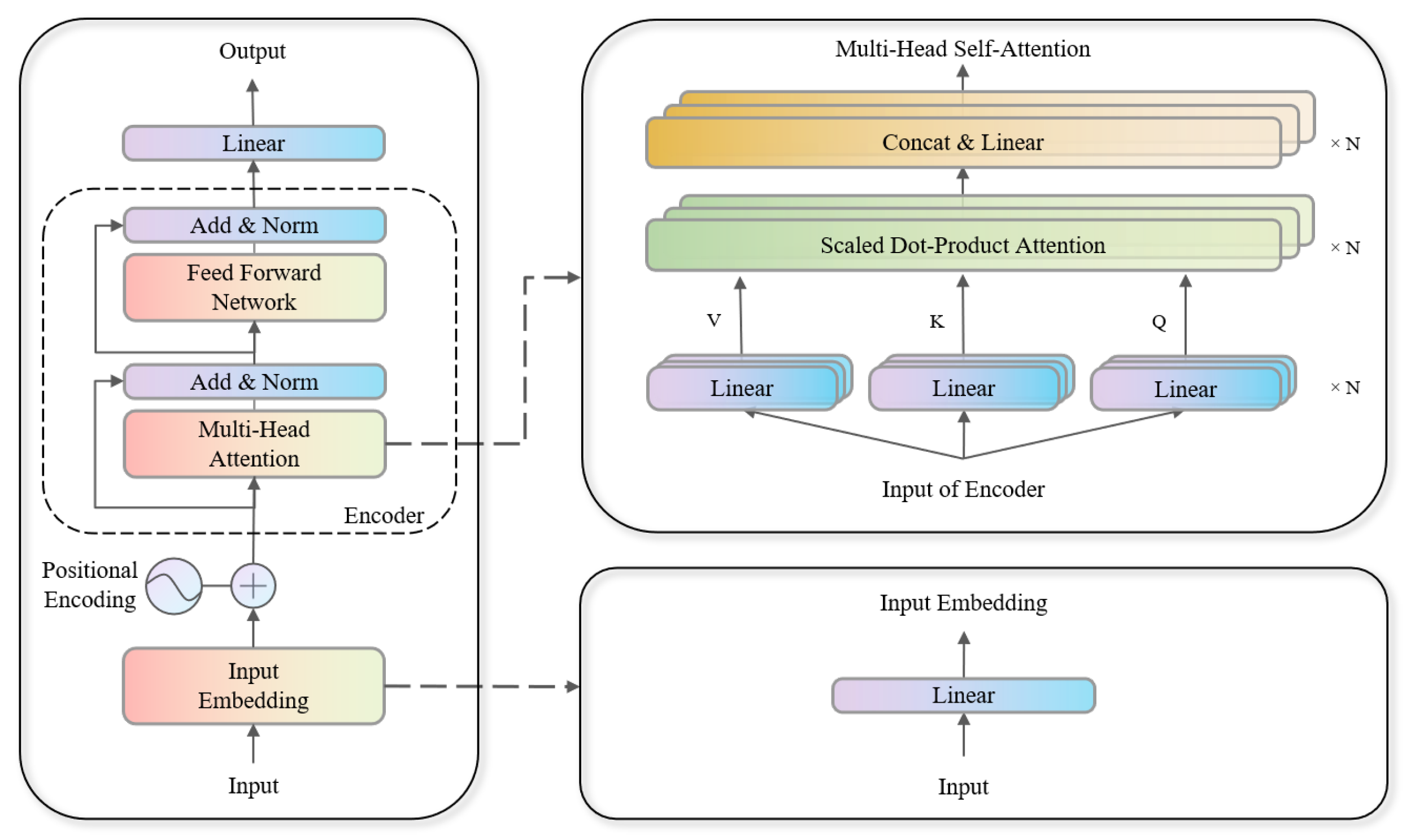
Figure 1. Network architecture of Encoder-Only Transformer.
Mathematics 13 03750 g001
Figure 2. Network architecture of CQEformer.
Mathematics 13 03750 g002
Figure 3. Multi-model prediction effect comparison on the test set.
Mathematics 13 03750 g003
Figure 4. Comparison of multi-indicator performance under different time windows.
Mathematics 13 03750 g004
Figure 5. Prediction performance comparison of ablation variants on the test set.
Mathematics 13 03750 g005
Figure 6. Loss curves of ablation variants on training and validation sets.
Mathematics 13 03750 g006
Figure 7. Volatility region distribution of the test set.
Mathematics 13 03750 g007
Figure 8. Histogram of fitting performance across volatility regions.
Mathematics 13 03750 g008
Table 1. Technical Indicator Definitions and Calculation Methods.
Indicator NameFormula
Simple Moving Average SMA t ( n ) = 1 n i = 0 n 1 P t i
Exponential Moving Average EMA t ( n ) = α · P t + ( 1 α ) · EMA t 1 ( n )
Double Exponential MA DEMA ( n ) = 2 EMA ( n ) EMA ( 2 ) ( n )
Triple Exponential MA TEMA ( n ) = 3 EMA ( n ) 3 EMA ( 2 ) ( n ) + EMA ( 3 ) ( n )
Weighted Moving Average WMA ( n ) = i = 0 n 1 ( i + 1 ) P t i i = 0 n 1 ( i + 1 )
MACD MACD t = EMA t ( 12 ) EMA t ( 26 )
MACD Signal Line Signal t = EMA t
MACD Histogram Histogram t = MACD t Signal t
Relative Strength Index RSI t ( n ) = 100 100 SumLoss t ( n ) SumGain t ( n )
Rate of Change ROC t ( n ) = P t P t n P t n × 100 %
Momentum MOM t ( n ) = P t P t n
Commodity Channel Index CCI t ( n ) = T P t SMA [ T P ] t ( n ) 0.015 MD t ( n )
Williams R WILLR t ( n ) = P t max i = 0 n 1 High t i max i = 0 n 1 High t i min i = 0 n 1 Low t i × 100
Chande Momentum Oscillator CMO t ( n ) = SumGain t ( n ) SumLoss t ( n ) SumGain t ( n ) + SumLoss t ( n ) × 100
Stochastic K K t ( n ) = P t LowestLow t ( n ) HighestHigh t ( n ) LowestLow t ( n ) × 100
Stochastic D D t ( m ) = SMA [ K t ( 14 ) ] ( m )
Symbol Explanation: P t : price at time t; n: window size; α = 2 n + 1 (smoothing factor); EMA 0 = SMA 0 ; EMA ( k ) : k-times applied EMA; SumGain t ( n ) = i = 0 n 1 max ( P t i P t i 1 , 0 ) ; SumLoss t ( n ) = i = 0 n 1 max ( P t i 1 P t i , 0 ) ; TP t = High t + Low t + P t 3 ; MD t ( n ) = 1 n i = 0 n 1 TP t i SMA [ TP ] t ( n ) .
Table 2. Multi-indicator prediction effect comparison of multi-models on the test set.
DataModelMSEMAPE R 2 Training Time
CSI 300LSTM5979.98431.74700.896738.50
GRU6791.74031.94280.882737.71
TCN5156.92411.37130.910942.26
Transformer9720.69292.29860.832068.85
CQEformer3839.06611.22520.9337106.56
Bank of CommunicationsLSTM0.02191.68190.958240.46
GRU0.02902.07080.944636.56
TCN0.01921.54260.963339.11
Transformer0.04302.57380.917964.35
CQEformer0.01631.36480.9688102.27
Table 3. Multi-indicator performance of ablation variants.
ModelMSEMAPE R 2 Training Time
Transformer9720.69292.29860.832066.63
CREformer5946.86891.63550.897273.53
QEformer6516.67241.80910.887496.61
CQEformer3839.06611.22520.9337106.12
Table 4. Fitting performance of ablation variants across volatility regions.
Volatility (Average)ModelMSEMAPE R 2
Low (0.0064)Transformer6680.71692.04890.8552
CREformer3488.82791.31860.9244
QEformer4586.18801.71050.9006
CQEformer2228.96270.99310.9517
Medium (0.0088)Transformer8523.87222.17980.8122
CREformer5165.92181.63060.8862
QEformer5061.94041.69780.8885
CQEformer3233.87621.21100.9288
High (0.0155)Transformer13840.43162.65670.7718
CREformer9097.23181.94890.8500
QEformer9805.14292.01270.8383
CQEformer5993.28611.46500.9012
Disclaimer/Publisher’s Note: The statements, opinions and data contained in all publications are solely those of the individual author(s) and contributor(s) and not of MDPI and/or the editor(s). MDPI and/or the editor(s) disclaim responsibility for any injury to people or property resulting from any ideas, methods, instructions or products referred to in the content.