Dynamics of Non-Periodic Chains with One-Sided and Two-Sided Couplings

Abstract

This paper considers the question of local dynamics of the simplest non-periodic chains of nonlinear first-order equations with two-sided couplings. The main attention is paid to the study of chains with a large number N of elements. The critical cases in the problem of stability of the zero equilibrium state are identified. Questions about bifurcations of regular and irregular solutions are considered. Analogues of normal forms are constructed, the so-called quasinormal forms, which are special nonlinear equations of parabolic type. Their nonlocal dynamics determine the local structure of solutions to the original problem. Bifurcation problems for quasinormal forms are considered, and interestingly, the boundary conditions for them are not classical. The asymptotics of both regular and irregular solutions are constructed. The latter have the most complex structure. In particular, for negative values of the coupling parameter between elements, continual families of equilibrium states, cycles, and more complex structures can arise in the chain.

1. Introduction

We consider a set of identical elements that are described by the simplest first order nonlinear ordinary differential equation

$$\dot{u}+au=f\left(u\right),$$

(1)

where $a>0$, and the function $f\left(u\right)$ is sufficiently smooth. It has an order of smallness higher than first at zero, i.e., in a neighborhood of the zero equilibrium state, and it is represented as follows:

$$f\left(u\right)=f_2{u}^2+f_3{u}^3+O\left(u^4\right).$$

We consider two different chains of coupled identical elements, each of which is described by Equation (1), and their difference consists only of the couplings between the elements.

The first type of chains is characterized by one-sided couplings, i.e., we consider a system of N equations

$${\dot{u}}_j+a{u}_j=f\left(u_j\right)+b{u}_{j+1},(b\ne 0),$$

(2)

where $j=1,\dots ,N,$ and, at the right end of the chain for $u_{N+1}\left(t\right)$, the following boundary condition is satisfied:

$$u_{N+1}=\gamma u_1(\gamma \ne 0).$$

(3)

The second type of chains of $N-1$ elements is due to two-sided couplings:

$${\dot{u}}_j+a{u}_j=f\left(u_j\right)+{\displaystyle \frac{1}{2}}b(u_{j-1}+u_{j+1}),$$

(4)

where $j=1,\dots ,N-1$, and, for the boundary elements $u_0$ and $u_{N+1}$, the following boundary conditions hold:

$$u_0=u_1,u_N=\gamma u_1(\gamma \ne 0).$$

(5)

Chains of the form (2) and (4) are important objects for research. They are given special attention. Such chains arise in modelling of many applied problems in radio-physics [1,2,3,4,5,6,7,8,9], laser physics [10,11,12,13], mathematical ecology [14,15], the theory of neural networks [16,17,18,19,20,21], optics [3,8,22,23], biophysics [24] and others.

Although most of the works are devoted to the study of relatively small chains, i.e., chains consisting of a small number of elements [25,26,27,28,29], a number of works [25,26,27,28,29,30,31] particularly emphasized the need to study chains with a large number of elements. We also note that chains with an infinite number of elements have also been considered [32].

The main assumption in this work is that the number of elements in the chains is sufficiently large, i.e., $N\gg 1.$ Therefore, the small parameter is the quantity

$$\epsilon =N^{-1}.$$

Let us consider the question of the behavior for sufficiently small $\epsilon$ and $t\to \infty$ of all solutions of the boundary value problems (2), (3) and (4), (5) with initial conditions from some sufficiently small neighborhood of the zero equilibrium state.

Let us introduce the boundary value problems linearized at zero for (2), (3) and (4), (5):

$${\dot{u}}_j+a{u}_j=b{u}_{j+1},u_{N+1}=\gamma u_1.$$

(6)

$${\dot{u}}_j+a{u}_j={\displaystyle \frac{1}{2}}b(u_{j-1}+u_{j+1}),u_0=u_1,u_N=\gamma u_1.$$

(7)

The characteristic equation for the boundary value problem (6) has the form

$${\left((\lambda +a)b^{-1}\right)}^N=\gamma ,$$

(8)

and the characteristic equation of the boundary value problem (7) is written in the form of two equations

$$\begin{array}{cc}\hfill {\left[g\left(\lambda \right)+{(g^2\left(\lambda \right)-1)}^{1/2}\right]}^N& =\hfill \\ \hfill & ={\displaystyle \frac{1}{2}}\{\gamma (1+g\left(\lambda \right)+{(g^2\left(\lambda \right)-1)}^{1/2})\pm \hfill \\ \hfill & \pm {\left[(\gamma (1+g\left(\lambda \right)+{(g^2\left(\lambda \right)-1)}^{1/2})\right]}^2-\hfill \\ & -4\left(g\left(\lambda \right)+{(g^2\left(\lambda \right)-1)}^{1/2}\right){\}}^{1/2}.\hfill \end{array}$$

(9)

For each of the boundary value problems (6) and (7), the following statement holds.

Proposition 1.

In the case when all roots of the characteristic equation have negative real parts that are separated from zero as $N\to \infty$, all solutions tend to zero as $t\to \infty .$ If the characteristic equation has a root with a positive real part separated from zero as $N\to \infty$, then the zero solution is unstable.

It is convenient to relabel the elements $u_j\left(t\right)$ using a function of two variables $u_j\left(t\right)=u(t,x_j),$ where $x_j\in [0,1]$ are uniformly distributed points on the segment $[0,1]$$x_j=2\pi j/N=2\pi i\epsilon j(j=0,1,\dots ,N).$

Passing to the continuous variable $x\in [0,1],$ the systems (2), (3) and (4), (5) can be written in the form of the equation

$${\displaystyle \frac{\partial u}{\partial t}}+au=bu(t,x+\epsilon )+f\left(u\right),$$

(10)

with boundary conditions

$$u(t,1)=\gamma u(t,0),$$

(11)

and the equation

$${\displaystyle \frac{\partial u}{\partial t}}+au={\displaystyle \frac{1}{2}}b\left(u(t,x-\epsilon )+u(t,x+\epsilon )\right)+f\left(u\right)$$

(12)

with boundary conditions

$${\displaystyle \frac{\partial u(t,x)}{\partial x}}{|}_{x=0}=0,u(t,1)=\gamma u(t,0),$$

(13)

respectively.

The boundary value problems linearized at zero for $x=x_j$ have the respective forms

$${\displaystyle \frac{\partial v}{\partial t}}+av=bv(t,x+\epsilon ),v(t,1)=\gamma v(t,0),$$

(14)

$${\displaystyle \frac{\partial v}{\partial t}}+av={\displaystyle \frac{1}{2}}b\left(v(t,x-\epsilon )+v(t,x+\epsilon )\right),{\displaystyle \frac{\partial v}{\partial x}}{|}_{x=0}=0,v(t,1)=\gamma v(t,0).$$

(15)

Obviously, for the boundary value problems (12), (13), an analogue of Proposition 1 holds.

Let us formulate a simple statement.

Theorem 1.

Let $\left|b\right|<a$. Then, all roots of the characteristic Equations (8) and (9) have negative real parts and are separated from zero as $\epsilon \to 0.$ If $\left|b\right|>a,$ then among the roots of the characteristic Equations (8) and (9), where there is a root with positive real part separated from zero as $\epsilon \to 0$.

The paper is devoted to the study of local dynamics of the boundary value problems (10), (11) and (12), (13) in critical cases when the values of the parameter $\left|b\right|$ are asymptotically close to the value of the parameter a as $\epsilon \to 0$.

It consists of two sections. The first section investigates equations with one-sided couplings, whereas the second investigates equations with two-sided couplings.

The standard methodology for studying the behavior of solutions in critical cases is the application of methods of local invariant manifolds and the method of normal forms (see, for example, [33,34]). Using the first of these methods, the original system is reduced to a simpler one whose dimension coincides with that of the critical case, and, using the method of normal forms, the latter is transformed into the most convenient form for research. In some of the problems considered in this work, this approach is not directly applicable. The point is that the critical case can have an infinite dimension (asymptotically large as $\epsilon \to 0$). In this connection, the method of quasinormal forms developed in [14,35] is applied, i.e., the method of constructing distributed (infinite-dimensional) nonlinear boundary value problems, whose nonlocal dynamics describe the local behavior of solutions to the original problem for small values of the parameter $\epsilon .$ The main result constitutes the construction of the so-called quasinormal forms, which are analogues of normal forms for the infinite-dimensional case.

It should be especially noted that we do not study exact solutions to boundary value problems, but asymptotic solutions or families of solutions that satisfy the original boundary value problem with a high degree of accuracy.

2. Chains with One-Sided Couplings

We will consider the critical case in the stability problem when the characteristic Equation (8) has no roots with positive real parts, but there exists a root with a zero real part.

Since the parameter a is positive, for sufficiently small values of the parameter b, all roots of the characteristic Equation (8) have negative real parts. With $b^{+}$, we denote the smallest positive value of the parameter b for which the characteristic Equation (8) has a root with a zero real part. If such a value does not exist, we set $b^{+}=\infty .$ Correspondingly, with $b^{-}$, we denote the largest negative value of b (if it does not exist, we set $b^{-}=-\infty$). Thus, for $b\in (b^{-},b^{+})$, all roots have negative real parts.

Let us introduce two more quantities: ${\gamma }^{+}$ and ${\gamma }^{-},$ which are “similar” to $b^{+}$ and $b^{-}$, respectively. For small values of $\gamma$, all roots of the characteristic Equation (8) have negative real parts. With ${\gamma }^{+}$, we denote the smallest positive value of the parameter $\gamma$ for which the characteristic Equation (8) has a root with a zero real part. If such a value does not exist, we set ${\gamma }^{+}=\infty .$ Correspondingly, with ${\gamma }^{-}$, we denote the largest negative value of $\gamma$ (if it does not exists, we set ${\gamma }^{-}=-\infty$). Thus, for $\gamma \in ({\gamma }^{-},{\gamma }^{+})$, all roots of the characteristic Equation (8) have negative real parts.

In Section 2.1 and Section 2.2, we study the cases when $N=2$ and $N=3.$ In particular, for these cases, the values of $b^{\pm }$ and ${\gamma }^{\pm }$ will be determined. In Section 2.3, we present results for arbitrary $N.$ In Section 2.4, which is central to this work, it is assumed that the number of equations N is sufficiently large, i.e.,

$$N\gg 1.$$

(16)

In terms of one of the important generalizations of the chain model (10), (11), we note that the obtained results also extend to chains of equations with other one-sided couplings

$${\dot{u}}_j+a{u}_j=f\left(u_j\right)+b(u_{j+1}-u_j),$$

in which, as for the chain (10), $j=1,\dots ,N;u_{N+1}=\gamma u_1.$

We note that chains for which the “periodicity” condition is satisfied

$$u_{N+1}=u_1$$

were studied in [36]. Let us immediately emphasize that the boundary condition (3) (11) for $\gamma \ne 1$ fundamentally complicates the dynamic properties of the system (2) (10).

2.1. The Case $N=2$

This case is the simplest. We consider a system of two equations

$$\begin{array}{cc}\hfill {\dot{u}}_1+a{u}_1=& f\left(u_1\right)+b{u}_2,\hfill \\ \hfill {\dot{u}}_2+a{u}_2=& f\left(u_2\right)+b\gamma u_1.\hfill \end{array}$$

(17)

For $\gamma <0$, we have $b^{\pm }=\pm \infty .$ Thus, for all b, the roots of the characteristic equation for (15) have negative real parts.

Let

$$\gamma >0.$$

Then $b^{\pm }=\pm a{\left(\sqrt{\gamma }\right)}^{-1}$ ($\sqrt{\gamma }>0$ is the arithmetic root of $\gamma$). For $b=b^{\pm }$, the linear system (6) (for $N=2$) has constant solutions

$$\left(\begin{array}{c}{u}_{10}\\ u_{20}\end{array}\right)=\left(\begin{array}{c}{b}^{\pm }\\ a\end{array}\right)·const.$$

We arbitrarily fix the value of $b_1$ and introduce a small parameter $\epsilon :0<\epsilon \ll 1.$ Let us set in (17)

$$b=b^{\pm }+\epsilon b_1.$$

(18)

Then, in the characteristic Equation (8) corresponding to (14), there is one negative root (separated from zero, as $\epsilon \to 0$) and one root ${\lambda }_0\left(\epsilon \right)$ close to zero:

$${\lambda }_0\left(\epsilon \right)=\epsilon b_1\sqrt{\gamma }+O\left({\epsilon }^2\right).$$

For small $\epsilon$, in the phase space of system (17), there exists a local invariant one-dimensional stable integral manifold (see, for example, [33]), on which system (17) (under a certain non-degeneracy condition) takes the form of a scalar ordinary differential equation up to terms of order $O\left(\epsilon \right)$

$${\displaystyle \frac{d\xi }{d\tau }}=b_1\sqrt{\gamma }\xi +a\left(1+{\left(\sqrt{\gamma }\right)}^{-1}\right){\xi }^2,$$

(19)

where $\tau =\epsilon t$ is a “slow” time, and the function $\xi \left(\tau \right)$ is related to the solutions of (17) by the asymptotic equality

$$\left(\begin{array}{c}{u}_1(t,\epsilon )\\ u_2(t,\epsilon )\end{array}\right)=\epsilon \xi \left(\tau \right)\left(\begin{array}{c}{b}^{\pm }\\ a\end{array}\right)+O\left({\epsilon }^2\right).$$

(20)

For $b_1\ne 0$, Equation (19) has a non-zero equilibrium state ${\xi }_0=-b_1\sqrt{\gamma }{\left[a+\left(1+{\left(\sqrt{\gamma }\right)}^{-1}\right)\right]}^{-1}.$ It is stable for $b_1>0$ and unstable for $b_1<0.$ Therefore, system (17) for $\gamma >0$, under condition (18), and for sufficiently small $\epsilon$, has an equilibrium state

$$\left(\begin{array}{c}{u}_{10}\\ u_{20}\end{array}\right)=\epsilon {\xi }_0\left(\begin{array}{c}{b}^{\pm }\\ a\end{array}\right)+O\left({\epsilon }^2\right),$$

which is stable (unstable) for $b_1>0(b_1<0).$ In the considered case close to critical, Equation (19) is called the normal form. The above-mentioned non-degeneracy condition is $f_2\ne 0.$ For $f_2=0$ and $f_3\ne 0$, the changes are inessential. In the normal form, the quadratic term is replaced by a cubic one, and the asymptotic expansion, i.e., an analogue of (20), goes in powers of ${\epsilon }^{1/2}.$

Thus, the study of local dynamics of system (17) is complete.

For system (17), we give the values of ${\gamma }^{+}$ and ${\gamma }^{-}:$

$${\gamma }^{+}={\left({\displaystyle \frac{a}{b}}\right)}^2,{\gamma }^{-}=-\infty .$$

2.2. The Case $N=3$

System (2), (3) for $N=3$ takes the form

$$\begin{array}{cc}\hfill {\dot{u}}_1+a{u}_1=& f\left(u_1\right)+b{u}_2,\hfill \\ \hfill {\dot{u}}_2+a{u}_2=& f\left(u_2\right)+b{u}_3,\hfill \\ \hfill {\dot{u}}_3+a{u}_3=& f\left(u_3\right)+b\gamma u_1.\hfill \end{array}$$

(21)

For the linearized system

$$\dot{v}=A_{\gamma }v,\mathrm{where}v=(v_1,v_2,v_3),A_{\gamma }=\left(\begin{array}{ccc}-a& b& 0\\ 0& -a& b\\ b\gamma & 0& -a\end{array}\right)$$

(22)

the roots ${\lambda }_1,{\lambda }_2$, and ${\lambda }_3$ of the characteristic equation are determined by the relations

$${\lambda }_1+a=b\sqrt[3]{\gamma },{\lambda }_2+a=b\sqrt[3]{\gamma }\left(-{\displaystyle \frac{1}{2}}+i{\displaystyle \frac{\sqrt{3}}{2}}\right),{\lambda }_3+a=b\sqrt[3]{\gamma }\left(-{\displaystyle \frac{1}{2}}-i{\displaystyle \frac{\sqrt{3}}{2}}\right),$$

(23)

where $\sqrt[3]{\gamma }$ is the arithmetic root ($\sqrt[3]{\gamma }>0$ for $\gamma >0$ and $\sqrt[3]{\gamma }<0$ for $\gamma <0$).

For the values of ${\gamma }^{\pm }$, we have

$${\gamma }^{+}=\left\{\begin{array}{cc}{\displaystyle {\left(\frac{a}{b}\right)}^3,}\hfill & \mathrm{if}b>0,\hfill \\ {\displaystyle {\left(\frac{2a}{\left|b\right|}\right)}^3,}\hfill & \mathrm{if}b<0,\hfill \end{array}\right.{\gamma }^{-}=\left\{\begin{array}{cc}{\displaystyle -{\left(\frac{2a}{b}\right)}^3,}\hfill & \mathrm{if}b>0,\hfill \\ {\displaystyle {\left(\frac{a}{b}\right)}^3,}\hfill & \mathrm{if}b<0.\hfill \end{array}\right.$$

We give the values of the quantity $b^{\pm }:$

$$b^{+}=\left\{\begin{array}{cc}{\displaystyle \frac{a}{\sqrt[3]{\gamma }},}\hfill & \mathrm{if}\gamma >0,\hfill \\ {\displaystyle -\frac{2a}{\sqrt[3]{\gamma }},}\hfill & \mathrm{if}\gamma <0,\hfill \end{array}\right.b^{-}=\left\{\begin{array}{cc}{\displaystyle -\frac{2a}{\sqrt[3]{\gamma }},}\hfill & \mathrm{if}\gamma >0,\hfill \\ {\displaystyle \frac{a}{\sqrt[3]{\gamma }},}\hfill & \mathrm{if}\gamma <0.\hfill \end{array}\right.$$

Under the conditions $\gamma \in ({\gamma }^{-},{\gamma }^{+})$$\left(b\in (b^{-},b^{+})\right)$, the roots (23) have negative real parts, and, for $\gamma \in (-\infty ,{\gamma }^{-})$ and $\gamma \in ({\gamma }^{+},\infty )$$(b\in (-\infty ,b^{-})$ and $b\in (b^{+},\infty ))$, among the roots (23) there is a root with a positive real part. Under the conditions $\gamma ={\gamma }^{\pm }$$\left(b=b^{\pm }\right)$, critical cases of the zero root or critical cases of a pair of purely imaginary roots arise in the stability problem for solutions of (21). Let us consider them.

2.2.1. The Critical Case of Zero Root

This case arises under the condition when $b>0$ and $\gamma ={\gamma }^{+}$, or when $b<0$ and $\gamma ={\gamma }^{-}.$ We limit ourselves to considering only the first of the given conditions, i.e., below we assume that

$$b>0\mathrm{and}\gamma ={\gamma }^{+}={\left({\displaystyle \frac{a}{b}}\right)}^3.$$

The linear system (22) for $\gamma ={\gamma }^{+}$ has constant solutions $v=d_0=const,$ where $d_0=\left(1,a{b}^{-1},a^2{b}^{-2}\right).$

We fix arbitrarily the value of ${\gamma }_1$ and set

$$\gamma ={\gamma }^{+}+\epsilon {\gamma }_1,0<\epsilon \ll 1,$$

in (21). Then, the roots ${\lambda }_2$ and ${\lambda }_3$ have negative real parts for small $\epsilon$: $\Re {\lambda }_{2,3}=-{\displaystyle \frac{1}{2}}a+O\left(\epsilon \right),$ and for the root ${\lambda }_1\left(\epsilon \right)$, we have the asymptotic equality:

$$\lambda \left(\epsilon \right)=\epsilon {\mu }_1{\gamma }_1+O\left({\epsilon }^2\right),\mathrm{where}{\mu }_1=b^3{\left(3a^2\right)}^{-1}.$$

This implies that in a sufficiently small neighborhood of the zero equilibrium state of system (21), independent of $\epsilon$, there exists a stable local invariant one-dimensional integral manifold, on which this system can be represented up to $O\left(\epsilon \right)$ in the form of a normal form (under the fulfillment of a certain non-degeneracy condition)

$${\displaystyle \frac{d\xi }{d\tau }}=\alpha \xi +\beta {\xi }^2,\tau =\epsilon t.$$

(24)

To determine the coefficients $\alpha$ and $\beta$, we substitute into (21) the solution $u=(u_1,u_2,u_3)$ in the form of an asymptotic series

$$u(t,\epsilon )=\epsilon \xi \left(\tau \right)d_0+{\epsilon }^2{U}_2\left(\tau \right)+\dots .$$

Collecting coefficients at the first power of $\epsilon$ in the resulting formal identity, we obtain a correct equality, and taking into account the coefficients at ${\epsilon }^2,$ we arrive at a system for determining the function $U_2\left(\tau \right):$

$$A_{{\gamma }_{+}}{U}_2=-d_0{\displaystyle \frac{d\xi }{d\tau }}+f_2{\xi }^2{d}_0·d_0+b{\gamma }_1\left(\begin{array}{c}0\\ 0\\ 1\end{array}\right).$$

(25)

Here and below, multiplication of vectors is calculated coordinatewise.

System (25) is solvable if and only if its right-hand side is orthogonal to the vector $h_0=(1,b{a}^{-1},b^2{a}^{-2})$—a non-zero solution of the homogeneous adjoint equation $A^{*}{h}_0=0.$ Taking this into account, we obtain that in (24)

$$\alpha ={\mu }_1{\gamma }_1=b^3{\left(3a^2\right)}^{-1}{\gamma }_1,\beta ={\displaystyle \frac{1}{3}}{f}_2(d_0·d_0,h_0).$$

(26)

The above-mentioned non-degeneracy condition consists in satisfying the inequality $f_2\ne 0.$ Using (26) in (24), we obtain a complete picture of the behavior of solutions of (24), and hence of solutions of (21) in a small neighborhood of the zero equilibrium state.

2.2.2. The Critical Case of a Pair of Purely Imaginary Roots

This case arises under the conditions

$$b<0\mathrm{and}{\gamma }^{+}={\left({\displaystyle \frac{2a}{\left|b\right|}}\right)}^3,\mathrm{or}b>0\mathrm{and}{\gamma }^{-}=-{\left({\displaystyle \frac{2a}{b}}\right)}^3.$$

Let the first of these conditions be satisfied

$$b<0,{\gamma }^{+}={\left({\displaystyle \frac{2a}{\left|b\right|}}\right)}^3.$$

Then ${\lambda }_1=-a+b\sqrt[3]{{\gamma }^{+}}<0$ and ${\lambda }_{2,3}=\pm i\sqrt{3}a.$ The linear system (22) in this case has periodic solutions

$$v_0\left(t\right)=g_{0}exp\left(ia\sqrt{3}t\right),g_0=\left(\begin{array}{c}-{{\gamma }^{+}}^{1/3}(1+i\sqrt{3})\\ {{\gamma }^{+}}^{2/3}\\ -{\displaystyle \frac{1}{2}}+i{\displaystyle \frac{\sqrt{3}}{2}}\end{array}\right).$$

We fix arbitrarily the value of ${\gamma }_1$ and set

$$\gamma ={\gamma }^{+}+\epsilon {\gamma }_1,0<\epsilon \ll 1,$$

in (21) and (22). For all sufficiently small $\epsilon$, in a sufficiently small neighborhood of the zero equilibrium state of (21), independent of $\epsilon$, there exists (see, for example, [33]) a two-dimensional stable locally invariant integral manifold, on which system (21) can be represented up to terms of order $\epsilon$ in the form of a normal form—complex scalar ordinary differential equation of the first order of the form

$${\displaystyle \frac{d\xi }{d\tau }}=\delta \xi +\sigma \xi {\left|\xi \right|}^2,\tau =\epsilon t.$$

(27)

To determine the coefficients $\delta$ and $\sigma$, we substitute into (21) the solution in the form of a formal series

$$\begin{array}{cc}\hfill U(t,\epsilon )=& {\epsilon }^{1/2}\left(\xi \left(\tau \right)g_{0}exp\left(ia\sqrt{3}t\right)+\overline{\xi }\left(\tau \right){\overline{g}}_{0}exp(-ia\sqrt{3}t)\right)+\epsilon U_2(t,\tau )+\hfill \\ \hfill & +{\epsilon }^{3/2}{U}_3(t,\tau )+\dots ,\hfill \end{array}$$

where the dependence on t is $2\pi {\left(a\sqrt{3}\right)}^{-1}$-periodic. In the resulting formal identity, we collect coefficients at the same powers of $\epsilon .$ At the first step, collecting coefficients at ${\epsilon }^{1/2},$ we arrive at a correct equality. At the next step, we obtain a system of equations for determining the function $U_2(t,\tau )=U_{20}{\left|\xi \right|}^2+U_{21}{\xi }^{2}exp\left(2ia\sqrt{3}t\right)+{\overline{U}}_{21}\overline{\xi }exp(-2ia\sqrt{3}t):$

$$A{U}_{20}=f_2\left(\begin{array}{c}4{\left({\gamma }^{+}\right)}^{2/3}\\ {\left({\gamma }^{+}\right)}^{4/3}\\ 1\end{array}\right),(A-2ia\sqrt{3}I)U_{21}=f_2\left(\begin{array}{c}{\left({\gamma }^{+}\right)}^{2/3}(4+2i\sqrt{3})\\ {\left({\gamma }^{+}\right)}^{4/3}\\ 1-{\displaystyle \frac{1}{2}}i\sqrt{3}\end{array}\right).$$

From here we find that

$$U_{20}=f_2{A}^{-1}\left(\begin{array}{c}4{\left({\gamma }^{+}\right)}^{2/3}\\ {\left({\gamma }^{+}\right)}^{4/3}\\ 1\end{array}\right),U_{21}=f_2{(A-2ia\sqrt{3}I)}^{-1}\left(\begin{array}{c}{\left({\gamma }^{+}\right)}^{2/3}(4+2i\sqrt{3})\\ {\left({\gamma }^{+}\right)}^{4/3}\\ 1-{\displaystyle \frac{1}{2}}i\sqrt{3}\end{array}\right).$$

At the third step, we collect coefficients at ${\epsilon }^{3/2}.$ As a result, we arrive at a system of equations with respect to the vector function $U_3(t,\tau ),$ which we will seek in the form

$$U_3(t,\tau )=U_{31}\left(\tau \right)exp\left(ia\sqrt{3}t\right)+\overline{cc}+U_{33}\left(\tau \right)exp\left(3ia\sqrt{3}t\right)+\overline{cc}.$$

Here and below, $\overline{cc}$ denotes the term complex conjugate to the previous one.

The expression for $U_{33}\left(\tau \right)$ is easily found. We will not need it below, so we will not give it. For $U_{31}\left(\tau \right)$, we obtain a system of equations

$$\left(A_{{\gamma }_{+}}-ia\sqrt{3}I\right)U_{31}\left(\tau \right)=-b{\gamma }_1{\left({\gamma }^{+}\right)}^{1/3}(1+i\sqrt{3})\left(\begin{array}{c}0\\ 0\\ 1\end{array}\right)\xi -g_0{\displaystyle \frac{d\xi }{d\tau }}+\xi {\left|\xi \right|}^{2}B,$$

(28)

where $B=2f_2(g_0{U}_{20}+{\overline{g}}_0{U}_{21})+3f_3{g}_0·g_0·{\overline{g}}_0.$

A necessary and sufficient condition for the solvability of this system is that the right-hand side of (28) is orthogonal to the vector h—a non-zero solution of the homogeneous adjoint equation $A_{{\gamma }_{+}}h=-ia\sqrt{3}h.$ We find that $h=\left({(1+i\sqrt{3})}^2{a}^2,(1+i\sqrt{3})ab,b^2\right).$

As a result, for determining $\xi \left(\tau \right)$, we obtain Equation (27), in which

$$\delta =b^2{\left(6a\right)}^{-1}(1+i\sqrt{3}){\gamma }_1,\sigma =(B,h){\left((g_0,h)\right)}^{-1}.$$

As an example, we formulate one result.

Theorem 2.

Let the parameters ${\gamma }_1,f_2$, and $f_3$ be such that $\Re \delta >0$ and $\Re \sigma <0.$ Then, Equation (27) has a stable cycle ${\rho }_{0}exp\left(i{\phi }_0\tau \right),$ where ${\rho }_0={\left(\Re \delta ·{(\Re \sigma )}^{-1}\right)}^{1/2},$$\psi =\sqrt{3}{\gamma }_1\Re \delta +{\rho }_0^2\Im \sigma ,$ and system (21) for sufficiently small ε has a stable cycle

$$u_0(t,\epsilon )={\epsilon }^{1/2}\left(g_0{\rho }_{0}exp\left((ia\sqrt{3}+\epsilon i\psi +O\left({\epsilon }^2\right))t\right)+\overline{cc}\right)+O\left(\epsilon \right).$$

2.3. The Case of Arbitrary Number N

First of all, let us determine the values of ${\gamma }^{\pm }:$

$$\begin{array}{cc}\hfill {\gamma }^{+}=& \left\{\begin{array}{cc}{\left(a{b}^{-1}\right)}^N,\hfill & \mathrm{if}b>0,\hfill \\ {\left({a\left|b\right|}^{-1}\right)}^N,\hfill & \mathrm{if}b<0\mathrm{and}N\mathrm{is}\mathrm{odd},\hfill \\ {\displaystyle {\left({a\left|b\right|}^{-1}\right)}^N{\left(cos\frac{\pi }{N}\right)}^{-N},}\hfill & \mathrm{if}b<0\mathrm{and}N\mathrm{is}\mathrm{even};\hfill \end{array}\right.\hfill \\ \hfill {\gamma }^{-}=& \left\{\begin{array}{cc}{\displaystyle -{\left(a{b}^{-1}\right)}^N{\left(cos\frac{\pi }{N}\right)}^N,}\hfill & \mathrm{if}b>0\mathrm{and}N\mathrm{is}\mathrm{even},\hfill \\ -{\left(a{b}^{-1}\right)}^N,\hfill & \mathrm{if}b>0\mathrm{and}N\mathrm{is}\mathrm{odd},\hfill \\ -{\left({a\left|b\right|}^{-1}\right)}^N,\hfill & \mathrm{if}b<0\mathrm{and}N\mathrm{is}\mathrm{odd},\hfill \\ {\displaystyle -{\left({a\left|b\right|}^{-1}\right)}^N{\left(cos\frac{\pi }{N}\right)}^N,}\hfill & \mathrm{if}b<0\mathrm{and}N\mathrm{is}\mathrm{even}.\hfill \end{array}\right.\hfill \end{array}$$

Recall that for $\gamma \in ({\gamma }^{-},{\gamma }^{+})$, the zero solution of system (6) is asymptotically stable, and for $\gamma <{\gamma }^{-}$ or $\gamma >{\gamma }^{+}$, it is unstable. Critical cases in the stability problem for the zero equilibrium state arise for $\gamma ={\gamma }^{+}$ or for $\gamma ={\gamma }^{-}.$ In this section, we consider the local dynamics of system (6) in cases close to critical.

Let us give several formulas that will be needed later. Let ${\gamma }_N$ be the arithmetic root of N-th degree from $\left|\gamma \right|.$ We set

$$\begin{array}{c}\hfill {\gamma }_0=\left\{\begin{array}{cc}{\gamma }_N,\hfill & \mathrm{if}\gamma >0,\hfill \\ {\displaystyle {\gamma }_{N}exp\left(i\frac{\pi }{N}\right),}\hfill & \mathrm{if}\gamma <0\hfill \end{array}\right.\end{array}$$

and let

$${\displaystyle {\alpha }_k={\gamma }_{0}exp\left(\frac{2\pi ik}{N}\right),k=1,\dots ,N.}$$

Note that ${\alpha }_k^N=\gamma .$ System (2), (3) can be written in the form

$$\dot{u}=Au+F\left(u\right),$$

(29)

where

$$A=\left(\begin{array}{ccccc}-a& b& 0& \dots & 0\\ 0& -a& b& \dots & 0\\ ⋮& ⋮& \ddots & \ddots & ⋮\\ 0& 0& 0& \ddots & b\\ b\gamma & 0& 0& \dots & -a\end{array}\right),F\left(u\right)=f_{2}u·u+f_{3}u·u·u+\dots .$$

Here and below, multiplication of vectors is coordinatewise, $u=(u_1,\dots ,u_N).$

Matrix A has eigenvalues

$${\lambda }_k=-a+b{\alpha }_k(k=1,\dots ,N)$$

and corresponding eigenvectors

$$g_k=(1,{\alpha }_k,{\alpha }_k^2,\dots ,{\alpha }_k^{N-1}).$$

Note that for the matrix $A^{*}$ adjoint to A, the corresponding eigenvectors are $h_k=(1,{\alpha }_k^{-1},{\alpha }_k^{-2},\dots ,{\alpha }_k^{-(N-1)}).$

Here we assume that $N>2$ and matrix A has a zero eigenvalue, i.e.,

$$b>0\mathrm{and}\gamma ={\gamma }^{+}={\left(a{b}^{-1}\right)}^N,$$

(30)

or

$$b<0,\gamma ={\gamma }^{-}={\left(a\right|b|}^{-1}{)}^N\mathrm{and}N\mathrm{is}\mathrm{odd}.$$

We briefly consider only case (30). The eigenvalues ${\lambda }_2,\dots ,{\lambda }_N$ have negative real parts. The eigenvalue ${\lambda }_1=0$ corresponds to the eigenvector $g^0=(1,a/b,a^2/b^2,\dots ,a^{N-1}/b^{N-1}).$ We arbitrarily fix ${\gamma }_1$ and set in (3)

$$\gamma ={\gamma }^{+}+\epsilon {\gamma }_1,\mathrm{where}0<\epsilon \ll 1.$$

(31)

To find the coefficients $\alpha$ and $\beta$ of the normal form, i.e., the scalar equation

$${\displaystyle \frac{d\xi }{d\tau }}=\alpha \xi +\beta {\left|\xi \right|}^2,\tau =\epsilon t,$$

(32)

we will seek solutions $u(t,\epsilon )$ of system (29) in the form of a formal series

$$u(t,\epsilon )=\epsilon \xi \left(\tau \right)g_0+{\epsilon }^2{U}_2\left(\tau \right)+\dots .$$

Then, for $U_2\left(\tau \right)$, we obtain a system of equations

$$A{U}_2=-g_0{\displaystyle \frac{d\xi }{d\tau }}+b{\gamma }_1\left(\begin{array}{c}0\\ ⋮\\ 0\\ 1\end{array}\right)\xi +f_2{\xi }^2{g}^0·g^0.$$

For the solvability of this system, it is necessary and sufficient that its right-hand side be orthogonal to the vector $h^0=(1,b/a,b^2/a^2,\dots ,b^{N-1}/a^{N-1}).$ From here we come to the conclusion that in Equation (32)

$$\alpha ={\displaystyle \frac{a{\gamma }_1}{N{\gamma }^{+}}},\beta ={\displaystyle \frac{1-{\gamma }^{+}}{N(1-a{b}^{-1})}}.$$

(33)

Thus, it is shown that for sufficiently small $\epsilon$, the dynamic properties of solutions of (29) with initial conditions from a certain, sufficiently small neighborhood of the zero equilibrium state, independent of $\epsilon$, are described by Equation (32) with coefficients (33).

The Critical Case of a Pair of Purely Imaginary Roots

Here we assume that matrix A has a pair of purely imaginary eigenvalues $\pm i\omega$$(\omega >0),$ and all its other eigenvalues have negative real parts, i.e., the conditions are satisfied

$$b<0,{\gamma }^{+}={\left(a\right|b|}^{-1}{)}^N{\left(cos{\displaystyle \frac{\pi }{N}}\right)}^N\mathrm{and}N\mathrm{is}\mathrm{even},$$

(34)

or

$$b>0,{\gamma }^{-}=-{\left(a{b}^{-1}\right)}^N{\left(cos{\displaystyle \frac{\pi }{N}}\right)}^N\mathrm{and}N\mathrm{is}\mathrm{even},$$

or

$$b<0,{\gamma }^{-}=-{\left(a\right|b|}^{-1}{)}^N{\left(cos{\displaystyle \frac{\pi }{N}}\right)}^N\mathrm{and}N\mathrm{is}\mathrm{even}.$$

We consider only case (34). Then matrix A has eigenvalues ${\lambda }^{\pm }=\pm i\omega ,$ where $\omega =a·tg{\displaystyle \frac{\pi }{N}}.$ They correspond to eigenvectors $g_0$ and $\overline{g_0}$, respectively, and $g_0=(1,{\alpha }_{N/2},{\alpha }_{N/2}^2,\dots ,{\alpha }_{N/2}^{N-1}).$

Let (31) be satisfied for $\gamma$. The normal form describing the dynamic properties of system (29) under conditions (31) and (34) is the scalar complex Equation (27). To find the coefficients of this equation, we consider the formal series

$$\begin{array}{cc}\hfill U(t,\epsilon )=& {\epsilon }^{1/2}\left(\xi \left(\tau \right)g_{0}exp\left(i\omega t\right)+\overline{cc}\right)+\epsilon \left({\left|\xi \right|}^2{U}_{20}+{\xi }^2{U}_{21}exp\left(2i\omega t\right)+\overline{cc}\right)+\hfill \\ \hfill & +{\epsilon }^{3/2}\left(\left(U_{31}exp\left(i\omega t\right)+\overline{cc}\right)+\overline{cc}+{\xi }^3{U}_{32}exp\left(3i\omega t\right)+\overline{cc}\right)+\dots .\hfill \end{array}$$

(35)

We substitute (35) into (29) and collect coefficients at the same powers of $\epsilon .$ For ${\epsilon }^{1/2}$ we obtain a correct equality. At the next step, we find that

$$U_{20}=2f_2{A}^{-1}{g}_0·{\overline{g}}_0,U_{21}=f_2{(A-2i\omega I)}^{-1}{g}_0·g_0.$$

Collecting coefficients at ${\epsilon }^{1/2},$ we obtain equations for $U_{31}$ and $U_{32}.$ The expression for $U_{32}$ is determined simply. We omit it, since it will not needed below. For determining $U_{31}$, we arrive at the system

$$(A-i\omega I)U_{31}=B,$$

(36)

where

$$B=-g_0{\displaystyle \frac{d\xi }{d\tau }}+{\gamma }_{1}b\left(\begin{array}{c}0\\ ⋮\\ 0\\ 1\end{array}\right)\xi +2f_2{g}_0{U}_{20}+2f_2{\overline{g}}_0{U}_{21}+3f_3{g}_0·g_0·{\overline{g}}_0.$$

For the solvability of system (36), it is necessary and sufficient that vector B be orthogonal to vector $h_0$—a solution of the homogeneous adjoint equation $A^{*}h=-i\omega h.$ As a result, for the coefficients of Equation (27), we obtain the equalities

$$\delta =-b{\gamma }_1{\left({\gamma }^{+}\right)}^{(1/N-1)}{N}^{-1},$$

(37)

$$\sigma ={\displaystyle \frac{1}{N}}\left[2f_2\left((g_0{U}_{20},h_0)+({\overline{g}}_0{U}_{21},h_0)\right)+3f_3(g_0·g_0·{\overline{g}}_0,h_0)\right].$$

(38)

Under the non-degeneracy conditions $\Re \delta \ne 0$ and $\Re \sigma \ne 0$, Equation (27) with coefficients (37), (38) completely determines the local dynamics of (29). Using (35), we obtain an asymptotic representation of solutions of (29) through solutions of (27).

2.4. The Case of Sufficiently Large Values of N

The constructions for this case are significantly more complex than the previous ones. Here we assume that the value of N is sufficiently large, i.e., the quantity is sufficiently small

$$\epsilon =N^{-1}\ll 1.$$

We study the local dynamics of system (29) in this case.

First, let us formulate one simple statement.

Lemma 1.

Let the inequality be satisfied

$${a\left|b\right|}^{-1}<1.$$

(39)

Then for all sufficiently small ε, all eigenvalues of matrix A in (29) have negative real parts that are separated from zero as $\epsilon \to 0.$ If

$${a\left|b\right|}^{-1}>1,$$

(40)

then for sufficiently small values of ε, there exists an eigenvalue of matrix A whose real part is positive and separated from zero as $\epsilon \to 0.$

In case (39), for small $\epsilon$, solutions of (29) with initial conditions from a small neighborhood of the zero equilibrium state, independent of $\epsilon$ as $\epsilon \to 0$, tend to zero as $t\to \infty .$ In case (40), the zero solution of (29) is unstable, and the problem of dynamics of (29) becomes nonlocal. Therefore, below we assume that

$$\left|b\right|=a.$$

(41)

In particular, $b^{+}=a+O\left(\epsilon \right),b^{-}=-a+O\left(\epsilon \right).$ Under condition (41), matrix A in (29) has no roots with positive real parts separated from zero as $\epsilon \to 0$, but there is an asymptotically large number of roots whose real parts tend to zero as $\epsilon \to 0.$ Thus, in the stability problem for the zero equilibrium state of (29), a critical case of infinite dimension is realized. Below, we separately consider the case when $b=a$ and when $b=-a.$

We note the author’s works [9,14,17], in which the dynamic properties of systems in infinite-dimensional critical cases were studied in other cases.

We relabel the elements $u_j\left(t\right)$ using a function of two variables $u_j\left(t\right)=u(t,x_j),$ where $x_j\in [0,1)$ are uniformly distributed points on the segment $[0,1]$: $x_j=2\pi j/N=2\pi i\epsilon j$$(j=0,1,\dots ,N).$

Recall that the boundary value problem (2), (3) for $x=x_j$ can be written in the form of an equation

$${\displaystyle \frac{\partial u}{\partial t}}+au=bu(t,x+\epsilon )-f\left(u\right),$$

(42)

with boundary conditions

$$u(t,1)=\gamma u(t,0),$$

(43)

and for the Equation (42) linearized at zero, we obtain the expression

$${\displaystyle \frac{\partial v}{\partial t}}+av=bv(t,x+\epsilon ),$$

(44)

$$v(t,1)=\gamma v(t,0).$$

(45)

Equations (42) and (44) cannot be considered for a continuous argument $x\in [0,1],$ since the expressions $u(t,x+\epsilon )$ and $v(t,x+\epsilon )$ are undefined for $x+\epsilon >1.$ An exception is the case when $\gamma =1.$ It was considered in [36]. Then, assuming that $x\in (-\infty ,\infty ),$ the functions $u,v$ were considered as periodic in x with period $1.$ For the roots ${\lambda }_k\left(\epsilon \right)(k=0,\pm 1,\pm 2,\dots )$ of the characteristic equation for (44) with $\gamma =1$, the formula holds

$${\lambda }_k\left(\epsilon \right)=-a+bexp\left(2\pi ki\epsilon \right),$$

and for the corresponding eigenfunctions ${\phi }_k(t,x,\epsilon )$, we obtain the expression

$${\phi }_k(t,x,\epsilon )=exp\left({\lambda }_k\left(\epsilon \right)t\right)exp\left(2\pi ki\epsilon \right).$$

Note that under condition (41), infinitely many roots ${\lambda }_k\left(\epsilon \right)$ tend to zero as $\epsilon \to 0.$ It is important to emphasize that for $b=a+o\left(\epsilon \right)$, the functions ${\phi }_k(t,x,\epsilon )$ depend smoothly on $\epsilon$ and, which is the same, the regularity condition is satisfied

$${\phi }_k(t,x,\epsilon )={\phi }_k(t,x,0)+\epsilon {\displaystyle \frac{\partial {\phi }_k(t,x,0)}{\partial x}}+{\displaystyle \frac{1}{2}}{\epsilon }^2{\displaystyle \frac{{\partial }^2{\phi }_k(t,x,0)}{\partial x^2}}+o\left({\epsilon }^2\right).$$

If $b=-a+o\left(\epsilon \right),$ then for those integers k for which ${\lambda }_k\left(\epsilon \right)$ tend to zero as $\epsilon \to 0,$ we obtain that

$${\phi }_k(t,x,\epsilon )=exp\left(i\pi {\epsilon }^{-1}x\right){\psi }_k(t,x,\epsilon ),$$

where ${\psi }_k(t,x,\epsilon )$ depends regularly on $\epsilon .$

Let us return to the case of arbitrary $\gamma .$ For the roots ${\lambda }_k\left(\epsilon \right)$ of Equation (44), the formula holds

$${\lambda }_k\left(\epsilon \right)=-a+bexp\left(\epsilon [ln\gamma +2\pi ki]\right),$$

(46)

in which the number k takes values $k=0,\pm 1,\pm 2,\dots .$

We arbitrarily fix the value of $b_1$ and let either

$$b=a(1+\epsilon b_1),$$

(47)

or

$$b=-a(1+\epsilon b_1).$$

(48)

In case (47), we apply in (44) the regularity condition

$$v(t,x+\epsilon )=v(t,x)+\epsilon {\displaystyle \frac{\partial v(t,x)}{\partial x}}+O\left({\epsilon }^2\right).$$

Then up to $O\left({\epsilon }^2\right)$, we arrive at the equation

$${\displaystyle \frac{\partial v}{\partial t}}=\epsilon a{b}_{1}v+\epsilon a{\displaystyle \frac{\partial v}{\partial x}},v(t,1)=\gamma v(t,0).$$

In the irregular case, when condition (48) is satisfied, we obtain that

$$v(t,x)=exp\left(i\pi {\epsilon }^{-1}x\right)\overline{v}+\overline{cc}$$

and

$${\displaystyle \frac{\partial \overline{v}}{\partial t}}=\epsilon a{b}_1\overline{v}+\epsilon a{\displaystyle \frac{\partial \overline{v}}{\partial x}},(\overline{v}(t,1)+\overline{cc})exp\left(i\pi N\right)=\gamma \overline{v}(t,0)+\overline{cc}.$$

We introduce in (46) ${\lambda }_k\left(\epsilon \right)=\epsilon {\lambda }_{k1}\left(\epsilon \right).$ The real part of each ${\lambda }_{k1}\left(\epsilon \right)$ has the asymptotics

$$b_1+ln\left|\gamma \right|+O\left(\epsilon \right).$$

Hence follows a qualitative conclusion on the stability of the equilibrium state: for $b_1+ln\left|\gamma \right|>0$, the equilibrium is unstable, and for $b_1+ln\left|\gamma \right|<0$, it is stable.

Note that in case $b_1+ln\left|\gamma \right|<0$, for Equation (42) with initial conditions from a sufficiently small, independent of $\epsilon$, neighborhood of the equilibrium state, solutions tend to zero as $t\to \infty ,$ and in case $b_1+ln\left|\gamma \right|>0$, the question of dynamics of (42), (43) is not elementary. Therefore, we consider the critical case when the parameter $\gamma ={\gamma }_0$ is chosen so that

$$|{\gamma }_0|exp{b}_1=1.$$

We consider two separate cases when the parameter b is close to the parameter a and when it is close to the parameter $-a.$ In the first case, the transition will be with a regular expansion, and in the second case—with an irregular one.

2.4.1. The Case When Parameter b Is Close to Parameter a and Parameter $\gamma$ Is Positive

In this section, let us assume that equality (47) holds and

$$\gamma >0\mathrm{and}{f}_2\ne 0.$$

Then, for each number k, the following asymptotic equality holds

$${\lambda }_k\left(\epsilon \right)=\epsilon [b_1+a(ln\gamma +2\pi ki)]+O\left({\epsilon }^2\right),$$

(49)

and the eigenfunction $v_k(t,x)$ corresponding to eigenvalue ${\lambda }_k\left(\epsilon \right)$ is represented in the form

$$v_k(t,x)=exp(2\pi iakx+{\lambda }_k\left(\epsilon \right)t).$$

(50)

We use the regularity condition for the boundary value problem (42), (43), i.e., we assume

$$u(t,x+\epsilon )=u(t,x)+\epsilon {\displaystyle \frac{\partial u(t,x)}{\partial x}}+O\left({\epsilon }^2\right).$$

Let $t_1$ denote the “slow” time $t_1=\epsilon t$ and make the substitution $u(t,x)=\epsilon u_1(t_1,x).$ Then, dropping terms of order ${\epsilon }^2,$ we arrive at the model problem

$${\displaystyle \frac{\partial u_1}{\partial t_1}}=a{\displaystyle \frac{\partial u_1}{\partial x}}+a{b}_1{u}_1-f_2{u}_1^2,u_1(t_1,1)=\gamma u_1(t_1,0).$$

(51)

In (51), in addition to the trivial equilibrium state $u_1\equiv 0$, there are, generally, solutions

$$u_1=u_0\left(x\right)={[-f_2{b}_1^{-1}+c_{0}exp\left(b_{1}x\right)]}^{-1},c_0=f_2{b}_1^{-1}(\gamma -1)(\gamma exp\left(b_1\right)-1),$$

if the following conditions are met: $\gamma >0,\gamma \ne 1,-f_2+c_0{b}_{1}exp\left(b_{1}x\right)\ne 0$ for $x\in [0,1].$

Model problem (51) is an approximate problem for boundary value problem (42), (43). This means that if for $t_1\to \infty ,x\in [0,1]$ the function $u_1(t_1,x)$ tends to the function $u(t,x,\epsilon )=\epsilon u_1(\epsilon t,x),$ which satisfies (42), (43) up to $O\left({\epsilon }^2\right).$

The question of stability of equilibrium states of model problem (51) (and hence of (42), (43)) with respect to infinitely small perturbations is settled by the linearized problem.

The following lemma is formulated.

Lemma 2.

For condition $exp(-b_1)>\gamma (<\gamma )$, the equilibrium solutions in (51) and in (42), (43) are asymptotically stable (unstable).

We consider the critical case when $\gamma ={\gamma }_0,$ where

$${\gamma }_0=exp(-b_1),$$

(52)

and equilibria become degenerate. We introduce the constant $b_2$ and set

$$b=a(1+\epsilon b_1+{\epsilon }^2{b}_2).$$

(53)

For expanding the function $u(t,x+\epsilon )$, we retain in (42) terms of order ${\epsilon }^2.$ As a result, we obtain that

$${\displaystyle \frac{\partial u_1}{\partial t_1}}=a{\displaystyle \frac{\partial u_1}{\partial x}}+(a{b}_1+\epsilon a{b}_2)u_1+{\displaystyle \frac{1}{2}}a\epsilon {\displaystyle \frac{{\partial }^2{u}_1}{\partial x^2}}+f_2{u}_1^2+\epsilon f_3{u}_1^3,u_1(t_1,1)=\gamma u_1(t_1,0).$$

(54)

The problem linearized at zero for $\epsilon =0$ takes the form

$${\displaystyle \frac{\partial u_1}{\partial t_1}}=a{\displaystyle \frac{\partial u_1}{\partial x}}+a{b}_1{u}_1,u_1(t_1,1)=\gamma u_1(t_1,0).$$

(55)

Its characteristic equation

$$(\lambda -a{b}_1)v=a{\displaystyle \frac{dv}{dx}},v\left(1\right)=\gamma v\left(0\right)$$

(56)

under condition (52) has purely imaginary roots ${\lambda }_k=2\pi kia(k=0,\pm 1,\pm 2,\dots ).$

To eigenvalue ${\lambda }_k$, it corresponds the eigenfunction $v_k\left(x\right)=exp(-b_{1}x)exp\left({\lambda }_k{a}^{-1}x\right).$ We set $y=t_1-a^{-1}x$ and $w_k\left(y\right)=exp\left({\lambda }_{k}y\right).$ Then, $v_k(t_1,x)=exp(-b_{1}x)exp\left({\lambda }_{k}y\right)=exp(-b_{1}x)w_k\left(y\right).$

We construct an approximate particular solution

$$w(x,y)=exp(-b_{1}x)·\sum _{k\to -\infty }^{+\infty }{c}_k{w}_k\left(y\right)$$

which will be a solution of (55).

Based on the general method of quasinormal forms [9,14,17], we will seek a solution to problem (54) in the form of a formal series

$$u_1(\tau ,x,\epsilon )=\epsilon w(\tau ,y)exp(-b_{1}x)+{\epsilon }^2{U}_2(\tau ,x,y)+\dots ,$$

(57)

where $\tau =\epsilon t_1,$ and in variable y the function is 1-periodic.

We substitute (57) into (54) and collect coefficients at the same powers of $\epsilon .$ At the first step, collecting coefficients at the first power of $\epsilon ,$ we obtain a correct equality. At the next step, we collect coefficients at ${\epsilon }^2.$ As a result, we arrive at the equation

$$a{\displaystyle \frac{\partial U_2}{\partial x}}+a{b}_1{U}_2=\phi (\tau ,x,y),U_2\left(1\right)=\gamma U_2\left(0\right).$$

where

$$\begin{array}{cc}\hfill \phi (\tau ,x,y)=& \left[-{\displaystyle \frac{\partial w}{\partial \tau }}+{\displaystyle \frac{1}{2}}a{\displaystyle \frac{{\partial }^{2}w}{\partial y^2}}-a{b}_1{\displaystyle \frac{\partial w}{\partial y}}+({\displaystyle \frac{1}{2}}a{b}_1^2+a{b}_2)w\right]exp(-b_{1}x)+\hfill \\ \hfill & +f_{2}wexp(-2b_{1}x).\hfill \end{array}$$

(58)

We formulate an auxiliary lemma.

Lemma 3.

Let function $\phi \left(x\right)$ be continuous. Then for solvability of the problem

$$a{\displaystyle \frac{\partial \psi }{\partial x}}+a{b}_1\psi =\phi \left(x\right),\psi \left(1\right)={\gamma }_0\psi \left(0\right)+\alpha$$

it is necessary and sufficient that the equality hold

$$\underset{0}{\overset{1}{\int }}\phi \left(s\right)exp\left(b_{1}s\right)ds=a·\alpha {\gamma }_0.$$

(59)

Substituting into (59) expression (58), we arrive at the model problem for the unknown function $w(\tau ,y)$

$${\displaystyle \frac{\partial w}{\partial \tau }}={\displaystyle \frac{1}{2}}a{\displaystyle \frac{{\partial }^{2}w}{\partial y^2}}-a{b}_1{\displaystyle \frac{\partial w}{\partial y}}+({\displaystyle \frac{1}{2}}a{b}_1^2+a{b}_2)w+f_2(1-\gamma )b_1^{-1}{w}^2,$$

(60)

$$w(\tau ,y+1)\equiv w(\tau ,y).$$

(61)

The following approximation theorem holds.

Theorem 3.

Let the boundary value problem (60), (61) have a solution $w_0(\tau ,y)$ that tends as $\tau \to \infty ,y\in [0,1]$ to a certain limit. Then the function $u(t_1,x)={\epsilon }^2{w}_0({\epsilon }^{2}t,y)exp(-b_{1}x)$ satisfies the boundary value problem (42), (43) up to $o\left({\epsilon }^3\right).$

Note that in the case when $f_2=0$, in (60) the quadratic term is replaced by the corresponding cubic term. We also emphasize that the local dynamics of solutions to the boundary value problem (60), (61) can be studied using the method of invariant integral manifolds.

2.4.2. The Case When Parameter b Is Close to a and Parameter $\gamma$ Is Negative

Now let us assume that

$$\gamma <0.$$

(62)

We repeat the previous reasoning, i.e., formulas (49)–(50), the transition to the model problem (51) remain valid. Under condition (62), in (51) there is still only one equilibrium solution. We formulate it.

Lemma 4.

For condition $exp(-b_1)>\left|\gamma \right|(<|\gamma \left|\right)$, the equilibrium solution in (51) and in (42), (43) is asymptotically stable (unstable).

We consider the critical case when

$$\left|\gamma \right|={\gamma }_0=exp(-b_1).$$

(63)

Then we use equality (53). For expanding the function $u(t,x+\epsilon )$, we retain in (42) terms of order ${\epsilon }^2.$ This again leads us to the model problem (54). For the linearized model problem (55), we consider the characteristic Equation (56). Here, unlike the previous case, it has purely imaginary roots ${\lambda }_k=a\pi i(2k+1)(k=0,\pm 1,\pm 2,\dots ).$ As in the previous case, $y=t_1-a^{-1}x,w_k\left(y\right)=exp\left({\lambda }_{k}y\right).$ Then $v_k(t,x)=exp(-b_{1}x)w_k\left(y\right).$

We seek the approximate solution to boundary value problem (54) in case (62) in the form

$$u_1(\tau ,x,y)={\epsilon }^{1/2}w(\tau ,y)exp(-b_{1}x)+\epsilon u_2(\tau ,x,y)+{\epsilon }^{3/2}{u}_3(\tau ,x,y)+\dots ,$$

(64)

where $\tau =\epsilon t_1,$ and the function $w(\tau ,y)$ has the form

$$w(\tau ,y)=\sum _{k=-\infty }^{\infty }{c}_k\left(\tau \right)w_k\left(y\right).$$

We substitute the formal series (64) into (54) and collect coefficients at the same powers of $\epsilon .$ At the first step, collecting coefficients at ${\epsilon }^{1/2},$ we obtain a correct equality. At the next step, we collect coefficients at the first power of $\epsilon .$ As a result, we arrive at the model problem for finding $u_2(\tau ,x,y):$

$$a{\displaystyle \frac{\partial u_2}{\partial x}}+a{b}_1{u}_2=f_{2}exp(-2b_{1}x)w^2(\tau ,y),u_2(\tau ,1,y)=\gamma u_2(\tau ,0,y).$$

Hence it follows that

$$u_2=exp(-b_{1}x)\left[c(\tau ,y)+f_2{w}^2(\tau ,y)·b_1^{-1}(1-exp(-b_{1}x))\right],$$

where

$$c(\tau ,y)=a{f}_2{\left(b_1(\gamma -1)\right)}^{-1}{w}^2(\tau ,y)\left|\gamma \right|(1-\left|\gamma \right|).$$

At the third step, we obtain an equation for finding $u_3(\tau ,x,y).$ Without solving it (applying Lemma 3), we obtain the model problem for the unknown function $w(\tau ,y):$

$${\displaystyle \frac{\partial w}{\partial \tau }}={\displaystyle \frac{1}{2}}a{\displaystyle \frac{{\partial }^{2}w}{\partial y^2}}-a{b}_1{\displaystyle \frac{\partial w}{\partial y}}+({\displaystyle \frac{1}{2}}a{b}_1^2+a{b}_2)w+\delta w^3,$$

(65)

$$w(\tau ,y+1)\equiv -w(\tau ,y),$$

(66)

where

$$\delta =2a^3{f}_2^2\left(b_1^{-2}\right)\left[2\gamma {(1+\gamma )}^2+{3\left(\right|\gamma |}^3-1)\right].$$

The following theorem is formulated.

Theorem 4.

Let the boundary value problem (65), (66) have a solution $w_0(\tau ,y)$ tending as $\tau \to \infty ,y\in (-\infty ,\infty )$ to a certain limit. Then the function $u(t_1,x,\epsilon )={\epsilon }^{3/2}{w}_0({\epsilon }^2{t}_1,t_1+a^{-1}x)exp(-b_{1}x)$ satisfies the boundary value problem (42), (43) up to $o\left({\epsilon }^2\right).$

Note that the boundary value problem (65), (66) can also have structurally stable equilibrium states.

2.4.3. The Case When Parameter b Is Close to Parameter $-a$

Now, for an arbitrarily fixed constant $b_1$, we use condition (48). We study the linearized boundary value problem (44), (45). From the characteristic Equation (46) under condition (48), infinitely many roots ${\lambda }_k\left(\epsilon \right)(k=0,\pm 1,\pm 2,\dots )$ tend to zero as $\epsilon \to 0.$ Thus, here the critical case of infinite dimension is realized. To eigenvalue ${\lambda }_k\left(\epsilon \right)$ corresponds the eigenfunction ${\phi }_k(t,x,\epsilon ),$ which, generally speaking, does not depend regularly on the spatial variable $x.$ This means that the approximate solutions have an irregular structure.

In (44), (45), we substitute

$$u(t,x)=v(t,x)exp\left(i\pi {\epsilon }^{-1}x\right)+\overline{cc}.$$

(67)

Note that $u(t,1)=v(t,1)exp\left(i\pi N\right)+\overline{cc},$ and for $\epsilon =N^{-1},$ the boundary condition

$$v(t,1)+\overline{v}(t,1)=\gamma {(-1)}^N(v(t,0)+\overline{v}(t,0)).$$

(68)

Then for $v(t,x)$, we arrive at the equation

$${\displaystyle \frac{\partial v}{\partial t}}+av=-bv(t,x+\epsilon ).$$

(69)

Using equality (48), we find that function $v(t,x)$ is regular, i.e.,

$$v(t,x+\epsilon )=v(t,x)+\epsilon {\displaystyle \frac{\partial v(t,x)}{\partial t}}+{\displaystyle \frac{1}{2}}{\epsilon }^2{\displaystyle \frac{{\partial }^{2}v}{\partial x^2}}+\dots .$$

We substitute this expression into (42), (43). Then from representation (67), we arrive at the equation

$${\displaystyle \frac{\partial v_1}{\partial t_1}}+a{\displaystyle \frac{\partial v_1}{\partial x}}+a{b}_1{v}_1=exp(-b_{1}x)f_2{\left(v_{1}exp\left(i\pi {\epsilon }^{-1}x\right)+\overline{cc}\right)}^2$$

(70)

with boundary condition (68). Let $t_1=\epsilon t,v=\epsilon v_1.$ For this model problem, we formulate a lemma similar to Lemma 2.

Lemma 5.

For condition $exp(-b_1)>\left|\gamma \right|(<|\gamma \left|\right)$, the equilibrium solution in (70), (68) and in (42), (43) is asymptotically stable (unstable).

We focus on the most interesting critical case when equality (63) holds. In this case, the linearized boundary value problem (69), (68) has purely imaginary, periodic in y, solutions $v_{1k}=exp(-b_{1}x)w_k\left(y\right),$ where $y=t_1-a^{-1}x,$$w_k\left(y\right)=exp\left({\lambda }_{k}y\right),$ where ${\lambda }_k=2\pi ika,$ if $\gamma {(-1)}^N>0$ and ${\lambda }_k=\pi ia(2k+1),$ if $\gamma {(-1)}^N<0.$

We set

$$b=-a(1+\epsilon b_1+{\epsilon }^2{b}_2)\mathrm{and}\gamma ={\gamma }_0+\epsilon {\gamma }_1.$$

(71)

The dynamic picture in the vicinity under conditions (63) and (71) of the equilibrium state of Equations (42) and (43) with respect to infinitely small perturbations is determined by the linearized problem.

We seek in the notation already introduced the formal expansion

$$\begin{array}{cc}\hfill v(t_1,x)=& \epsilon \left(w(\tau ,y)exp(-b_{1}x)exp\left(i\pi {\epsilon }^{-1}x\right)+\overline{cc}\right)+\hfill \\ \hfill & +{\epsilon }^2[u_{20}(t,x,y)+\overline{cc}+exp\left(i\pi z\right)u_{21}(t,x,y)+\overline{cc}+\hfill \\ \hfill & +exp\left(2i\pi z\right)u_{22}(t,x,y)+\overline{cc}+exp\left(3i\pi z\right)u_{23}(t,x,y)+\overline{cc}]+\dots ,\hfill \end{array}$$

(72)

where $z=x{\epsilon }^{-1},u_1(t_1,x,y)=w(\tau ,y)exp(-b_{1}x),\tau =\epsilon t_1,w(\tau ,y)={\displaystyle \sum _{k=-\infty }^{\infty }}{c}_k\left(\tau \right)w_k\left(y\right),$ and in variable y all functions from (72) are periodic.

We consider two separate cases. In the first of them, we assume that

$${(-1)}^N{\gamma }_0>0,$$

(73)

and in the second case—the inequality holds

$${(-1)}^N{\gamma }_0<0.$$

(74)

Constructing the critical boundary value problem for condition (73). Let equality (73) hold. We substitute (72) into (42), (43) and collect coefficients at the same powers of $\epsilon .$ As a result, we obtain the equalities

$$\begin{array}{cc}\hfill & a{\displaystyle \frac{\partial u_1}{\partial x}}+a{b}_1{u}_1=0,\hfill \end{array}$$

(75)

$$\begin{array}{cc}\hfill & 2a{u}_{20}=f_2{\left|u_1\right|}^2,2a{u}_{22}=f_2{u}_1^2,\hfill \end{array}$$

(76)

$$\begin{array}{cc}\hfill & a{\displaystyle \frac{\partial u_{21}}{\partial x}}+a{b}_1{u}_{21}=\left[-(b_2+{\displaystyle \frac{1}{2}}a{b}_1^2)w-{\displaystyle \frac{\partial w}{\partial \tau }}+{\displaystyle \frac{a}{2}}{\displaystyle \frac{{\partial }^{2}w}{\partial y^2}}-a{b}_1{\displaystyle \frac{\partial w}{\partial y}}\right]·\hfill \\ \hfill & ·exp(-b_{1}x)+\left[f_2{u}_{20}+2f_2{u}_{22}+3f_3\right]·w{\left|w\right|}^{2}exp(-3b_{1}x),\hfill \end{array}$$

(77)

$$\begin{array}{cc}\hfill & a{\displaystyle \frac{\partial u_{23}}{\partial x}}+a{b}_1{u}_{23}=[a^{-1}{f}_2^2+f_3]u_1^3.\hfill \end{array}$$

(78)

From the boundary conditions, we obtain the equalities

$$\begin{array}{cc}\hfill & {(-1)}^N(u_1+\overline{cc}){|}_{x=1}={\gamma }_0(u_1+\overline{cc}){|}_{x=0},\hfill \end{array}$$

(79)

$$\begin{array}{cc}\hfill & \left(u_{20}+\overline{cc}+{(-1)}^N{u}_{21}+\overline{cc}+u_{22}+\overline{cc}+{(-1)}^N{u}_{23}+\overline{cc}\right){|}_{x=1}=\hfill \\ \hfill & ={\gamma }_0\left(u_{20}+\overline{cc}+u_{21}+\overline{cc}+u_{22}+\overline{cc}+u_{23}+\overline{cc}\right){|}_{x=0}+{\gamma }_1(u_1+\overline{cc}){|}_{x=0}.\hfill \end{array}$$

(80)

Equations (75) and (79) determine the form of unknown function $u_1.$ From (76) and (77), we find that

$$u_{20}={\left(2a\right)}^{-1}{f}_2{\left|u_1\right|}^2,u_{22}={\left(2a\right)}^{-1}{f}_2{u}_1^2,$$

(81)

and from (78) it follows that

$$u_{23}=-{\left(2a{b}_1\right)}^{-1}(f_2^2+a{f}_3)\left[exp(-3b_{1}x)-exp(-b_{1}x)\right]w^3.$$

(82)

The question of determining the coefficient $u_{21}(\tau ,x,y)$ reduces to Equation (77) and boundary condition (80). Applying Lemma 3 to the solvability condition, we obtain the model problem having the form of a complex equation

$${\displaystyle \frac{\partial w}{\partial \tau }}={\displaystyle \frac{a}{2}}{\displaystyle \frac{{\partial }^{2}w}{\partial y^2}}-a{b}_1{\displaystyle \frac{\partial w}{\partial y}}+c_{1}w+c_2{\left|w\right|}^2+c_2{w}^2+c_3{w}^3+c_{4}w{\left|w\right|}^2,$$

(83)

$$w(\tau ,y+1)\equiv w(\tau ,y),$$

(84)

where

$$\begin{array}{cc}\hfill & c_1=-({\displaystyle \frac{1}{2}}a{b}_1^2+a{b}_2)+a{\gamma }_0^2{\gamma }_1,\hfill \\ \hfill & c_2={\displaystyle \frac{1}{2}}{\gamma }_0^2{f}_2(1-{\gamma }_0),c_3=c_2,\hfill \\ \hfill & c_4=-{\left(2b_1\right)}^{-1}(f_2^2+a{f}_3){\gamma }_0^2({\gamma }_0^2-1),c_5=3{\left(2b_1\right)}^{-1}({\gamma }_0^2-1)·[f_3+a^{-1}{f}_2^2].\hfill \end{array}$$

The following approximation theorem, similar to the previous ones, holds.

Theorem 5.

Let equalities (71) and (73) be satisfied. Let function $w(\tau ,y)$ be a solution tending as $\tau \to \infty ,y\in [0,1]$ to a certain limit of the boundary value problem (83), (84). Then the function

$$\begin{array}{cc}\hfill u(t,x,y)=& \epsilon \left(w(\tau ,y)exp(-b_{1}x)exp\left(i\pi {\epsilon }^{-1}x\right)+\overline{cc}\right)+\hfill \\ \hfill & +{\epsilon }^2[u_{20}(t,x,y)+\overline{cc}+exp\left(i\pi z\right)u_{21}(t,x,y)+\overline{cc}+\hfill \\ \hfill & +exp\left(2i\pi z\right)u_{22}(t,x,y)+\overline{cc}+exp\left(3i\pi z\right)u_{23}(t,x,y)+\overline{cc}]+\dots ,\hfill \end{array}$$

satisfies the boundary value problem (42), (43) up to $O\left({\epsilon }^4\right).$

Constructing the critical boundary value problem for condition (74). Let inequality (74) hold. In this case, the calculations are significantly simpler. Preserving the introduced formal series (72), we note that in it the function $u_{21}(\tau ,x,y)$ is represented in the form of a sum of two terms

$$u_{21}(\tau ,x,y)=v_1(\tau ,x,y)+v_2(\tau ,x,y).$$

(85)

The first of them is 1-antiperiodic in y, same as function $w(\tau ,y),$ i.e., it expands into a Fourier series containing exponents $exp\left(i\pi \right(2k+1\left)\right)(k=0,\pm 1,\pm 2,\dots ).$ The second term, $v_2(\tau ,x,y)$, is 1-periodic in $y,$ i.e., it expands into a series containing only exponents $exp\left(2i\pi k\right)(k=0,\pm 1,\pm 2,\dots ).$ Substituting (72) with decomposition (85) into (42), (43) and collecting the same coefficients. As a result, we obtain equalities (75), (76), (78), (79). Equations (75), (79) determine function $u_1(\tau ,x,y)=w(\tau ,y)exp(-b_{1}x),$ and from (76) and (78), functions $u_{20},u_{22}$ and $u_{23}$ are determined by expressions (81), (82). The equation for $v_1$ is obtained by replacing in Equation (77) of $u_{21}$ by $v_1,$ and the equation for $v_2$ has the form

$$a{\displaystyle \frac{\partial v_2}{\partial x}}+a{b}_1{v}_2=0.$$

(86)

Based on the general boundary condition (80), we obtain two boundary conditions for functions $v_1$ and $v_2:$

$$\begin{array}{cc}\hfill & {(-1)}^N{v}_1{|}_{x=1}=-{(-1)}^N{u}_{23}{|}_{x=1}+\left[{\gamma }_0{v}_1+{\gamma }_0{u}_{23}+{\gamma }_0{\gamma }_1{u}_1\right]{|}_{x=0},\hfill \end{array}$$

(87)

$$\begin{array}{cc}\hfill & {(-1)}^N{v}_2{|}_{x=1}=-u_{20}{|}_{x=1}-u_{22}{|}_{x=1}+{\gamma }_0\left[v_2+u_{20}+u_{22}\right]{|}_{x=0}.\hfill \end{array}$$

(88)

From the boundary value problem (86), (88), we find that

$$v_2=v_2(\tau ,x,y)=\left(2a\right|{\gamma }_0{\left|\right)}^{-1}{f}_2{\gamma }_0(1-{\gamma }_0)w\left[\overline{w}-{\displaystyle \frac{1}{2}}w\right]exp(-b_{1}x).$$

For the solvability of the boundary value problem (77) (where $u_{21}$ is replaced by $v_1$), (87), as follows from Lemma 3, it is necessary and sufficient that the following condition

$${\displaystyle \frac{\partial w}{\partial \tau }}={\displaystyle \frac{a}{2}}{\displaystyle \frac{{\partial }^{2}w}{\partial y^2}}-a{b}_1{\displaystyle \frac{\partial w}{\partial y}}+c_{1}w+c_3{w}^3+c_{4}w{\left|w\right|}^2$$

holds, with a 1-antiperiodic boundary condition

$$w(\tau ,y+1)\equiv -w(\tau ,y).$$

The following approximation theorem holds.

Theorem 6.

Let equalities (71) and (74) be satisfied. Let function $w(\tau ,y)$ be a solution tending as $\tau \to \infty ,y\in [0,1]$ to a certain limit of the boundary value problem (83), (84). Then the function

$$\begin{array}{cc}\hfill u(t,x,y)=& \epsilon \left(w(\tau ,y)exp(-b_{1}x)exp\left(i\pi {\epsilon }^{-1}x\right)+\overline{cc}\right)+\hfill \\ \hfill & +{\epsilon }^2[u_{20}(t,x,y)+\overline{cc}+exp\left(i\pi z\right)u_{21}(t,x,y)+\overline{cc}+\hfill \\ \hfill & +exp\left(2i\pi z\right)u_{22}(t,x,y)+\overline{cc}+exp\left(3i\pi z\right)u_{23}(t,x,y)+\overline{cc}]+\dots ,\hfill \end{array}$$

satisfies the boundary value problem (42), (43) up to $O\left({\epsilon }^4\right).$

• Commentary on Section 2

Chains with one-sided or unidirectional couplings between identical equilibrium states N of an autonomous system were considered. The question of local dynamics in the stability problem for equilibrium states is studied. Recall that, for $N=2$, only the critical case of a simple root occurs, and for $N=3$ only the critical case of a pair of purely imaginary roots or a simple zero root can be realized. In this section, only finite-dimensional critical cases were studied. The situation changes significantly for sufficiently large $N.$ In Section 2.4, which has no analogues, the critical case, when the parameter N is sufficiently large, is studied, i.e., the parameter $\epsilon =N^{-1}$ is sufficiently small. In this case, as the number N increases, the critical case is transformed into an infinite-dimensional one.

The main defining feature that reflects the type of realizable critical case is the following. The critical case has infinite dimension, i.e., infinitely many roots of the characteristic equation of the linearized problem tend to zero as $\epsilon \to 0.$

By applying the infinite-dimensional normalization method—specifically, the method of quasinormal forms—developed in the author’s works [9,14,17], special nonlinear partial differential equations of parabolic type with boundary conditions have been constructed. These boundary value problems contain no small parameter and their non-local dynamics govern the behavior of all solutions of the original system originating from a sufficiently small neighborhood of the equilibrium state.

The asymptotics of the leading terms in the asymptotic representation of solutions has been constructed.

3. Chains with Two-Sided Couplings

Let us now consider the case when the coupling coefficients of the boundary conditions are both nonzero.

3.1. Critical Cases for Positive Parameter b

Let parameter $b_1$ be fixed. We set

$$b=a+{\epsilon }^2{b}_1.$$

(89)

In this case, infinitely many roots of the characteristic Equation (9) tend to zero as $\epsilon \to 0,$ i.e., the critical case of infinite dimension is realized. Here, the solution of (15), describing solutions of the linearized problem, possesses regularity condition, i.e., for the regularity condition we have

$$v(t,x+\epsilon )=v(t,x)+\epsilon {\displaystyle \frac{\partial v(t,x)}{\partial x}}+{\displaystyle \frac{1}{2}}{\epsilon }^2{\displaystyle \frac{{\partial }^{2}v(t,x)}{\partial x^2}}+O\left({\epsilon }^3\right).$$

(90)

We substitute (89) and (90) into (12), (13). Then, we introduce new time $t_1={\epsilon }^{2}t$ and $u={\epsilon }^2{u}_1,$ then divide by ${\epsilon }^2$ and drop terms of order $\epsilon ,$ we arrive at the model problem

$${\displaystyle \frac{\partial u_1}{\partial t_1}}={\displaystyle \frac{a}{2}}·{\displaystyle \frac{{\partial }^2{u}_1}{\partial x^2}}+b_1{u}_1+f_2{u}_1^2,$$

(91)

$${\displaystyle \frac{\partial u_1}{\partial x}}{|}_{x=0}=0,u_1(t_1,1)=\gamma u_1(t_1,0).$$

(92)

For this model problem, a number of approximation theorems hold (see, for example, [9,14,35]). They reduce the analysis of local dynamics of solutions to the boundary value problem (12), (13) to the study of dynamics of solutions to the equilibrium state. The following approximation theorem is formulated.

Theorem 7.

Let equality (89) hold and let $u_1(t_1,x)$ be a solution tending as $t_1\to \infty ,x\in [0,1]$ to a certain limit of the boundary value problem (91), (92). Then the function $u(t,x)={\epsilon }^2{u}_1(t_1,x)$ satisfies the boundary value problem (12), (13) up to $o\left({\epsilon }^4\right).$

Note that in (91), (92) one can construct equilibrium states or an invariant integral manifold.

3.1.1. Linear Analysis

To determine stability or instability—about dynamics of solutions to the equilibrium state—of solutions to the boundary value problem (91), (92), one must investigate the linearized boundary value problem

$${\displaystyle \frac{\partial v}{\partial t_1}}={\displaystyle \frac{a}{2}}·{\displaystyle \frac{{\partial }^{2}v}{\partial x^2}}+b_{1}v=0,{\displaystyle \frac{\partial v}{\partial x}}{|}_{x=0}=0,v{|}_{x=1}=\gamma v{|}_{x=0}.$$

(93)

We introduce for it the characteristic equation. For this, we consider the boundary value problem

$${\displaystyle \frac{a}{2}}·{\displaystyle \frac{d^{2}v}{d{x}^2}}+(b_1-\lambda )v=0,{\displaystyle \frac{dv}{dx}}{|}_{x=0}=0,v\left(1\right)=\gamma v\left(0\right).$$

From the first boundary condition, it follows that the solution is $v\left(x\right)=ch\left({\left(2(\lambda -b_1)a^{-1}\right)}^{1/2}x\right),$ and from the second boundary condition we arrive at the equation

$$ch\left({\left(2(\lambda -b_1)a^{-1}\right)}^{1/2}\right)=\gamma .$$

(94)

To solve the stability question for the linearized problem (91), (92) and (93), we need to investigate the roots in more detail.

Let us introduce the case when $\left|\gamma \right|\le 1.$ This case is the simplest. Let $\beta$ be determined by the condition that $\beta \in [0,\pi ]$ and $cos\beta =\gamma$ and $sin\beta =\sqrt{1-{\gamma }^2}.$

Lemma 6.

Let $\left|\gamma \right|\le 1.$ Then for condition

$$2b_1<a{\beta }^2$$

all roots of Equation (94) have negative real parts, and for condition

$$2b_1>a{\beta }^2$$

there exists a root of (94) with positive real part. For $2b_1=a{\beta }^2$, Equation (94) has zero root, and the corresponding solution of (93) is $v_0\left(x\right)=cos\beta x.$

In the following two lemmas, we introduce the notation

$$\delta =ln\left(\left|\gamma \right|+\sqrt{{\gamma }^2-1}\right).$$

Lemma 7.

Let $\gamma >1.$ Then, for condition

$$2b_1+a{\delta }^2<0$$

all roots of Equation (94) have negative real parts, and for condition

$$2b_1+a{\delta }^2>0$$

there exists in (94) a root with a positive real part. For $2b_1+a{\delta }^2=0$, in (94), the equation has a zero root, and the corresponding solution of (93) is $v_0\left(x\right)=ch\delta x.$

Lemma 8.

Let $\gamma <-1.$ Then for condition

$$2b_1+a{\delta }^2<2{\pi }^2$$

all roots of (94) have negative real parts, and for condition

$$2b_1+a{\delta }^2>2{\pi }^2$$

there exists a root of Equation (94) with a positive real part. For

$$2b_1+a{\delta }^2=2{\pi }^2$$

in (94), there exist two purely imaginary roots ${\lambda }^{\pm }=\pm i\omega ,$ where $\omega =a\delta \pi ,$ to which correspond periodic in $t_1$ solutions of the boundary value problem (93) $w_{\pm }(t_1,x)=exp(\pm ia\delta \pi t_1)ch(\delta \pm i\pi )x.$

Collecting the results of Lemmas 6–8, we introduce a function

$$b_1\left(\gamma \right)=\left\{\begin{array}{cc}{\displaystyle \frac{1}{2}a{\beta }^2,}\hfill & \mathrm{if}\left|\gamma \right|\le 1,\hfill \\ {\displaystyle -\frac{1}{2}a{\delta }^2,}\hfill & \mathrm{if}\gamma >1,\hfill \\ {\pi }^2-{\displaystyle \frac{1}{2}}a{\delta }^2,\hfill & \mathrm{if}\gamma <-1.\hfill \end{array}\right.$$

The graph of $b_1\left(\gamma \right)$ is shown in Figure 1. For $b_1>b_1\left(\gamma \right)$, the zero solution of the boundary value problem (93) is unstable, and for $b_1<b_1\left(\gamma \right)$—solution (93) is stable. For $b_1=b_1\left(\gamma \right)$ in the stability problem for (93), a critical case is realized.

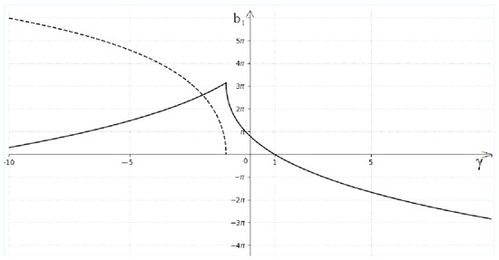
Figure 1. The graph of function $b_1\left(\gamma \right)$ is represented by continuous line, whereas the graph of function $\omega =\omega \left(\gamma \right)$ is drawn using dashed line for $\gamma \le -1$, and $\omega \left(\gamma \right)=0$ for $\gamma >-1$.

We consider these cases depending on the situation realized in the boundary value problem (91), (92) and confine ourselves to the lemmas in the stability problem.

3.1.2. Bifurcations in the Critical Case of Zero Root

We focus on the lemma in the critical case of a zero root of the characteristic equation. Let the conditions of Lemma 6 be satisfied, and let the following conditions

$$2b_{10}=a{\beta }^2,{\gamma }_0=cos\beta ,\sqrt{1-{\gamma }_0^2}=sin\beta ,\left|{\gamma }_0\right|<1,$$

(95)

hold for certain values $b_1=b_{10}$ and $\gamma ={\gamma }_0$. Let $\mu$ be a small formal positive parameter $0<\mu \ll 1.$ We set $b_1=b_{10}+\mu b_2$ and $\gamma ={\gamma }_0+\mu {\gamma }_1.$ We seek in the notation introduced the formal expansion

$$u_1(t_1,x,\mu )=\mu \xi \left(\tau \right)cos\beta x+{\mu }^2{u}_{12}(\tau ,x)+\dots ,$$

(96)

where $\tau =\mu t,$ and $\xi \left(\tau \right),u_{12}(\tau ,x),\dots$ are unknown smooth functions. We substitute (96) into (91), (92) and collect coefficients at the same powers of $\mu .$ Then, collecting coefficients at ${\mu }^2,$ we arrive at the equation

$$a\left({\displaystyle \frac{{\partial }^2{u}_{12}}{\partial x^2}}+{\beta }^2{u}_{12}\right)+\left(b_2\xi -{\displaystyle \frac{\partial \xi }{\partial \tau }}\right)cos\beta x+f_2{\xi }^2{cos}^2\beta x=0$$

(97)

with boundary conditions

$${\displaystyle \frac{\partial u_{12}}{\partial x}}{|}_{x=0}=0,u_{12}(\tau ,1)={\gamma }_0{u}_{12}(\tau ,0)+{\gamma }_1\xi .$$

(98)

From (97) and the first boundary condition in (98), we obtain an expression for $u_{12}(\tau ,x)$ with undetermined constant c

$$u_{12}(\tau ,x)={\left(a\beta \right)}^{-1}\underset{0}{\overset{x}{\int }}sin\beta (x-s)\phi \left(s\right)ds+c·cos\beta x,$$

where $\phi \left(s\right)=\left(b_2\xi -{\displaystyle \frac{\partial \xi }{\partial \tau }}\right)cos\beta s-f_2{\xi }^2{cos}^2\beta s.$ Substituting this expression into the second boundary condition (98), we obtain an equation for the unknown function $\xi \left(\tau \right):$

$${\displaystyle \frac{d\xi }{d\tau }}=g\xi -\sigma {\xi }^2,$$

(99)

where $\sigma ={\left(a\beta \right)}^{-1}{f}_2{(sin\beta )}^{-1}\underset{0}{\overset{1}{\int }}sin\beta (1-s){cos}^2\beta sds,$ $g=b_2+\beta {(sin\beta )}^{-1}{\gamma }_1.$ In the case when $g\ne 0$ and $\sigma \ne 0,$ from (99), one can determine the type of asymptotically stable, independent of parameter $\mu$, equilibrium states in (91), (92). For this, the following theorem holds.

Theorem 8.

Let equalities (95) hold and let ${\xi }_0$ be an asymptotically stable equilibrium state of (99). Then for sufficiently small values of μ, the boundary value problem (91), (92) has an asymptotically stable equilibrium state $u_0(x,\epsilon ),$ for which

$$\begin{array}{cc}\hfill & u_0(x,\epsilon )=\mu {\xi }_{0}cos\beta x+{\mu }^2{u}_{12}\left(x\right)+o\left({\mu }^3\right),\hfill \\ \hfill & u_{12}\left(x\right)={\left(a\beta \right)}^{-1}\underset{0}{\overset{x}{\int }}sin\beta (x-s)\left[b_2{\xi }_{0}cos\beta s-f_2{\xi }_0^2{cos}^2\beta s\right]ds.\hfill \end{array}$$

The proof of Theorem 8 is omitted. We note that it essentially uses properties of asymptotic stability and nonresonance of asymptotically stable equilibrium states in parabolic equations (see, for example, [33,34]) Under conditions of Lemma 7, the situation is similar. Let $b_{10}=-a{\delta }^2,b_1=b_{10}+\mu b_2,$ and in (96) replace $cos\beta x$ by $ch\delta x.$ Following the same steps, we arrive at Equation (99), where

$$g=b_2+\delta {\left(sh\delta \right)}^{-1}{\gamma }_1,\sigma ={\left(a\delta ·sh\delta \right)}^{-1}{f}_2\underset{0}{\overset{1}{\int }}sh\delta (x-s){\left(ch\delta s\right)}^{2}ds.$$

3.1.3. On Bifurcations in the Case of a Pair of Purely Imaginary Roots

Under conditions of Lemma 8, the situation is similar. Let

$$b_{10}={\pi }^2-a{\delta }^2\mathrm{and}{b}_1=b_{10}+\mu b_2,\gamma ={\gamma }_0+\mu {\gamma }_1.$$

As in the case of the Andronov—Hopf bifurcation, we consider the asymptotic expression

$$\begin{array}{cc}\hfill u_1(t_1,\tau ,x,\mu )=& {\mu }^{1/2}(\xi \left(\tau \right)exp\left(ia\delta \pi t_1\right)ch(\delta +i\pi )x+\overline{cc})+\hfill \\ \hfill & +\mu u_{12}(t_1,\tau ,x)+{\mu }^{3/2}{u}_{13}(t_1,\tau ,x)+\dots \hfill \end{array}$$

(100)

where $\tau =\mu t_1,$ and dependence on $t_1$—is periodic.

We substitute (100) into (91), (92) and collect coefficients at the same powers of $\mu .$ At the first step, we obtain a correct equality, and at the second—we arrive at the equation for finding $u_{12}:$

$${\displaystyle \frac{\partial u_{12}}{\partial t_1}}={\displaystyle \frac{a}{2}}·{\displaystyle \frac{{\partial }^2{u}_{12}}{\partial x^2}}+b_{10}{u}_{12}+f_2{\left(\xi exp\left(ia\delta \pi t_1\right)ch(\delta +i\pi )x+\overline{cc}\right)}^2.$$

$${\displaystyle \frac{\partial u_{12}}{\partial x}}{|}_{x=0}=0,u_{12}{|}_{x=1}={\gamma }_0{u}_{12}{|}_{x=0}.$$

Function $u_{12}$ is sought in the form

$$u_{12}={\left|\xi \right|}^{2}p\left(x\right)+{\xi }^{2}q\left(x\right)exp\left(2ia\delta \pi t_1\right){\left(ch(\delta +i\pi )x\right)}^2+\overline{cc}.$$

Then we continue in a similar way. We collect coefficients at ${\mu }^{3/2}$ and obtain a boundary value problem for $u_{13}.$ Without solving it (from the solvability condition—Lemma 3), we obtain a scalar complex equation for the unknown complex function $\xi \left(\tau \right)$ of the form

$${\displaystyle \frac{d\xi }{d\tau }}=g_1\xi +g_2\xi {\left|\xi \right|}^2.$$

(101)

For brevity, the expressions for coefficients, which differ little from those already given above, we omit. We also note that like in form (100) one can construct a formal solution. Note that the formulas for calculating these coefficients $g_1,g_2$ are cumbersome, but they are clear. We therefore do not give them.

Remark 1.

For $f_2\ne 0$ in Equations (99) and (101), coefficient $f_3$ does not appear. The order of parameter μ in model problems coincides with parameter ${\epsilon }^2.$ For $f_2=0$ and $f_3\ne 0$, the corresponding equations depend not on powers of ${\mu }^{1/2}$ but on powers of $\epsilon .$

Remark 2.

In the case when the nonlinearity of Equation (12) is arbitrary, i.e., when function $f\left(u\right)$ in (12) is arbitrary, the order of parameter $\mu =c{\epsilon }^2,$ corresponding to the selected decomposition, remains unchanged, but the Equations (99) and (101) depend on other more complex functions of $\xi .$ Thus, instead of (99), we obtain

$${\displaystyle \frac{d\xi }{d\tau }}=g\xi +\tilde{g}\left(\xi \right),\mathrm{where}\tilde{g}\left(\xi \right)=-{(a\delta ·sh\delta )}^{-1}\underset{0}{\overset{1}{\int }}sh\delta (x-s)f\left(\xi ch\delta s\right)ds,$$

and in the situation of Section 3.1 instead of equation of form (101), we obtain

$$\begin{array}{c}\hfill {(a\delta ·sh\delta )}^{-1}\underset{0}{\overset{1}{\int }}\underset{0}{\overset{{\left(a\delta \right)}^{-1}}{\int }}sh\left((\delta +i\pi )(1-s)\right)f(\xi exp\left(ia\delta \pi t_1\right)·\\ \hfill ·ch\left((\delta +i\pi )s+\overline{cc}\right)exp(-ia\delta \pi t_1)d{t}_{1}ds.\end{array}$$

3.2. Critical Cases for Negative Parameter b

Let us now assume

$$b=-(a+{\epsilon }^2{b}_1).$$

(102)

And in this case, infinitely many roots of the characteristic Equation (9) tend to zero as $\epsilon \to 0,$ but unlike the previous case, the eigenfunctions are rapidly oscillating and do not depend regularly on the spatial variable. Therefore, we again encounter irregular expansions. Substituting into (15)

$$v(t,x)=w(t,x)exp\left(i{\epsilon }^{-1}\pi x\right)+\overline{cc}.$$

(103)

As a result, we obtain that

$${\displaystyle \frac{\partial w}{\partial t}}+aw=-{\displaystyle \frac{b}{2}}\left(w(t,x-\epsilon )+w(t,x+\epsilon )\right).$$

(104)

Function $w(t,x)$ is complex: $w(t,x)=w_1(t,x)+i{w}_2(t,x),$ where $w_{1,2}$ are real. Boundary conditions (13) via representation (103) turn into coupled boundary conditions for $w_{1,2}(t,x):$

$${\displaystyle \frac{\partial w_1}{\partial x}}{|}_{x=0}=0,w_2{|}_{x=0}=0,$$

(105)

$${(-1)}^N{w}_1{|}_{x=1}=\gamma w_1{|}_{x=0}.$$

(106)

Then we use equality (102) and the regularity property of functions $w_{1,2}(t,x).$ Then from Equation (104), we pass to an equation with spatial differentiation

$${\displaystyle \frac{\partial w_{1,2}}{\partial t}}={\epsilon }^2\left({\displaystyle \frac{a}{2}}{\displaystyle \frac{{\partial }^2{w}_{1,2}}{\partial x^2}}+b_1{w}_{1,2}\right)$$

(107)

having discarded terms of order $o\left({\epsilon }^2\right).$ Introducing new time $t_1={\epsilon }^{2}t$, Equation (107) takes the form

$${\displaystyle \frac{\partial w_{1,2}}{\partial t_1}}={\displaystyle \frac{a}{2}}{\displaystyle \frac{{\partial }^2{w}_{1,2}}{\partial x^2}}+b_1{w}_{1,2}.$$

(108)

Equations (108) and boundary conditions (105), (106) for $w_1$ are identical to the equations considered in the previous section. The following subsections consider issues similar to those examined in Section 3.1. However, when $\gamma =\pm 1$, there are subtleties that we will not dwell on here.

3.2.1. Bifurcations in Case $|{\gamma }_0|<1$

Let us first focus on the case when $\left|\gamma \right|<1.$ The formulas needed for this case are given in Lemma 6. We set

$$\gamma ={(-1)}^N({\gamma }_0+{\epsilon }^2{\gamma }_1),\left|{\gamma }_0\right|<1,b=b_{10}+{\epsilon }^2{b}_2,$$

(109)

where ${\gamma }_0=cos\beta ,\sqrt{1-{\gamma }_0^2}=sin\beta ,2b_{10}=a{\beta }^2.$

We introduce the notation. We set $z={\epsilon }^{-1}\pi x,\tau ={\epsilon }^2{t}_1.$ Let $\xi =\xi \left(\tau \right)$ and $\eta =\eta \left(\tau \right)$ be unknown smooth complex functions that we will determine later. We seek in the notation introduced the formal expansion

$$\begin{array}{cc}\hfill w(t,x,\epsilon )=& {\epsilon }^2\left(exp\left(iz\right)[\xi w_1\left(x\right)+i\eta w_2\left(x\right)]+\overline{cc}\right)+\hfill \\ \hfill & +{\epsilon }^4[u_{20}(\tau ,x)+\overline{cc}+exp\left(iz\right)u_{21}(\tau ,x)+\overline{cc}+exp\left(2iz\right)u_{22}(\tau ,x)+\overline{cc}+\hfill \\ \hfill & +exp\left(3iz\right)u_{23}(\tau ,x)+\overline{cc}]+\dots .\hfill \end{array}$$

We substitute this expansion into the boundary value problem (12), (13) (for the case $\left|\gamma \right|<1)$ and collect the corresponding coefficients at the same powers of $\epsilon .$ From boundary conditions (13), we first obtain equalities (105), (106) with boundary conditions

$$\begin{array}{cc}\hfill & \left[(i\pi u_{21}+2i\pi u_{22}+3i\pi u_{23})+\overline{cc}\right]{|}_{x=0}=0,\hfill \end{array}$$

(110)

$$\begin{array}{cc}\hfill & \left[{\displaystyle \frac{\partial u_{20}}{\partial x}}+\overline{cc}\right]{|}_{x=0}=0,\hfill \end{array}$$

(111)

$$\begin{array}{cc}\hfill & \left[(u_{20}+{(-1)}^N{u}_{21}+u_{22}+{(-1)}^N{u}_{23})+\overline{cc}\right]{|}_{x=1}=\hfill \\ & ={(-1)}^N{\gamma }_0\left[u_{20}+u_{21}+u_{22}+u_{23})+\overline{cc}\right]{|}_{x=0}+2{(-1)}^N{\gamma }_1\xi w_1{|}_{x=0}.\hfill \end{array}$$

(112)

From Equation (12), we arrive at the equalities

$$b_{10}{u}_{20}=f_2{|\xi w_1+i\eta w_2|}^2,b_{10}{u}_{22}=f_2{(\xi w_1+i\eta w_2)}^2,$$

$${\displaystyle \frac{a}{2}}{\displaystyle \frac{{\partial }^2{u}_{21}}{\partial x^2}}+b_{10}{u}_{21}=F_{21},$$

(113)

where

$$\begin{array}{cc}\hfill & F_{21}=-{\displaystyle \frac{\partial \xi }{\partial \tau }}{w}_1-i{\displaystyle \frac{\partial \eta }{\partial \tau }}{w}_2+{\displaystyle \frac{a}{2·4!}}\left(\xi {\displaystyle \frac{{\partial }^4{w}_1}{\partial x^4}}+i\eta {\displaystyle \frac{{\partial }^4{w}_2}{\partial x^4}}\right)+b_2(\xi w_1+i\eta w_2)+\hfill \\ \hfill & +4f_2{u}_{20}(\xi w_1+i\eta w_2)+2f_2{u}_{22}(\xi w_1-i\eta w_2)+3f_3{(\xi w_1+i\eta w_2)}^2·(\xi w_1-i\eta w_2),\hfill \end{array}$$

$${\displaystyle \frac{a}{2}}{\displaystyle \frac{{\partial }^2{u}_{23}}{\partial x^2}}+b_{10}{u}_{23}=F_{23},$$

(114)

$F_{23}=(2b_{10}^{-1}{f}_2^2+f_3){(\xi w_1+i\eta w_2)}^3.$

From (105), (106), it follows that $w_1=cos\beta x,w_2=sin\beta x.$ From (106) and (107), we find that

$$u_{20}=b_{10}^{-1}{f}_2{|\xi w_1+i\eta w_2|}^2,u_{22}=b_{10}^{-1}{f}_2{(\xi w_1+i\eta w_2)}^2.$$

(115)

Let us write the solution of Equation (114) for $u_{23}.$ By substituting it into boundary conditions for $u_{23}$, we find by simple calculation that the solution satisfies boundary conditions for $x=0,$ i.e., $u_{23}{|}_{x=0}={\displaystyle \frac{\partial u_{23}}{\partial x}}{|}_{x=0}=0.$ Then we obtain that

$$u_{23}={\displaystyle \frac{2}{a\beta }}\underset{0}{\overset{x}{\int }}sin\beta (x-s)F_{23}\left(s\right)ds.$$

(116)

Now let us study the solvability of Equation (113) for $u_{21}.$ Using equalities (109), (110)–(112) and (114)–(116), we obtain that for $u_{21}=w_{21}+i{w}_{22}$ the boundary conditions have the form

$$w_{22}{|}_{x=0}=0,{\displaystyle \frac{\partial w_{21}}{\partial x}}{|}_{x=0}=0,$$

(117)

$$\begin{array}{cc}\hfill w_{21}{|}_{x=1}=& -(u_{23}+\overline{cc}){|}_{x=1}+{\gamma }_0{w}_{21}{|}_{x=0}+{\gamma }_1{(-1)}^N\xi -\hfill \\ & -{(-1)}^N(u_{20}+\overline{cc}+u_{22}+\overline{cc}){|}_{x=1}+{\gamma }_0(u_{20}+\overline{cc}+u_{22}+\overline{cc}){|}_{x=0}.\hfill \end{array}$$

(118)

Function $u_{21}$ satisfying (113), complemented by (117), takes the form

$$u_{21}=2{\left(a\beta \right)}^{-1}\underset{0}{\overset{x}{\int }}sin\beta (x-s)F_{21}\left(s\right)ds+const·cos\beta x.$$

Then, substituting into condition (118), we obtain the equation

$$\begin{array}{cc}\hfill 2\underset{0}{\overset{1}{\int }}sin\beta (1-s)& [F_{21}\left(s\right)+\overline{cc}+F_{23}\left(s\right)+\overline{cc}]ds=\hfill \\ \hfill & =a\beta {\gamma }_1{(-1)}^N\xi +4a\beta b_{10}^{-1}{F}_2({\gamma }_0-{(-1)}^N{cos}^2\beta ){\xi }^2.\hfill \end{array}$$

From here, we arrive at the scalar real equation for $\xi =\xi \left(\tau \right):$

$${\displaystyle \frac{d\xi }{d\tau }}=g_1\xi +g_2{\xi }^2+g_3{\xi }^3,$$

(119)

where

$$\begin{array}{cc}\hfill & g_1={\displaystyle \frac{a}{4!}}{\beta }^4+2b_2-{(-1)}^{N}a\beta {\gamma }_1,\hfill \\ \hfill & g_2=4a\beta b_{10}^{-1}{F}_2\left({\gamma }_0-{(-1)}^N{cos}^2\beta \right),\hfill \\ \hfill & g_3=2\left(4b_{10}^{-1}{f}_2+3F_3\right)g_0,g_0=2{\left(a\beta \right)}^{-1}\underset{0}{\overset{1}{\int }}sin\beta (1-s){cos}^2\beta sds.\hfill \end{array}$$

Before formulating an approximation theorem, let us introduce a definition.

Proposition 2.

Function $\phi (x,\epsilon )$ of the form $\phi (x,\epsilon )={\epsilon }^2{\phi }_1(x,\epsilon )+{\epsilon }^4{\phi }_2(x,\epsilon )$ is called an asymptotically invariant equilibrium state of the boundary value problem (12), (13), if up to $o\left({\epsilon }^6\right)$ it satisfies Equation (12) and exactly satisfies boundary conditions (13).

Now let us formulate a theorem that follows from the preceding constructions.

Theorem 9.

Let equalities (102), (109) hold and let Equation (119) have an equilibrium state ${\xi }_0.$ Then the boundary value problem (12), (13) has the following asymptotically invariant equilibrium state

$$\begin{array}{cc}\hfill u(x,\epsilon )=& {\epsilon }^2\left(exp\left(iz\right)[{\xi }_{0}cos\beta x+i\eta sin\beta x]+\overline{cc}\right)+\hfill \\ \hfill & +{\epsilon }^4[u_{20}\left(x\right)+\overline{cc}+exp\left(iz\right)u_{21}\left(x\right)+\overline{cc}+exp\left(2iz\right)u_{22}\left(x\right)+\overline{cc}+\hfill \\ \hfill & +exp\left(3iz\right)u_{23}\left(x\right)+\overline{cc}],\hfill \end{array}$$

where

$$\begin{array}{cc}\hfill u_{20}=& b_{10}^{-1}{f}_2{|{\xi }_{0}cos\beta x+i\eta sin\beta x|}^2,\hfill \\ \hfill u_{21}=& {\displaystyle \frac{2}{a\beta }}\underset{0}{\overset{x}{\int }}sin\beta (x-s)[{\displaystyle \frac{a}{2·4!}}\left({\xi }_0{\beta }^{4}cos\beta x+i\eta {\beta }^{4}sin\beta x\right)+b_2({\xi }_{0}cos\beta x+i\eta sin\beta x)+\hfill \\ \hfill & +4f_2{u}_{20}({\xi }_{0}cos\beta x+i\eta sin\beta x)+2f_2{u}_{22}({\xi }_{0}cos\beta x-i\eta sin\beta x)+\hfill \\ \hfill & +3f_3{({\xi }_{0}cos\beta +i\eta sin\beta x)}^2·({\xi }_{0}cos\beta -i\eta sin\beta x)],\hfill \\ \hfill u_{22}=& b_{10}^{-1}{f}_2{({\xi }_{0}cos\beta x+i\eta sin\beta x)}^2,\hfill \\ \hfill u_{23}=& {\displaystyle \frac{2}{a\beta }}\underset{0}{\overset{x}{\int }}sin\beta (x-s)(2b_{10}^{-1}{f}_2^2+f_3){({\xi }_{0}cos\beta x+i\eta sin\beta x)}^3\left(s\right)ds,\hfill \end{array}$$

and η is a real arbitrary constant.

Note that Equation (119) can have either one equilibrium state ($\xi =0$), or none, or two equilibrium states. According to the statement of Theorem 9, we conclude that in each of these cases the family has an asymptotically invariant equilibrium state depending on the arbitrary parameter $\eta$ of asymptotically invariant equilibrium states.

Here is one remark. Instead of considering the constants values of $\eta$, one can consider time-dependent, for example, periodic, function $\eta \left(\tau \right).$

It is important to emphasize the essential dependence of asymptotic expansions on the number N of chain elements. This is because in boundary condition (106) the factor ${(-1)}^N$ appears. If for even (odd) N the critical case is realized, then for odd (even) N this does not happen, i.e., either under condition of closeness to zero of solutions tend to zero as $t\to \infty ,$ or the zero solution becomes unstable and the problem of dynamics becomes nonlocal. A similar strong dependence on N was observed in Section 2.

For condition $\gamma >1$, the situation is similar. It is described by the formulas of Lemma 3. Functions $w_1\left(x\right)$ and $w_2\left(x\right)$ are represented in this case as $ch\beta x$ and $sh\beta x$ respectively.

3.2.2. Bifurcations in the Case ${\gamma }_0<-1$

Let

$${(-1)}^N\gamma ={\gamma }_0+{\epsilon }^2{\gamma }_1,{\gamma }_0<-1,b_1=b_{10}+{\epsilon }^2{b}_2$$

(120)

and the conditions of the following lemma from Lemma 8 hold:

$$2b_{10}=2{\pi }^2-a{\delta }^2,\delta =ln\left(|{\gamma }_0|+\sqrt{{\gamma }_0^2-1}\right).$$

(121)

Then the linearized equation

$${\displaystyle \frac{\partial v}{\partial t_1}}={\displaystyle \frac{a}{2}}{\displaystyle \frac{{\partial }^{2}v}{\partial x^2}}+b_{10}v$$

has solutions $exp\left(i\omega t_1\right)ch\left(\mathrm{\Delta }x\right),exp\left(i\omega t_1\right)sh\left(\mathrm{\Delta }x\right)$$(\mathrm{\Delta }=\sqrt{\delta +i\pi })$ and, respectively, complex conjugate to them. Then the solution of Equation (104) under condition (102) will up to $O\left({\epsilon }^2\right)$ be represented in the form

$$\begin{array}{cc}\hfill v_1=& exp(i\omega t_1+iz)\left[{\xi }_{1}ch\left(\mathrm{\Delta }x\right)+{\eta }_{1}sh\left(\mathrm{\Delta }x\right)\right]+\overline{cc}+\hfill \\ \hfill & +exp(i\omega t_1-iz)\left[{\xi }_{2}ch\left(\mathrm{\Delta }x\right)+{\eta }_{2}sh\left(\mathrm{\Delta }x\right)\right]+\overline{cc},\hfill \end{array}$$

(122)

where ${\xi }_{1,2}$ and ${\eta }_{1,2}$ are independent complex constants. From the first boundary condition (105) and (106), we obtain the equalities

$${\xi }_1={\xi }_2,{\eta }_1=-{\eta }_2,{(-1)}^N({\xi }_1+{\xi }_2)={\gamma }_0({\xi }_1+{\xi }_2).$$

Eliminating the indices, replacing indices 1 and 2 in the notation ${\xi }_{1,2},$${\eta }_{1,2}$ by primes, we obtain that representation (122) can be written in the form

$$\begin{array}{cc}\hfill v_1=& exp(i\omega t_1+iz)\left[\xi ch\left(\mathrm{\Delta }x\right)+\eta sh\left(\mathrm{\Delta }x\right)\right]+\overline{cc}+\hfill \\ \hfill & +exp(i\omega t_1-iz)\left[\xi ch\left(\mathrm{\Delta }x\right)-\eta sh\left(\mathrm{\Delta }x\right)\right]+\overline{cc}.\hfill \end{array}$$

Here it is assumed that the unknown complex functions $\xi =\xi \left(\tau \right)$ and $\eta =\eta \left(\tau \right)$ depend on “slow” time $\tau ={\epsilon }^2{t}_1.$

We seek approximate solutions of the boundary value problem (12), (13) in the form of a formal asymptotic expansion

$$u={\epsilon }^2{V}_1+{\epsilon }^4\left[V_{21}+V_{22}+V_{23}\right]+\dots .$$

(123)

Here the value $V_{21}$ contains the “first” harmonics, just like $V_1$, i.e.

$$V_{21}=exp(i\omega t_1+iz)W_1(\tau ,x)+\overline{cc}+exp(i\omega t_1-iz)W_2(\tau ,x)+\overline{cc}.$$

(124)

The function $V_{22}$ contains a set of “zero” and “second” harmonics

$$\begin{array}{c}\hfill V_{22}=W_{20}+\overline{cc}+W_{21}exp\left(2iz\right)+\overline{cc}+W_{22}exp\left(2i\omega t_1\right)+\overline{cc}+\\ \hfill +W_{23}exp(2i\omega t_1+2iz)+\overline{cc}+W_{24}exp(2i\omega t_1-2iz)+\overline{cc},\end{array}$$

and $V_{23}$ contains a set of “third” harmonics.

In order for expansion (123) up to $o\left({\epsilon }^6\right)$ to satisfy the boundary value problem (12), (13), it is necessary that functions $\xi \left(\tau \right)$ and $\eta \left(\tau \right)$ be solutions of a certain boundary value problem. We will not dwell on the details of the derivation of Equations (123) in (12), (13) and we collect the corresponding coefficients at the same powers of $\epsilon$ and at the same exponents. At the first step, we collect coefficients at ${\epsilon }^4.$ As a result, we arrive at the equalities

$${\displaystyle \frac{\partial V_1}{\partial t_1}}={\displaystyle \frac{a}{2}}{\displaystyle \frac{{\partial }^2{V}_1}{\partial x^2}}+b_{10}{V}_1,{\displaystyle \frac{\partial V_1}{\partial x}}{|}_{x=0}=0,V_1{|}_{x=1}={\gamma }_0{V}_1{|}_{x=0},$$

$$\begin{array}{cc}\hfill & 2a{W}_{20}=A_0(\tau ,x),2a{W}_{21}=A_1(\tau ,x),\hfill \\ \hfill & 2(a-i\omega )W_{22}=A_2(\tau ,x),2(a-i\omega )W_{23}=A_3(\tau ,x),\hfill \\ \hfill & 2(a-i\omega )W_{24}=A_4(\tau ,x).\hfill \end{array}$$

The following notations are used here

$$\begin{array}{cc}\hfill A_0(\tau ,x)=& -f_2·\left({|\xi ch\left(\mathrm{\Delta }x\right)+\eta sh\left(\mathrm{\Delta }x\right)|}^2+{|\xi ch\left(\mathrm{\Delta }x\right)-\eta sh\left(\mathrm{\Delta }x\right)|}^2\right),\hfill \\ \hfill A_1(\tau ,x)=& -f_2·\left(\xi ch\left(\mathrm{\Delta }x\right)+\eta sh\left(\mathrm{\Delta }x\right)\right)·\left(\overline{\xi }\overline{ch}\left(\mathrm{\Delta }x\right)-\overline{\eta }\overline{sh}\left(\mathrm{\Delta }x\right)\right),\hfill \\ \hfill A_2(\tau ,x)=& -f_2·\left({\left(\xi ch\left(\mathrm{\Delta }x\right)\right)}^2-{\left(\eta sh\left(\mathrm{\Delta }x\right)\right)}^2\right),\hfill \\ \hfill A_3(\tau ,x)=& -f_2·{\left(\xi ch\left(\mathrm{\Delta }x\right)+\eta sh\left(\mathrm{\Delta }x\right)\right)}^2,\hfill \\ \hfill A_4(\tau ,x)=& -f_2·{\left(\xi ch\left(\mathrm{\Delta }x\right)-\eta sh\left(\mathrm{\Delta }x\right)\right)}^2.\hfill \end{array}$$

At the next step, collecting coefficients at ${\epsilon }^6,$ we obtain a boundary value problem for $V_{21}$ and $V_{23}.$ It should be noted that the corresponding equation for $V_{23}$ is uniquely solvable and its solution is determined in closed form. We will not need it below, so we will not give it.

Let us write the boundary value problem for $V_{21}.$ First, we introduce the notation:

$$\xi ch\left(\mathrm{\Delta }x\right)+\eta sh\left(\mathrm{\Delta }x\right)=r_1,\xi ch\left(\mathrm{\Delta }x\right)-\eta sh\left(\mathrm{\Delta }x\right)=r_2$$

(125)

and also $k_1=-{\left(2a\right)}^{-1}{f}_2,k_2=-{\left(2(a+i\omega )\right)}^{-1}{f}_2.$ Then we arrive at a boundary value problem for the normalizing functions $W_1(\tau ,x)$ and $W_2(\tau ,x)$ (see Formula (124)):

$${\displaystyle \frac{a}{2}}{\displaystyle \frac{{\partial }^2{W}_j}{\partial x^2}}+(b_{10}-i\omega )W_j={\mathrm{\Phi }}_j(\tau ,x),j=1,2,$$

(126)

where

$$\begin{array}{cc}\hfill {\mathrm{\Phi }}_j(\tau ,x)=& -{\displaystyle \frac{\partial }{\partial \tau }}{r}_j+\left({\displaystyle \frac{a}{2·4!}}{\mathrm{\Delta }}^4+b_2\right)r_j+r_j\left[a_{j1}|r_1{|}^2+a_{j2}{\left|r_2\right|}^2\right],\hfill \\ \hfill a_{11}=& 3f_3+2(k_1+k_2)f_2,a_{12}=2f_3+4(k_1+k_2)f_2,\hfill \\ \hfill a_{21}=& 2f_3+4(k_1+k_2)f_2,a_{22}=3f_3+2(k_1+k_2)f_2.\hfill \end{array}$$

Solutions of system (126) for the normalizing functions $W_{1,2}(\tau ,x)$ satisfying boundary conditions at the origin have the form

$$W_j=2{\left(a\mathrm{\Delta }\right)}^{-1}\underset{0}{\overset{x}{\int }}sh\left(\mathrm{\Delta }(x-s)\right){\mathrm{\Phi }}_j(\tau ,s)ds,$$

and the first boundary condition for $x=0$ is satisfied. The boundary condition for $x=1$ takes the form $W_1(\tau ,1)+W_2(\tau ,1)={\gamma }_1\xi ,$ i.e.,

$$2{\left(a\mathrm{\Delta }\right)}^{-1}\underset{0}{\overset{1}{\int }}sh\left(\mathrm{\Delta }(1-s)\right)\left({\mathrm{\Phi }}_1(\tau ,s)+{\mathrm{\Phi }}_2(\tau ,s)\right)ds={\gamma }_1\xi .$$

(127)

Using notation (125), for the equation obtained, we have

$${\displaystyle \frac{d\xi }{d\tau }}=p_1\xi +\xi (p_2{\left|\xi \right|}^2+p_3{\left|\eta \right|}^2)+p_4\eta {\left|\xi \right|}^2,$$

(128)

where

$$\begin{array}{cc}\hfill p_1=& {(2·4!)}^{-1}{\mathrm{\Delta }}^4+b_2,\hfill \\ \hfill p_2=& \left(18f_3+8(k_1+k_2)f_2\right)·\underset{0}{\overset{1}{\int }}sin\left(\mathrm{\Delta }(1-s)\right)·ch\left(\mathrm{\Delta }s\right)·|ch\left(\mathrm{\Delta }s\right){|}^{2}ds·\hfill \\ \hfill & ·{\left(\underset{0}{\overset{1}{\int }}sh\left(\mathrm{\Delta }(1-s)\right)ch\left(\mathrm{\Delta }s\right)ds\right)}^{-1},\hfill \\ \hfill p_3=& \left(12f_3+8(k_1+k_2)f_2\right)·\underset{0}{\overset{1}{\int }}sin\left(\mathrm{\Delta }(1-s)\right)·ch\left(\mathrm{\Delta }s\right)·|sh\left(\mathrm{\Delta }s\right){|}^{2}ds·\hfill \\ \hfill & ·{\left(\underset{0}{\overset{1}{\int }}sh\left(\mathrm{\Delta }(1-s)\right)ch\left(\mathrm{\Delta }s\right)ds\right)}^{-1},\hfill \\ \hfill p_4=& \left(6f_3+4(k_1+k_2)f_2\right)·\underset{0}{\overset{1}{\int }}sin\left(\mathrm{\Delta }(1-s)\right)·\overline{ch}\left(\mathrm{\Delta }s\right)·{\left(sh\left(\mathrm{\Delta }s\right)\right)}^{2}ds·\hfill \\ \hfill & ·{\left(\underset{0}{\overset{1}{\int }}sh\left(\mathrm{\Delta }(1-s)\right)ch\left(\mathrm{\Delta }s\right)ds\right)}^{-1}.\hfill \end{array}$$

Now we formulate a theorem.

Theorem 10.

Let equalities (102), (120), (121) hold. Let an arbitrary function tending as $\tau \to \infty$ to a certain limit be chosen as $\eta \left(\tau \right).$ Let $\xi \left(\tau \right)$ be a solution tending as $\tau \to \infty$ to a certain limit of equation (128). Then function $u={\epsilon }^2{V}_1+{\epsilon }^4\left[V_{21}+V_{22}+V_{23}\right]$ satisfies the boundary value problem (12), (13) up to $o\left({\epsilon }^6\right).$

From the statement of the theorem, it follows, in particular, that in the case of choosing a constant function $\eta \left(\tau \right)$, equality (127) for solvability determines equilibrium states with a continuum of boundary conditions. In the case when function $\eta \left(\tau \right)$ is periodic, in (128) there can arise bounded and unbounded solutions.

Here is one important remark. Functions $W_{2j},$ for $j=0,1,2,3,4,$ do not in general satisfy the boundary condition for $x=1.$ But their values for $x=1$ do not appear in the formula of Equation (128). Therefore, functions $W_{2j}$ are corrected using the formula

$${\tilde{W}}_{2j}(\tau ,x)=W_{2j}(\tau ,x)+({\gamma }_0(W_{2j}\tau ,{\displaystyle \frac{1}{2}})-W_{2j}(\tau ,1))exp\left({\epsilon }^{-1}(x-1)\right)$$

which, firstly, satisfies the boundary value problem up to $o\left({\epsilon }^6\right)$ and, secondly, does not change the values of the coefficients $p_{1,2,3,4},$ participating in Equation (128).

4. Conclusions

A number of problems related to the dynamical properties of equilibrium states of an autonomous boundary value problem for ordinary differential equations were studied. The main object of study was chains consisting of N elements. Questions of local dynamics in the stability problem for equilibrium states were studied. Recall that critical case of infinite dimension arises in the case when the characteristic equation of the linearized problem has infinitely many roots tending to zero as the corresponding small parameter of the boundary value problem.

The main attention was paid to the case when parameter $b,$ corresponding to the connection coefficient between chain elements, is both positive and negative. In each of these cases, we considered stability questions depending on the boundary parameter $\gamma .$ For positive b and for the cases when $\left|\gamma \right|<1$ and $\gamma >1$, the critical cases realized are with simple equilibrium states, and for $\gamma <-1$—a case with an oscillatory regime. Corresponding approximation theorems for asymptotics were formulated. For example, it was shown that for $b>0$, the question of dynamics is locally determined by parabolic equations with corresponding boundary conditions.

For negative values of b, the situation is significantly more complex. The eigenfunctions, generally speaking, do not depend regularly on the spatial variable. In the case $\gamma >-1$, local dynamics from a sufficiently small neighborhood of the zero equilibrium state can be determined by a boundary value problem with Neumann boundary conditions. For $\gamma <-1$, dynamics is described by a system of complex equations. The system of reduced boundary value problems contains two functions that freely determine the initial data for the system and boundary conditions.

The proofs of formulated theorems are omitted. All of them are based on the method of quasinormal forms with applications of contraction-type theorems.

It is important to emphasize that for $b<0$ in the boundary conditions for equations appearing, when eigenfunctions contain oscillating values with respect to 1 multipliers of spatial argument, from the corresponding asymptotic formulas, one can construct fast-oscillating solutions.

References

- Kuznetsov, A.P.; Kuznetsov, S.P.; Sataev, I.R.; Turukina, L.V. About Landau—Hopf scenario in a system of coupled self-oscillators. Phys. Lett. A. 2013, 377, 3291–3295. [Google Scholar] [CrossRef]
- Osipov, G.V.; Pikovsky, A.S.; Rosenblum, M.G.; Kurths, J. Phase synchronization effects in a lattice of nonidentical Rossler oscillators. Phys. Rev. E 1997, 55, 2353–2361. [Google Scholar] [CrossRef]
- Pikovsky, A.S.; Rosenblum, M.G.; Kurths, J. Synchronization: A Universal Concept in Nonlinear Sciences; Cambridge University Press: Cambridge, UK, 2001; ISBN 0-521-59285-2. [Google Scholar]
- Dodla, R.; Se, A.; Johnston, G.L. Phase-locked patterns and amplitude death in a ring of delay-coupled limit cycle oscillators. Phys. Rev. E 2004, 69, 12. [Google Scholar] [CrossRef] [PubMed]
- Williams, C.R.S.; Sorrentino, F.; Murphy, T.E.; Roy, R. Synchronization states and multistability in a ring of periodic oscillators: Experimentally variable coupling delays. Chaos Interdiscip. J. Nonlinear Sci. 2013, 23, 43117. [Google Scholar] [CrossRef] [PubMed]
- Rao, R.; Lin, Z.; Ai, X.; Wu, J. Synchronization of Epidemic Systems with Neumann Boundary Value under Delayed Impulse. Mathematics 2022, 10, 2064. [Google Scholar] [CrossRef]
- Van Der Sande, G.; Soriano, M.C.; Fischer, I.; Mirasso, C.R. Dynamics, correlation scaling, and synchronization behavior in rings of delay-coupled oscillators. Phys. Rev. E 2008, 77, 55202. [Google Scholar] [CrossRef]
- Klinshov, V.V.; Nekorkin, V.I. Synchronization of delay-coupled oscillator networks. Physics–Uspekhi 2013, 56, 1217–1229. [Google Scholar] [CrossRef]
- Klinshov, V.V. Collective dynamics of networks of active units with pulse coupling: Review. Izvestiya VUZ Appl. Nonlinear Dyn. 2020, 28, 465–490. [Google Scholar] [CrossRef]
- Heinrich, G.; Ludwig, M.; Qian, J.; Kubala, B.; Marquardt, F. Collective dynamics in optomechanical arrays. Phys. Rev. Lett. 2011, 107, 043603. [Google Scholar] [CrossRef]
- Zhang, M.; Wiederhecker, G.S.; Manipatruni, S.; Barnard, A.; McEuen, P.; Lipson, M. Synchronization of micromechanical oscillators using light. Phys. Rev. Lett. 2012, 109, 233906. [Google Scholar] [CrossRef]
- Lee, T.E.; Sadeghpour, H.R. Quantum synchronization of quantum van der Pol oscillators with trapped ions. Phys. Rev. Lett. 2013, 111, 234101. [Google Scholar] [CrossRef]
- Yanchuk, S.; Wolfrum, M. Instabilities of stationary states in lasers with long-delay optical feedback. SIAM Appl. Dyn. Syst. 2010, 9, 519–535. [Google Scholar] [CrossRef]
- Kashchenko, S.A. Quasinormal Forms for Chains of Coupled Logistic Equations with Delay. Mathematics 2022, 10, 2648. [Google Scholar] [CrossRef]
- Kashchenko, S.A. Dynamics of a Chain of Logistic Equations with Delay and Antidiffusive Coupling. Dokl. Math. 2022, 105, 18–22. [Google Scholar] [CrossRef]
- Thompson, J.M.T.; Stewart, H.B. Nonlinear Dynamics and Chaos, 2nd ed.; Wiley: Hoboken, NJ, USA, 2002; 464p. [Google Scholar]
- Kashchenko, S.A. Dynamics of advectively coupled Van der Pol equations chain. Chaos Interdiscip. J. Nonlinear Sci. 2021, 31, 033147. [Google Scholar] [CrossRef]
- Kanter, I.; Zigzag, M.; Englert, A.; Geissler, F.; Kinzel, W. Synchronization of unidirectional time delay chaotic networks and the greatest common divisor. Europhys. Lett. 2011, 93, 60003. [Google Scholar] [CrossRef]
- Rosin, D.P.; Rontani, D.; Gauthier, D.J.; Schöll, E. Control of synchronization patterns in neural-like Boolean networks. Phys. Rev. Lett. Am. Phys. Soc. 2013, 110, 104102. [Google Scholar] [CrossRef]
- Yanchuk, S.; Perlikowski, P.; Popovych, O.V.; Tass, P.A. Variability of spatiotemporal patterns in non-homogeneous rings of spiking neurons. Chaos Interdiscip. J. Nonlinear Sci. 2011, 21, 47511. [Google Scholar] [CrossRef]
- Klinshov, V.; Nekorkin, V. Synchronization in networks of pulse oscillators with time-delay coupling. Cybern. Phys. 2012, 1, 106–112. [Google Scholar]
- Stankovski, T.; Pereira, T.; McClintock, P.V.E.; Stefanovska, A. Coupling functions: Universal insights into dynamical interaction mechanisms. Rev. Mod. Phys. 2017, 89, 045001. [Google Scholar] [CrossRef]
- Klinshov, V.; Shchapin, D.; Yanchuk, S.; Wolfrum, M.; D’Huys, O.; Nekorkin, V. Embedding the dynamics of a single delay system into a feed-forward ring. Phys. Rev. E 2017, 96, 042217. [Google Scholar] [CrossRef]
- Karavaev, A.S.; Ishbulatov, Y.M.; Kiselev, A.R.; Ponomarenko, V.I.; Gridnev, V.I.; Bezruchko, B.P.; Prokhorov, M.D.; Shvartz, V.A.; Mironov, S.A. A model of human cardiovascular system containing a loop for the autonomic control of mean blood pressure. Hum. Physiol. 2017, 43, 61–70. [Google Scholar] [CrossRef]
- Nixon, M.; Ronen, E.; Friesem, A.A.; Davidson, N. Observing Geometric Frustration with Thousands of Coupled Lasers. Phys. Rev. Lett. 2013, 110, 184102. [Google Scholar] [CrossRef] [PubMed]
- Pando, A.; Gadasi, S.; Bernstein, E.; Stroev, N.; Friesem, A.; Davidson, N. Synchronization in Coupled Laser Arrays with Correlated and Uncorrelated Disorder. Phys. Rev. Lett. 2024, 133, 113803. [Google Scholar] [CrossRef] [PubMed]
- Nixon, M.; Fridman, M.; Ronen, E.; Friesem, A.A.; Davidson, N.; Kanter, I. Controlling Synchronization in Large Laser Networks. Phys. Rev. Lett. 2012, 108, 214101. [Google Scholar] [CrossRef] [PubMed]
- Emelianova, A.A.; Maslennikov, O.V.; Nekorkin, V.I. Disordered quenching in arrays of coupled Bautin oscillators. Chaos 2022, 32, 063126. [Google Scholar] [CrossRef]
- Emelianova, A.A.; Kasatkin, D.V.; Nekorkin, V.I. Nonlinear phenomena in Kuramoto oscillatory networks with dynamic connections. Izv. Vyss. Uchebnykh Zaved. Prikl. Nelineynaya Din. 2021, 29, 635–675. (In Russian) [Google Scholar] [CrossRef]
- Shena, J.; Kominis, Y.; Bountis, T.; Kovanis, V. Spatial control of localized oscillations in arrays of coupled laser dimmers. Phys. Rev. E 2020, 102, 012201. [Google Scholar] [CrossRef]
- Mehrabbeik, M.; Jafari, S.; Meucci, R.; Perc, M. Synchronization and multistability in a network of diffusively coupled laser models. Commun. Nonlinear Sci. Numer. Simulat. 2023, 125, 107380. [Google Scholar] [CrossRef]
- Fermi, E.; Pasta, J.; Ulam, S. Studies of Nonlinear Problems; Los Alamos Scientific Laboratory: Los Alamos, NM, USA, 1955. [Google Scholar]
- Hartman, P. Ordinary Differential Equations; Wiley: New York, NY, USA, 1965. [Google Scholar]
- Dan, H. Geometric Theory of Semilinear Parabolic Equations; Springer: Berlin/Heidelberg, Germany, 1981; 352p. [Google Scholar]
- Kaschenko, S.A. Normalization in the systems with small diffusion. Int. J. Bifurc. Chaos Appl. Sci. Eng. 1996, 6, 1093–1109. [Google Scholar] [CrossRef]
- Kashchenko, S.A. Dynamics of Chains of Many Oscillators with Unidirectional and Bidirectional Delay Coupling. Comput. Math. Math. Phys. 2023, 63, 1817–1836. [Google Scholar] [CrossRef]
Disclaimer/Publisher’s Note: The statements, opinions and data contained in all publications are solely those of the individual author(s) and contributor(s) and not of MDPI and/or the editor(s). MDPI and/or the editor(s) disclaim responsibility for any injury to people or property resulting from any ideas, methods, instructions or products referred to in the content. |
© 2025 by the author. Licensee MDPI, Basel, Switzerland. This article is an open access article distributed under the terms and conditions of the Creative Commons Attribution (CC BY) license (https://creativecommons.org/licenses/by/4.0/).