Abstract
Understanding the success of romantic relationships remains a complex scientific challenge with significant implications for modern Western societies. In particular, the mechanisms underlying successful relationships—those that are both long-term and emotionally fulfilling—are still not fully understood, especially regarding the role of psychological and environmental factors in shaping their evolution. This gap is partly due to the limited availability of long-term data on marital quality. In this paper, we use a differential game model to replicate the long-term dynamics of successful relationships. We analytically characterize how variations in each partner’s subjective evaluation of emotional rewards and costs influence key relational outcomes, such as equilibrium effort levels, overall happiness, and relationship quality. Through numerical simulations, we further explore how asymmetries in emotional processing between partners affect optimal effort policies and individual happiness. Notably, our results suggest that one’s own emotional traits exert a stronger influence on relationship satisfaction than those of one’s partner, aligning with findings from relationship science.
Keywords:
romantic relationship; differential games; Nash equilibrium; differential equations; emotions; happiness MSC:
49N90; 91C99; 91A80
1. Introduction
Long-term romantic relationships, especially marriage, have played an important role as a cultural universal within social structures throughout history [1]. In the field of relationship science, a successful relationship is generally defined as one characterized by both persistence and emotional fulfillment [2]. In contemporary Western societies, a sustained and satisfactory relationship is associated with a longer, healthier, and happier life [3]. However, building a successful relationship is far from easy, as evidenced by the high divorce rates in the Western world. In the United States, it is estimated that around 50% of new marriages will ultimately end in divorce [4]. While lasting and fulfilling unions certainly exist, the factors that make them successful remain not fully understood in relationship science [5].
Empirical research in the field has identified a range of factors that contribute to the success of romantic relationships [2]. In this paper, we focus on the role of partners’ subjectivity, which is considered one of the key exogenous elements influencing the evolution of a relationship. Relationship events do not carry inherent meaning; rather, different meaning is constructed through the way different partners interpret them. Subjectivity can be defined as the “tendency to experience one’s own perceptions as indicators of objective reality” [2]. This implies that the state of a relationship—measured, for example, by marital quality or by each partner’s level of dedication—may be interpreted differently by each individual, depending on their unique psychological constructs. Here, we analyze how differences in the subjective emotional processing of relationship rewards and costs influence key indicators such as relationship quality, happiness, and the partners’ efforts to nurture the relationship.
Romantic relationships are best understood as dynamic processes that evolve over time. In this context, the mathematics of dynamical systems provides a suitable framework for modeling and analyzing the temporal evolution of a relationship, particularly over the long term. This approach is especially relevant given the practical challenges of observing real-life relationships across extended periods. Indeed, large-scale longitudinal data on marital quality remain scarce in the literature [6].
Since the first attempt to model interaction dynamics in dyadic romantic relationships [7], this mathematical approach has been further developed to study both real [5] and fictional couples [8]. The idea of modeling a romantic relationship as an optimal control problem was introduced in [9]. In this context, a successful relationship may be conceptualized as a dynamic equilibrium—one that is sufficiently rewarding—of the system governing the evolution of the relationship’s state. A comprehensive review of mathematical models of love dynamics is provided in [10].
The optimal control approach was extended in [11,12] to formulate a romantic relationship as a differential game, which is the framework considered in this paper. In this scheme, the quality of the relationship—or “ feeling”—is governed by the level of dedication—or “ effort”—that each partner invests. The fact that partners must actively work to counteract the natural decay of the feeling is well established in relationship science [2,5]. The differential game formulation seeks to determine the optimal levels of effort that both partners must exert to sustain a happy, long-term relationship. These efforts correspond to the pair of control variables that jointly maximize the overall well-being of each individual, that is, they form a Nash equilibrium of the game [13]. The well-being integrals represent the total discounted net emotional balance over time, defined as the difference between the emotional rewards derived from the state of feeling and the emotional costs associated with the level of exerted effort.
Personality traits—particularly emotional processing—are known to be linked to satisfaction in romantic relationships (see, e.g., [14]). In our analysis, we consider parameterizations of both emotional rewards and costs, and explore how key relationship variables respond to changes in these parameters. Specifically, we analyze—both formally and numerically—how each partner’s subjective interpretation of emotional rewards and costs influences relationship quality, effort levels, and happiness in the long-term equilibrium of the relationship.
The extent to which an individual’s characteristic influences relationship quality is known as the actor effect, whereas the extent to which that same characteristic, when present in the partner, influences relationship quality is referred to as the partner effect [15]. In this paper, we examine whether one’s own emotional evaluation of rewards and costs, or that of one’s partner, has a stronger impact on relationship wellness. Our analysis indicates that the actor effect is more significant than the partner effect with respect to relationship quality, individual effort, and overall happiness. This result is consistent with empirical findings suggesting that personality-related actor effects are more predictive of relationship satisfaction than partner effects [16].
In the next section, we present the fundamentals of our differential game model of romantic relationships, along with its mathematical treatment. We then present the results of our analysis. We begin by formally deriving the qualitative behavior of the model’s outputs in response to variations in the partners’ subjective processing of emotional rewards and costs. We then explore the quantitative behavior of the model by numerically solving the Hamilton–Jacobi–Bellman equations for a computational version of the game.
2. Methods
In this section, we outline the theoretical model of the love differential game, along with its computational counterpart, which we use throughout the paper to analyze romantic relationships. Computational solutions are obtained using the RaBVIt-G algorithm, designed to solve Feedback-Nash differential games. Both the theoretical and computational aspects are discussed in detail in [11].
2.1. Differential Love Games: Theoretical Model
Let be a differentiable function monitoring the state of a romantic relationship at time . The variable , referred to as the feeling, quantifies the quality or satisfaction of the relationship at time t. The initial value is typically high, accounting for the strong emotional bond at the beginning of the relationship.
The variable naturally decays over time unless counteracted by the efforts of partners—an idea referred to as the ’second law of thermodynamics for romantic relationships’ [5]. This entropic metaphor conveys the idea that a relationship will inevitably deteriorate unless energy—understood as continuous effort—is invested in the relationship system to sustain its quality and the partners’ satisfaction. The ordinary differential equation thus describes the dynamics of the feeling variable
where is the decay rate, and and are piecewise continuous and non-negative functions which measure the levels of effort of partners 1 and 2, respectively. The parameters measure the efficiency of each partner’s effort. The additive structure of the effort terms aligns with principles for successful relationships [17]. Equation (1) implies that, in the absence of external influences, the feeling variable decays linearly over time. As is standard in the literature, this linear decay serves as a simplifying assumption inspired by natural decay laws. In fact, it is a common assumption in models of love dynamics (see [5,8,18]). More general formulations of decaying feeling dynamics are explored in [19].
A minimum level of relationship satisfaction is necessary to sustain the relationship, that is, for all . Without effort (), the feeling decays exponentially at rate r, making the relationship unsustainable in the long term.
Each partner i optimally determines their effort path, , by maximizing their total well-being , defined as
For each partner i, denotes the temporal discount rate, represents the utility—or reward—derived from the feeling level , and is the disutility—or cost—associated with effort . The optimization problems above are interdependent, as both partners’ efforts influence the feeling , which in turn affects their total well-being.
The functions and define the utility and disutility functions (()-structure) of the model. They are typically functions defined on and satisfy the following properties: for , , as and ; and for , , as , with a unique such that . Note that is the absolute minimum of and thus represents the preferred effort level of partner i. These assumptions imply that the reward derived from feeling always increases but at a decreasing rate, while the cost associated with effort is beneficial up to a certain critical point, beyond which it becomes increasingly burdensome. The mathematical properties of the -structure reflect emotional responses rooted in fundamental principles of human psychology, as discussed in [9].
The problem consists of determining optimal effort trajectories and that simultaneously maximize each partner’s well-being integrals, and , as defined by (2), subject to the feeling dynamics given by (1) and the initial condition . This setup constitutes a two-person differential game with an infinite time horizon [13].
In the special case where , , , and , the partners have identical emotional preferences, temporal preferences, and efficiency. Such couples are termed homogamous, consistent with terminology in marital psychology [20]. More generally, the relationship of heterogamous couples can be modeled by assigning different parameters or -structure to each partner. In this paper, we focus on the role of the asymmetry in the -structure of the problem, which arises from the fact that partners may process rewards and costs differently. We therefore consider below parametric families and , , where the parameters and capture differences in reward and cost evaluations of feeling and effort levels.
The solution to the problem is a pair of effort trajectories that simultaneously solve the optimization problems of both partners, given the initial feeling . This solution corresponds to a Nash equilibrium of the differential game. Of particular interest are stationary solutions, where the feeling and effort levels remain constant over time, providing long-term viability as long as for all .
The solution can be expressed in two forms. Open-loop solutions refer to effort paths that depend solely on time t and the initial state . In this case, each partner commits to a predetermined effort trajectory, independent of how the relationship actually evolves over time. Open-loop strategies can be characterized via control-theoretical methods -see, e.g., [13]. For all , the optimal effort value must maximize the (current-value) Hamiltonian function , that is,
where
and is an absolutely continuous function satisfying the (adjoint) differential equation
Feedback or closed-loop solutions, on the other hand, define each effort as a function , which depends on the current state of the relationship and time t. The function is called a feedback strategy. This approach enables partners to adjust their efforts dynamically in response to the ongoing state of the relationship.
It is reasonable to assume that both partners observe the state of the relationship, , when making effort -related decisions at time t. Feedback solutions are particularly suitable in this context, as they enable partners to optimally adjust to exogenous shocks and unexpected deviations in the feeling trajectory.
Since the time horizon is infinite and the input functions are time-invariant, it is natural to consider stationary feedback solutions—those in which control actions depend solely on the current observed state x. A pair of strategies, , , constitutes a stationary feedback Nash equilibrium of the differential game if is an optimal effort control for partner i, i.e., solves the optimization problem
subject to , and solves
subject to and
Given a stationary feedback Nash equilibrium , the well-being functions are defined as the value functions of the problem, given by
where is the feedback solution of the control problem of partner i with initial state . For any initial feeling level , the value represents the maximal attainable well-being for partner i. Under suitable conditions [21], the value functions satisfy the Hamilton–Jacobi–Bellman (HJB) equations
The feedback strategies are thus defined by
In the case that is a singleton for all x, , the optimal feeling evolution is obtained by substituting into (1):
Within the feedback framework, the couple’s effort problem is characterized by the value functions and the associated feedback strategies , which together constitute its primary analytical outputs.
2.2. A Computational Feedback Model of Differential Love Games
Differential games are generally not analytically tractable, and numerical methods are required to obtain approximate feedback solutions. We adopt a computational methodology based on time and space discretization to solve the HJB system (6). The approach consists of two main components. First, we construct a Semi-Lagrangian discrete approximation of the HJB system (6) using a time-space discretization scheme, following the methods developed in [22,23]. Second, we implement a mesh-free numerical scheme that combines radial basis function interpolation with a nested iteration procedure over the value functions and strategic responses. This algorithm allows us to compute approximate well-being functions and feedback strategies for the differential love game efficiently and with high accuracy. The approach can be summarized as follows. For ease of exposition, the superscript in and is omitted in what follows.
Define for , where is the time step. Let be a sequence of feasible control values for partner i, which defines a piecewise constant control function . The corresponding state sequence is obtained via a first-order Euler discretization of (1), expressed as
where . Given , a discrete formulation of (2) using rectangle quadrature is given by
The discrete formulation of the well-being function (5) is
Following [23], a first-order discrete-time HJB approximation of (6) is expressed as
where the corresponding discrete representations of (7) are
Numerical approximations of the values in (12) are computed through spatial discretization of the state space combined with a mesh-free collocation algorithm based on scattered nodes—see [24]. The RaBVit-G algorithm, used to solve the (12) and (13), employs a nested loop involving two iterative procedures: game iteration and value iteration. These iterative processes generate sequences of control arrays and value functions that converge to approximate feedback solutions when a suitable convergence criterion is satisfied. A detailed description of the RaBVIt-G algorithm is provided in [11].
3. Results and Discussion
In this section, we analyze the equilibrium solution of the differential love game for different families of utility and disutility functions and , that is, the -structure of the problem. As discussed in Section 2, these functions capture varying emotional sensitivities in how each partner processes the rewards and costs associated with relationship quality, as measured by x, and individual effort levels , .
-structures. We consider parametric -structures of the form and for , where are parameters that represent each partner’s emotional sensitivity to perceived relationship quality and the subjective cost of effort, respectively. As functions of x and , and are assumed to be and satisfy the regularity conditions required by the differential love game model introduced in Section 2. Specifically, for , we assume , , and as , for . Likewise, for , we assume , as , and , where is the unique minimizer of . We further assume that and are in the parameters and , respectively, and satisfy for all , and for all .
Consequently, forms an ordered family with respect to : the emotional reward associated with any feeling level x increases with . The parameter thus captures how much partner i values emotional closeness. We refer to this trait as emotional reward sensitivity. Individuals with higher values of are more attuned to emotional experiences or more ’platonic’, in a broad psychological sense.
Similarly, increases monotonically with respect to , meaning that the perceived burden of any given level of effort grows as increases. The parameter represents how each partner perceives the cost associated with their effort deviation from the preferred level, , as rises, the discomfort experienced when straying from intensifies. We refer to as emotional cost sensitivity.
An example of the types of -structures considered in this study is illustrated in Figure 1.
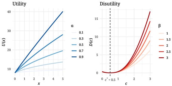
Figure 1.
Graphs of the parametric families (left) and (right) used in the numerical analysis, shown for selected parameter values and . Here, .
3.1. Emotional Parameter Sensitivity at Equilibrium: A Control-Theoretic Analysis
A control-theoretic approach allows us to determine the marginal response of the feeling and effort policies at equilibrium as the parameters and vary.
It follows from Equations (3) and (4) in optimal control theory that the optimal feeling and effort trajectories must satisfy (see [18])
Given , an equilibrium solution satisfies
Assume that the parameters are fixed. Given , suppose that is the corresponding equilibrium defined by system (15). The differentiability assumptions on the -structure imply that system (15) defines an equilibrium as differentiable functions of in a neighborhood of . This follows from differentiating (15) and observing that the matrix of the linearized system
satisfies , because of the properties of the -structure of the problem.
The marginal response of the equilibrium values with respect to variations in the sensitivity parameters is determined by the sign of the cross-derivative . Specifically, we have
Proposition 1.
Assume that the parametric -structure of the differential love game satisfies the differentiability properties specified above. Let be the equilibrium solution defined by system (15) in a neighborhood of a solution of the system. We have:
- (I)
- If , then , , and at
- (II)
- If , then , , and at .
Remark 1.
Note that, regarding the parameter dependence of the -structure, assumption in Proposition 1 is sufficient to determine the signs of , , and . This condition has a natural interpretation in terms of emotional reward: as increases, a small improvement in relationship quality, as measured by x, becomes more valuable.
Statement (I) follows from the properties of the -structure by differentiating system (15) at the point , setting to obtain
and noting that , where is defined in (16). All derivatives in the above expression are evaluated at . Statement (II) follows by a similar argument, mutatis mutandis.
According to Proposition 1, the response of the equilibrium values to small variations (with ) can be qualitatively described by the diagrams in Figure 2.
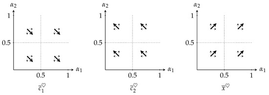
Figure 2.
Proposition 1 implies that, for fixed values of and , the gradients , , and point in the southeast, northwest, and northeast directions, respectively, at any given point .
The following proposition characterizes the marginal effects of the parameters on the equilibrium values , capturing each partner’s sensitivity to effort exertion.
Proposition 2.
Assume that the parametric -structure of the differential love game satisfies the differentiability properties specified above. Let be the equilibrium solution defined by system (15) in a neighborhood of a solution of the system. We have:
- (III)
- If , then , , and at
- (IV)
- If , then , , and at .
Similarly to the proof of Proposition 1, Statement (III) follows by differentiating system (15) at the point , now setting to obtain
and using the properties of the -structure and the fact that the matrix defined in (16) satisfies .
All derivatives in the above expression are evaluated at . Statement (IV) is obtained similarly.
Remark 2.
Condition in Proposition 2 reflects increasing marginal emotional cost with respect to : as effort sensitivity rises, the subjective burden of additional effort increases accordingly. This is a reasonable assumption and sufficient to determine the impact of on the equilibrium values.
The response of the equilibrium values to small increases in , (holding fixed) is qualitatively illustrated in Figure 3.
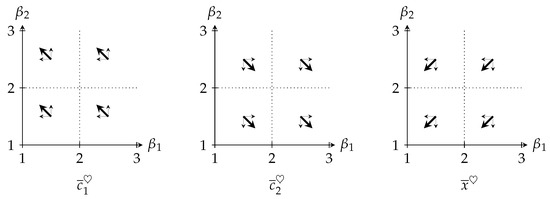
Figure 3.
Under fixed values of and , Proposition 2 implies that the gradients , , and point in the northwest, southeast, and southwest directions, respectively, across the -space.
3.2. Emotional Contour Maps at Equilibrium: Computational Feedback Analysis
In this section, we use the computational feedback model introduced in Section 2.2 to explore further how the equilibrium values in the love differential game respond to changes in the emotional sensitivity parameters and . Numerical solutions are computed using the RaBVIt-G algorithm, as previously described. While Propositions 1 and 2 establish the qualitative effects of the variation in these parameters, the feedback approach allows for a quantitative analysis once a specific -structure is defined. Additionally, it yields feedback effort maps and value functions , which are critical tools for regulating relationship dynamics. We also analyze below how variations in the parameters and affect these feedback outputs.
In our numerical analysis, we assume that heterogamy—i.e., asymmetry in the partners’ traits—affects only the emotional cost–benefit evaluation of the relationship, namely the -structure of the problem. Accordingly, we set and , where a and are fixed constants.
We will consider the following specification for the –structure of the problem:
This parametric -structure satisfies all the properties required by the model assumptions outlined in Section 2. Graphs of both parametric families, and , are presented in Figure 1. Note that the family is monotonic with respect to : for all , increases as increases. As already mentioned, the parameter captures how each partner subjectively values the quality of the relationship. Also, note that satisfies the assumption in Proposition 1, that is, the marginal emotional reward, , increases with .
Similarly, for all , the family attains an absolute minimum at and increases with for . Therefore, any effort level exceeding the preferred level is perceived as increasingly discomforting as grows. Hence, the parameter quantifies the discomfort associated with the effort gap . Also, the family satisfies the assumption in Proposition 2: the marginal emotional cost, , increases with .
Once the parametric -structure is specified, all model parameters other than and , for , are held fixed for the numerical analysis. In our study, the sensitivity parameters vary within the ranges and . All fixed parameter values and the ranges considered in the analysis are summarized in Table 1.

Table 1.
Parametric structure of the computational differential game.
The reference values for the parameters r, , , and , , as well as the range for the feeling variable , follow the plausible choices proposed in [18]. The parameter functions as a scaling factor, and the results are invariant under its rescaling. The ranges for and are selected to ensure that all theoretical modeling assumptions are satisfied. The choice of the initial condition reflects the assumption that the relationship begins at a relatively high level of feeling; accordingly, we set near the upper bound of the feasible interval for x. Variations in within a similarly high range do not affect the equilibrium configuration or the numerical results, since the stationary solutions are independent of initial conditions, as evidenced in [11].
To compute the feedback solution of the differential love game and to obtain the equilibrium value, the numerical procedure employs the RaBVIt-G algorithm outlined in Section 2, to compute the feedback solution of the differential love game and the equilibrium values , and , . The ad hoc implementation of the RaBVIt-G algorithm used in this article is available at https://github.com/jorherre/RaBVItG_LOVE/, accessed on 1 September 2025, to support reproducibility and enable sensitivity analyses under parameter changes consistent with the model’s assumptions. It builds on functions from https://github.com/jorherre/RaBVItG, accessed on 1 September 2025, which have been rewritten and adapted specifically for this work. The implementation protocol for computing equilibrium solutions is detailed in Algorithm 1 below. The computations were run on an Apple M4 processor (10-core CPU: 4 performance + 6 efficiency cores; second-generation 3 nm process; 16-core Neural Engine, ). This work required 775 RaBVIt-G runs (parameterizations), each using 16 CPU seconds, with a tolerance .
| Algorithm 1 Equilibrium Solution Computation |
|
For any given parameter set , the RaBVIt-G algorithm computes approximations to the feedback maps and , as well as the well-being (value) functions and associated with the corresponding problem.
We now present a detailed numerical sensitivity analysis. To visualize how the equilibrium solutions respond to changes in the parameters, and , we use contour plots over the corresponding parameter spaces. To enhance readability, all heatmaps in the paper employ consistent color semantics: blue represents lower values (of effort, feeling, or happiness), red represents higher values, and white denotes values close to zero. Selected contour lines are annotated with numeric labels to provide reference values. The results are discussed as they are introduced.
3.2.1. Emotional Reward Sensitivity
We first explore how the equilibrium varies with respect to the emotional reward parameters and . Controls1,Feedback summarize this analysis. In these computations, the cost parameters are fixed at , and heterogeneity between partners arises solely from variations in the parameters .
Figure 4 displays contour maps of the partners’ equilibrium effort levels and the equilibrium feeling level, for different values of . These maps show that each partner’s effort level increases with their own emotional reward parameter . Moreover, the equilibrium feeling level increases as either or increases. Since the marginal emotional reward, , grows with in this study, these effects were already established analytically in Proposition 1.
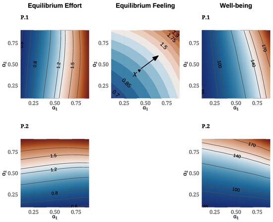
Figure 4.
Equilibrium effort level contours for both partners (left) and feeling level contours (center) are plotted over the parameter space . On the (right), a heat map of the total well-being of both partners is shown for the same parameter space, with the initial state . In these computations, the cost parameters are fixed at , so the effort cost functions in the -structure take the form for .
The cross-effects—i.e., the variation in with respect to the other partner’s parameter , —are less apparent in the contour maps. Nonetheless, Proposition 1 confirms that these cross-effects are negative. This result is further illustrated in Figure 5, which shows the feedback effort maps and the well-being functions for different values of , while keeping (and ) fixed.
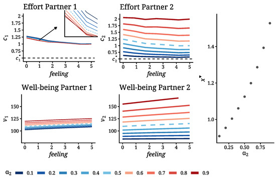
Figure 5.
Effort feedback maps (top row) and well-being (value) functions (bottom row) for different values of , with held fixed. The corresponding equilibrium feeling levels are also displayed (right). The emotional cost parameters are fixed at for these experiments.
Note that Figure 5 confirms three key insights previously suggested by the contour maps in Figure 4. First, the effort gap persists for both individuals: across all values of , each partner exerts an effort level above . Second, effort decreases as feeling increases for both individuals—that is, lower emotional closeness requires greater effort. Third, well-being increases with the initial feeling level: greater emotional closeness at the outset is associated with higher overall happiness. These features of the model were already revealed in earlier computational analyses, both in deterministic and stochastic settings. For more details, see [12] and the references therein.
The plots in Figure 5 show that, as increases, its positive effect on is significantly stronger than its negative effect on , for any given level of feeling x, in particular at the equilibrium value . Moreover, the equilibrium feeling level itself increases with .
It is worth noting that an increase in has a stronger positive effect on partner i’s equilibrium effort than the corresponding negative effect on partner j’s equilibrium effort , for any parametric -structure satisfying the conditions outlined in Section 2. This effect follows as a corollary of Proposition 1—see (17).
Corollary 1.
Under the assumptions of Proposition 1, it holds that
The well-being functions in Figure 5 show that increases in lead to higher overall happiness for both partners, although the effect is markedly stronger for partner 2. This asymmetry is confirmed numerically across the full parameter range , as illustrated in the rightmost column of Figure 4, where both partners’ well-being levels (for ) are plotted. Notably, an increase in the parameter of emotional sensitivity of a partner, , produces a greater improvement in his (her) own well-being than an equivalent increase in the parameter of the other partner, .
3.2.2. Emotional Cost Sensitivity
Next, we examine how variations in the emotional cost parameters and affect the equilibrium configuration. Figure 6 and Figure 7 summarize the analysis of sensitivity with respect to and . The reward parameters are fixed at , and asymmetry between partners arises from differences in the values and , both varying within the range .
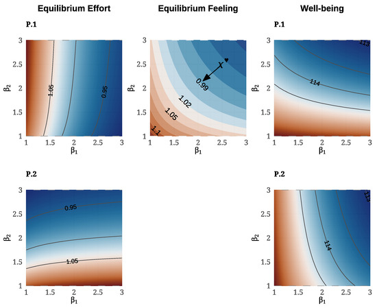
Figure 6.
Equilibrium effort level contours for both partners (left) and feeling level contours (center) are plotted over the parameter space . On the (right), a heat map of the total well-being of both partners is shown for the same parameter space, with initial state . In these computations, the reward parameters are fixed at , so the feeling reward functions in the -structure take the form for .
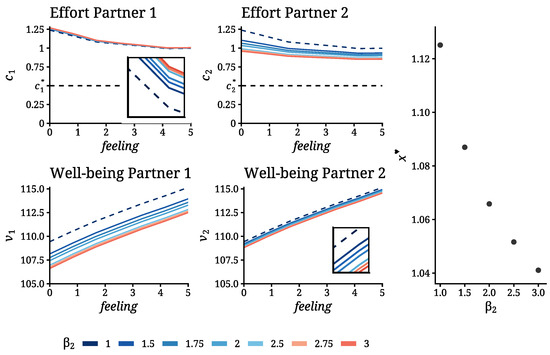
Figure 7.
Effort feedback maps (top row) and well-being (value) functions (bottom row) for different values of , with held fixed. The corresponding equilibrium feeling levels are also displayed (right). The emotional reward parameters are fixed at for these computations.
Figure 4 displays contour maps of the equilibrium effort levels and feeling level for . The plots show that each partner’s effort level, , decreases with their own emotional cost parameter, . Additionally, the equilibrium feeling level, , decreases as either or increases. As shown analytically in Proposition 2, these effects arise because the marginal emotional cost, increases with for the -structure under study.
Figure 6 shows that the cross-effects—i.e., the variation of with respect to , for —are positive. This is illustrated more clearly in Figure 7, which displays the feedback effort maps and the well-being functions for , with and held constant.
Figure 7 highlights several key features of the model’s behavior, already suggested by the contour plots in Figure 6. First, the effort gaps persist for both individuals across all values of . Second, the effort gaps decrease as the feeling increases. Third, well-being improves with higher levels of initial feeling. These properties of the model were previously identified through computational analyses in [11,12].
The plots in Figure 7, however, show that as increases, the negative effect on is substantially stronger than the positive effect on , for any x—in particular at the equilibrium value . As a result, the equilibrium feeling level decreases with . This holds for any -structure satisfying the conditions in Section 2, as a consequence of (18).
Corollary 2.
Under the assumptions of Proposition 2, it holds that
Figure 7 shows that increases in lead to lower overall happiness for both partners, and the effect is stronger for partner 1. An increase in partner i’s emotional cost parameter, , lowers his or her well-being less than that of the other partner. This asymmetry holds throughout the parameter range , as the well-being of both show in the rightmost column of Figure 6.
3.2.3. Dyadic Disparity Assessment
We further explore how the disparities between the parameters and influence the asymmetric performance of the partners at equilibrium. Figure 8 compares their respective levels of effort and well-being over the parameter range , with kept constant. The numerical analysis reveals that the partner with the higher emotional reward parameter, , exerts more effort and experiences greater well-being. As already shown in Figure 4, the equilibrium feeling level increases when either or both of the parameters increase.
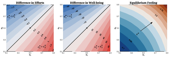
Figure 8.
Dyadic disparity at equilibrium in the -parameter space. The difference between equilibrium effort levels (left) and total well-being (center) of both partners is represented using contour maps over . On the (right), a heat map of the feeling equilibrium is shown again to provide a whole picture of the equilibrium configuration. The initial state for the computation of is , for The emotional cost parameters are fixed at .
The corresponding asymmetry analysis for the parameters and is presented in Figure 9. The contour maps display disparities in the partners’ equilibrium effort levels and well-being across the parameter domain. The computational analysis shows that the partner with the higher emotional cost parameter, , exerts less effort and experiences higher well-being. Moreover, the equilibrium feeling level decreases as either or both of the parameters increase.
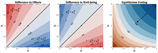
Figure 9.
Dyadic disparity at equilibrium in the -parameter space. The difference in equilibrium effort levels (left) and total well-being (center) between the two partners is illustrated using contour maps over the domain . On the (right), a heat map of the equilibrium feeling level is shown to provide a complete view of the equilibrium configuration. The initial state used for the computation of is , for . The emotional reward parameters are fixed at .
Our analysis shows that an increase in the emotional reward parameter has a greater effect on partner i’s own effort level than on that of partner j. Similarly, an increase in the emotional cost parameter influences partner i’s effort level more than partner j’s. In both cases, the resulting impact on well-being is more favorable for partner i. These findings relate to the broader question of whether one’s own traits or those of one’s partner play a greater role in determining relationship satisfaction [15]. Prior research in experimental psychology suggests that individuals’ own personality traits are more strongly associated with their own happiness [16]. Assuming that the emotional processing of rewards and costs reflects underlying personality traits, our model’s predictions are consistent with this empirical evidence.
A final disparity analysis of the equilibrium configuration, focusing on the trade-off between the two emotional sensitivity parameters, is presented in Figure 10. The analysis considers joint variations of the parameters and , while and are held constant. The contour maps show disparities in the partners’ equilibrium effort levels and well-being across the parameter domain . The results indicate that the pattern becomes more nuanced when both parameters vary simultaneously. In this case, a partner with a higher or a lower does not necessarily exert more effort. However, the numerical analysis suggests that a partner with higher consistently achieves greater well-being, regardless of their sensitivity to effort costs. As established in Proposition 1, the equilibrium feeling level decreases along the southeast direction of the domain. Notably, the increase in feeling level due to a higher is more pronounced than the increase resulting from a comparable decrease in .
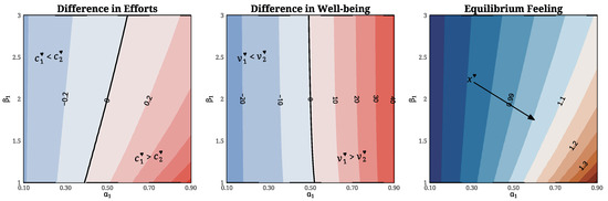
Figure 10.
Dyadic disparity at equilibrium in the -parameter space. The difference in equilibrium effort levels (left) and total well-being (center) between the two partners is shown using contour maps over the domain . On the (right), a heat map of the equilibrium feeling level is displayed to provide a complete picture of the equilibrium configuration. The initial state for the computation of is set to , for . The partner’s parameters are fixed at and .
4. Conclusions
Romantic relationships are a fundamental human experience shared across cultures. They can be understood as emotional processes that evolve over time, in which the state of the relationship is shaped by the effort each partner invests. According to relationship science, successful relationships are those that are both enduring and fulfilling in the long term. In this study, a successful relationship is modeled as a stationary Nash equilibrium of a two-person differential game, in which both partners aim to maximize their total well-being.
Life experiences and events do not carry inherent meaning; rather, they acquire significance through the interpretations of the individuals who live them. The subjective evaluation of the trade-off between emotional rewards and costs associated with a relationship plays a critical role in determining its outcome—namely, the relationship quality (or feeling level), the effort exerted by each partner, and their overall satisfaction.
Emotional rewards vary depending on individual sensitivity to relationship quality, while emotional costs arise from differences in how individuals perceive the effort required to sustain that quality. The analysis in this paper explores how the sensitivity traits defined by these two intertwined subjective processes influence relationship outcomes. Under natural psychological assumptions about these traits, our analytical results show that relationship quality improves when either partner is more sensitive to emotional rewards and also when either partner is less sensitive to emotional costs. These findings suggest that couples in which both individuals are either highly sensitive to emotional rewards or less sensitive to emotional costs tend to form more satisfying relationships and ultimately experience greater happiness.
In relationship science, the influence of one’s own traits on one’s own satisfaction is known as the actor effect, while the influence of the partner’s traits on one’s own satisfaction is referred to as the partner effect. Regarding reward sensitivity, our formal analysis shows that an individual’s effort increases with their own sensitivity but decreases with their partner’s sensitivity. Thus, the actor effect of emotional reward sensitivity on effort is positive, while the partner effect is negative. In contrast, for cost sensitivity, the actor effect on effort is negative, whereas the partner effect is positive.
The analysis also formally establishes that, in terms of effort exertion, the actor effects of sensitivity to emotional rewards and costs are stronger than the corresponding partner effects. Computational results reinforce this finding, suggesting that the differences between actor and partner effects are substantial in both cases. Moreover, the numerical analysis indicates that actor effects have a substantially more favorable impact on each partner’s overall well-being than partner effects. Notably, these results—derived from the mathematical analysis of the differential love game model—are consistent with empirical findings in social psychology: actor effects of personality traits generally exert a stronger influence on relationship satisfaction than partner effects.
While our parametric model of subjective emotional evaluation is not explicitly grounded in standard psychological personality traits, it is plausible that the two are closely related. Future research should examine how individual personality traits influence the emotional dynamics and outcomes described by the model.
The model presented in this paper incorporates flexible specifications of the utility and disutility functions—the -structure—which are consistent with psychological constructs of individuals’ emotional processing. While the qualitative findings provide valuable insights into the dynamics of successful relationships, accurate numerical estimates of the -structure, along with other model parameters, using relational data would enhance the model’s practical applicability. Identifying and curating suitable datasets for empirical calibration remains, in our view, an important direction for future research.
Author Contributions
Conceptualization, J.-M.R. and J.H.d.l.C.; methodology, J.-M.R. and J.H.d.l.C.; software, J.H.d.l.C.; validation, J.-M.R.; formal analysis, J.-M.R.; investigation, J.-M.R. and J.H.d.l.C.; resources, J.-M.R. and J.H.d.l.C.; data curation, J.H.d.l.C.; writing—original draft preparation, J.-M.R. and J.H.d.l.C.; writing—review and editing, J.-M.R.; visualization, J.H.d.l.C.; supervision, J.-M.R.; project administration, J.-M.R.; funding acquisition, J.-M.R. and J.H.d.l.C. All authors have read and agreed to the published version of the manuscript.
Funding
This research was partially supported by the CEU-San Pablo G.I.R. project G25/2-05 (JHC), the UCM–Avante Services Forte project Art. 60 #615-2024, and a 2025 RCC–Harvard University Faculty Grant (JMR).
Data Availability Statement
The original data presented in the study are openly available in GitHub (version 1.0) at https://github.com/jorherre/RaBVItG_LOVE, accessed on 11 November 2025.
Acknowledgments
A preliminary version of this article was written while JMR was visiting the Department of Psychology at Harvard University. JMR thanks Dan Gilbert for his valuable insights and stimulating discussions during that time.
Conflicts of Interest
The authors declare no conflicts of interest. The funders had no role in the design of the study; in the collection, analyses, or interpretation of data; in the writing of the manuscript; or in the decision to publish the results.
References
- Coontz, S. Marriage, a History; Viking: New York, NY, USA, 2005. [Google Scholar]
- Finkel, E.J. Romantic relationships. In The Handbook of Social Psychology, 6th ed.; Gilbert, D.T., Fiske, S.T., Finkel, E.J., Mendes, W.B., Eds.; McGraw-Hill: New York, NY, USA, 2025. [Google Scholar]
- Weimann, J.; Knabe, A.; Schöb, R. Measuring Happiness: The Economics of Well-Being; The MIT Press: Cambridge, MA, USA, 2015. [Google Scholar]
- Smoch, P.J.; Schwartz, C.R. The demography of families: A review of patterns and change. J. Marriage Fam. 2020, 82, 9–35. [Google Scholar] [CrossRef] [PubMed]
- Gottman, J.M.; Murray, J.D.; Swanson, C.C.; Tyson, R.; Swanson, K.R. The Mathematics of Marriage: Dynamic Nonlinear Models; MIT Press: Cambridge, MA, USA, 2005. [Google Scholar]
- Amato, P.R.; James, S.L. Changes in Spousal Relationships over the Marital Life Course. In Social Networks and the Life Course: Integrating the Development of Human Lives and Social Relational Networks; Alwin, D.F., Felmlee, D.H., Kreager, D.A., Eds.; Springer: Cham, Switzerland, 2018; pp. 139–158. [Google Scholar]
- Strogatz, S.H. Love affairs and differential equations. Math. Mag. 1988, 61, 35. [Google Scholar] [CrossRef]
- Rinaldi, S.; Della Rossa, F.; Dercole, F.; Gragnani, A.; Landi, P. Modeling Love Dynamics; World Scientific: Singapore, 2015; Volume 89. [Google Scholar]
- Rey, J.M. A mathematical model of sentimental dynamics accounting for marital dissolution. PLoS ONE 2010, 5, e9881. [Google Scholar] [CrossRef] [PubMed]
- Pujo-Menjouet, L. Le Jeu de l’Amour Sans le Hasard. Mathématiques du Couple; Éditions des Équaters: Paris, France, 2019. [Google Scholar]
- Herrera de la Cruz, J.; Rey, J.M. Controlling forever love. PLoS ONE 2021, 16, e0260529. [Google Scholar] [CrossRef] [PubMed]
- Herrera de la Cruz, J.; Rey, J.M. A computational stochastic dynamic model to assess the rise of breakup in a romantic relationship. Math. Methods Appl. Sci. 2025, 48, 7727–7744. [Google Scholar]
- Dockner, E.J.; Jorgensen, S.; Van Long, N.; Sorger, G. Differential Games in Economics and Management Science; Cambridge University Press: Cambridge, UK, 2000. [Google Scholar]
- Kreuzer, M.; Gollwitzer, M. Neuroticism and satisfaction in romantic relationships: A systematic investigation of intra- and interpersonal processes with a longitudinal approach. Eur. J. Personal. 2021, 36, 149–179. [Google Scholar] [CrossRef]
- Kenny, D.A.; Kashy, D.A.; Cook, W.L. Dyadic Data Analysis; The Guilford Press: New York, NY, USA, 2006. [Google Scholar]
- Bach, K.; Koch, M.; Spinath, F.M. Relationship satisfaction and The Big Five—Utilizing longitudinal data covering 9 years. Personal. Individ. Differ. 2025, 233, 112887. [Google Scholar] [CrossRef]
- Gottman, J.M.; Silver, N. The Seven Principles for Making Marriage Work; Harmony Books: New York, NY, USA, 2015. [Google Scholar]
- Goudon, T.; Lafitte, P. The lovebirds problem: Why solve Hamilton-Jacobi-Bellman equations matters in love affairs. Acta Appl. Math. 2015, 136, 147–165. [Google Scholar] [CrossRef][Green Version]
- Rey, J.M. Sentimental equilibria with optimal control. Math. Comput. Model. 2013, 57, 1965–1969. [Google Scholar] [CrossRef]
- Whyte, M.K. Dating, Mating, and Marriage; Routledge: Oxfordshire, UK, 2018. [Google Scholar]
- Basar, T.; Olsder, G.J. Dynamic Noncooperative Game Theory; SIAM: Philadelphia, PA, USA, 1999; Volume 23. [Google Scholar]
- Bardi, M.; Capuzzo-Dolcetta, I. Optimal Control and Viscosity Solutions of Hamilton-Jacobi-Bellman Equations; Birkhäuser: Boston, MA, USA, 2008. [Google Scholar]
- Falcone, M.; Ferretti, R. Semi-Lagrangian Approximation Schemes for Linear and Hamilton-Jacobi Equations; SIAM: Philadelphia, PA, USA, 2013; Volume 133. [Google Scholar]
- Mai-Duy, N.; Tran-Cong, T. Approximation of function and its derivatives using radial basis function networks. Appl. Math. Model. 2003, 27, 197–220. [Google Scholar] [CrossRef]
Disclaimer/Publisher’s Note: The statements, opinions and data contained in all publications are solely those of the individual author(s) and contributor(s) and not of MDPI and/or the editor(s). MDPI and/or the editor(s) disclaim responsibility for any injury to people or property resulting from any ideas, methods, instructions or products referred to in the content. |
© 2025 by the authors. Licensee MDPI, Basel, Switzerland. This article is an open access article distributed under the terms and conditions of the Creative Commons Attribution (CC BY) license (https://creativecommons.org/licenses/by/4.0/).