Integrating Traditional and Deep Cues for Depth from Focus Using Unfolding Networks

Abstract

Depth from focus (DFF) is an optical, passive method that perceives the dense depth map of a real-world scene by exploiting the focus cue through a focal stack, a sequence of images captured at different focal distances. In DFF methods, first, a focus volume is computed, which represents per-pixel focus quality across the focal stack, obtained either through a conventional focus metric or a deep encoder. Depth is then recovered by different strategies: Traditional approaches typically apply an argmax operation over the focus volume (i.e., selecting the image index with maximum focus), whereas deep learning-based methods often employ soft-argmax for direct feature aggregation. However, applying a simple argmax operation to extract depth from the focus volume often introduces artifacts and results in an inaccurate depth map. In this work, we propose a deep framework that integrates depth estimates from both traditional and deep learning approaches to produce an enhanced depth map. First, a deep depth module (DDM) extracts an initial depth map from deep multi-scale focus volumes. This estimate is subsequently refined through a depth unfolding module (DUM), which iteratively learns residual corrections to update the predicted depth. The DUM also incorporates structural cues from traditional methods, leveraging their strong spatial priors to further improve depth quality. Extensive experiments were conducted on both synthetic and real-world datasets. The results show that the proposed framework achieves improved performance in terms of root mean square error (RMS) and mean absolute error (MAE) compared to state-of-the-art deep learning and traditional methods. In addition, the visual quality of the reconstructed depth maps is noticeably better than that of other approaches.

1. Introduction

Depth estimation is a fundamental component of 3D vision and underpins a wide range of applications, including 3D reconstruction, augmented reality, robotics, autonomous navigation, tracking systems, and virtual or mixed reality systems [1,2,3]. Among the various techniques available, depth from focus (DFF), also known as shape from focus (SFF), is a passive optical depth estimation technique that leverages variations in image sharpness, referred to as focus measures, across a focal stack—an ordered sequence of images captured at different focal settings—to infer scene depth. Each scene point achieves maximum sharpness at a specific focal distance, enabling depth estimation by identifying the focal plane where the point appears optimally focused [4].

In the literature, numerous DFF methods have been introduced, which can be broadly classified into traditional non-learning-based approaches [5] and learning-based techniques [6,7]. In both paradigms, the depth estimation process typically begins with the construction of a focus volume (FV), from which the final depth map is derived. Traditional methods compute the FV by applying predefined focus-measure operators (e.g., Laplacian, Tenengrad, or wavelet-based measures) to the input focal stack, and then, they estimate depth by selecting the frame index that maximizes the focus response along the focal (z) direction. While conceptually simple and computationally efficient, this discrete formulation suffers from several well-known limitations: (i) edge bleeding at object boundaries due to abrupt depth transitions, (ii) loss of fine structural details because handcrafted focus measures lack representational richness, and (iii) degraded performance in complex or textureless regions where focus operators fail to provide reliable responses [5]. These shortcomings restrict the applicability of traditional SFF in real-world scenarios, particularly for scenes with challenging illumination or low-contrast textures. In contrast, learning-based approaches employ convolutional neural networks (CNNs) or encoder–decoder architectures to learn discriminative focus features directly from data. Instead of relying on handcrafted measures, these methods compute a deep FV representation and regress the final 2D depth map from the 3D FV, often using a soft-argmax operation for continuous depth prediction [8,9].

Despite outperforming traditional methods in terms of accuracy, robustness, and generalization [10], current learning-based approaches still face notable limitations. Most deep models, including [6,11,12], focus on enriching the deep focus volume, yet depth is ultimately regressed through a soft-argmax or by applying a $1\times 1$ convolution, which collapses the 3D volume into a 2D depth map. Moreover, these methods generally lack explicit depth refinement or enhancement mechanisms. As a result, the predicted depth maps may exhibit boundary artifacts, local inconsistencies, and loss of fine structural details that become more pronounced when the models are applied to real-world datasets with significant domain shifts. In addition, deep models rely solely on features extracted from the input images via convolutional networks and do not leverage prior knowledge from traditional DFF methods. For example, depth maps derived directly from the focus volume contain valuable depth cues that could be used to further enhance the final depth estimation, yet these cues are typically ignored in current learning-based approaches.

In this work, we propose a deep unfolding framework that combines the strengths of both traditional and learning-based approaches to produce enhanced depth maps. Specifically, a deep depth module (DDM) first generates an initial depth estimate from multi-scale focus volumes extracted from the input focal stack. This preliminary estimate is subsequently refined by a depth unfolding module (DUM), which iteratively learns residual corrections to progressively improve the depth prediction. Notably, the DUM incorporates structural cues from traditional methods, leveraging their strong spatial priors to enforce sharper boundaries and greater geometric consistency. The iterative refinement stage contributes in two ways: It progressively improves the depth estimates and simultaneously provides useful feedback during training, allowing the model to adjust its weights in a more informed and stable manner. Extensive experiments on both synthetic and real-world datasets demonstrate that our approach consistently outperforms state-of-the-art conventional and learning-based methods, achieving higher accuracy, sharper reconstructions, and improved generalization across diverse focal conditions. The key contributions of this paper are summarized as follows:

• We propose a deep framework for depth from focus that integrates both traditional and learning-based depth cues, enabling more accurate and robust depth estimation.
• We construct an aggregated deep focus volume by combining multi-scale feature volumes extracted through an encoder–decoder network, effectively capturing both fine details and global contextual information from the focal stack.
• We introduce a lightweight deep model within a depth unfolding module to iteratively refine the initial depth estimate, resulting in sharper boundaries, fewer artifacts, and improved generalization across diverse focal conditions.

The remainder of this paper is organized as follows: Section 2 provides a detailed background and discusses related work on depth-from-focus techniques. Section 3 introduces the proposed method, describing its key components and implementation details. Section 4 outlines the experimental setup and presents both qualitative and quantitative results to evaluate the performance of the proposed approach. Finally, Section 5 summarizes and concludes this study.

2. Background

Depth estimation is a fundamental task in computer vision applications, enabling machines to perceive and interpret the 3D structure of real-world scenes from 2D images. Accurate depth maps are vital for various applications, including autonomous driving, robotic navigation, industrial automation, augmented reality experiences, and 3D visual perception [1]. Depth estimation techniques can broadly be categorized into active and passive methods. Active methods [13] project known patterns or signals into the environment and analyze their reflections to infer depth; common examples include structured light systems and time-of-flight sensors. In contrast, passive methods estimate depth by analyzing visual information directly from images without the need for additional signals. Among passive approaches, stereo matching and structure from motion are well established, while monocular depth estimation from a single image has recently gained prominence, achieving remarkable progress [14].

Among various passive depth estimation techniques, DFF estimates depth by analyzing the sharpness of objects across a set of images captured at varying focus distances. Specifically, a sequence of images is acquired by adjusting the camera’s focus setting. According to the thin lens law, there exists a one-to-one correspondence between the maximally focused image patch and the depth of the corresponding scene point. Consequently, precise measurements of pixel-level sharpness are critical for DFF-based depth estimation [5]. Existing DFF methods can be broadly divided into two categories: (1) traditional methods and (2) deep learning-based methods.

2.1. Traditional Methods

The traditional DFF methods follow several steps, as illustrated in Figure 1. First, a set of differently focused images, commonly referred to as a focal stack, is captured. This can be achieved in multiple ways: by translating the object toward the camera, by moving the imaging device toward the object, or by adjusting the camera’s focus mechanically or electronically while keeping both the object and camera fixed in position [15].

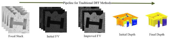
Figure 1. Steps in traditional depth-from-focus methods.

In the second step, the focus quality of each pixel in the focal stack is computed, directly impacting the accuracy of the final depth map. A focus measure (FM) operator [16] estimates pixel sharpness across the sequence, producing a three-dimensional focus volume (FV) with the same dimensions as the focal stack. FM performance depends on factors such as image content, saturation, contrast, texture, noise, window size, and the imaging device [17]. These factors can introduce artifacts and inconsistencies, with neighboring pixels of uniform depth showing large focus variations, leading to reconstruction errors. Improving FM reliability is therefore crucial.

In the DFF literature, various optimization and filtering techniques have been proposed to improve the initial FV. Subbarao and Choi [18] introduced a method that fits a planar focused image surface (FIS) to initial depth estimates from traditional approaches. Common filtering strategies include linear filtering, which averages focus measurements within a local neighborhood [15], and non-linear methods like anisotropic diffusion [19], which better preserve edges and fine structures. However, these methods rely solely on the initial FV, optimizing it in a purely data-driven manner without leveraging structural priors or additional scene information. More recent approaches integrate guidance and regularization [5,20,21], using structural cues or auxiliary information to produce more reliable depth estimates, especially in textureless regions, discontinuities, or noisy scenarios.

Once an improved FV is obtained, an initial depth map is generated by selecting, for each pixel, the image index with the highest focus response. However, this map often suffers from edge bleeding, loss of fine details, and inaccuracies in complex or low-texture regions, highlighting the need for a refinement stage that corrects local errors and enforces structural consistency. This post-processing step updates the initial depth map. Moeller et al. [22] proposed a variational DFF framework using isotropic total variation regularization. Li [23] introduced adaptive weighted guided image filtering (AWGIF) to enhance depth details. More recently, Danismaz et al. [24] improved outlier robustness via linearized least-squares Laplace regression, and Ashfaq et al. [25] presented a dual-stage focus measure approach for more reliable depth estimation.

2.2. Deep Learning-Based Methods

Deep learning-based DFF approaches estimate depth from a focal stack in two main stages: (i) constructing a deep focus volume and (ii) deriving the depth map from this volume (Figure 2). In the first stage, deep focus features are extracted using encoder–decoder (ED) networks, with both 2D and 3D architectures employed [6,8,11]. In 2DED models, each image is processed independently with 2D convolutions, and the resulting feature maps are combined to form the deep focus volume. Hazirbas et al. [8] used a VGG-16-based encoder with a mirrored decoder. DefocusNet [26] generates a focal stack from a single image via a 2DED network, followed by a second 2DED network for depth prediction. Yang et al. [6] extracted multi-scale focus volumes using a 2D CNN and applied a z-axis gradient to compute differential focus volumes, later extended with PSF-based aberration correction [9]. Fujimura et al. [7] proposed a camera-parameter-independent 2D CNN method to compute a cost volume, while Jiang et al. [27] leveraged an event-based focal stack with an attention-augmented 2DED model for multi-scale deep focus volumes. In contrast, 3DED models apply 3D convolutions to the entire focal stack, producing a volumetric representation that encodes spatial and focus information simultaneously. Wang et al. [11] introduced Inception3D, a 3D encoder–decoder generating deep focus volumes directly from the stack. Won et al. [10] combined 2D and 3D convolutions to produce multi-scale volumes, enhanced with a sharpness region detection (SRD) module. Xie et al. [28] fused the stack into an all-in-focus image via a 3D CNN, from which depth was inferred. Recently, Kang et al. [29] integrated a transformer with an LSTM–CNN decoder, enabling generalization to variable stack lengths and leveraging pretraining on large monocular depth datasets.

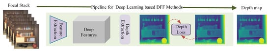
Figure 2. Pipeline for deep learning-based depth from focus methods.

For depth extraction from the deep focus volume, simple $1\times 1$ convolutions, as in [8], have limited effectiveness. Traditional $argmax$ cannot be applied directly in neural network-based methods due to its non-differentiable nature, which prevents gradient-based learning. To overcome this, a soft $argmax$[30] is commonly used, where softmax is applied along the focus dimension to produce probabilities, and the final depth is computed as the weighted sum of focus distances. Wang et al. [11] applied this operation for both depth and all-in-focus image prediction. Yang et al. [6] incorporated uncertainty confidence while applying soft $argmax$ on refined volumes. Won et al. [10] aggregated multi-scale depth maps using soft $argmax$, whereas Jiang et al. [27] used a $1\times 1$ convolution at each scale followed by fusion of the depth maps. Ganj et al. [31] further enhanced depth details by integrating priors from single-image depth estimation techniques.

For depth extraction from the deep focus volume, simple $1\times 1$ convolutions [8] are limited in effectiveness. Traditional $argmax$ is non-differentiable and unsuitable for neural networks, so soft $argmax$[30] is commonly used: A softmax along the focus dimension produces probabilities, and the final depth is computed as a weighted sum of focus distances. Wang et al. [11] applied this for both depth and all-in-focus image prediction. Yang et al. [6] incorporated uncertainty confidence on refined volumes. Won et al. [10] aggregated multi-scale depth maps using soft $argmax$, while Jiang et al. [27] combined $1\times 1$ convolutions with multi-scale depth fusion. Ganj et al. [31] further enhanced depth by integrating priors from single-image depth estimation.

3. Proposed Framework

Let the input focal stack (FS) be denoted by $\mathbf{I}\in {\mathbb{R}}^{Z\times c\times H\times W}$ consisting of Z color images, each having size $H\times W$, such that ${\mathbf{I}}_z^{\left(c\right)}(x,y)$ represents the intensity in the $z_{th}$ image at pixel location $(x,y)$ for color channel $c\in \{R,G,B\}$. The proposed framework for DFF takes the focal stack $\mathbf{I}\in {\mathbb{R}}^{Z\times c\times H\times W}$ as input to compute the improved final depth map $D\in {\mathbb{R}}^{1\times H\times W}$. The method comprises three main modules: traditional depth module (TDM), deep depth module (DDM), and depth unfolding module (DUM). First, TDM and DDM take the focal stack $\mathbf{I}$ and compute depth maps $D_t\in {\mathbb{R}}^{1\times H\times W}$ and $D_m\in {\mathbb{R}}^{1\times H\times W}$, respectively. Then, DUM integrates the depth maps $D_t$ and $D_m$ iteratively to unfold the final depth map D. The architecture of the proposed framework for SFF is depicted in Figure 3.

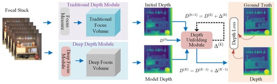
Figure 3. Overview of the proposed framework: The proposed network takes a focal stack $\mathbf{I}\in {\mathbb{R}}^{Z\times 3\times H\times W}$. The deep depth and traditional depth modules compute deep and traditional depths, which are provided to the depth unfolding module that yields the final depth $D\in {\mathbb{R}}^{1\times H\times W}$.

3.1. Traditional Depth Module

First, the focus quality for each pixel in FS is determined by applying an FM operator for each pixel in the focal stack $\mathbf{I}$. This is achieved by convolving an FM operator with the image sequence, which provides a focus value of a pixel at $(x,y)$:

$${\mathbf{F}}_z^{\left(FM\right)}(x,y)={\mathbf{I}}_z(x,y)\otimes FM,$$

(1)

where ${\mathbf{I}}_z^{\left(FM\right)}(x,y)$ denotes the traditional focus volume, ⊗ is the convolution operator, and $FM$ represents a suitable FM operator.

In the literature, a large number of FM operators have been proposed, and each FM operator exhibits some strengths and weaknesses [17]. A well-known and commonly used FM operator is the variance in image gray levels (GLVs), which computes the focus value as follows:

$${\mathbf{F}}_z^{\left(GLV\right)}(x,y)={\displaystyle \frac{1}{\left|\mathcal{N}\right|}}\sum _{(i,j)\in \mathcal{N}(x,y)}{\left(I_z(i,j)-\mu \right)}^2,$$

(2)

where $\mu$ and $\left|\mathcal{N}\right|$ are the mean gray level and total number of pixels in the small neighborhood window $\mathcal{N}$ centered at $(x,y)$, respectively. Another popular FM operator is the modified Laplacian (ML) [15], which computes the focus value for a pixel as

$${\mathbf{F}}_z^{\left(ML\right)}(x,y)=\left|{\displaystyle \frac{{\partial }^2{I}_z(x,y)}{\partial x^2}}\right|+\left|{\displaystyle \frac{{\partial }^2{I}_z(x,y)}{\partial y^2}}\right|,$$

(3)

where the first and second terms on the right-hand side are the absolute values of second-order derivatives in the x and y-dimensions, respectively. One more famous FM operator is Tenengrad (TEN), which computes the sharpness level as follows:

$${\mathbf{F}}_z^{\left(TEN\right)}(x,y)=|G_x\otimes I_z(x,y)| + |G_y\otimes I_z(x,y)|,$$

(4)

where $G_x$ and $G_y$ are the Sobel operators in the x and y-directions, respectively.

It is to be noted that our proposed method is not specific to any particular choice of FM operator, but it is generic, and thus, any FM operator can be utilized to compute the focus volume. In this work, we choose a modified-Laplacian (ML) focus measure operator. Once, we have a focus volume ${\mathbf{F}}_z^{\left(ML\right)}(x,y)$, we obtain depth map $D_t$ by applying the simple strategy of Winner Takes All, i.e., image numbers with the maximum focus values along the optical axis are taken as the depth value such that

$$D_t(x,y)=\underset{z}{\arg \max }\left\{{\mathbf{F}}_z^{\left(ML\right)}(x,y)\right\}.$$

(5)

3.2. Deep Depth Module

The deep focus module (DFM) first computes a deep focus volume ${\mathbf{G}}_z(x,y)$ from the input focal stack $\mathbf{I}$. This volume provides a per-pixel estimate of the focus level at different focal depths. It shares the same spatial resolution as the focal stack, and its number of frames equals the number of images in the stack. The module can be expressed as follows:

$$\mathbf{G}=\mathrm{DFM}(\mathbf{I},{\Theta }_1),$$

(6)

where ${\Theta }_1$ denotes the set of trainable parameters. Within the deep focus module (DFM), either 2D or 3D encoders can be employed to extract deep features. In this work, we adopt a ResNet-18 encoder [32] applied to the input focal stack to generate a feature volume pyramid. The use of multiscale features enables the model to capture both fine-grained local details and broader contextual information, thereby improving the accuracy and robustness of depth estimation. Specifically, the encoder constructs a feature pyramid ${\mathbf{H}}_l\in {\mathbb{R}}^{C_l\times H_l/f\times W_l/f}$ for $1\le l\le L=4$, where H, W, and C represent the height, width, and number of channels of the l-th hierarchical feature volume, respectively, and f denotes the downsampling factor. By selecting outputs with $f\in 4,8,16,32$, corresponding to different downsampling strides relative to the input focal stack, a multiscale feature pyramid is obtained.

$$\{{\mathbf{H}}_1,{\mathbf{H}}_2,{\mathbf{H}}_3,{\mathbf{H}}_4\}=\mathrm{ResNet}\left(\mathbf{I}\right).$$

(7)

In the decoder, each feature from the pyramid is processed by a decoder block $\left(\mathrm{DB}\right)$, which comprises a series of operations including 3D convolutions with kernel size $(3\times 3\times 3)$, 3D pooling, and batch normalization. Applying DB, followed by up-sampling (↑) and concatenation ($cat$) operations, yields the corresponding feature pyramid:

$$\left\{\begin{array}{c}{\widehat{\mathbf{H}}}_4=\mathrm{DB}\left({\mathbf{H}}_{\mathbf{4}}\right)\hfill \\ {\widehat{\mathbf{H}}}_3=\mathrm{DB}\left(cat({\mathbf{H}}_{\mathbf{3}},{\widehat{\mathbf{H}}}_4\uparrow )\right)\hfill \\ {\widehat{\mathbf{H}}}_2=\mathrm{DB}\left(cat({\mathbf{H}}_{\mathbf{2}},{\widehat{\mathbf{H}}}_3\uparrow )\right)\hfill \\ {\widehat{\mathbf{H}}}_1=\mathrm{DB}\left(cat({\mathbf{H}}_{\mathbf{1}},{\widehat{\mathbf{H}}}_2\uparrow )\right).\hfill \end{array}\right.$$

(8)

This top-down decoding progressively integrates coarse-to-fine semantic information while preserving spatial details from the encoder, producing a refined multi-scale feature representation. Finally, the aggregated focus volume $\mathbf{G}$ is obtained by adding all focus volumes from different scales.

$$\mathbf{G}=\sum _l{\mathbf{H}}_l,1\ge l\le L=4.$$

(9)

Once deep focus volume ${\mathbf{G}}_z(x,y)$ is obtained, the depth map can be computed by maximizing focus measures along the Z dimension. For this purpose, the soft argmax operation [30] is applied, which can be expressed as

$$D_m(x,y)=\sum _{z}z\times {\sigma }_z\left({\mathbf{G}}_z(x,y)\right),$$

(10)

where ${\sigma }_z(.)$ is the softmax operation along the z-dimension. This soft-argmax operation is fully differentiable and allows us to train and regress depth estimates.

3.3. Depth Unfolding Module

Now, we are given two initial depth maps, $D_m$ and $D_t$, obtained from the deep model and the traditional SFF methods, respectively. Our goal is to produce a refined depth map D that combines both sources and satisfies spatial consistency priors. We define an energy functional:

$$\begin{array}{cc}\hfill \mathcal{F}\left(D\right)& =f\left(D\right)+\lambda R\left(D\right)\lambda >0,\hfill \end{array}$$

(11)

$$\begin{array}{cc}\hfill & ={\displaystyle \frac{{\lambda }_1}{2}}\parallel D-D_m{\parallel }_2^2+{\displaystyle \frac{{\lambda }_2}{2}}{\parallel D-D_t\parallel }_2^2+R\left(D\right),{\lambda }_1,{\lambda }_2>0,\hfill \end{array}$$

(12)

where $f\left(D\right)$ is the data fidelity term, which is usually a smooth term; $R\left(D\right)$ is a regularization term, which is normally a non-smooth term; and $(\lambda ,{\lambda }_1,{\lambda }_2)$ are weights. Our objective is to minimize $\mathcal{F}\left(D\right)$ to obtain the optimal depth map D. The gradient ${\nabla }_{D}f\left(D\right)$ of $f\left(D\right)$, which denotes quadratic terms, with respect to D is computed as

$$\begin{array}{cc}\hfill f\left(D\right)& ={\displaystyle \frac{{\lambda }_1}{2}}\parallel D-D_m{\parallel }_2^2+{\displaystyle \frac{{\lambda }_2}{2}}{\parallel D-D_t\parallel }_2^2\hfill \end{array}$$

(13)

$$\begin{array}{cc}\hfill {\nabla }_{D}f\left(D\right)& ={\nabla }_D\left(\frac{{\lambda }_1}{2}\parallel D-D_m{\parallel }_2^2+\frac{{\lambda }_2}{2}{\parallel D-D_t\parallel }_2^2\right)\hfill \end{array}$$

(14)

$$\begin{array}{cc}\hfill & =({\lambda }_1+{\lambda }_2)D-({\lambda }_1{D}_m+{\lambda }_2{D}_t).\hfill \end{array}$$

(15)

A simple gradient descent step with step size $\eta >0$ becomes

$$\begin{array}{cc}\hfill D^{(k+1)}& =D^{\left(k\right)}-\eta \left(({\lambda }_1+{\lambda }_2)D^{\left(k\right)}-({\lambda }_1{D}_m+{\lambda }_2{D}_t)+\nabla R\left(D^{\left(k\right)}\right)\right)\hfill \end{array}$$

(16)

$$\begin{array}{cc}\hfill & =\left(1-\eta ({\lambda }_1+{\lambda }_2)\right)D^{\left(k\right)}+\eta ({\lambda }_1{D}_m+{\lambda }_2{D}_t)-\eta \nabla R\left(D^{\left(k\right)}\right),\hfill \end{array}$$

(17)

$$\begin{array}{cc}\hfill & =A^{\left(k\right)}-\eta \nabla R\left(D^{\left(k\right)}\right)\hfill \end{array}$$

(18)

where

$$A^{\left(k\right)}=\left(1-\eta ({\lambda }_1+{\lambda }_2)\right)D^{\left(k\right)}+\eta ({\lambda }_1{D}_m+{\lambda }_2{D}_t)$$

(19)

Now, for non-smooth regularizers $R\left(D\right)$, the update can be expressed using the proximal-gradient method:

$$D^{(k+1)}={prox}_{\eta R}\left(A^{\left(k\right)}\right),$$

(20)

where ${prox}_{\eta ,R}$ is the proximal operator associated with $R(.)$, which implicitly enforces spatial consistency and smoothness priors. Instead of using an analytical function for computing the proximal step, it is replaced with a learnable mapping $p_{{\Theta }_2}(.)$ that models both regularization and data correction:

$$\begin{array}{c}\hfill D^{(k+1)}=D^{\left(k\right)}+p_{{\Theta }_2}\left(D^{\left(k\right)},D_m,D_t\right)\end{array}$$

(21)

The term $p_{{\Theta }_2}(.)$ can further be decomposed into data term correction and proximal regularization:

$$p_{{\Theta }_2}\left(D^{\left(k\right)},D_m,D_t\right)=\eta \left[{\lambda }_1(D_m-D^{\left(k\right)})+{\lambda }_2(D_t-D^{\left(k\right)})\right]+g_{{\Theta }_2}\left(D^{\left(k\right)},D_m,D_t\right),$$

(22)

where $g_{{\Theta }_2}(.)$ approximates the proximal correction term $-\eta \nabla R\left(D^{\left(k\right)}\right)$ only, thereby learning spatial priors directly from data. Then, the update rule can be expressed as

$$\begin{array}{cc}\hfill D^{(k+1)}& =A^{\left(k\right)}+g_{{\Theta }_2}\left(D^{\left(k\right)},D_m,D_t\right)\hfill \end{array}$$

(23)

$$\begin{array}{cc}\hfill & =A^{\left(k\right)}+\Delta D\hfill \end{array}$$

(24)

$$\begin{array}{cc}\hfill \because \Delta D& =g_{{\Theta }_2}\left(D^{\left(k\right)},D_m,D_t\right)\hfill \end{array}$$

(25)

where $\Delta D$ is the residual term learned through the deep unfolding network module with parameter ${\Theta }_2$. It computes corrections for regularization by taking deep depth $D_m$, traditional depth $D_t$, and the predicted depth D as input. Note that the corrections for the data term are carried out through $A^{\left(k\right)}$. By combining both steps, the overall iterative fusion scheme can be summarized as follows:

$$\begin{array}{cc}\hfill A^{\left(k\right)}& =\left(1-\eta ({\lambda }_1+{\lambda }_2)\right)D^{\left(k\right)}+\eta \left({\lambda }_1{D}_m+{\lambda }_2{D}_t\right),\hfill \end{array}$$

(26)

$$\begin{array}{cc}\hfill D^{(k+1)}& =A^{\left(k\right)}+g_{\Theta }\left(D^{\left(k\right)},D_m,D_t\right),k=0,\dots ,K-1.\hfill \end{array}$$

(27)

In the proposed method, the predicted depth is initialized by taking the average depth from the deep and traditional depths as

$$D^{\left(0\right)}={\displaystyle \frac{D_m+D_t}{2}}.$$

(28)

We employ a lightweight deep neural network (inspired by [33]) for $f_{{\Theta }_2}(D^{\left(k\right)},D_m,D_t)$, as shown in Figure 4. Its architecture encompasses five convolutional layers; the first four are equipped with 16 filters, each kernel being $3\times 3$ and utilizing ReLU activation functions, while the last layer does not employ an activation function. This setup is specifically designed to facilitate localized adjustments. This simple model is not only effective but also efficient, comprising a mere 28,929 trainable parameters and requiring only 128.61 MB of memory for one forward/backward pass. A more sophisticated architecture may provide slightly better results.

Figure 4. Depth unfolding module: It takes deep depth $D_m\in {\mathbb{R}}^{1\times H\times W}$ and traditional depth $D_t\in {\mathbb{R}}^{1\times H\times W}$, along with the initial depth $D_0\in {\mathbb{R}}^{1\times H\times W}$, and computes depth corrections (residual depth), $\Delta$. The final refined depth $D\in {\mathbb{R}}^{1\times H\times W}$ is obtained by adding depth corrections at each iteration.

3.4. Loss Function

In the proposed framework, two modules, DDM and DUM, contain trainable parameters. The optimal parameters are obtained by minimizing the mean squared error (MSE) between the predicted depth map D and the ground truth depth map $D^{\prime }$ as follows:

$$\mathcal{L}(\mathcal{D},{\mathcal{D}}^{\prime })={\displaystyle \frac{1}{N}}\sum _{n=1}^N{\left(D^{\prime }-D\right)}^2,$$

(29)

where $(N=H\times W)$ is the resolution of the depth map: that is, the total number of pixels in a frame from the focal stack.

4. Results and Discussions

4.1. Experimental Setup

In our experiments, we evaluated the performance of the proposed method on diverse datasets that include both synthetic and real-world scenarios. The first dataset, FlyingThings3D (FT) [34], is a large-scale synthetic benchmark commonly used for depth estimation evaluation. It contains 1000 training focal stacks and 100 testing focal stacks, each comprising 15 focus-varying color images. The focal distances in this dataset are uniformly distributed between 10 and 100 units, providing a controlled and consistent setup for both training and evaluation. The second dataset, focus on defocus (FOD) [12], is another synthetic dataset that consists of 500 focal stacks, each containing five images with a resolution of $256\times 256$. Among these, 400 stacks are used for training, and 100 are used for testing. The focal distances for the images are $\{0.1,0.15,0.3,0.7,1.5\}$ units. The third dataset, Middlebury (MB) [35], is a real-world dataset used for evaluating generalization ability. It consists of 15 focal stacks, each containing 15 images, and it is used exclusively for testing. To ensure consistency, all images of MB were resized to $512\times 512$. The model was implemented in PyTorch [36] and optimized using the Adam optimizer [37] with ${\beta }_1=0.9$ and ${\beta }_2=0.999$. Training on both FT and FOD was performed with a patch size of $256\times 256$. A batch size of 1 was used throughout, corresponding to 15 focus-varying images per batch for FT and 5 focus-varying images for FOD. For evaluation on FT, the model was trained exclusively on the FT training split. For FOD, the model was also trained on its dedicated training split. For generalization to MB, we directly used the model weights trained only on the FT dataset. When referring to results from individual focal stacks in the experiments and figures, focal stack numbering follows a zero-based index (that is, the first focal stack is indexed as 0).

In addition, we evaluated the performance of the proposed model quantitatively using a comprehensive set of metrics, including mean absolute error (MAE), mean squared error (MSE), root mean squared (RMS) error, logarithmic RMS (logRMS), relative absolute error (AbsRel), relative squared error (SqRel), and accuracy thresholds Acc_1, Acc_2, and Acc_3, as defined in [8]. In addition, Pearson correlation (Corr) was also employed to assess the strength of the linear correlation between the predicted and ground truth depth maps. The higher values for metrics Corr, Acc_1, Acc_2, and Acc_3 indicate better performance, whereas lower values for the metrics MAE, MSE, RMS, logRMS, AbsRel, and SqRel mean better performance.

4.2. Ablation Study

The proposed model integrates deep and traditional depth cues to generate enhanced depth maps using the concept of unfolding networks. This integration enables the model to exploit the complementary strengths of both approaches: The deep module effectively captures complex spatial patterns from the focal stack data, while traditional depth estimation provides strong structural priors that guide and refine the learning process. Output maps obtained from the deep model and the traditional approach on the FT test dataset are shown in Figure 5. Although the traditional depth may include noise or artifacts, its inherent geometric consistency helps improve the deep predictions, leading to more accurate and stable depth maps. It is also observed that the unfolded and deep output maps appear visually similar, as the deep module progressively adapts its parameters to align with the structural constraints introduced by the unfolding mechanism. However, upon closer inspection, when zooming in, the unfolded outputs exhibit smoother object boundaries and more refined transitions, indicating improved reconstruction quality compared to the deep outputs.

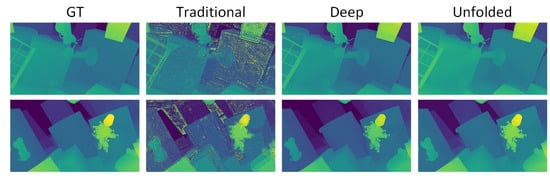
Figure 5. Visualization of output maps at different stages. The first column shows the ground truth, the second shows the deep output map, the third shows the traditional output map, and the last shows the unfolded map. Rows correspond to outputs from different samples.

The unfolding process refines the predicted outputs by iteratively adding corrections obtained from the depth unfolding module (DUM) at each step. The visual results for different iteration counts are shown in Figure 6. It can be observed that the model, trained for three iterations, produces progressively improved outputs up to the third iteration, with reduced artifacts and sharper structural details. However, beyond the third iteration, the results start to degrade slightly. This degradation occurs because the model begins to overfit with respect to the intermediate corrections, causing minor loss of fine details and introducing subtle inconsistencies across smooth regions.

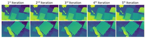
Figure 6. Qualitative results on the FT dataset after different numbers of iterations. Columns represent different iteration counts, while rows correspond to outputs from different samples.

The quantitative results for focal stack sample 1 are presented in Table 1. The results show a clear performance improvement across all six evaluation metrics, MAE, RMS, AbsRel, Acc_1, Acc_2, and Acc_3, during the initial unfolding iterations. The model, trained for three iterations, demonstrates a consistent reduction in error values and an increase in accuracy metrics up to the third iteration, indicating effective convergence and the refinement of predicted outputs. However, beyond the third iteration, a gradual decline in performance can be observed. Specifically, at the fourth and fifth iterations, the error measures begin to increase, while accuracy metrics show noticeable fluctuations. This degradation occurs because the model was optimized for three iterations; extending beyond that leads to overcorrection and the accumulation of minor prediction inconsistencies.

Table 1. Quantitative results for focal stack sample 1 from the FT dataset. Rows represent iterations, while columns denote metric evaluations at the corresponding iteration. ↑ indicates that higher values represent better performance, while ↓ indicates that lower values are better. The bold values indicate the best results.

Iteration	MAE ↓	RMS ↓	AbsRel ↓	Acc_1 ↑	Acc_2 ↑	Acc_3 ↑
1st	10.28	11.93	0.47	10.34	91.91	93.88
2nd	5.18	6.20	0.23	92.01	93.74	95.04
3rd	0.74	1.82	0.04	98.53	99.43	99.66
4th	6.82	8.39	0.22	74.16	97.44	98.18
5th	18.92	24.02	0.53	11.03	59.01	98.50

In addition, quantitative evaluations were performed on the entire FT test dataset, which consists of 100 focal stacks. The average value of each metric across all samples was computed, and the results are summarized in Table 2. The results show a consistent improvement in all evaluation metrics, MAE, RMS, AbsRel, Acc_1, Acc_2, and Acc_3, during the first three iterations, indicating that the proposed unfolding framework effectively refines the predicted outputs and enhances overall reconstruction quality. However, as observed in earlier analyses, performance begins to decline beyond the third iteration. The fourth and fifth iterations show increased error values and reduced accuracy, which can be attributed to the model being trained for three unfolding steps.

Table 2. Quantitative results for the whole test FT dataset. Rows represent the iteration, while columns denote the metric evaluation at the respective iteration. ↑ indicates that the higher values provide better performance, while ↓ indicates that the lower value is better. The bold values indicate the best results.

Iteration	MAE ↓	RMS ↓	AbsRel ↓	Acc_1 ↑	Acc_2 ↑	Acc_3 ↑
1st	17.05	21.85	0.63	4.04	82.89	88.28
2nd	9.92	13.76	0.36	81.79	88.49	92.52
3rd	3.16	6.88	0.15	95.23	98.23	99.38
4th	10.85	15.68	0.37	68.35	96.63	97.88
5th	32.66	46.02	0.81	15.11	52.76	92.48

4.3. Comparative Analysis

In this section, we compare the performance of the proposed method against both conventional and learning-based approaches. From the conventional category, we include RFVR [5], a regularization-based method, using the official implementation provided by the authors. Among learning-based baselines, we consider AiFDNet [11], for which the publicly released model weights are used. Additionally, we evaluate two variants of DFV [6]: DFV-FV, the baseline model employing a standard focus volume, and DFV-Diff, which utilizes a differential focus volume formulation to enhance feature discrimination. Furthermore, for testing on both the FT and MB datasets, we include DWild [10], a recent state-of-the-art method that jointly learns defocus and depth cues for improved prediction accuracy.

We begin our comparative analysis with the FT dataset, which serves as the largest and most comprehensive benchmark, containing 1000 training focal stacks and 100 testing focal stacks. For quantitative and qualitative evaluation, we applied all six methods: RFVR, AiFDNet, DFV-FV, DFV-Diff, DWild, and our proposed approach. The results are presented in Figure 7. The first column shows the ground truth (GT) output maps, while the remaining columns display the outputs generated by each method. Each row corresponds to results obtained from a different focal stack. As observed, RFVR yields the weakest performance, mainly due to its dependence on hand-crafted regularization and its sensitivity to the number of focal slices. In contrast, learning-based approaches produce more stable and coherent outputs across different samples. Among these, our method achieves the closest visual resemblance to the GT, particularly in reconstructing fine structural details and maintaining consistent focus across varying scene depths. Notably, in the second row, our approach more accurately reconstructs distant regions.

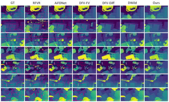
Figure 7. Qualitative comparison on the FT dataset. The columns show the GT output maps followed by the results from RFVR, AiFDNet, DFV-FV, DFV-Diff, DWild, and our method. The rows correspond to results obtained from focal stacks {4, 15, 24, 34, 54, 64, 75}.

For the overall quantitative comparison, all methods were evaluated on the complete FT test dataset consisting of 100 samples. The evaluation metrics Corr, MAE, RMS, logRMS, AbsRel, SqRel, Acc_1, Acc_2, and Acc_3 were computed using the predicted and GT output maps for each focal stack, and the average score for each metric was recorded. The results are summarized in Table 3. From the table, it is evident that our proposed method achieves the best overall performance across almost all metrics. Specifically, it attains the highest correlation score (0.98) and the lowest error values in MAE, RMS, and logRMS, indicating more accurate and stable output reconstruction. Compared to DWild, which is second best in most of the metrics, our approach reduces MAE from 5.54 to 3.16 and RMS from 10.44 to 6.87 while also improving accuracy metrics.

Table 3. Overall quantitative comparison for FT dataset. Rows represent the method employed, while columns denote the metric evaluation of the respective method. ↑ indicates that the higher values provide better performance while ↓ indicates that the lower value is better. The bold values indicate the best results.

Method	Corr ↑	MAE ↓	RMS ↓	logRMS ↓	AbsRel ↓	SqRel ↓	Acc_1 ↑	Acc_2 ↑	Acc_3 ↑
RFVR	0.73	11.89	23.63	0.79	1.55	82.66	72.79	80.81	84.60
AiFDNet	0.93	6.81	13.14	0.59	0.73	11.30	85.43	87.67	88.87
DFV-FV	0.94	6.33	12.09	0.57	0.90	27.04	85.09	87.60	89.52
DFV-Diff	0.97	5.51	10.65	0.53	0.62	7.48	86.18	88.09	89.93
DWild	0.97	5.54	10.44	0.53	0.61	7.24	86.35	88.21	89.84
Ours	0.98	3.16	6.87	0.14	0.15	12.19	95.23	98.23	99.38

Quantitative results for focal stack number 30 from the FT dataset are presented in Figure 8. All metric values are normalized to the range $[0,1]$ by dividing each measure by the maximum value of that metric across all methods, except for the accuracy metrics Acc_1 and Acc_2, which are divided by 100. The comparison includes results from AiFDNet, DFV-FV, DFV-Diff, DWild, and our proposed method. It can be observed that our approach achieves the highest performance across all shown metrics, confirming its ability to generate more accurate and consistent output maps.

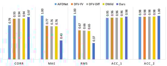
Figure 8. Quantitative comparison for focal stack number 30 from the FT dataset. The values for all measures are normalized within the range $[0,1]$. The metrics Corr, MAE, RMS, Acc_1, and Acc_2 are shown for AiFDNet, DFV-FV, DFV-Diff, DWild, and our method.

The next comparison is performed on the FOD dataset. This dataset contains only five RGB images per focal stack, which can negatively impact methods that rely heavily on the number of input images. The results are shown in Figure 9. The figure presents the qualitative results of each method. As expected, RFVR performs the weakest since its performance depends strongly on the number of focal slices, and the limited input prevents it from producing reliable outputs. The learning-based methods perform better under these constraints, demonstrating greater adaptability to limited data. Among the four depth maps shown per method, the proposed method performs slightly better qualitatively. For instance, when observing the depth map in the fourth row, other learning-based methods show regions that appear noticeably farther than in the GT, whereas the proposed method produces relatively more accurate depth estimates that better match the GT.

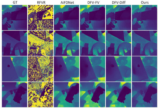
Figure 9. Comparison on the FOD dataset. The first column shows the GT depth maps, and the remaining columns show depth maps from RFVR, AiFDNet, DFV-FV, DFV-Diff, and our method, respectively. The rows correspond to the results obtained from focal stacks {7, 8, 13, 35}.

The quantitative results for focal stack 7, for which its corresponding depth maps are shown in the first row of Figure 9, are presented in Table 4. As expected, RFVR performs the weakest due to its strong dependence on the number of input images. Among the deep learning-based methods, the proposed approach achieves the best performance in four out of seven evaluation metrics. Notably, it achieves the highest correlation score of 0.912 and the lowest RMS error of 0.117, outperforming the second-best method, DFV-Diff, which obtains a correlation of 0.904 and an RMS error of 0.126. Although DFV-Diff slightly surpasses the proposed method in a few metrics, the overall quantitative results show that the proposed model performs relatively better across most of the evaluated measures.

Table 4. Quantitative comparison for focal stack number 7 from the FOD dataset, for which its corresponding qualitative results are shown in the first row of Figure 9. The rows represent different methods, while the columns denote metric evaluations for each corresponding method. The symbol ↑ indicates that higher values represent better performance, whereas ↓ indicates that lower values are better. The bold values indicate the best results.

Method	Corr ↑	MAE ↓	MSE ↓	RMS ↓	Acc_1 ↑	Acc_2 ↑	Acc_3 ↑
RFVR	0.245	0.517	0.515	0.718	18.98	32.15	43.20
AiFDNet	0.885	0.054	0.018	0.135	79.06	92.72	96.85
DFV-FV	0.891	0.062	0.016	0.128	76.69	93.93	97.46
DFV-Diff	0.904	0.054	0.016	0.126	81.98	95.11	97.10
Ours	0.912	0.063	0.014	0.117	73.57	91.22	97.49

To evaluate the generalization and effectiveness of the proposed model in real-world scenarios, the model trained on the FT dataset is applied to real objects. This setup allows us to assess how well the models perform when trained only on the 1000 training stacks of FT and then applied directly to the MB dataset without additional fine-tuning. The MB dataset consists of real-world samples and provides a pseudo-GT map captured using a structured light setup. For qualitative evaluation on the MB dataset, we applied all five methods: AiFDNet, DFV-FV, DFV-Diff, DWild, and our proposed method. Output maps were computed for each focal stack, and the results are presented in Figure 10. It can be observed that our method produces better output maps and achieves the closest resemblance to the GT, particularly in accurately reconstructing distant regions, as seen in the third row. Furthermore, in the last row, the proposed method exhibits relatively lower noise in the dusty region compared to other methods. Although DFV-FV also shows reduced noise within the dust object, it introduces noticeable background noise in this scene.

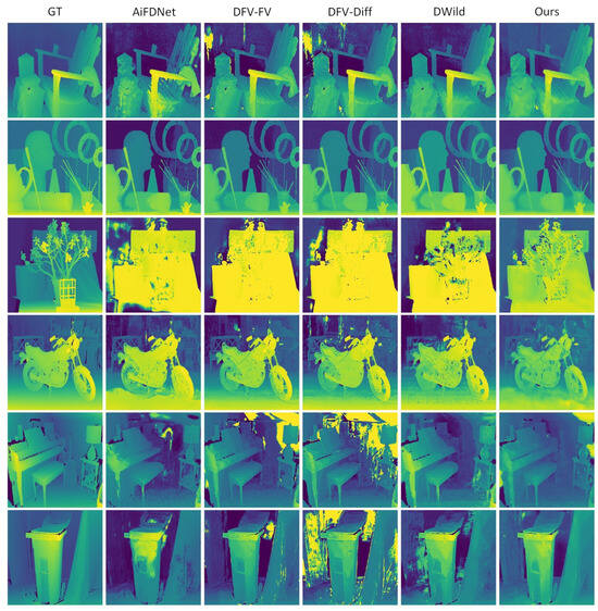
Figure 10. Qualitative comparison on the MB dataset. The columns show the GT output maps followed by the results from AiFDNet, DFV-FV, DFV-Diff, DWild, and our method. The rows correspond to results obtained from focal stacks {0, 1, 2, 3, 6, 11}.

As pseudo-GT output maps are available for the MB dataset, it is possible to quantitatively evaluate the performance of all methods. For overall comparison, each method was applied to the complete test set, and the evaluation metrics were computed using the predicted and pseudo-GT outputs for each focal stack. The average value of each metric was then calculated, and the results are summarized in Table 5. From the table, it can be observed that our proposed method achieves the highest correlation value (0.88) and the lowest MAE (4.49) among all methods, indicating improved consistency and reduced prediction error. While DWild performs competitively and shows slightly higher accuracy in some metrics, our method maintains a balanced performance across all measures. Quantitative results for focal stack 11 from the MB dataset are presented in Figure 11. All metric values are normalized to the range $[0,1]$ by dividing each measure by the maximum value of that metric across all methods, except for the accuracy metrics Acc_1 and Acc_2, which are divided by 100. The comparison includes AiFDNet, DFV-FV, DFV-Diff, DWild, and our proposed approach. It can be observed that our method achieves the best overall performance across most metrics, maintaining high correlation and low error values.

Table 5. Overall quantitative comparison for MB real-world dataset. Rows represent the method employed, while columns denote the metric evaluation of the respective method. ↑ indicates that higher values provide better performance, while ↓ indicates that the lower value is better. The bold values indicate the best results.

Method	Corr ↑	MAE ↓	RMS ↓	logRMS ↓	AbsRel ↓	SqRel ↓	Acc_1 ↑	Acc_2 ↑	Acc_3 ↑
AiFDNet	0.86	5.23	8.30	0.30	0.61	19.86	85.19	92.22	95.86
DFV-FV	0.79	5.21	9.67	0.32	0.53	14.52	85.83	91.43	94.90
DFV-Diff	0.68	6.49	11.63	0.38	0.82	32.53	80.84	87.30	91.58
DWild	0.87	4.71	8.29	0.31	0.46	11.06	88.18	92.78	95.50
Ours	0.88	4.49	7.72	0.32	0.48	11.75	87.15	93.06	95.87

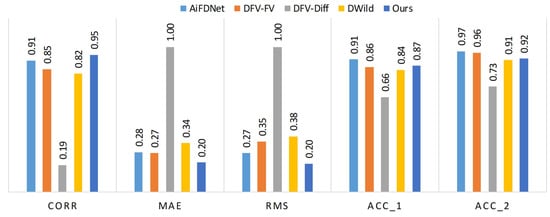
Figure 11. Quantitative comparison for focal stack number 11 from the MB dataset. The values for all measures are normalized within the range $[0,1]$. The metrics CORR, MAE, RMS, Acc_1, and Acc_2 are shown for AiFDNet, DFV-FV, DFV-Diff, DWild, and our methods.

4.4. Complexity Analysis

In this section, time complexity analysis is provided. Inference times were measured on the FOD dataset, where each input consists of a stack of five RGB images at $256\times 256$ resolution. As shown in Table 6, our method achieves a comparable runtime to existing approaches while maintaining a similar parameter count. Although DFV-FV and DFV-Diff are faster than others, AiFDNet exhibits slightly slower inference time than others. Our model provides improved accuracy with only a minor increase in computation.

Table 6. Parameter count and average inference time on FOD dataset for each evaluated method.

Method	Params (M)	Mean Time (s)
AiFDNet [11]	16.53	0.0272
DFV-FV [6]	19.5	0.0169
DFV-Diff [6]	19.5	0.0179
Ours	19.53	0.0260

4.5. Failure Case Analysis

Although the proposed framework improves depth estimation by incorporating traditional depth cues, certain limitations remain. In particular, when the depth estimated by the deep module and the cues from traditional methods differ significantly, the resulting depth map may exhibit reduced accuracy. For instance, a case of reduced accuracy is shown in Figure 12, where most deep models, including AiFDNet, DFV-FV, DFV-Diff, and DWild, fail to produce depth maps aligned with the ground truth (GT). The proposed method attempts to improve the results, but it only achieves a modest improvement. The quantitative metrics for AiFDNet, DFV-FV, DFV-Diff, DWild, and the proposed method are reported in Table 7. These metrics highlight the failure of the deep models to accurately predict depth in this case. While the proposed method shows slight improvements in Corr, MAE, RMS, and Acc_3, the final depth map still contains noticeable errors. These observations indicate that, although integrating traditional depth cues can enhance performance, the method’s effectiveness is limited in scenarios where the deep module predictions and traditional cues are highly inconsistent.

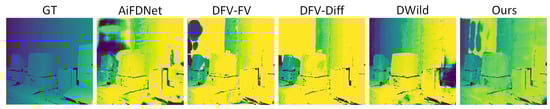
Figure 12. Qualitative comparison of a failure case from focal stack 14 from the MB dataset. The GT and results from AiFDNet, DFV-FV, DFV-Diff, and DWild are compared with our method. While none of the models fully capture the correct distance of objects from the viewpoint, our approach remains comparatively closer to the GT.

Table 7. Quantitative comparison of a failure case from focal stack 14 from the MB dataset. The bold values indicate the best results.

Method	Corr ↑	MAE ↓	RMS ↓	AbsRel ↓	Acc_1 ↑	Acc_2 ↑	Acc_3 ↑
AiFDNet	0.56	15.96	24.23	0.35	55.77	72.15	91.32
DFV-FV	0.48	16.56	24.22	0.38	56.85	69.68	89.04
DFV-Diff	0.33	18.20	25.50	0.49	53.67	65.61	84.97
DWild	0.47	15.04	27.24	0.24	71.62	81.07	90.53
Ours	0.61	14.73	22.25	0.31	64.17	79.79	91.89

5. Conclusions

In this paper, we introduced a novel framework for depth from focus that fuses insights from both traditional and deep learning-based methods to produce enhanced depth maps. The deep depth module (DDM) generates an initial estimate from multi-scale focus volumes, which is further refined by the depth unfolding module (DUM) through iterative residual updates. By integrating structural information from conventional techniques, the model enforces sharper edges and greater spatial coherence. Evaluation on both synthetic and real-world datasets shows that the proposed approach surpasses current state-of-the-art methods, providing more accurate, reliable, and generalizable depth predictions across varied focal scenarios.

References

- Zheng, Z.; Feng, S.; Chen, C.; Qu, Y. Depth from Focus in 3D Measurement: An Overview. IEEE Trans. Instrum. Meas. 2025, 74, 1–38. [Google Scholar] [CrossRef]
- Wofk, D.; Ma, F.; Yang, T.J.; Karaman, S.; Sze, V. Fastdepth: Fast monocular depth estimation on embedded systems. In Proceedings of the 2019 International Conference on Robotics and Automation (ICRA), Montreal, QC, Canada, 20–24 May 2019; IEEE: New York, NY, USA, 2019; pp. 6101–6108. [Google Scholar]
- Jiang, D.; Wang, H.; Li, T.; Gouda, M.A.; Zhou, B. Real-time tracker of chicken for poultry based on attention mechanism-enhanced YOLO-Chicken algorithm. Comput. Electron. Agric. 2025, 237, 110640. [Google Scholar] [CrossRef]
- Yan, T.; Qian, Y.; Zhang, J.; Wang, J.; Liang, J. SAS: A General Framework Induced by Sequence Association for Shape from Focus. IEEE Trans. Pattern Anal. Mach. Intell. 2025, 47, 8471–8488. [Google Scholar] [CrossRef]
- Ali, U.; Mahmood, M.T. Robust focus volume regularization in shape from focus. IEEE Trans. Image Process. 2021, 30, 7215–7227. [Google Scholar] [CrossRef]
- Yang, F.; Huang, X.; Zhou, Z. Deep depth from focus with differential focus volume. In Proceedings of the IEEE/CVF Conference on Computer Vision and Pattern Recognition, New Orleans, LA, USA, 18–24 June 2022; pp. 12642–12651. [Google Scholar]
- Fujimura, Y.; Iiyama, M.; Funatomi, T.; Mukaigawa, Y. Deep depth from focal stack with defocus model for camera-setting invariance. Int. J. Comput. Vis. 2024, 132, 1970–1985. [Google Scholar] [CrossRef]
- Hazirbas, C.; Soyer, S.G.; Staab, M.C.; Leal-Taixé, L.; Cremers, D. Deep depth from focus. In Proceedings of the Computer Vision—ACCV 2018: 14th Asian Conference on Computer Vision, Perth, Australia, 2–6 December 2018; Revised Selected Papers, Part III 14. Springer: Berlin/Heidelberg, Germany, 2019; pp. 525–541. [Google Scholar]
- Yang, X.; Fu, Q.; Elhoseiny, M.; Heidrich, W. Aberration-aware depth-from-focus. IEEE Trans. Pattern Anal. Mach. Intell. 2023, 47, 7268–7278. [Google Scholar] [CrossRef]
- Won, C.; Jeon, H.G. Learning depth from focus in the wild. In Proceedings of the European Conference on Computer Vision, Tel Aviv, Israel, 23–27 October 2022; Springer: Berlin/Heidelberg, Germany, 2022; pp. 1–18. [Google Scholar]
- Wang, N.H.; Wang, R.; Liu, Y.L.; Huang, Y.H.; Chang, Y.L.; Chen, C.P.; Jou, K. Bridging unsupervised and supervised depth from focus via all-in-focus supervision. In Proceedings of the IEEE/CVF International Conference on Computer Vision, Montreal, QC, Canada, 11–17 October 2021; pp. 12621–12631. [Google Scholar]
- Maximov, M.; Galim, K.; Leal-Taixé, L. Focus on defocus: Bridging the synthetic to real domain gap for depth estimation. In Proceedings of the IEEE/CVF Conference on Computer Vision and Pattern Recognition, Seattle, WA, USA, 14–19 June 2020; pp. 1071–1080. [Google Scholar]
- Rodrigues, R.T.; Miraldo, P.; Dimarogonas, D.V.; Aguiar, A.P. Active depth estimation: Stability analysis and its applications. In Proceedings of the 2020 IEEE International Conference on Robotics and Automation (ICRA), Paris, France, 31 May–31 August 2020; IEEE: New York, NY, USA, 2020; pp. 2002–2008. [Google Scholar]
- Schonberger, J.L.; Frahm, J.M. Structure-from-motion revisited. In Proceedings of the IEEE Conference on Computer Vision and Pattern Recognition, Las Vegas, NV, USA, 27–30 June 2016; pp. 4104–4113. [Google Scholar]
- Nayar, S.K.; Nakagawa, Y. Shape from focus. IEEE Trans. Pattern Anal. Mach. Intell. 1994, 16, 824–831. [Google Scholar] [CrossRef]
- Krotkov, E. Focusing. Int. J. Comput. Vis. 1988, 1, 223–237. [Google Scholar] [CrossRef]
- Pertuz, S.; Puig, D.; Garcia, M.A. Analysis of focus measure operators for shape-from-focus. Pattern Recognit. 2013, 46, 1415–1432. [Google Scholar] [CrossRef]
- Subbarao, M.; Choi, T. Accurate recovery of three-dimensional shape from image focus. IEEE Trans. Pattern Anal. Mach. Intell. 1995, 17, 266–274. [Google Scholar] [CrossRef]
- Mahmood, M.T.; Choi, T.S. Nonlinear approach for enhancement of image focus volume in shape from focus. IEEE Trans. Image Process. 2012, 21, 2866–2873. [Google Scholar] [CrossRef] [PubMed]
- Jeon, H.G.; Surh, J.; Im, S.; Kweon, I.S. Ring Difference Filter for Fast and Noise Robust Depth From Focus. IEEE Trans. Image Process. 2019, 29, 1045–1060. [Google Scholar] [CrossRef]
- Ali, U.; Lee, I.H.; Mahmood, M.T. Guided image filtering in shape-from-focus: A comparative analysis. Pattern Recognit. 2021, 111, 107670. [Google Scholar] [CrossRef]
- Moeller, M.; Benning, M.; Schönlieb, C.; Cremers, D. Variational depth from focus reconstruction. IEEE Trans. Image Process. 2015, 24, 5369–5378. [Google Scholar] [CrossRef] [PubMed]
- Li, Y.; Li, Z.; Zheng, C.; Wu, S. Adaptive weighted guided image filtering for depth enhancement in shape-from-focus. Pattern Recognit. 2022, 131, 108900. [Google Scholar] [CrossRef]
- Danismaz, S.; Dogan, R.O.; Dogan, H. Two-phase deep learning method for image fusion-based extended depth of focus. J. Supercomput. 2025, 81, 1–27. [Google Scholar] [CrossRef]
- Ashfaq, K.; Mahmood, M.T. A dual-stage focus measure for vector-valued images in shape from focus. Pattern Recognit. 2026, 170, 112112. [Google Scholar] [CrossRef]
- Lu, Y.; Milliron, G.; Slagter, J.; Lu, G. Self-supervised single-image depth estimation from focus and defocus clues. IEEE Robot. Autom. Lett. 2021, 6, 6281–6288. [Google Scholar] [CrossRef]
- Jiang, C.; Lin, M.; Zhang, C.; Wang, Z.; Yu, L. Learning Depth from Focus with Event Focal Stack. IEEE Sens. J. 2024, 25, 1950–1958. [Google Scholar] [CrossRef]
- Xie, X.; Qingyan, J.; Chen, D.; Guo, B.; Li, P.; Zhou, S. StackMFF: End-to-end multi-focus image stack fusion network. Appl. Intell. 2025, 55, 503. [Google Scholar] [CrossRef]
- Kang, X.; Han, F.; Fayjie, A.R.; Vandewalle, P.; Khoshelham, K.; Gong, D. FocDepthFormer: Transformer with Latent LSTM for Depth Estimation from Focal Stack. In Proceedings of the Australasian Joint Conference on Artificial Intelligence, Melbourne, VIC, Australia, 25–29 November 2024; Springer: Berlin/Heidelberg, Germany, 2024; pp. 273–290. [Google Scholar]
- Kendall, A.; Martirosyan, H.; Dasgupta, S.; Henry, P.; Kennedy, R.; Bachrach, A.; Bry, A. End-to-end learning of geometry and context for deep stereo regression. In Proceedings of the IEEE International Conference on Computer Vision, Venice, Italy, 22–29 October 2017; pp. 66–75. [Google Scholar]
- Ganj, A.; Su, H.; Guo, T. HybridDepth: Robust Metric Depth Fusion by Leveraging Depth from Focus and Single-Image Priors. In Proceedings of the 2025 IEEE/CVF Winter Conference on Applications of Computer Vision (WACV), Tucson, AZ, USA, 28 February–4 March 2025; IEEE: New York, NY, USA, 2025; pp. 973–982. [Google Scholar]
- He, K.; Zhang, X.; Ren, S.; Sun, J. Deep residual learning for image recognition. In Proceedings of the IEEE Conference on Computer Vision and Pattern Recognition, Las Vegas, NV, USA, 27–30 June 2016; pp. 770–778. [Google Scholar]
- Dong, J.; Pan, J.; Ren, J.S.; Lin, L.; Tang, J.; Yang, M.H. Learning spatially variant linear representation models for joint filtering. IEEE Trans. Pattern Anal. Mach. Intell. 2021, 44, 8355–8370. [Google Scholar] [CrossRef]
- Mayer, N.; Ilg, E.; Hausser, P.; Fischer, P.; Cremers, D.; Dosovitskiy, A.; Brox, T. A large dataset to train convolutional networks for disparity, optical flow, and scene flow estimation. In Proceedings of the IEEE Conference on Computer Vision and Pattern Recognition, Las Vegas, NV, USA, 27–30 June 2016; pp. 4040–4048. [Google Scholar]
- Scharstein, D.; Hirschmüller, H.; Kitajima, Y.; Krathwohl, G.; Nešić, N.; Wang, X.; Westling, P. High-resolution stereo datasets with subpixel-accurate ground truth. In Proceedings of the Pattern Recognition: 36th German Conference, GCPR 2014, Münster, Germany, 2–5 September 2014; Proceedings 36. Springer: Berlin/Heidelberg, Germany, 2014; pp. 31–42. [Google Scholar]
- Paszke, A.; Gross, S.; Massa, F.; Lerer, A.; Bradbury, J.; Chanan, G.; Killeen, T.; Lin, Z.; Gimelshein, N.; Antiga, L.; et al. Pytorch: An imperative style, high-performance deep learning library. Adv. Neural Inf. Process. Syst. 2019, 32, 8026. [Google Scholar]
- Kingma, D.P. Adam: A method for stochastic optimization. arXiv 2014, arXiv:1412.6980. [Google Scholar]
Disclaimer/Publisher’s Note: The statements, opinions and data contained in all publications are solely those of the individual author(s) and contributor(s) and not of MDPI and/or the editor(s). MDPI and/or the editor(s) disclaim responsibility for any injury to people or property resulting from any ideas, methods, instructions or products referred to in the content. |
© 2025 by the authors. Licensee MDPI, Basel, Switzerland. This article is an open access article distributed under the terms and conditions of the Creative Commons Attribution (CC BY) license (https://creativecommons.org/licenses/by/4.0/).