Explainable Machine Learning Financial Econometrics for Digital Inclusive Finance Impact on Rural Labor Market

Abstract

The research examines how digital inclusive finance reshapes the rural labor market using an auditable index system and an interpretable learning pipeline. We construct a four-pillar framework for the rural labor market covering labor behavior, labor structure, security and fairness, and sustainability, and compute county-level scores with an Attribute Hierarchy Model plus Fuzzy Comprehensive Evaluation (AHM–FCE). Using data for 58 counties in Jiangsu from 2014 to 2023, we estimate nonlinear links from overall and sub-dimensional digital finance to labor market outcomes with a random forest optimized by Particle Swarm Optimization plus Genetic Algorithm (PSO-GA-RF). Theoretical contribution: we provide a measurement-based bridge from digital inclusive finance to rural labor markets by aligning access, usage, and service quality with the four pillars of the rural labor market index, which yields testable county level predictions on participation, job quality, equity, and persistence of gains. Maps show heterogeneity, with higher behavior scores, lagging sustainability, and a north–south gradient. Empirically, stronger digital finance is associated with higher non-agricultural employment, better job quality, narrower urban–rural gaps, and stronger protection mechanisms, with larger effects where rural population shares and policy support are higher. Findings are robust to variable transforms, bandwidth choices, and tuning.

1. Introduction

The labor economy plays a critical role in supporting regional and economic stability. Labor is a fundamental factor of production. The labor market is a distinct segment within the broader factor market [1]. The labor economy has unique regional and temporal characteristics [2]. It significantly contributes to increasing farmers’ incomes, driving industrialization and urbanization, and absorbing surplus rural labor. These roles collectively help maintain social stability in rural areas. In 2022, the global urbanization rate reached approximately 68%. However, around 20% of the world’s population (about 1.7 billion people) still reside in underdeveloped or marginalized regions. Approximately 83% of these populations are rural residents [3]. This situation highlights the urgent need for targeted rural development strategies. Stable agricultural and rural development directly affects employment security, economic growth, and societal well-being. Therefore, addressing challenges in the rural labor market (RLM) is vital. Effective strategies can improve wage levels for rural residents, release surplus agricultural labor, and optimize labor allocation. Furthermore, these measures can accelerate agricultural modernization and labor transition to non-agricultural sectors. Ultimately, this will promote urbanization and balanced rural–urban development [4,5].

China’s rural revitalization strategy has shown significant potential but faces several critical challenges. The strategy has led to notable progress across various regional industries. This progress has boosted regional development, increased farmers’ incomes, and improved overall well-being [6]. However, the strategy remains in its early stages and continues to face obstacles. These include low agricultural productivity, an underdeveloped industrial structure, and imbalances in human resource availability and quality [7,8]. Furthermore, compound risks from market volatility, social dynamics, and environmental factors have become increasingly evident. These factors highlight urgent problems that require immediate attention [9]. In particular, the rural labor sector faces two major issues: insufficient labor supply and inadequate workforce skills. These problems have weakened the human capital base essential for developing modern agriculture in China [10]. Resolving these issues demands a comprehensive approach. This includes increasing agricultural productivity, optimizing industrial structures, and enhancing human resource capacities. Such measures are vital to ensure the sustainable advancement of China’s rural revitalization strategy. Against this backdrop, DIF provides a tractable pathway to mitigate these pressures through broader digital access, expanded credit, and support for entrepreneurship in rural areas.

Digital inclusive finance (DIF) significantly enhances access to financial services, fostering economic growth and inclusion. It fosters economic growth and inclusion through the integration of digital technologies with financial products. Compared to traditional financial models, DIF significantly reduces service costs. This cost reduction enables broader coverage, particularly for underserved populations in rural and remote areas [11,12]. As a result, DIF promotes financial inclusion and high-quality economic growth through wider participation in economic activities [13]. DIF leverages innovations such as mobile internet, big data, and cloud computing. These technologies enhance financial market efficiency, reduce transaction barriers, and address information asymmetry. Consequently, historically marginalized groups gain better access to financial resources. Studies indicate that DIF reduces income inequality [14], increases household consumption capacity [15], and promotes inclusive economic growth.

By improving access to financial resources, DIF encourages entrepreneurship and productive investments, especially among rural populations. This leads to higher household wealth accumulation and supports rural revitalization efforts. Furthermore, DIF contributes to regional green growth by financing environmentally sustainable projects, reducing carbon emissions, and stimulating green innovation [16]. In agricultural regions, DIF alleviates credit constraints. It allows farmers to invest more productively, enhancing agricultural resilience [11]. In regions facing ecological and economic challenges, such as the Yellow River Basin, DIF promotes industrial upgrading by improving factor market efficiency and encouraging innovation [17,18]. Through these mechanisms, DIF reduces financing constraints for small and medium-sized enterprises (SMEs). Thus, DIF helps overcome capital-access challenges and supports the development of critical industries [19].

Most scholars acknowledge the inclusive nature of digital finance. They suggest that DIF expands both the breadth and depth of financial services [20]. It plays an essential role in alleviating poverty by reducing financial constraints faced by vulnerable groups [21]. Existing research indicates that DIF significantly increases farmers’ incomes. This increase occurs mainly by lowering entry barriers, reducing financial exclusion, and enabling poverty alleviation [22,23,24]. From the perspectives of credit constraints and market failures, DIF benefits low-income populations. It helps overcome market inefficiencies and eases credit access [25,26]. DIF also improves financial stability by lowering service access costs for low-income groups [27]. Inclusive finance contributes to GDP growth in developing countries and raises farmers’ income levels [28]. Through timely and effective financial information [29], farmers can easily access suitable financial products via mobile phones or computers. Such convenience improves the efficiency of rural household financial portfolios and boosts property income. DIF further encourages household consumption, particularly among families with lower income and weaker financial conditions. Nevertheless, financial market instability may heighten operational risks in agriculture, disproportionately affecting disadvantaged groups [30]. Some scholars question the effectiveness of DIF in agricultural contexts. They argue that China’s DIF remains at an early development stage, limiting its short-term impact on rural economic growth. Furthermore, many farmers lack sufficient knowledge of digital financial services. This knowledge gap may unintentionally widen the income disparity between urban and rural residents.

Current research on DIF in China primarily examines macroeconomic effects in rural areas. Many studies focus on poverty alleviation and household asset allocation. However, there is limited research on DIF’s specific impacts on RLM. Existing frameworks often neglect complex interactions within Rural Labor Market. They commonly treat the relationship between DIF and rural economic performance as a “black box”. Most studies rely on traditional regression methods. These approaches offer general evaluations of economic impacts but rarely analyze effects specifically on RLM. Comprehensive evaluation systems and empirical tests based on detailed datasets are notably lacking. Advancements in big data and machine learning provide new opportunities to explore hidden data relationships. These technologies can clarify how DIF influences rural labor supply, employment structure, and income distribution. Applying these advanced techniques can address current methodological shortcomings. It enables more precise and dynamic evaluations, deepening our understanding of DIF’s role in RLM. By integrating interpretable machine learning with econometric modeling, our approach can reveal the detailed channels through which DIF shapes various labor outcomes. This approach could significantly enhance academic progress in this field.

To address the limitations of traditional econometric approaches in capturing nonlinear and regionally heterogeneous effects of DIF on rural labor outcomes, this paper defines the concept of the RLM and systematically outlines the theoretical mechanisms through which DIF influences RLM. It proposes an explainable artificial intelligence (XAI) based machine learning framework, a PSO-GA-RF model, which integrates a novel Gini–OOB feature importance measure. The main contributions of the research include systematically establishing a clear theoretical framework (“Digital Inclusive Finance–Rural Labor Market”) that captures micro-level mechanisms within the rural labor market. The proposed PSO-GA-RF approach innovatively combines PSO and GA for joint optimization of RF parameters and feature selection, enhancing model accuracy and interpretability. The integrated Gini–OOB index further evaluates feature importance comprehensively from the perspectives of purity and generalization capability. Empirical findings reveal that DIF significantly enhances the RLM by promoting non-agricultural employment and improving employment quality. Notably, the strength of these impacts exhibits clear regional heterogeneity, with more pronounced effects in northern Jiangsu. The underlying causes for such heterogeneity are discussed from multiple dimensions, including regional financial infrastructure, financing demands of rural industries, digital financial literacy, and variations in local policy support. Based on these insights, relevant policy recommendations are proposed.

This paper proceeds as follows. Section 2 reviews scholarship on the rural labor market and digital inclusive finance and motivates a four pillar RLM indicator system. Section 3 sets out the methodology, including AHM and FCE for index construction, and a PSO GA optimized random forest with a Gini and OOB based importance measure under a single objective that minimizes fivefold cross-validated MSE. Section 4 presents the data for Jiangsu counties from 2014 to 2023 and reports the main empirical results, including standardized RLM scores, core spatial patterns, and the key drivers identified by the feature importance analysis. Section 5 concludes with implications for policy and future research.

2. Literature Review

2.1. Rural Labor Market

The dependent variable in the research is a set of RLM indicators. We follow established labor economics perspectives on search and matching and on labor market resilience, which motivate a four-pillar organization that maps behavior, structure, security and fairness, and economic sustainability. These four pillars correspond to the standard margins that shape labor outcomes in economic theory: individual participation and mobility (behavior), cross-sector and cross-group allocation (structure), institutional rules and access (security and fairness), and intertemporal persistence under shocks (economic sustainability). Compared with prior studies that often proxy the rural labor market with one or two variables (e.g., employment rate, migration share, or a sectoral ratio) and compress digital inclusive finance into a single composite score, we retain four labor pillars and three DIF sub-dimensions to enable channel-specific, theory-consistent tests. This organization reduces overlap across indicators and provides a minimally sufficient coverage of both efficiency and equity margins. We define four subindices of the RLM index: the Labor Behavior Index (LBI), Labor Structure Index (LSI), Labor Security and Fairness Index (LSFI), and Labor Economic Sustainability Index (LESI). Table 1 lists the county-level indicators for each subindex.

Table 1. The Rural Labor Market indicator system.

Primary Indicator	Secondary Indicator	How Indicators Are Measured	Unit	Main Reference
Labor Behavior (X1)	Employment Scale (X11)	Rural employment population	10,000 persons	[31]
	Employment Quality (X12)	Total income of employed persons/number of employed persons	Yuan/ person	[32]
	Non-agricultural Employment Level (X13)	Total rural labor force working in non-agricultural sectors/total rural employment population	ratio	[33]
	External Migration Ratio (X14)	Number of rural laborers migrating externally/total rural employment population	ratio	[32]
Labor Structure (X2)	Urban–Rural Income Gap (X21)	Urban residents’ disposable income per capita/rural residents’ disposable income per capita	ratio	[31]
	Gender Balance (X22)	Female labor force/total labor force	ratio	[34]
	Industrial Structure Rationality (X23)	Number of employees in industrial and service sectors/number of employees in primary industries	ratio	[35]
	Aging Level (X24)	Number of laborers aged 65 and above/total labor force	ratio	[36]
Labor Security and Fairness (X3)	Public Finance Support (X31)	Fiscal expenditure/regional GDP	ratio	[37]
	Non-agricultural Income Ratio (X32)	Rural residents’ non-agricultural income/total rural residents’ income	ratio	[33]
	Labor-intensive Industry Support (X33)	Value of labor-intensive industry output/regional GDP	ratio	[32]
Labor Economic Sustainability (X4)	Agricultural Mechanization Level (X41)	Total agricultural machinery power	kW	[38]
	Employment Flow Shock (X42)	Employment ratio of the current year to the previous year	ratio	[36]
	Consumption-Driven Employment Capacity (X43)	Rural residents’ consumer spending/regional GDP	ratio	[39]

Labor Behavior Index (LBI) reflects participation, mobility, and search intensity in rural labor markets as core behavioral margins. It includes X₁₁ Employment Scale, X₁₂ Employment Quality, X₁₃ Non-agricultural Employment Level, and X₁₄ External Migration Ratio, which together describe the size and quality of local employment and the flow of workers between farm and non-farm activities. Evidence shows that migration reshapes local labor supply and land use, which validates the inclusion of an outward-migration measure [31,32]. Studies on off-farm diversification link non-farm engagement with household welfare and stability, which supports the emphasis on job quality and non-agricultural employment as markers of labor market dynamism [33]. Taken together, LBI captures the flow and intensity side of participation and matching, complementing stock-based measures in other pillars. These indicators complement each other by capturing both the stock and the flow aspects of rural labor behavior over time.

The Labor Structure pillar captures the stock and composition side, sectoral allocation and distribution across groups, which determines productivity and equity in rural economies. It includes X₂₁ Urban Rural Income Gap, X₂₂ Gender Balance, X₂₃ Industrial Structure Rationality, and X₂₄ Aging Level to track the shift from agriculture toward industry and services and the distributional profiles that accompany this shift. Land use and peri urban industrialization research documents the central role of structural transformation in rural development [31,35]. Production diversity is associated with broader welfare outcomes which motivates attention to sectoral mix and distributional gaps [34]. The aging of the rural workforce has measurable effects on resilience and productivity which justifies the inclusion of the aging indicator within the structural profile [36]. This pillar therefore complements behavior by locating where workers are allocated and how composition conditions productivity and distribution.

The Labor Security and Fairness evaluates protection and equitable access to opportunities in rural labor markets. It includes X₃₁ Public Finance Support, X₃₂ Non-agricultural Income Ratio, and X₃₃ Labor intensive Industry Support as proxies for fiscal capacity for enforcement and safety nets income diversification and local absorption capacity. Evidence on rural enterprises shows their contribution to local resilience which grounds the measurement of absorption capacity [37]. Studies on technology and rural communities warn that uneven access can lead to uneven outcomes which underlines the fairness orientation of this index [32,33]. By focusing on rules, protection, and access, this pillar links financial and institutional capacity to who can participate and benefit, addressing the equity margin that prior frameworks often treat only implicitly. The indicators form a coherent set that captures institutional support livelihood diversification and job creation capacity.

The Labor Economic Sustainability gauges the persistence of gains and resilience to shocks in rural labor outcomes. It includes X₄₁ Agricultural Mechanization Level, X₄₂ Employment Flow Shock, and X₄₃ Consumption Driven Employment Capacity to represent modernization stability and demand side support. Demographic and sectoral trends highlight the need for mechanization as a response to tightening rural labor supply and as a marker of modernization [38]. Aging-related evidence links workforce composition to resilience which supports the use of flow stability as a sustainability signal [36]. Local enterprise activity and consumption linkages are recognized components of community resilience which motivates the demand driven employment indicator [39]. This pillar closes the dynamic dimension by measuring whether improvements in behavior, structure, and fairness are maintained over time and under shocks.

In summary, the four pillars collectively cover behavior (flows), structure (stocks), security and fairness (rules and access), and sustainability (persistence and resilience), which aligns with financial access, human-capital, and structural-transformation perspectives and clarifies why these dimensions are most relevant for an auditable RLM construct. To quantify these dimensions, the research applies a Gini–OOB index based on the Random Forest algorithm. The indicator system is presented in Table 1.

2.2. Digital Inclusive Finance

The efficiency of financial services is a key pathway to achieving the goal of financial inclusion. Unlike traditional inclusive finance, DIF leverages technologies such as big data and cloud computing to expand the scope and accessibility of financial services. It lowers access barriers and offers faster, lower-cost financial services to a broader population. DIF also reduces financing constraints caused by information asymmetry in financial transactions. This helps improve access to credit for entrepreneurial activities and increases overall financing efficiency [40,41]. In addition, DIF supports urban innovation by improving credit access, stimulating consumption, and promoting industrial upgrading. The research adopts the Digital Inclusive Finance Index (lnDIF), which was jointly developed by the Digital Finance Research Center at Peking University and the Ant Financial Research Institute. The index has been widely used in academic research. It includes the overall lnDIF score and three sub-dimensions: coverage breadth (lnDIF₁), usage depth (lnDIF₂), and digitalization level (lnDIF₃) [42]. The detailed indicator system is summarized in Table 2.

Table 2. Digital Inclusive Finance indicator system.

Indicator Name	Indicator Code	Indicator Definition
Coverage of Digital Inclusive Finance	InDIF1	Measures the geographical and population coverage of digital inclusive finance, including rural areas and disadvantaged groups accessing financial services.
Depth of Use of Digital Inclusive Finance	InDIF2	Reflects the usage of digital financial products by individuals and enterprises, such as loans, payments, wealth management, and their transparency and usage frequency.
Digitalization Level of Digital Inclusive Finance	InDIF3	Assesses the application depth of financial services in the digital domain, such as big data risk control, online credit reviews, mobile payment penetration rates, and the contribution of digital technologies to financial innovation.
Comprehensive Index of Digital Inclusive Finance	InDIF	Synthesizes the above three dimensions to provide a comprehensive national evaluation tool.

2.3. The Impact of DIF on RLM

Each perspective in Figure 1 interacts with all four dimensions of the rural labor market. For clarity we describe the strongest association for each perspective while recognizing that cross effects exist.

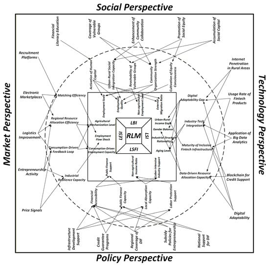
Figure 1. Multi-perspective impact framework of the RLM.

From a market perspective, DIF reduces transaction costs, improves search and matching, strengthens logistics and clarifies price signals. Recruitment platforms and electronic marketplaces shorten matching time and improve allocation, while better logistics and price discovery support entrepreneurship and local demand [29]. These channels most strongly reinforce the Labor Economic Sustainability Index LESI through more stable employment flows, higher productive capacity and stronger demand that sustains jobs over time [31,38]. Evidence shows that digital inclusive finance raises agricultural economic resilience and supports modernization through risk management and equipment investment, consistent with persistent gains measured by LESI [11,42].

From a policy perspective, public action expands the reach and reliability of digital finance through infrastructure provision, credit guarantees, regional coverage programs and support for entrepreneurship. These instruments widen access to formal finance for households and small firms, raise fiscal capacity for enforcement and safety nets, and improve wage settlement and job absorption [25,26]. The resulting protection and equitable access most strongly strengthen the Labor Security and Fairness Index LSFI, while also enabling inclusive growth in rural areas [8,9]. Empirical findings link digital inclusive finance to better factor allocation and higher resilience, which supports fairer labor outcomes in line with LSFI [11,12]. Financial inclusion is associated with lower poverty and narrower inequality, further grounding the fairness focus of LSFI [23,24,28].

From a technology perspective, innovation enables lasting inclusion through internet penetration in rural areas, use of fintech products, data driven credit assessment, secure transaction records and digital adaptability. Digital networks and platforms reduce information frictions and distance barriers, facilitate reallocation toward higher productivity activities and support industrial upgrading [38,43]. These effects most strongly improve the Labor Structure Index LSI by altering the sectoral mix and the distribution across groups, and by deepening market integration and employment growth when factor flows are enabled by digital finance [17,44]. Research highlights technology adoption and labor-saving modernization in farming, while cautioning that uneven diffusion can widen divides if not managed with inclusion in mind [31,39].

From a social perspective, inclusion, capability and trust determine the depth and quality of adoption. Financial literacy, coverage of vulnerable groups, community collaboration, equity norms and social capital accumulation increase effective participation and job search, raise local job quality and reduce excessive out migration [37]. These improvements most strongly lift the Labor Behavior Index LBI by moving participation, mobility and search intensity on both extensive and intensive margins [33,34]. Mobile money and e commerce expand networks and information and improve household welfare and employment capacity in rural settings, reinforcing the behavioral gains captured by LBI [6,45].

In summary, DIF supports the development of the RLM through market, policy, technology, and social channels. Grounded in these perspectives, we present a conceptual diagram (Figure 1) that organizes the pathways and guides the empirical design. To estimate these channels in a form that is both flexible and transparent, we combine econometric discipline with explainable machine learning. Conventional linear specifications struggle with nonlinearity, interactions, and multicollinearity, whereas purely machine learning approaches often provide limited attribution and are difficult to audit for policy use. We therefore obtain auditable indicator weights with AHM and FCE, and then fit a Random Forest with Gini importance and out of bag validation, tuned with PSO and GA, to capture nonlinear relations and county-level heterogeneity while preserving interpretable contributions. This integrated strategy allows us to test theory-consistent pathways and to report which channels matter, where they matter, and by how much.

3. Methodology

To rigorously investigate the impact of digital inclusive finance on the rural labor market, the research constructs a unified methodological framework that combines AHM-FCE weighting with the PSO-GA-RF model. By coupling Gini-based purity with OOB-driven generalization, the approach ensures both explanatory depth and robust predictive accuracy, as illustrated in Figure 2.

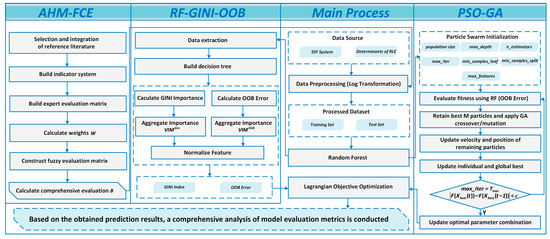
Figure 2. The methodology framework.

3.1. The AHM-FCE Method

The left-hand AHM–FCE panel of Figure 2 summarizes the construction of the rural labor market (RLM) index, which transforms raw county-level indicators into composite scores for the behavior, structure, security and fairness, and sustainability dimensions.

3.1.1. AHM Method

The Attribute Hierarchy Model (AHM) is an improved version of the Analytic Hierarchy Process (AHP) [46]. It has gained attention for its simplicity and the elimination of complex steps such as eigenvector calculations and consistency checks. In this research, we use the AHM method to evaluate the weights of RLM indicators. Compared with traditional AHP, AHM offers clear advantages in computational efficiency and practical application. It is especially suitable for decision-making scenarios that require quick evaluation. The specific steps are as follows:

STEP1: Construct a judgment matrix. We build the judgment matrix $A={\left(a_{ij}\right)}_{n\times n}$ by comparing the relative importance of each indicator pair. The matrix uses a nine-point scale with integer values from 1 to 9 to reflect different degrees of importance. When forming the matrix, ensure that each diagonal element satisfies $a_{ii}=1$. Then, to maintain symmetry, apply the following conditions:

$$\left\{\begin{array}{l}{a}_{\mathrm{ij}}>0\\ a_{ii}=1\\ a_{ji}=1/a_{ij}\end{array}\right.$$

(1)

where $1\le i\le n, 1\le j\le n,i\ne j$.

STEP2: Calculate the attribute judgment matrix. Use the following formula to transform the judgment matrix $A={\left(a_{ij}\right)}_{n\times n}$ into the attribute judgment matrix $B={\left({\mathrm{b}}_{ij}\right)}_{n\times n}$:

$$b_{ij}=\left\{ \begin{array}{ll}{\displaystyle \frac{\beta \kappa }{\beta \kappa +1}},\hfill & a_{ij}=\kappa \hfill \\ 0.5,\hfill & a_{ij}=1, i\ne j\hfill \\ 0,\hfill & i=j\hfill \\ {\displaystyle \frac{1}{\beta \kappa +1}},\hfill & a_{ij}=1/\kappa \hfill \end{array}\right.$$

(2)

where $\kappa$ is an integer greater than 1, and $\beta$ is usually set to 1 or 2. These parameters help adjust the spread and symmetry of the weight distribution.

STEP3: Determine the subjective weight. Use the following formula to calculate the relative attribute weights $W$ for each indicator $w$:

$$w={\displaystyle \frac{2}{n(n-1)}}{\displaystyle \sum _{i=1}^n{b}_{ij}}$$

(3)

where $n$ is the total number of evaluated indicators.

By applying the AHM method, we obtain the weight vector $W=\{w_1,w_2,\dots ,w_n\}$. These weights reflect each indicator’s relative importance in the overall evaluation and determine how strongly each observable labor indicator contributes to the composite RLM pillars in Figure 2 (for example, a larger weight on non-agricultural employment emphasizes structural adjustment in local labor dynamics).

3.1.2. FCE Method

Since the indicator weights in the Peking University Digital Financial Inclusion Index of China are based on expert judgment, and therefore involve some degree of subjectivity and fuzziness. The FCE method, grounded in fuzzy mathematics theory [47], effectively addresses these uncertainties by using membership functions to quantify subjective assessments. It also provides a multidimensional, multifactor analytical framework [48,49]. Therefore, the research applies the FCE method to measure the RLM index. The steps are as follows:

STEP1: Develop the multilevel evaluation index system. The first step is to identify the key factors affecting the RLM and then construct an evaluation index set based on Peking University’s digital inclusive finance indicators. A complete index framework is essential for assessing how digital inclusive finance influences rural labor market development. This system consists of three levels: goal, criteria, and indicators. Suppose the RLM evaluation index system is defined as $\mathcal{X}$, where each element in $\mathcal{X}$ represents a factor influencing rural labor development:

$$\mathcal{X}=\{X_1,X_2,\dots ,X_n\}$$

(4)

$$X_r=\{X_{r1},X_{r2},\dots ,X_{r{m}_r}\}$$

(5)

where $\mathcal{X}$ denotes the RLM evaluation index system; $X_1,\dots ,X_n$ are the key dimensions (criteria); for each dimension $X_r$, its indicator set is $X_r=\{x_{i1},\dots ,x_{r{m}_r}\}$. Here $n$ is the number of dimensions (four in the research), and $m_r$ is the number of indicators under $X_r$.

STEP2: Determine the evaluation criteria and ranks. This step establishes an evaluation set for all possible outcomes of the object being assessed. Suppose there are $k$ evaluation grades; define:

$$V=\{v_1,v_2,\dots ,v_k\}$$

(6)

where $v_j(j=1,\dots ,k)$ denotes an evaluation grade. Here $k$ is the number of grades, distinct from the number of factors $n$.

STEP3: The index weights are obtained from the AHM procedure in Section 3.1.1. Let $W=\{w_1,w_2,\dots ,w_n\}$ denote the weight vector of the $n$ indicators (with ${\sum }_{i=1}^n{w}_i=1$). These weights will be used in the fuzzy comprehensive evaluation.

STEP4: Determine the fuzzy assessment matrix. The fuzzy assessment matrix is vital in the AHM-FCE method because it captures the relationship between each indicator and the evaluation ranks. Suppose the membership of dimension $X_{\mathrm{i}}$ to evaluation grade $v_j$ is $r_{ij}$. The membership matrix has the form:

$$R=\left[\begin{array}{cccc}{r}_{11}& r_{12}& \dots & r_{1k}\\ r_{21}& r_{22}& \dots & r_{2k}\\ ⋮& ⋮& \ddots & ⋮\\ r_{n1}& r_{n2}& \dots & r_{nk}\end{array}\right]$$

(7)

where $R\in {\mathbb{R}}^{n\times k}$. Row $i$ corresponds to indicator $X_i$. Column $j$ corresponds to grade $v_j(j=1,\dots ,k)$. For each $i$, ${\sum }_{j=1}^k{r}_{ij}=1$ and $r_{ij}\in \left[\mathrm{0,1}\right]$. This matrix provides the main input for the final fuzzy comprehensive evaluation.

STEP5: Calculate a comprehensive evaluation score. Once the weight vector $W$ and the fuzzy assessment matrix $R$ are determined, we can compute the final evaluation result. The comprehensive evaluation vector $E$ is calculated using:

$$E=W\cdot R$$

(8)

To convert the aggregated memberships into a single crisp score, we apply a defuzzification vector:

$$F=E\cdot {\eta }^T$$

(9)

where $\mathbf{W}=(w_1,\dots ,w_n)\in {\mathbb{R}}^{1\times n}$ is the weight vector (${\sum }_{i=1}^n{w}_i=1$); $R=\left[r_{ij}\right]\in {\mathbb{R}}^{n\times k}$ is the membership matrix with $r_{ij}\in \left[\mathrm{0,1}\right]$ and ${\sum }_{j=1}^k{r}_{ij}=1$; $\mathbf{E}=(e_1,\dots ,e_k)\in {\mathbb{R}}^{1\times k}$; and $\mathsf{\eta }=({\eta }_1,\dots ,{\eta }_k)\in {\mathbb{R}}^{1\times k}$ assigns numerical scores to grades (e.g., $\mathsf{\eta }=\left(\mathrm{0.25,0.50,0.75,1.00}\right)$).

3.2. The PSO-GA-RF Method

The right-hand PSO–GA panel of Figure 2 summarizes the optimization and model-fitting procedure. PSO and GA are combined to search over random forest hyperparameters and feature subsets under the GINI–OOB objective, and the resulting model is then used in the “Main Process” panel to link digital inclusive finance to the RLM indices.

3.2.1. PSO Method

Particle Swarm Optimization (PSO) is a swarm-intelligence-based stochastic optimization algorithm proposed by Kennedy and Eberhart [50]. It simulates the cooperative behavior of individual agents in search of food. Compared with genetic algorithms (GA) or gravitational search algorithms (GSA), PSO dynamically updates personal best and global best solutions to balance global exploration and local exploitation. This approach avoids GA’s complex crossover and mutation operations, and it converges quickly with relatively low computational cost—making it suitable for high-dimensional, nonlinear problems.

In the research, PSO is used to optimize the key hyperparameters of the Gini–OOB index, allowing a more precise assessment of how digital inclusive finance affects the RLM. By adaptively tuning these hyperparameters, PSO improves the Gini–OOB index’s stability and predictive capability.

STEP1: Initialize the particle swarm. Set the population size $N$ and the search dimension $d$. Each particle is defined in Equation (10):

$$x_p=(x_{p1},x_{p2},\dots ,x_{pd}), v_p=(v_{p1},v_{p2},\dots ,v_{pd})$$

(10)

where $\mathrm{p}=1,\dots ,\mathrm{N}$ indexes particles and $\mathrm{q}=1,\dots ,\mathrm{d}$ indexes coordinates (hyperparameters or feature-mask entries). Positions are initialized as ${\mathrm{x}}_{\mathrm{p}\mathrm{q}}\sim \mathrm{U}({\mathcal{l}}_{\mathrm{q}},{\mathrm{u}}_{\mathrm{q}})$ and velocities as ${\mathrm{v}}_{\mathrm{p}\mathrm{q}}=0$. The search space is $[{\mathcal{l}}_1,{\mathrm{u}}_1]\times \cdots \times [{\mathcal{l}}_{\mathrm{d}},{\mathrm{u}}_{\mathrm{d}}]$. Integer hyperparameters are rounded at evaluation; categorical or Boolean choices are obtained by thresholding or encoding; continuous coordinates are used directly. Positions that exceed the bounds are clipped component-wise by $\mathrm{c}\mathrm{l}\mathrm{i}\mathrm{p}({\mathrm{x}}_{\mathrm{p}\mathrm{q}},{\mathcal{l}}_{\mathrm{q}},{\mathrm{u}}_{\mathrm{q}})$.

STEP2: Evaluate the fitness function. Let $\lambda \ge 0$ denote the sparsity coefficient that penalizes the proportion of selected features. For a candidate particle with decoded hyperparameters, the model is evaluated by $K$-fold cross-validation. In each fold, the random forest is trained on the training split and predictions are obtained for the validation split. The fitness is:

$$\mathit{Fitness}(x_i)={\displaystyle \frac{1}{K}}{\displaystyle \sum _{k=1}^K\frac{1}{n_k}}{\displaystyle \sum _{j\in {\mathcal{V}}_k}{(y_j-{\widehat{y}}_j)}^2}+\lambda {\displaystyle \frac{\left|S_{sel}\right|}{P}}$$

(11)

where $K=5$ unless stated otherwise. ${\mathcal{V}}_k$ is the validation index set in fold $k$ and $n_k=\left|{\mathcal{V}}_k\right|$. The inner index $j$ runs over validation instances in ${\mathcal{V}}_k$. $S_{\mathrm{s}\mathrm{e}\mathrm{l}}$ is the selected feature set and $P$ is the total number of candidate features. Let $\mathcal{E}={\bigcup }_{k=1}^K{\mathcal{V}}_k$ denote the evaluation set formed by pooling validation folds. Out-of-bag $R^2$ is defined in Equation (12):

$$R_{\mathit{OOB}}^2=1-{\displaystyle \frac{{\displaystyle \sum _j(}{y}_j-{\widehat{y}}_j^{\mathrm{OOB}}{)}^2}{{\displaystyle \sum _j(}{y}_j-\overline{y}{)}^2}}$$

(12)

STEP3: Update personal best and global best. Since the objective is to minimize $\mathrm{F}\mathrm{i}\mathrm{t}\mathrm{n}\mathrm{e}\mathrm{s}\mathrm{s}$ in (11), the personal best and global best are updated as follows:

$$p_b(t)=\arg \underset{\tau \le t}{\min }\mathrm{Fitness}(x_p(\tau ))$$

(13)

$$p_g(t)=\arg \underset{p\in S(t)}{\min }\mathrm{Fitness}(x_p(t))$$

(14)

where $p_b\left(t\right)$ is the index of particle $p$’s best historical configuration up to iteration $t$; $p_g(t)$ is the index of the best configuration in the swarm at iteration $t$; and $S(t)$ denotes the set of active particles (typically $S\left(t\right)=\{1,\dots ,N\}$).

STEP4: Update velocity and position. A particle’s search direction and step size are determined by its velocity. The update equations are:

$$v_{pq}(t+1)=\omega (t)v_{pq}(t)+c_1{r}_{1p}(x_{pq}^b(t)-x_{pq}(t))+c_2{r}_{2p}(x_q^g(t)-x_{pq}(t))$$

(15)

$$x_p(t+1)=x_p(t)+v_p(t+1)$$

(16)

where $p=1,\dots ,N$ and $q=1,\dots ,d$; $r_{1p},r_{2p}\sim U\left(\mathrm{0,1}\right)$ are resampled at each iteration; $c_1,c_2>0$ are acceleration coefficients (commonly $c_1=c_2=2$); $x_{pq}^{ b}\left(t\right)$ is the $q$-th coordinate of particle $p$’s personal best, and $x_q^{ g}\left(t\right)$ is the $q$-th coordinate of the global best. The inertia weight $\omega \left(t\right)$ balances exploration and exploitation and follows:

$$\omega (t)=({\omega }_{\max }-{\omega }_{\min })e^{-500{(t/T)}^2}+{\omega }_{\min }$$

(17)

where ${\omega }_{\mathrm{m}\mathrm{a}\mathrm{x}}$ and ${\omega }_{\mathrm{m}\mathrm{i}\mathrm{n}}$ are the initial and terminal inertia weights, $T$ is the maximum number of iterations, and $t$ is the current iteration. To keep all hyperparameters within valid ranges, the updated position is clipped component-wise:

$$x_{pq}(t+1)=\mathrm{clip}(x_{pq}(t+1),{\mathcal{l}}_q,u_q)$$

(18)

STEP 5: Termination criteria. PSO runs iteratively and stops when any of the following conditions is met:

$$\left|\mathrm{Fitness}(x_{p_g}(t))-\mathrm{Fitness}(x_{p_g}(t-1))\right|<\epsilon \mathit{or} t=T_{max}$$

(19)

where $\epsilon >0$ is a tolerance threshold and $T_{\mathrm{m}\mathrm{a}\mathrm{x}}$ is the preset iteration limit.

3.2.2. GA Method

Genetic Algorithms (GA) simulate natural selection and genetic principles through selection, crossover, and mutation [51]. Compared with Particle Swarm Optimization (PSO), GA maintains population diversity during global search and avoids local optima. In the research, GA optimizes the hyperparameters and feature selection of a Random Forest (RF) model to enhance predictive performance and robustness.

STEP1: Initialize the Population. During initialization, randomly generate $N$ individuals in the search space. Each individual is written as shown in Equation (20):

$$x_p=(x_{p1},x_{p2},\dots ,x_{pm}),p=1,2,\dots ,N$$

(20)

where $m$ is the search dimension. Each gene $x_{pq}(q=1,\dots ,m)$ lies within bounds $[{\mathcal{l}}_q,u_q]$; integer genes are rounded at evaluation, categorical or Boolean genes are obtained by encoding or thresholding, and continuous genes are used directly. When a feature mask is used, the selected set is $S_{\mathrm{s}\mathrm{e}\mathrm{l}}=\{q: x_{pq}=1\}$.

STEP2: Evaluate the fitness function. The fitness used by GA is the same as in Equation (11), and the algorithm minimizes this fitness.

STEP3: To match the minimization objective, we define the selection score as:

$$F(x_p)={\displaystyle \frac{1}{\epsilon +\mathit{Fitness}(x_p)}}$$

(21)

where $\epsilon >0$ is a small constant for numerical stability. Using roulette-wheel (fitness-proportional) selection, the probability of choosing parent $X_p$ is:

$$P(x_p)={\displaystyle \frac{F(x_p)}{{\displaystyle \sum _{r=1}^{N}F}(x_{p\prime })}}$$

(22)

where p′ is a dummy individual index running from $1$ to $N$.

STEP4: Crossover and Mutation. Let the selected parents be $\{{\mathbf{x}}^{\left(s\right)}{\}}_{s=1}^L\subset {\mathbb{R}}^m$, where $L\ge 2$ denotes the number of parents and the superscript $\left(s\right)$ is a parent label (not an exponent or time index). For each gene $q=1,\dots ,m$, define a one-hot mask $\{c_{s,q}{\}}_{s=1}^L\subset \{\mathrm{0,1}\}$ satisfying ${\sum }_{s=1}^L{c}_{s,q}=1$. The child is defined component-wise by:

$$x_q^{(new)}={\displaystyle \sum _{s=1}^L{c}_{s,q}}{x}_q^{(s)}, q=1,\dots ,m$$

(23)

After crossover, each gene mutates independently with probability $p_m\in \left(\mathrm{0,0.5}\right]$:

$$x_q(t+1)=\left\{\begin{array}{ll}{x}_q(t)+\delta \hfill & \mathit{with} \mathit{probability} {\displaystyle \frac{p_m}{2}}\hfill \\ x_q(t)-\delta \hfill & \mathit{with} \mathit{probability} {\displaystyle \frac{p_m}{2}}\hfill \\ x_q(t)\hfill & \mathit{with} \mathit{probability} 1-p_m\hfill \end{array}\right.$$

(24)

where $p_m\in \left(\mathrm{0,0.5}\right]$ is the per-gene mutation rate and $\delta >0$ is the mutation magnitude. The mutated coordinate $x_q(t+1)$ replaces $x_q\left(t\right)$ and, if it lies outside the bounds, it is projected onto the interval $[{\mathcal{l}}_q,u_q]$ (component-wise). All mutations are applied independently across genes.

STEP5: Termination Criteria.

$$\left|\mathrm{Fitness}(x^g(t))-\mathrm{Fitness}(x^g(t-1))\right|<\epsilon \mathrm{or} t=T_{max}$$

(25)

3.2.3. RF Method

Random Forest (RF) is an ensemble learning algorithm proposed by Breiman. It is known for its robustness and strong generalization ability. Due to its performance in high-dimensional and nonlinear data, RF has become a powerful tool for analyzing complex data in fields such as financial time series, credit scoring, and rural economic indicator forecasting. The main steps of the RF model are as follows (see also the RF–GINI–OOB block in Figure 2):

STEP1: Data Sampling. RF uses Bootstrap Sampling to extract $N$ subsets from the training dataset $D=\{(x_i,y_i)|i=1,2,\dots ,N\}$. Each subset is the same size as the original dataset and is sampled with replacement. The sampled dataset for the k-th tree is denoted as:

$$D_k\prime =\{(x_i,y_i)|i\in S_k\}$$

(26)

where k trees are trained. $S_k$ represents the index set of sampled data for the k-th tree. This preserves data diversity and helps the model capture complex patterns in financial data.

STEP2: Decision Tree Building. For each sampled dataset $D_k\prime$, a decision tree is constructed. RF randomly selects a feature subset $F_k$ from the full feature set $F$. The selection process is defined as:

$$F_k=\left\{f_1,f_2,\dots ,f_m\right\}\subseteq F,\hspace{1em}\left|F_k\right|=m,\hspace{1em}1\le \mathrm{m}\le \left|F\right|$$

(27)

The tree $T_k$ is then built using both $D_k\prime$ and the feature subset $F_k$. The tree is optimized by minimizing the following objective function:

$$T_k=arg\underset{T}{\min }{\displaystyle \sum _{(x_i,y_i)\in D_k^{\prime }}L(y_i,T(x_i;F_k))}$$

(28)

where $F_k$ is the selected feature subset. $T_k$ is the decision tree trained on $D_k\prime$ and $F_k$. $L$ is the loss function used for optimization. Random feature selection reduces correlation among trees. This improves model performance and enhances generalization [52].

STEP3: Ensemble Prediction. A total of $N_d$ decision trees $T_1,T_2,\dots ,T_{N_d}$ are combined to form the RF model. The final prediction is obtained by aggregating the outputs of all trees.

For regression tasks, the output is calculated by weighted averaging:

$$\widehat{y}={\displaystyle \frac{1}{N_d}}{\displaystyle \sum _{k=1}^{N_d}{T}_k(x)}$$

(29)

For classification tasks, the output is determined by majority voting:

$$\widehat{y}=\arg \underset{c\in \mathcal{C}}{\max }{\displaystyle \sum _{k=1}^{N_d}\mathbb{I}(T_k(x)}=c)$$

(30)

where $\mathbb{I}$ is the indicator function. It equals 1 if $T_k(x)=c$, and 0 otherwise. $\mathcal{C}$ denotes the set of all classes.

The ensemble nature of random forests provides strong advantages in handling high-dimensional and heterogeneous data. Figure 3 illustrates the process of bootstrap sampling, feature selection, decision tree construction, and final ensemble prediction.

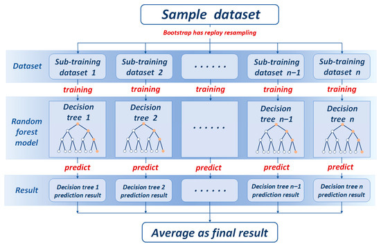
Figure 3. Schematic diagram of the random forest algorithm.

3.2.4. The PSO-GA-RF Fitting Method

The research proposes an improved hybrid optimization algorithm: PSO-GA. It is used to optimize the hyperparameters and feature selection of the Random Forest (RF) model. The goal is to improve prediction accuracy and stability of the model based on the Gini–OOB index when measuring the impact of digital inclusive finance on the rural labor market. The algorithm integrates the advantages of two swarm intelligence methods: PSO and GA. PSO performs dynamic updates based on individual best ($P_{b_i}(t)$) and global best ($P_g(t)$) positions (see Equations (13) and (14)), enabling fast convergence to the local optimum. GA applies selection, crossover, and mutation (see Equations (21)–(24)) to broaden the search space and avoid premature convergence.

Specifically, the algorithm begins by randomly initializing a population within the predefined search space. The update process follows the PSO rules (see Equations (10)–(19)). After several iterations, the top M particles with the lowest fitness values are retained. These M particles serve as the initial population for the GA phase. At this stage, parent selection probabilities are computed using Equation (22). The population undergoes roulette wheel or tournament selection. Single-point crossover is then applied to generate new individuals (refer to Equation (23)). Mutation is performed according to Equation (24), where each gene has a probability $p_m$ of being perturbed. This enhances population diversity.

After GA optimization, the newly generated particles are merged with those not selected for GA. The combined population enters the next PSO iteration. This alternating process continues until the convergence condition defined in Equation (19) is satisfied. The final output is the optimized set of RF model hyperparameters and selected feature subset.

As illustrated in Figure 4, and summarized in the PSO–GA panel of Figure 2, this hybrid search explores a mixed continuous–discrete space of RF hyperparameters and feature masks under a non-convex GINI–OOB objective. Compared with grid search, it avoids the curse of dimensionality on a fixed grid and can adaptively concentrate evaluations in promising regions. Unlike Bayesian optimization, it does not require specifying a smooth surrogate response surface, which is advantageous in our noisy, high-dimensional county–year setting. This makes PSO–GA particularly suitable for capturing nonlinear DIF–RLM relations while maintaining computational tractability.

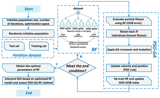
Figure 4. The PSO-GA-RF algorithm flowchart.

3.3. Construction of the GINI–OOB Coefficient

3.3.1. GINI Index Method

In the field of machine learning, the GINI Index is widely used in decision tree algorithms, especially in classification and regression trees (CART). The GINI Index is a metric for evaluating the purity of a dataset. It measures how samples are distributed across different classes and quantifies the inequality among them. During the construction of decision trees, the GINI Index evaluates the splitting capability of each feature. Features with lower GINI Index values are selected to improve node purity. In addition, the GINI Index guides tree growth by indicating when a node should be split or terminated. This enhances the efficiency and accuracy of decision trees in data processing, making them suitable for predictive modeling tasks. For financial data, optimized decision tree structures help capture complex variable relationships and improve model performance in financial risk assessment and user behavior prediction [53].

To measure feature importance, we adopt VIM to quantify the contribution of each feature to model prediction. Based on the GINI Index, let there be $p$ features $M_1,M_2,M_3,\dots ,M_p$, with $K$ decision trees and $A$ classes. We now calculate the GINI Index score for each feature $M_p$ using the $VI{M}_p^{(Gini)}$. The specific calculation is as follows:

STEP1: GINI Calculation. The GINI Index is defined as ${\mathit{GI}}_y^{(k)}$ and calculated by:

$$G{I}_N^k={\displaystyle \sum _{a=1}^{\left|A\right|}{\displaystyle \sum _{a\prime \ne a}{x}_{na}^k}}{x}_{na\prime }^k=1-{\displaystyle \sum _{a=1}^{\left|A\right|}{\left(x_{na}^k\right)}^2},\hspace{1em}x\in R$$

(31)

In Equation (31), $\left|A\right|$ denotes the number of categories. $x_{na}$ is the proportion of class $a$ at node $n$.

STEP2: GINI-Based Importance. The importance of feature $M_p$ at node $n$ in the k-th decision tree is measured by the change in GINI Index after the node splits. It is computed as:

$$VI{M}_p^{(Gini)(k)(n)}=G{I}_n^k-G{I}_I^k-G{I}_O^k$$

(32)

where ${\mathit{GI}}_I^{(k)}$ and ${\mathit{GI}}_O^{(k)}$ represent the GINI Index of the two child nodes after the split, as defined in Equation (31).

STEP3: Feature Importance Aggregation. The importance of feature $M_p$ in tree k is the sum of its importance over all relevant nodes in set $\mathcal{Y}$:

$$VI{M}_p^{(Gini)(k)}={\displaystyle \sum _{n\in \mathcal{Y}}VI{M}_p^{(Gini)(k)(n)}}$$

(33)

The total importance of feature $M_p$ across all K trees is:

$$VI{M}_p^{Gini}={\displaystyle \sum _{k=1}^{K}VI{M}_p^{(Gini)(k)}}$$

(34)

STEP4: Feature Normalization. To compare the importance across all features, normalize the values as follows:

$$VI{M}_{p_0}^{Gini}={\displaystyle \frac{VI{M}_p^{Gini}}{{\displaystyle {\sum }_{p\prime =1}^{p}VI{M}_{p\prime }^{Gini}}}}$$

(35)

3.3.2. OOB Index Method

In the Random Forest (RF) model, multiple decision trees are built using bootstrap sampling. Each bootstrap sample is generated with replacement from the training data. As a result, some training samples are not used by certain trees. These unused samples form the Out-of-Bag (OOB) dataset. The OOB Index provides a natural validation set during training. It is used to assess the model’s generalization ability. This is especially valuable in complex settings such as digital inclusive finance and rural labor economies. In these contexts, the OOB Index helps the model handle high-dimensional and structured data, improving both robustness and adaptability.

The OOB Index is not only useful for model performance evaluation. It also supports feature importance analysis. In feature importance estimation, the replacement of feature $M_p$ is used to assess its relative contribution to model prediction accuracy. Specifically, the baseline OOB error is first computed using the original (unshuffled) data. Then, feature $M_p$ is permuted, and a new OOB error is calculated. The difference between these two errors reflects the importance of $M_p$ [54]. The main steps of this method are described below.

STEP1: OOB Error Calculation. The importance of feature $M_p$ is measured by the change in OOB error before and after permutation. This difference reflects the predictive contribution of $M_p$ to financial data. It captures effects from variables such as credit risk, income level, and core economic indicators. The permutation process is repeated across all decision trees. The average result is used to calculate the overall permutation importance of variable $M_{p_0}$ in the random forest, denoted as $VI{M}_{p_0}^{OOB}$, as defined in Equation (36):

$$VI{M}_{p_0}^{OOB}={\displaystyle \frac{{\displaystyle \sum _{s=1}^{{\xi }_s^{\prime }}}O(T_s=T_s^k)}{{\xi }^k}}-{\displaystyle \frac{{\displaystyle \sum _{s=1}^{{\xi }_s^{\prime }}}O(T_s=T_{s,{\pi }_y}^k)}{{\xi }^k}}$$

(36)

where ${\xi }^k$ is the number of samples in the OOB set for the k-th tree. ${\xi }_s^{\prime }$ denotes the subset of samples related to the OOB data, O(x) is an indicator function: it returns 1 if the input is true, otherwise 0. $T_s\in \{0,1\}$ is the true label of sample s. $T_s^k\in \{0,1\}$ is the prediction of tree k before permutation. $T_{s,{\pi }_y}^k\in \{0,1\}$ is the prediction after permuting feature $M_{p0}$. If a sample does not appear in the k-th tree, it is excluded. If there is no difference, $VI{M}_j^{(OOB)}=0$.

STEP2: Aggregate Importance Across Trees. In a random forest, the overall permutation importance of the p-th feature, denoted as $VI{M}_p^{OOB}$, is defined by Equation (37):

$$VI{M}_p^{OOB}={\displaystyle \frac{{\displaystyle \sum _{p_0=1}^{K\prime }VI{M}_{p_0}^{(OOB)(k)}}}{K}}$$

(37)

where $K$ represents the total number of decision trees in the forest, and $K\prime$ denotes the number of trees that include the classification task.

3.3.3. The GINI–OOB Coefficient Coupling

To balance between the purity-driven importance and the model’s generalization ability, we propose a GINI–OOB hybrid weighting approach. This method combines the GINI Index $VI{M}_p^{GINI}$ and OOB-based permutation importance $VI{M}_p^{OOB}$, aiming to minimize redundancy while enhancing robustness. It is particularly suitable for complex, high-dimensional datasets commonly found in credit scoring, risk analysis, and multi-index prediction tasks.

STEP1: Define GINI–OOB Objective. We construct an optimization objective based on the GINI Index. This objective integrates the GINI Index and OOB permutation importance, and is defined as follows:

$$\left\{\begin{array}{ll}\min F=& {\displaystyle \sum _{p=1}^K(W_p\cdot }ln{\displaystyle \frac{W_p}{VI{M}_p^{Gini}}}) +{\displaystyle \sum _{p=1}^K(W_p}\cdot ln{\displaystyle \frac{W_p}{VI{M}_p^{OOB}}})\\ s.t.& {\displaystyle \sum _{p=1}^K{W}_p}=1 ,W_p\ge 0\end{array}\right.$$

(38)

STEP2: Derive Feature Weights. The above optimization problem is solved using the Lagrange multiplier method. The Lagrangian function is formulated as:

$$L={\displaystyle \sum _{p=1}^K(W_p\cdot ln\frac{W_p}{VI{M}_p^{Gini}})}+{\displaystyle \sum _{p=1}^K(W_p\cdot ln\frac{W_p}{VI{M}_p^{OOB}})}+\lambda (1-{\displaystyle \sum _{p=1}^K{W}_p})$$

(39)

STEP3: Aggregated Feature Weights. Combining the GINI Index and OOB importance, we obtain the final feature weights. These weights reflect a balanced contribution of both purity and generalization:

$$W_p={\displaystyle \frac{\sqrt{VI{M}_p^{Gini}\cdot VI{M}_p^{OOB}}}{{\displaystyle \sum _{p=1}^K\sqrt{VI{M}_p^{Gini}\cdot VI{M}_p^{OOB}}}}}$$

(40)

3.4. Evaluation Metrics

The research adopts three regression evaluation metrics: Mean Squared Error (MSE), Coefficient of Determination ($R^2$), and Mean Absolute Percentage Error (MAPE). These metrics quantitatively assess model prediction accuracy and enable performance comparisons [55]:

$$MSE={\displaystyle \frac{1}{N}}{\displaystyle \sum _{i=1}^N{(Y_i-Z_i)}^2}$$

(41)

$$R^2=1-{\displaystyle \frac{{\displaystyle \sum _{i=1}^N{(Y_i-Z_i)}^2}}{{\displaystyle \sum _{i=1}^N{(Y_i-\overline{Y})}^2}}}$$

(42)

$$MAPE={\displaystyle \frac{1}{N}}{\displaystyle \sum _{i=1}^N\left|\frac{Y_i-Z_i}{Y_i}\right|}\times 100\%$$

(43)

In the above formulas, $Y_i$ represents the actual observed value and $Z_i$ denotes the predicted value. MSE measures the average squared deviation between predictions and actual values. Lower MSE indicates better predictive accuracy and robustness. $R^2$ quantifies the explanatory power of the model for rural labor economic fluctuations. A value closer to 1 indicates stronger explanatory capability. MAPE captures the average relative percentage error between predicted and actual values, providing an intuitive interpretation of prediction accuracy.

In the empirical analysis, these metrics are computed under a five-fold cross-validation scheme on the county–year panel, and the reported values are averaged over the validation folds. During training, out-of-bag (OOB) error is simultaneously monitored through the GINI–OOB objective in Section 3.3. Consistent MSE, RMSE, MAE, MAPE, SMAPE and $R^2$ values across folds, counties and years, together with stable OOB errors, indicate that the PSO–GA–RF specification generalizes well rather than overfitting a narrow subset of observations. Data are split once into 80% training and 20% testing by county; all model selection uses five-fold cross-validation on the training set, and final metrics are computed on the held-out test set with the same normalization parameters learned from the training data.

4. Results

4.1. Data Collection and Pre-Processing

Jiangsu Province, located in eastern coastal China (longitude 116°18′–121°57′, latitude 30°45′–35°20′), covers an area of approximately 100,000 square kilometers. As one of China’s leading economic powerhouses, Jiangsu accounted for 10.15% of the national GDP as of 2024. According to the 2022 Digital Jiangsu Development Report [56], the province’s digital economy exceeded 5.1 trillion RMB by the end of 2021, ranking second nationwide and contributing 11.8% to the national total [57]. Despite its strong economic performance, Jiangsu exhibits significant internal disparities. In particular, rural areas lag behind urban centers in terms of development. This pronounced regional imbalance presents an ideal setting for investigating the impact of digital inclusive finance on the RLM. The findings are expected to offer both generalizable insights and practical policy implications. The study uses panel data from 58 counties in Jiangsu Province for the period 2014–2023. The RLM Index is calculated using the Gini–OOB method. Indicator data are obtained from China County Statistical Yearbook [58], Jiangsu Statistical Yearbook [59], Jiangsu Rural Development Yearbook [60], Jiangsu Agricultural Statistics Yearbook [61], and the EPS Data Platform. Official local government reports and publicly available data sources are also consulted.

To ensure consistency across sources and years, indicator definitions were harmonized, overlapping series were cross-checked, and time trends were inspected for structural breaks; counties with missing or inconsistent values were corrected using local records or excluded after robustness checks. In summary, descriptive statistics are shown in Table 3. The mean and standard deviation values reveal substantial cross-county heterogeneity in several key indicators: employment scale X₁₁, wage level X₁₂, external migration X₁₄, social protection X₃₃ and mechanization X₄₁ all have wide interquartile ranges and large standard deviations relative to their means, indicating that a few counties concentrate high employment, earnings and capital intensity while many remain far below the provincial frontier. By contrast, education X₂₁, gender balance X₂₂, the non-agricultural employment share X₂₄ and the labor income ratio X₃₂ exhibit narrower ranges and smaller variances, suggesting more homogeneous basic demographic and income structures. The joint dispersion of X₄₁ and X₃₂ implies that counties achieving higher mechanization also tend to record above-average labor income ratios, a pattern that is reflected in the north–south gradient of the spatial maps presented later. Taken together, these descriptive features depict a behaviorally active but structurally uneven rural labor market and indicate substantial scope for digital inclusive finance to support lagging counties by easing credit constraints for mechanization, upgrading job quality and strengthening social protection.

Table 3. Data statistical characteristics.

	MIN	25%	50%	75%	MAX	MEAN	STD
X11 (10,000 persons)	0.51	22.36	35.72	43.01	82.32	34.35	14.39
X12 (CNY/Person)	4212	8669.75	11,999	16,079.58	24,741.66	12,701.84	4842.66
X13 (ratio)	0.45	0.64	0.76	0.83	0.93	0.74	0.12
X14 (ratio)	19.68	92.18	148.48	223.78	12,901.96	201.08	581.25
X21 (ratio)	1.31	1.82	1.94	2.04	2.29	1.92	0.17
X22 (ratio)	0.41	0.47	0.48	0.5	0.62	0.49	0.03
X23 (ratio)	0.2	0.4	0.49	0.62	1.59	0.52	0.18
X24 (ratio)	0.45	0.68	0.77	0.85	1.11	0.77	0.13
X31 (ratio)	1.4	7.46	10.17	12.88	27.71	10.18	4.29
X32 (ratio)	0.38	0.69	0.76	0.81	0.98	0.75	0.09
X33 (ratio)	0.15	4.99	8.66	18.49	41.1	12.12	9.46
X41 (kW)	2.48	34.12	59.58	93.99	233.15	69.5	44.54
X42 (ratio)	0.02	0.66	1.02	1.25	2.5	1	0.42
X43 (ratio)	0.08	0.13	0.16	0.18	0.48	0.16	0.05

To account for differences in units and magnitudes among the indicators in the digital financial index system, direct calculation of composite scores is not feasible. Therefore, the research first categorizes the evaluation indicators into two types based on their directional nature and applies the Max-Min Method for standardization. The calculation formulas are as follows:

$$x_{ij}^{\prime }={\displaystyle \frac{x_j-x_{\min }}{x_{\max }-x_{\min }}}$$

(44)

$$x_{ij}^{\prime }={\displaystyle \frac{x_{\max }-x_j}{x_{\max }-x_{\min }}}$$

(45)

where $x_{ij}^{\prime }$ denotes the normalized value of indicator j for observation i, and $x_j$ is the original value. Equation (44) is used for positively oriented indicators, while Equation (45) is applied to negatively oriented indicators.

To reduce the inclusion of lagged variables and prevent prediction failure caused by multicollinearity, the research uses the Pearson correlation coefficient to test for collinearity among RLM indicators. The significance level is set at 0.05. A correlation coefficient with an absolute value greater than 0.9 is considered to indicate a strong correlation. As shown in Figure 5, the Pearson correlation between X₁₄ (External Migration Ratio) and X₂₂ (Gender Balance) is 0.96, indicating a strong relationship. Therefore, X₂₂ is excluded to minimize the impact of multicollinearity on predictive performance.

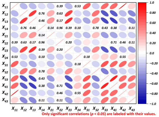
Figure 5. Correlation matrix of standardized data.

Beyond this screening role, Figure 5 also reveals several meaningful correlation clusters. External migration (X₁₄) and gender balance (X₂₂) form the core of the system: counties with higher migration and more skewed gender structures tend to be those with higher wages, higher labor-income shares and closer links to non-agricultural employment and mechanization, while low-migration, more balanced counties lie at the opposite end. A second, smaller cluster connects the non-agricultural employment share, land productivity and mechanization, suggesting that structural upgrading and capital deepening evolve jointly rather than in isolation. These bundled patterns imply that DIF is likely to affect rural labor outcomes through heterogeneous structural pathways, reinforcing upgrading and capital deepening in some counties while in others primarily easing migration-related and protection-related pressures.

4.2. RLM Measure

4.2.1. Calculation of AHM-FCE Weights

Although prior work links digital inclusive finance to rural macroeconomic outcomes, a dedicated and auditable evaluation system for its effects on the rural labor market remains underdeveloped. We therefore conducted a protocol-driven scoping review of peer-reviewed studies and policy documents to construct the indicator framework. To enhance face validity, two external domain experts (rural finance; labor policy) reviewed the draft taxonomy and channel linkages. Their comments were advisory and non-binding. The resulting evaluation matrix traces DIF’s channels to the RLM across three pillars—labor structure, equity & protection, and sustainability—and makes the inter-indicator relations explicit for econometric testing.

Weights were then estimated via the AHM–FCE pipeline. Pairwise relevance assessments formed the judgment matrix and, following Equation (1), the attribute discrimination matrix D. Fuzzy Comprehensive Evaluation (FCE) aggregated standardized indicators within and across pillars to obtain the final weights. The weight vector is summarized in Table 4, where for each indicator we report: W_{AHM_1} (its within-subdimension AHM weight), W_{AHM_2} (the AHM weight of its subdimension in the overall hierarchy), W_AHM (=W_{AHM_2} × W_{AHM_1}, the global AHM weight), W_FCE (the FCE score on standardized data), and W_AHM–FCE (=W_AHM × W_FCE, normalized). For illustration using Table 4’s numbers, X₁₁ has W_{AHM_2} = 0.38 (for subdimension X₁ in the overall RLM) and W_{AHM_1} = 0.11 (X₁₁ within X₁E_AHM ≈ 0.38 × 0.11 = 0.04; with W_FCE = 0.74, its W_AHM–FCE ≈ 0.04 × 0.74 = 0.03.

Table 4. Combined weights from AHM analysis.

	AHM			FCE	WAHM-FCE
	WAHM_1	WAHM_2	WAHM	WFCE
X11	0.38	0.11	0.04	0.74	0.03
X12		0.31	0.12	0.68	0.08
X13		0.58	0.22	0.60	0.13
X14		0.10	0.04	0.55	0.02
X21	0.20	0.75	0.15	0.69	0.10
X23		0.17	0.03	0.56	0.02
X24		0.08	0.02	0.50	0.01
X31	0.24	0.53	0.13	0.74	0.10
X32		0.30	0.07	0.68	0.05
X33		0.17	0.04	0.60	0.02
X41	0.18	0.54	0.10	0.74	0.07
X42		0.29	0.05	0.68	0.03
X43		0.17	0.03	0.60	0.02

As shown in Table 4, indicator X₁₃ (non-agricultural employment level) exhibits the highest comprehensive weight (0.220), highlighting its dominant influence on the labor behavior dimension. In contrast, indicator X₂₃ (Aging Level) holds the lowest weight (0.020), suggesting a relatively minor role in the labor economy evaluation system. At the dimensional level, labor behavior contributes most significantly (0.380), followed by employment quality (0.240), while labor sustainability has comparatively limited impact (0.180). The associated RLM density distribution is shown in Figure 6.

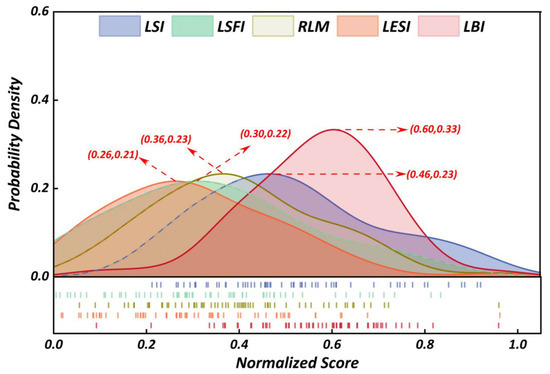
Figure 6. RLM score distribution.

Figure 6 presents kernel density estimates for the five normalized indices of the rural labor market (RLM, LBI, LSI, LSFI, and LESI). The LBI curve exhibits the highest peak and a comparatively high mean (≈0.60 on the [0, 1] scale), indicating broadly strong behavioral performance across counties. By contrast, LSI is concentrated at lower values (≈0.30), suggesting limited long-term development capacity for most units. Distributional shapes differ: LSFI, LESI, and the composite RLM are approximately symmetric and unimodal, whereas LBI is positively skewed and LSI negatively skewed, revealing asymmetric performance tails across dimensions.

Figure 7 shows clear and dimension specific geography. In LBI the strongest values cluster in the northwest. Sheyang SY and Shuyang SYG stand out, while many southern counties record low values. LSI displays an even sharper north–south gradient. Sheyang SY, Shuyang SYG and Baoying BY lead on structural upgrading. Counties around Jingkou JK and Runzhou RZ are much lower, which is consistent with smaller rural shares and slower movement into nonagricultural jobs.

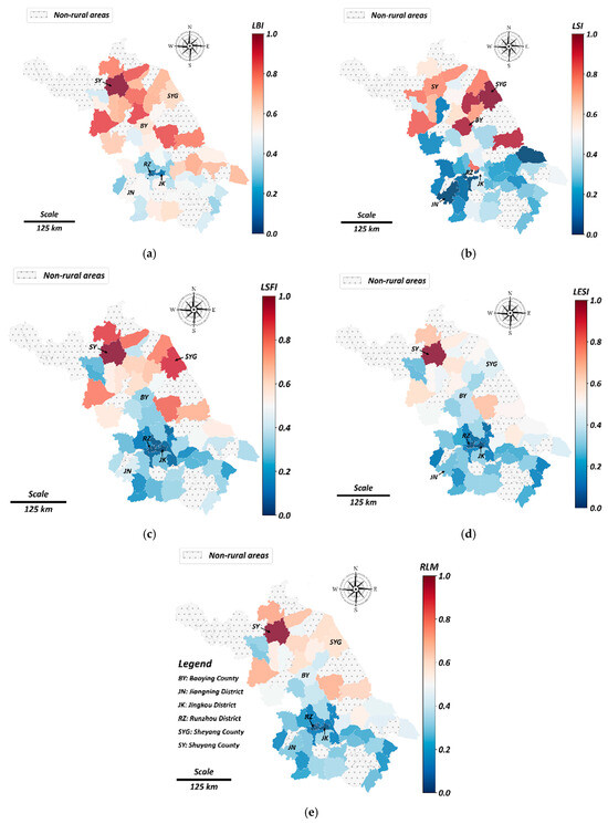
Figure 7. Spatial distribution of RLM indicator scores. (a) LBI, (b) LSI, (c) LSFI, (d) LESI (e) RLM.

LSFI broadly follows the same gradient, although the contrast is milder. This indicates wider improvements in security and fairness that extend beyond the leading group. In LESI the high values lie along a northern and central belt with Sheyang SY again prominent. Many southern counties remain in the lower terciles, which signals persistent gaps in equity and social protection.

The composite RLM map integrates these patterns. A high-value cluster forms in the northwest and low to mid values appear across the south and the southeast. Baoying BY forms a secondary node among otherwise moderate central scores. Several local exceptions are visible. Some areas around Runzhou RZ and Jingkou JK score higher on LESI than on LSI, which suggests that safety nets and transfers can partially offset structural weaknesses. Scores are averaged over 2014 to 2023 and scaled between zero and one. Hatched cells mark non rural areas. The overall configuration points to structured spatial disparities that merit further investigation.

Global spatial autocorrelation is strongly positive. Moran’s I equals 0.568 for RLM with permutation p = 0.001; the pillar indices are LBI 0.544 (p = 0.001), LSI 0.410 (p = 0.001), LSFI 0.560 (p = 0.001), and LESI 0.499 (p = 0.001), confirming pronounced clustering patterns across counties.

4.2.2. A Probe into the Factors Affecting RLM

To calculate the importance of each variable affecting the Rural Labor Market (RLM), all modeling and computational procedures were executed in the PyCharm 2023.2 environment using Python 3.11.

The hyperparameters of the Random Forest model were optimized using a hybrid PSO-GA algorithm with 50 particles and 50 iterations, incorporating a GA operation every 5 generations. The parameter search space included: number of trees (50–200), maximum depth (3–30), minimum samples for split (2–20), minimum samples per leaf (1–20), and max features (0.1–1.0). A five-fold cross-validation was employed to ensure model robustness. The fitness function was defined as a composite value combining MSE and MAPE with a regularization factor λ = 1000. The model was trained on data from 2014 to 2023 using normalized explanatory variables, and evaluated using six metrics: MSE, RMSE, MAE, MAPE, SMAPE, and R². Feature importance was assessed through both Gini index and OOB error, and the final importance scores were obtained by applying a Lagrangian coupling strategy to synthesize the two. The temporal dynamics of importance scores and optimization results are illustrated in Figure 8. For completeness, the detailed yearly hyperparameter settings, feature-importance rankings, and model-comparison metrics are reported in Appendix A (Table A1, Table A2, Table A3 and Table A4 and Figure A1).

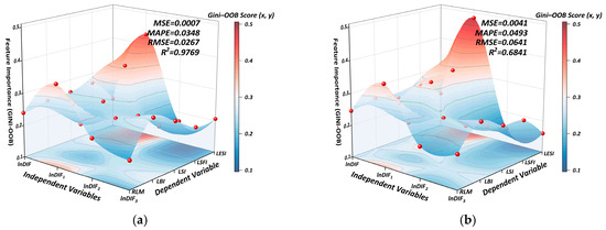
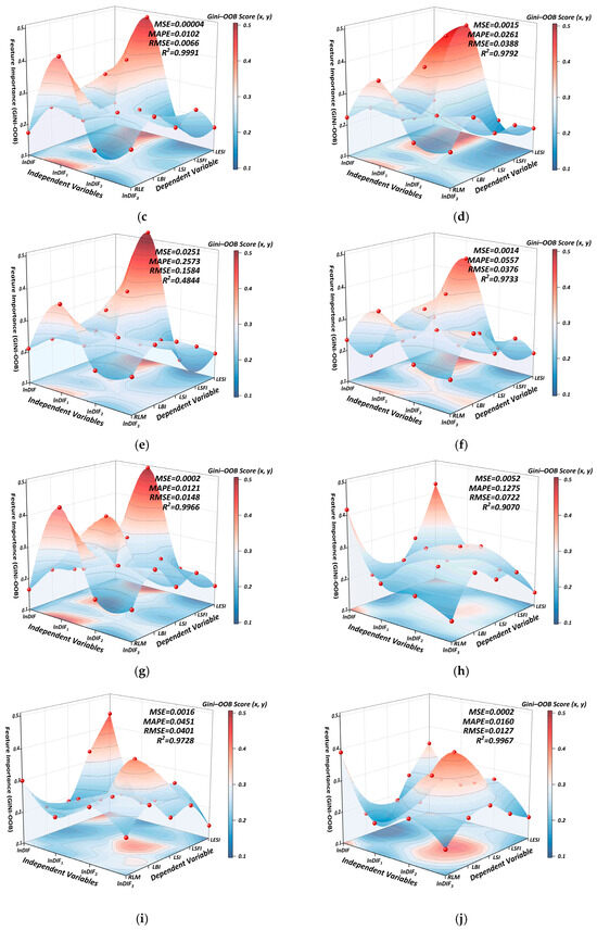
Figure 8. Yearly Feature Importance for RLM (2014–2023). (a) 2014, (b) 2015, (c) 2016, (d) 2017, (e) 2018, (f) 2019, (g) 2020, (h) 2021, (i) 2022, (j) 2023.

Figure 8 provides a longitudinal view of the Gini–OOB feature importance surfaces for RLM prediction across 2014–2023. Overall, the composite importance scores range from 0.103 to 0.514, showing moderate fluctuations over the decade. Notably, the influence of lnDIF₁ on RLM remains consistently high across all years, while lnDIF₃ exhibits persistently low importance, especially for LESI. Temporal dynamics indicate increasing differentiation after 2018, with lnDIF showing rising influence on LBI and RLM, suggesting a shifting emphasis from structural and fairness concerns toward behavioral and integrated market outcomes.

5. Conclusions and Policy Recommendations

The research develops an interpretable ensemble learning framework (PSO-GA-RF) to examine the nonlinear and dynamic effects of DIF on RLM outcomes in China. Using panel data from 58 counties in Jiangsu Province from 2014 to 2023, we construct a four-dimensional RLM indicator system encompassing labor behavior, structural adjustment, equity assurance, and economic sustainability. The empirical results demonstrate that DIF influences the RLM through a stage-dependent mechanism with clear dimensional heterogeneity. Although our empirical focus is on Jiangsu, a province with relatively advanced digital infrastructure and institutional capacity, the three-stage mechanism and the four-dimensional RLM framework provide a transferable template that can be adapted to other Chinese provinces and comparable developing economies. However, we also note that the magnitude of the estimated DIF effects in Jiangsu is likely to represent an upper bound relative to less-developed regions, and coefficients and thresholds should be recalibrated with local data before drawing policy conclusions elsewhere.

Specifically, from 2014 to 2016, DIF’s impact was predominantly “access-driven”, as infrastructure expansion and account penetration played foundational roles in facilitating labor participation. Between 2017 and 2020, the mechanism shifted to “usage-deepening”, where increased engagement with digital credit, mobile payments, and online financial tools reshaped employment behavior and income diversification. Since 2021, the digitalization dimension of DIF has shown rising marginal effects, particularly in labor structure and equity outcomes, suggesting an emerging “structure-integrating” phase, although its broader influence remains constrained by infrastructural and institutional limitations.

These findings offer several practical implications for policy. First, DIF development should be strategically phased: expanding access in early stages, fostering usage engagement in the medium term, and supporting structural integration in the long run. Second, improving digital financial literacy and platform governance is essential to reduce usage barriers and avoid digital exclusion, especially among vulnerable populations. Finally, DIF should be integrated into broader rural policy frameworks, including entrepreneurship support, skills training, and social protection programs, to create a synergistic “finance–skills–employment” loop. Such integration can enhance employment resilience, promote inclusive labor transitions, and unlock the full potential of DIF in advancing rural revitalization and broader economic, environmental, and institutional sustainability.

Despite these contributions, this study has several limitations that should be acknowledged. First, the empirical analysis is confined to 58 counties in Jiangsu Province, so the external validity of our findings to less-developed provinces or other developing economies remains to be tested. Second, the RLM and DIF indices, although auditable and theoretically grounded, are constrained by available county-level administrative data and cannot fully capture micro-level job quality, informal employment, or environmental externalities. Third, the PSO-GA-RF framework mainly uncovers nonlinear associations rather than fully causal effects, and we do not explicitly model long-run general equilibrium feedbacks or policy shocks. These limitations point to several promising avenues for future research, including cross-provincial or cross-country comparisons, the use of household- or transaction-level microdata to link DIF usage with individual labor trajectories and environmental outcomes, and the integration of causal machine learning or structural models to identify more robust policy channels.

References

- Lee, H.; Kim, T.B. The effectiveness of labor market indicators for conducting monetary policy: Evidence from the Korean economy. Econ. Model. 2023, 118, 106098. [Google Scholar] [CrossRef]
- Costa, L.; Teixeira, J.R. Structural change with different consumption profiles in a pure labour economy. Struct. Change Econ. Dyn. 2018, 47, 28–34. [Google Scholar] [CrossRef]
- United Nations Human Settlements Programme (UN-Habitat). World Cities Report. 2022: Envisaging the Future of Cities; United Nations: Nairobi, Kenya, 2022. Available online: https://unhabitat.org/wcr/2022/ (accessed on 16 November 2025).
- Feuerbacher, A.; McDonald, S.; Dukpa, C.; Grethe, H. Seasonal rural labor markets and their relevance to policy analyses in developing countries. Food Policy 2020, 93, 101875. [Google Scholar] [CrossRef]
- Li, L. An empirical analysis of rural labor transfer and household income growth in China. J. Chin. Hum. Resour. Manag. 2023, 14, 106–116. [Google Scholar] [CrossRef]
- Wei, B.; Zhao, C.; Luo, M. Online markets, offline happiness: E-commerce development and subjective well-being in rural China. China Econ. Rev. 2024, 87, 102247. [Google Scholar] [CrossRef]
- Liu, X. Research on rural human resources development from the perspective of rural revitalization. J. Southwest Minzu Univ. 2023, 44, 216–224. [Google Scholar]
- Jin, J. Financial supply for rural revitalization strategy. Finance Econ. 2024, 7–10. [Google Scholar]
- Zhou, H.; Nie, F.; Li, S.; Zhu, H. Sustainable development of assisted industries under the rural revitalization strategy: Status, problems, and countermeasures. Think Tank Theory Pract. 2023, 8, 8–18. [Google Scholar]
- Chen, H. The employment dilemma and human base of the development of modern agricultural industry. J. China Agric. Univ. 2024, 41, 33–47. [Google Scholar]
- Gao, Q.; Sun, M.; Chen, L. The impact of digital inclusive finance on agricultural economic resilience. Financ. Res. Lett. 2024, 66, 105679. [Google Scholar] [CrossRef]
- Hong, X.; Chen, Q.; Wang, N. The impact of digital inclusive finance on the agricultural factor mismatch of agriculture-related enterprises. Financ. Res. Lett. 2024, 59, 104774. [Google Scholar] [CrossRef]
- Li, E.; Tang, Y.; Zhang, Y.; Yu, J. Mechanism research on digital inclusive finance promoting high-quality economic development: Evidence from China. Heliyon 2024, 10, e25671. [Google Scholar] [CrossRef]
- Song, X.L. Empirical test on the narrowing urban–rural income gap by digital inclusive finance. Financ. Sci. 2017, 6, 14–25. [Google Scholar]
- Yi, X.J.; Li, Z. Does the development of digital inclusive finance significantly affect residents’ consumption? Micro evidence from Chinese families. J. Financ. Res. 2018, 11, 47–67. [Google Scholar]
- Zhao, H.; Chen, S.; Zhang, W. Does digital inclusive finance affect urban carbon emission intensity: Evidence from 285 cities in China. Cities 2023, 142, 104552. [Google Scholar] [CrossRef]
- Jiao, Y.; Wang, G.; Li, C.; Pan, J. Digital inclusive finance, factor flow and industrial structure upgrading: Evidence from the Yellow River basin. Financ. Res. Lett. 2024, 62, 105141. [Google Scholar] [CrossRef]
- Li, Y.; Jin, G.; Cui, Z.; Lv, B.; Xu, Z. Does digital inclusive finance promote regional green inclusive growth? Financ. Res. Lett. 2024, 62, 105163. [Google Scholar] [CrossRef]
- Bu, Y.; Du, X.; Wang, Y.; Liu, S.; Tang, M.; Li, H. Digital inclusive finance: A lever for SME financing? Int. Rev. Financ. Anal. 2024, 93, 103115. [Google Scholar] [CrossRef]
- Munyegera, G.K.; Matsumoto, T. Mobile Money, remittances, and household welfare: Panel evidence from rural Uganda. World Dev. 2016, 79, 127–137. [Google Scholar] [CrossRef]
- Dittus, P.; Klein, M.U. On harnessing the potential of financial inclusion. SSRN Electron. J. 2011. [Google Scholar] [CrossRef]
- Kelikume, I. Digital financial inclusion, informal economy and poverty reduction in Africa. J. Enterprising Communities People Places Glob. Econ. 2021, 15, 626–640. [Google Scholar] [CrossRef]
- Polloni-Silva, E.; Da Costa, N.; Moralles, H.F.; Sacomano Neto, M. Does financial inclusion diminish poverty and inequality? A panel data analysis for Latin American countries. Soc. Indic. Res. 2021, 158, 889–925. [Google Scholar] [CrossRef] [PubMed]
- Tran, H.T.T.; Le, H.T.T. The impact of financial inclusion on poverty reduction. Asian J. Law Econ. 2021, 12, 95–119. [Google Scholar] [CrossRef]
- Beck, T.; Demirgüç-Kunt, A.; Levine, R. Finance, inequality and the poor. J. Econ. Growth 2007, 12, 27–49. [Google Scholar] [CrossRef]
- Chibba, M. Inclusive development in Asia: Raison d’être and approaches. J. Asian Public Policy 2009, 2, 105–110. [Google Scholar] [CrossRef]
- Ozili, P.K. Impact of digital finance on financial inclusion and stability. Borsa Istanb. Rev. 2018, 18, 329–340. [Google Scholar] [CrossRef]
- Park, C.; Mercado, R. Financial inclusion, poverty, and income inequality. Singap. Econ. Rev. 2018, 63, 185–206. [Google Scholar] [CrossRef]
- Bachas, P.; Gertler, P.; Higgins, S.; Seira, E. Digital financial services go a long way: Transaction costs and financial inclusion. AEA Pap. Proc. 2018, 108, 444–448. [Google Scholar] [CrossRef]
- Akhter, S.; Liu, Y.; Daly, K. Cross country evidence on the linkages between financial development and poverty. Int. J. Bus. Manag. 2009, 5, 3. [Google Scholar] [CrossRef]
- Giller, K.E.; Delaune, T.; Silva, J.V.; Descheemaeker, K.; van de Ven, G.; Schut, A.G.; van Wijk, M.; Hammond, J.; Hochman, Z.; Taulya, G.; et al. The future of farming: Who will produce our food? Food Secur. 2021, 13, 1073–1099. [Google Scholar] [CrossRef]
- Gao, J.; Song, G.; Sun, X.Q. Does labor migration affect rural land transfer? Evidence from China. Land Use Policy 2020, 99, 105096. [Google Scholar] [CrossRef]
- Ma, W.L.; Zhou, X.S.; Renwick, A. Impact of off-farm income on household energy expenditures in China: Implications for rural energy transition. Energy Policy 2019, 127, 248–258. [Google Scholar] [CrossRef]
- Sibhatu, K.T.; Krishna, V.V.; Qaim, M. Production diversity and dietary diversity in smallholder farm households. Proc. Natl. Acad. Sci. USA 2015, 112, 10657–10662. [Google Scholar] [CrossRef]
- Tian, L. Land use dynamics driven by rural industrialization and land finance in the pen-urban areas of China: The examples of Jiangyin and Shunde. Land Use Policy 2015, 45, 117–127. [Google Scholar] [CrossRef]
- Zhang, H.; Li, J.; Quan, T.S. Strengthening or weakening: The impact of an aging rural workforce on agricultural economic resilience in China. Agriculture 2023, 13, 1436. [Google Scholar] [CrossRef]
- Steiner, A.; Atterton, J. Exploring the contribution of rural enterprises to local resilience. J. Rural Stud. 2015, 40, 30–45. [Google Scholar] [CrossRef]
- Deichmann, U.; Goyal, A.; Mishra, D. Will digital technologies transform agriculture in developing countries? Agric. Econ. 2016, 47, 21–33. [Google Scholar] [CrossRef]
- Rotz, S.; Gravely, E.; Mosby, I.; Duncan, E.; Finnis, E.; Horgan, M.; LeBlanc, J.; Martin, R.; Neufeld, H.T.; Nixon, A.; et al. Automated pastures and the digital divide: How agricultural technologies are shaping labour and rural communities. J. Rural Stud. 2019, 68, 112–122. [Google Scholar] [CrossRef]
- Chung, S.; Kim, K.; Lee, C.H.; Oh, W. Interdependence between online peer-to-peer lending and cryptocurrency markets and its effects on financial inclusion. Prod. Oper. Manag. 2023, 32, 1939–1957. [Google Scholar] [CrossRef]
- Muhle-Karbe, J.; Wang, Z.; Webster, K. Stochastic liquidity as a proxy for nonlinear price impact. Oper. Res. 2024, 72, 444–458. [Google Scholar] [CrossRef]
- Cao, J. Digital inclusive finance and agricultural modernization: Theoretical logic and empirical testing. Stat. Decis. 2024, 40, 144–149. [Google Scholar]
- Niu, G.; Jin, X.S.; Wang, Q.; Zhou, Y. Broadband infrastructure and digital financial inclusion in rural China. China Econ. Rev. 2022, 76, 101853. [Google Scholar] [CrossRef]
- Li, W.; He, W.W. Revenue-increasing effect of rural e-commerce: A perspective of farmers’ market integration and employment growth. Econ. Anal. Policy 2024, 81, 482–493. [Google Scholar] [CrossRef]
- Li, C.Y.; Sha, Z.H.; Sun, T. Rural households’ internet use on common prosperity: Evidence from the Chinese Social Survey. Soc. Indic. Res. 2023, 170, 797–823. [Google Scholar] [CrossRef]
- Seyedmohammadi, J.; Sarmadian, F.; Jafarzadeh, A.A.; McDowell, R.W. Development of a model using matter element, AHP and GIS techniques to assess the suitability of land for agriculture. Geoderma 2019, 352, 80–95. [Google Scholar] [CrossRef]
- Liu, W.; Hui, L.; Lu, Y.; Tang, J. Developing an evaluation method for SCADA-controlled urban gas infrastructure hierarchical design using multi-level fuzzy comprehensive evaluation. Int. J. Crit. Infrastruct. Prot. 2020, 30, 100375. [Google Scholar] [CrossRef]
- Wu, X.; Hu, F. Analysis of ecological carrying capacity using a fuzzy comprehensive evaluation method. Ecol. Indic. 2020, 113, 106243. [Google Scholar] [CrossRef]
- Zhang, Y.; Wang, R.; Huang, P.; Wang, X.; Wang, S. Risk evaluation of large-scale seawater desalination projects based on an integrated fuzzy comprehensive evaluation and analytic hierarchy process method. Desalination 2020, 478, 114286. [Google Scholar] [CrossRef]
- Kennedy, J.; Eberhart, R. Particle swarm optimization. In Proceedings of the International Conference on Neural Networks (ICNN’95), Perth, WA, Australia, 27 November–1 December 1995; Volume 4, pp. 1942–1948. [Google Scholar]
- Holland, J.H. Adaptation in Natural and Artificial Systems: An Introductory Analysis with Applications to Biology, Control, and Artificial Intelligence; MIT Press: Cambridge, MA, USA, 1992. [Google Scholar]
- Biggs, M.; Hariss, R.; Perakis, G. Constrained optimization of objective functions determined from random forests. Prod. Oper. Manag. 2023, 32, 397–415. [Google Scholar] [CrossRef]
- Gutjahr, W.J. Fair and efficient vaccine allocation: A generalized Gini index approach. Prod. Oper. Manag. 2023, 32, 4114–4134. [Google Scholar] [CrossRef]
- Li, X.; Qin, B.D.; Luo, Y.Y.; Zheng, D. A differential privacy budget allocation algorithm based on out-of-bag estimation in random forest. Mathematics 2022, 10, 4338. [Google Scholar] [CrossRef]
- Zhao, Z.; Yun, S.; Jia, L.; Guo, J.; Meng, Y.; He, N.; Li, X.; Shi, J.; Yang, L. Hybrid VMD-CNN-GRU-based model for short-term forecasting of wind power considering spatio-temporal features. Eng. Appl. Artif. Intell. 2023, 121, 105982. [Google Scholar] [CrossRef]
- Cyberspace Administration of Jiangsu Province (Ed.) 2022 Digital Jiangsu Development Report; Jiangsu Provincial Government: Nanjing, China, 2022.
- Yao, C.; Zhen, F.; Xi, G.; Wei, X.; Xiao, X. Spatial pattern and influencing factors of high-quality development of the digital economy in Jiangsu Province. Resour. Sci. 2025, 47, 268–280. [Google Scholar]
- National Bureau of Statistics (NBS) of China; Survey Office of Rural Socioeconomic Survey (Eds.) China County Statistical Yearbook 2014–2023 (Township and County Volumes); China Statistics Press: Beijing, China, 2023.
- Jiangsu Provincial Bureau of Statistics; National Bureau of Statistics (NBS) Jiangsu Survey Team (Eds.) Jiangsu Statistical Yearbook 2014–2023; China Statistics Press: Beijing, China, 2023.
- Jiangsu Provincial Bureau of Statistics (Ed.) Jiangsu Rural Development Yearbook 2020–2023; China Statistics Press: Beijing, China, 2023.
- Jiangsu Provincial Bureau of Statistics (Ed.) Jiangsu Rural Statistics Yearbook 2014–2023; China Statistics Press: Beijing, China, 2023.
Disclaimer/Publisher’s Note: The statements, opinions and data contained in all publications are solely those of the individual author(s) and contributor(s) and not of MDPI and/or the editor(s). MDPI and/or the editor(s) disclaim responsibility for any injury to people or property resulting from any ideas, methods, instructions or products referred to in the content. |
© 2025 by the authors. Licensee MDPI, Basel, Switzerland. This article is an open access article distributed under the terms and conditions of the Creative Commons Attribution (CC BY) license (https://creativecommons.org/licenses/by/4.0/).