All for One or One for All? A Comparative Study of Grouped Data in Mixed-Effects Additive Bayesian Networks

Abstract

Additive Bayesian networks (ABNs) provide a flexible framework for modeling complex multivariate dependencies among variables of different distributions, including Gaussian, Poisson, binomial, and multinomial. This versatility makes ABNs particularly attractive in clinical research, where heterogeneous data are frequently collected across distinct groups. However, standard applications either pool all data together, ignoring group-specific variability, or estimate separate models for each group, which may suffer from limited sample sizes. In this work, we extend ABNs to a mixed-effect framework that accounts for group structure through partial pooling, and we evaluate its performance in a large-scale simulation study. We compare three strategies—partial pooling, complete pooling, and no pooling—cross a wide range of network sizes, sparsity levels, group configurations, and sample sizes. Performance is assessed in terms of structural accuracy, parameter estimation accuracy, and predictive performance. Our results demonstrate that partial pooling consistently yields superior structural and parametric accuracy while maintaining robust predictive performance across all evaluated settings for grouped data structures. These findings highlight the potential of mixed-effect ABNs as a versatile approach for learning probabilistic graphical models from grouped data with diverse distributions in real-world applications.

1. Introduction

Modeling complex multivariate dependencies is a central challenge in biomedical research and many other scientific fields. In practice, clinical and experimental datasets often contain variables of different types, including continuous, count, binary, and categorical, and are collected across multiple centers, hospitals, or experimental batches [1]. Such grouped data structures introduce additional complexity: observations within a group are typically more similar to each other than to observations from other groups, violating the independence assumptions of traditional statistical models [2,3]. Ignoring these dependencies can lead to biased parameter estimates, spurious relationships, and suboptimal predictive performance. On the other hand, analyzing each group separately can sacrifice statistical power and may produce unstable estimates, particularly when sample sizes are limited [4]. These challenges necessitate flexible modeling approaches that can accommodate mixed variable types while appropriately accounting for group-specific effects.

To this end, Additive Bayesian Networks (ABNs) have emerged as a powerful class of probabilistic graphical models [5,6,7,8,9,10]. ABNs extend traditional Bayesian Networks (BNs) by representing each variable’s dependency on its parents using a Generalized Linear Model (GLM) [11]. This structure provides a natural framework for handling mixed-type data, enabling the simultaneous modeling of continuous outcomes, count data, and categorical variables without resorting to information-losing transformations such as discretization [12]. The network’s structure is typically learned by searching for a model that optimizes a goodness-of-fit score, which can be derived from either a Bayesian or an information-theoretic (frequentist) perspective [11]. This flexibility, along with the ability to produce interpretable graphs of conditional independencies, makes ABNs particularly attractive. They are especially well-suited for settings where both statistical rigor and clarity are critical, such as in clinical datasets that include physiological measurements, laboratory results, and categorical patient characteristics.

Despite these advantages, standard ABN approaches are limited in their ability to handle grouped data. Typically, applications either pool all observations together, assuming a single homogeneous population, or fit separate networks for each group [4]. Complete pooling ignores potential heterogeneity between groups, potentially leading to biased estimates if group-specific effects exist. Conversely, no pooling may suffer from small sample sizes, resulting in unstable network structures and parameter estimates. Mixed-effects models offer a principled compromise by introducing partial pooling, allowing their parameters to vary across groups, while sharing information to improve estimation [3,13]. Integrating mixed-effects modeling within the ABN framework thus offers the potential to retain flexibility for mixed-type variables while accounting for group-specific deviations, a combination not available in standard ABN implementations.

Building on our previous work, which introduced mixed-effect ABNs for a clinical application [5,14], we now provide a comprehensive simulation study designed to formally quantify their performance. In our previous application [14], we demonstrated how mixed-effect ABNs can accommodate mixed-type variables and explicitly account for center-specific effects in real-world multicenter clinical data, yielding a more parsimonious network structure and improving predictive accuracy for outcomes with high inter-center variability compared to a standard pooled analysis. However, because that analysis was conducted on observational data, the true underlying network structure and parameter values were unknown. Consequently, performance assessment was limited to indirect metrics such as predictive accuracy and clinical plausibility. The present study provides the formal methodological validation that builds upon that initial application. Here, we design a comprehensive simulation study in which the ground-truth network structures, parameter values, and group-specific effects are prespecified and fully known. This simulation framework enables us to rigorously quantify the ability of mixed-effect ABN to recover true network structures, accurately estimate parameters, and make reliable predictions across a range of conditions, including varying sample sizes, network sparsity, and group configurations. By systematically exploring these scenarios, we aim to characterize the strengths and limitations of partial pooling in the ABN context and to provide practical guidance for their application in multicenter clinical studies.

2. Materials and Methods

2.1. Mixed-Effect Additive Bayesian Networks

BNs are structured probabilistic models that use directed acyclic graphs (DAGs) to encode dependencies between random variables. Each node represents a variable, while the edges describe direct probabilistic relationships among them. This structure facilitates the decomposition of complex joint distributions into simpler, local conditional distributions.

To accommodate complex multivariate data with a mixture of variable types (such as Gaussian, binomial, multinomial, and Poisson), the standard BN framework can be extended to ABNs. ABNs model the local distribution of each node using an appropriate GLM tailored to its distributional characteristics [11]. Within this framework, the conditional distribution of each node, given its parents, is specified through a link function that connects its expected value to a linear predictor composed of its parents. This allows for a unified modeling approach for heterogeneous data types within a single graphical model.

2.1.1. Modeling Grouped Data with Mixed-Effect Additive Bayesian Networks

In studies involving multiple data sources, such as multi-center clinical data, observations often exhibit inherent grouping. Ignoring this grouping, for instance, by treating all data as coming from a single population (complete pooling), can lead to biased parameter estimates and misleading graphical structures. Conversely, modeling each group independently (no pooling) prevents information sharing, which is particularly detrimental in settings with sparse or imbalanced samples [4].

To address this trade-off between complete and no pooling, we extend the ABN framework to incorporate mixed effects. This is achieved by replacing the GLMs with Generalized Linear Mixed-effects Models (GLMMs), thereby integrating hierarchical modeling directly into the BN structure. This approach enables partial pooling of information by varying model parameters (such as intercepts and slopes) in the local conditional models by group, capturing both fixed effects that are consistent across all groups and random effects that reflect group-specific deviations [4,14,15]. Formally, for a Gaussian node i, corresponding to the variable $X_i$, with parent set ${\Pi }_{X_i}=\{X_{i_1},X_{i_2},\dots \}$, the local conditional distribution can be written as:

$${\mathbf{X}}_i={\mu }_i{\mathbf{1}}_n+{\Pi }_{{\mathbf{X}}_i}{\beta }_i+{\mathbf{Z}}_i{\mathbf{b}}_i+{\epsilon }_i,{\mathbf{b}}_i\sim {\mathcal{N}}_r(\mathbf{0},{\Sigma }_i),{\epsilon }_i\sim {\mathcal{N}}_n(\mathbf{0},{\sigma }_i^2{\mathbf{I}}_n),$$

(1)

where ${\mu }_i$ is the intercept term, ${\beta }_i$ is a vector of fixed-effect coefficients, ${\Pi }_{{\mathbf{X}}_i}$ is the associated design matrix, and ${\epsilon }_i$ is the residual error. Grouping is represented by an additional categorical variable F, with each of the F related data sets supposed to be independent. The matrix ${\mathbf{Z}}_i$ is the random effects design matrix of size $n\times r$, with $r=(\left|{\Pi }_{X_i}\right|+1)\left|F\right|$, and the vector ${\mathbf{b}}_i$ represents the group-specific random effects and is independent of ${\epsilon }_i$.

2.1.2. Additive Bayesian Networks for Mixed Distribution Data

In this work, we restrict to random intercepts models, where only the intercept varies across groups. This choice balances modeling flexibility with computational tractability and interpretability [14]. While more complex random-effect structures, such as random slopes or interaction terms, can capture additional heterogeneity, they substantially increase model complexity and may lead to identifiability issues, particularly when working with high-dimensional networks or mixed discrete-continuous data [4]. The random intercept formulation still enables partial pooling and captures essential group-level variation in a sparser form, making it a practical and robust choice.

For a given node i and an observation $X_{ij}$ coming from group k, conditional on its parent set ${\Pi }_{X_i}$, the local model with a varying intercept can be written as:

$$g\left(\mathbb{E}\left[X_{ij}|{\left({\Pi }_{{\mathbf{X}}_i}\right)}_j,b_{k,i}\right]\right)={\mu }_i+{\left({\Pi }_{{\mathbf{X}}_i}\right)}_j{\beta }_i+b_{k,i},$$

(2)

where ${\left({\Pi }_{{\mathbf{X}}_i}\right)}_j$ is the jth row of the associated design matrix, $b_{k,i}\sim \mathcal{N}(0,{\sigma }_{b,i}^2)$ is the random intercept for group k, and g is the canonical link function for variable $X_i$, which depends on its distribution: identity link for Gaussian, logit link for binomial, multinomial logit for multinomial, and log link for Poisson.

2.1.3. Model Complexity

Building on the GLMM framework, we define a metric to quantify the complexity of the network structure, which is determined by the total number of parameters to be estimated. For the random-intercepts model described in Equation (2), the complexity for each node i is the sum of its fixed-effects, random-effects variance, and residual variance parameters:

$${\Theta }_{X_i}=\underset{\mathrm{Fixed}\mathrm{effects}}{\underbrace{1+|{\Pi }_{X_i}|}}+\underset{\text{Random-effect}\mathrm{variance}}{\underbrace{1}}+\underset{\mathrm{Residual}\mathrm{variance}}{\underbrace{1{\mathrm{I}}_{X_i\mathrm{is}\mathrm{Gaussian}}}}.$$

(3)

The fixed effects include one parameter for the overall intercept (${\mu }_i$) and one for each parent in ${\Pi }_{X_i}$. The random-effect component consists of a single variance parameter, ${\sigma }_{b,i}^2$, for the random intercept. An additional parameter for the residual variance is included only for Gaussian nodes. Note that this formulation is a simplification of the more general model in Scutari et al. [4], which also includes random slopes and their full covariance matrix. Summing over all nodes in the graph, we obtain the total model complexity:

$$\Theta =\sum _{i=1}^p{\Theta }_{X_i}=2p+\sum _{i=1}^p\left|{\Pi }_{X_i}\right|+p_{\mathcal{N}},$$

(4)

where $p_{\mathcal{N}}$ is the number of Gaussian nodes in the DAG.

2.1.4. Structure Learning and Parameter Estimation in Mixed-Effect ABNs

Learning the structure of a BN with mixed effects involves identifying the optimal set of directed edges that best represent conditional dependencies among variables while accounting for hierarchical grouping. The inclusion of random effects increases the number of parameters and the complexity of the model space, as covariance parameters for random effects must be estimated alongside fixed-effect coefficients.

To manage this complexity, we use score-based structure learning algorithms that optimize penalized likelihood criteria, such as the Bayesian Information Criterion (BIC), adapted for GLMMs. For this methodological evaluation, we chose an exact search algorithm because it guarantees finding the optimal network structure, thereby providing the most reliable and unambiguous baseline for assessing model performance. While this approach is not scalable to high-dimensional data [16], the mixed-effects ABN framework is fully compatible with approximate, heuristic search algorithms (e.g., hill-climbing or genetic algorithms) that are suitable for larger networks. Specifically, we use exact search methods [16] to identify network structures that balance goodness-of-fit and parsimony. Parameter estimation for each candidate local model is performed within a maximum likelihood framework, using random intercepts to model group-level variation.

To evaluate the effects of accounting for grouped data structures, we compare our mixed-effect model, known as partial pooling ($PP$), with two common alternative approaches. The first, complete pooling ($CP$), ignores the grouping variable and learns a single model from the entire dataset under the assumption of homogeneity. The second approach, no pooling ($NP$), treats the data from different groups as completely independent. Although one could achieve this by training a separate network for each group, a more integrated solution is to incorporate the grouping variable as a fixed-effect covariate within a single model. We employ this latter approach by designating the grouping variable as a parent of every other node in the network. This stratified model ensures that the parameters for each node are conditioned on group identity, effectively preventing the sharing of information across groups while maintaining a cohesive and comparable model structure. Finally, we validate the resulting network structure for each approach through bootstrapping to assess the stability and reliability of the inferred connections.

All analyses were performed using the R package abn [17], which is designed for structure learning and parameter estimation in ABNs.

2.2. Simulation Study

To evaluate the performance of the mixed-effect ABN algorithm under various settings, we conducted a comprehensive simulation study with varying DAG structures, variable types, sample sizes, and grouping scenarios.

2.2.1. DAG Generation

We first generated multiple DAGs with the following characteristics:

• Number of nodes $p\in \{3,6,9,12\}$;
• Sparsity level $s\in \{0.2,0.4,0.6\}$, which defines the proportion of possible edges, yielding a number of ${\displaystyle \frac{p(p-1)}{2}}\times s$ edges.

For each combination of $(p,s)$, five distinct DAGs were created by randomly removing edges from a fully connected DAG until the desired sparsity level was reached.

For a consistent measure of network complexity across the simulation settings, a single complexity value for each explored setting $(p,s)$ was defined by applying Equation (4), replacing the actual number of parents $|{\Pi }_{X_i}|$, which varies across the generated graphs, by the average number of parents per node in the graph, denoted $\overline{\Pi }$. This average number of parents per node was calculated as the number of edges divided by the total number of nodes in the graph:

$$\overline{\Pi }={\displaystyle \frac{\frac{p(p-1)}{2}\times s}{p}}={\displaystyle \frac{s(p-1)}{2}}.$$

(5)

2.2.2. Data Simulation

For each of the generated DAGs, we simulated datasets with a total of $n\in \{100,250,500,1000,2000\}$ observations and p variables, denoted $X_1,\dots ,X_p$, corresponding to the p nodes in the graph. The observations were split into $k\in \{2,5,10,20\}$ groups based on four distinct group-size configurations:

• Even: Equal group sizes $\overline{n}=n/k$;
• $1S$: One small group of size $0.5\times \overline{n}$ and $k-1$ large groups, with the remaining observations distributed equally among them;
• $1L$: One large group of size $1.5\times \overline{n}$ and $k-1$ small groups, with the remaining observations distributed equally among them;
• $HSHL$: Half of the groups are small (size $0.25\times \overline{n}$) and the other half are large, with the remaining observations distributed equally among them.

Each dataset was simulated in accordance with the mixed-effect ABN framework, described in Section 2.1.2. For each node, values were drawn from a conditional distribution defined by a GLMM (see Equation (2)) with the appropriate canonical link function. We considered four different distributions across nodes:

• Balanced: Variables are equally distributed among Gaussian, binomial, multinomial;
• Gaussian: One binomial, one multinomial, with all others being Gaussian;
• Binomial: One Gaussian, one multinomial, with all others being binomial;
• Multinomial: One Gaussian, one binomial, with all others being multinomial.

Although ABNs can accommodate count data via Poisson-family GLMMs, we excluded Poisson variables from this simulation study due to practical challenges in both data generation and model fitting. First, simulating realistic count data presents challenges due to the necessity of addressing overdispersion, a prevalent deviation from the equi-dispersion assumption of the Poisson model, which significantly complicates the data-generating process [18]. Second, fitting Poisson GLMMs relies on numerical integration methods (e.g., Laplace approximation) to approximate the likelihood, as no closed-form solution exists [3]. These methods can exhibit numerical instability and convergence failures, particularly with sparse data or low counts. To ensure robust and consistent model fitting across the thousands of scenarios in our study, we prioritized stability and deferred the inclusion of Poisson variables for future work.

Multinomial variables were generated with three to five discrete levels, randomly selected for each simulation.

Both intercept terms and regression coefficients for parent nodes were independently sampled from a uniform distribution on $(0,2]$. To incorporate hierarchical group-level structure, random effects were added as specified in Section 2.1. For Gaussian and binomial nodes, the random effect standard deviations were independently drawn from a uniform $(0,1]$ distribution. For multinomial nodes, the random effects for the $C-1$ categories (with C the total number of categories for that node) were drawn from a multivariate normal distribution with zero mean and a covariance matrix generated to introduce correlations among category-level random effects. This covariance matrix was estimated from a sample of 1000 draws from a multivariate normal distribution with a zero mean and an identity covariance of dimension $C-1$.

To optimize computational resources, redundant simulations were avoided. Specifically, for settings with $k=2$, the $1S$, $1L$, and $HSHL$ group-size configurations are mathematically equivalent configurations. Likewise, for p = 3 nodes, the Gaussian, Binomial, and Multinomial node compositions are identical to the Balanced setup. Therefore, results were reused for these equivalent cases to ensure consistency without re-running identical experiments.

All data were simulated using rjags, using custom model specifications for each variable type and network structure [19,20].

2.2.3. Parameters of the Algorithm

For the structure learning phase, we employed an exact search algorithm to identify the optimal network structure, as implemented in the R package abn. The search was constrained by setting a maximum number of parents (max.parents) ranging from 2 to 4 per node to balance computational feasibility with the need to explore sufficient structural possibilities. This value was chosen for each unique setting of nodes (p) and sparsity (s) by taking the average number of parents $\left(\overline{\Pi }\right)$ in the graph, as defined in Section 2.2.1, and rounding up to the nearest integer:

$$\mathrm{max.parents}=\lceil \overline{\Pi }\rceil =⌈{\displaystyle \frac{s(p-1)}{2}}⌉.$$

(6)

To ensure the search was not overly stringent, the minimum effective max.parents was set to 3, provided this value did not exceed the total number of possible parents ($p-1$).

The BIC, adapted for generalized linear mixed-effects models, served as the score function to guide the search, balancing model fit against complexity. These settings were held constant across all pooling strategies (partial pooling, complete pooling, and no pooling) to ensure a fair comparison. For details, we refer the readers to the Github code repository at github.com/furrer-lab/mabnsimstud (accessed on 29 September 2025).

2.2.4. Summary of Simulation Settings

Table 1 and Table 2 summarize the performed simulations. For statistical stability and reliable inference, simulations in which at least one group had fewer than 25 observations were excluded. This threshold is informed by established guidelines for multilevel modeling, which indicate that while parameter estimates may remain unbiased with smaller group sizes, standard error estimation and random-effect variance components require adequate within-group sample sizes for stability [18,21,22]. Given the complexity of our mixed-distribution framework and the use of exact search algorithms for structure learning, we adopt a conservative threshold of 25 observations per group to ensure robust estimation of both fixed effects and random-effect variance components across all variable types. This threshold ensures that each group provides sufficient information for stable maximum likelihood estimation while maintaining computational feasibility for exact structure learning. Additionally, we did not consider situations where the chosen sparsity level s was too low to ensure a single connected DAG.

Table 1. Number of samples per group for each simulation. Gray numbers correspond to simulations that were excluded from the analysis. Numbers are rounded to the nearest integer. For the unbalanced configurations $1S$, $1L$, and $HSHL$, the minimum and maximum group sizes are presented in brackets.

		Sample Size (n)
	Groups ($\mathit{k}$)	100	250	500	1000	2000
$Even$	2	50	125	250	500	1000
	5	20	50	100	200	400
	10	10	25	50	100	200
	20	5	13	25	50	100
$1S$	2	(25, 75)	(62, 188)	(125, 375)	(250, 750)	(500, 1500)
	5	(10, 23)	(25, 56)	(50, 113)	(100, 225)	(200, 450)
	10	(5, 11)	(13, 26)	(24, 53)	(50, 106)	(100, 211)
	20	(3, 5)	(6, 13)	(13, 26)	(25, 51)	(50, 103)
$1L$	2	(25, 75)	(62, 188)	(125, 375)	(250, 750)	(500, 1500)
	5	(18, 30)	(44, 75)	(88, 150)	(175, 300)	(350, 600)
	10	(9, 15)	(24, 38)	(47, 75)	(94, 150)	(189, 300)
	20	(5,8)	(12, 19)	(24, 38)	(49, 75)	(97, 150)
$HSHL$	2	(25, 75)	(62, 188)	(125, 375)	(250, 750)	(500, 1500)
	5	(13, 25)	(31, 63)	(63, 125)	(125, 250)	(250, 500)
	10	(5, 15)	(13, 38)	(25, 75)	(50, 150)	(100, 300)
	20	(3, 8)	(6, 19)	(13, 38)	(25, 75)	(50, 150)

Table 2. Average number of edges (rounded to the nearest integer) and maximum number of parents (max.parents) for each simulation setting. Gray numbers indicate simulations excluded from the analysis because a connected DAG could not be guaranteed.

	Number of Nodes (p)
Sparsity ($\mathit{s}$)	3	6	9	12
Average edges
0.2	1	3	7	13
0.4	1	6	14	26
0.6	2	9	22	40
max.parents
0.2	-	-	-	3
0.4	-	3	3	3
0.6	2	3	3	4

2.3. Model Evaluation

We evaluated the performance of the algorithm using four distinct criteria:

• Structural accuracy, measured by the Structural Hamming Distance (SHD) between the learned DAG and the true data-generating DAG.
• Parametric accuracy, assessed using the Kullback–Leibler (KL) divergence between the learned and true conditional probability distributions for each node.
• Prediction error, evaluated using a 5-fold cross-validation procedure. To specifically isolate the accuracy of parameter estimation, a single consensus DAG was first learned from the full dataset. The model parameters were re-estimated on the training set, and the prediction error was calculated on the held-out test set. The error was then computed as the average of the differences between observed and predicted values across all nodes, more specifically:

  -

  For Gaussian distributed nodes $X_i$, we use the Mean Squared Error (MSE):

  $${\displaystyle \frac{1}{n}}\sum _{j=1}^n{({\widehat{X}}_{ij}-X_{ij})}^2,\mathrm{where}{\widehat{X}}_{ij}=\widehat{\mathbb{E}}\left(X_{ij}\right).$$

  (7)

  -

  For binomial distributed nodes $X_i$, we use the Brier score, which measures the mean squared difference between the predicted probability and the observed binary outcome:

  $${\displaystyle \frac{1}{n}}\sum _{j=1}^n{({\widehat{p}}_{ij}-X_{ij})}^2,\mathrm{where}{\widehat{p}}_{ij}=\widehat{\mathbb{P}}(X_{ij}=1).$$

  (8)

  -

  For multinomial distributed nodes $X_i$, we use the multi-category Brier score:

  $${\displaystyle \frac{1}{n}}\sum _{j=1}^n\sum _{c=1}^C{({\widehat{p}}_{ij,c}-1{\mathrm{I}}_{X_{ij}=c})}^2,$$

  (9)

  where ${\widehat{p}}_{ij,c}=\widehat{\mathbb{P}}(X_{ij}=c)$ and C is the number of categories.

  The final prediction error is the average of these scores across all nodes and all five test folds, yielding a single predictive accuracy score for each simulation.
• Computational efficiency, measured by the total runtime (in minutes) of the algorithm from structure learning to parameter estimation.

3. Results

3.1. Mixed-Effect Additive Bayesian Networks and Their Parameter Behavior

In this section, we evaluate the performance of the mixed-effect ABN algorithm under various conditions. Our analysis is structured in two parts: first, we investigate the effects of the number of observations (n), the number of groups (k), and the distribution of the groups; second, we analyze the impact of structural properties by varying the number of nodes (p), the sparsity levels (s), and the distribution of the nodes.

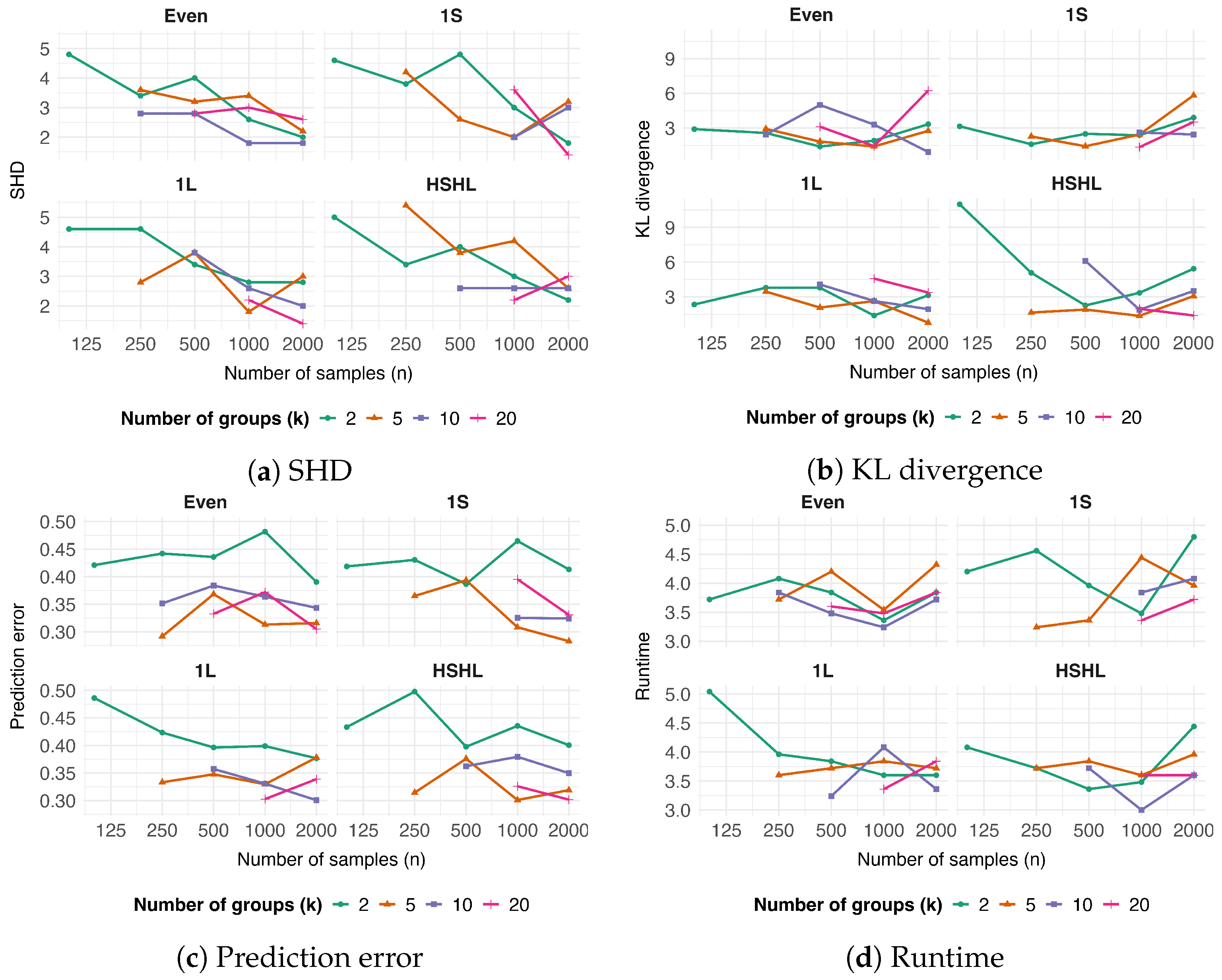
For the first analysis, we fix the number of nodes at $p=6$, the sparsity at $s=0.4$, and the node distribution to the Balanced configuration. These parameters were selected to provide a moderate and computationally feasible baseline for our analysis, allowing us to isolate and evaluate the effects of sample size and group structure. Performance results for SHD, KL divergence, prediction error, and runtime are shown in Figure 1.

Figure 1. Performance of the mixed-effect ABN algorithm as a function of sample size (n) and number of groups (k). Four performance metrics are shown: (a) Structural Hamming Distance (SHD), (b) Kullback–Leibler (KL) divergence, (c) prediction error, and (d) runtime in minutes. In each sub-figure, the x-axis represents the total number of samples (n). Line colors denote the number of groups ($k=2,5,10,20$). The four sub-panels correspond to different group-size configurations, which describe how the total number of samples is allocated among the available groups: Even (all groups have the same number of samples), 1S (one group is small), 1L (one group is large), and HSHL (half the groups are small and half are large). Each measurement represents the average of five repetitions conducted on different DAG structures to ensure statistical reliability and robustness.

The SHD consistently decreased with increasing sample size (Figure 1a). This trend was observed across all tested group distributions (Even, $1S$, $1L$, and $HSHL$). In contrast to structural recovery, KL divergence, which measures parametric fit, was insensitive to changes in sample size or group structure (Figure 1b). The prediction error was not affected by the number of samples, but decreased as the number of groups k increased, with a notable drop in performance at $k=2$ (Figure 1c). Finally, the runtime of the mixed-effect ABN algorithm showed no discernible impact from variations in the number of samples, groups, or group distributions (Figure 1d).

Next, we investigate the effects of the graph’s structural properties on model performance. For this analysis, we fix the number of samples at $n=1000$, the number of groups at $k=5$, and the group distribution to the $Even$ configuration. These values were chosen to represent a typical dataset size and a balanced group structure, ensuring that the results reflect the impact of varying the number of nodes, sparsity, and nodes’ distribution. The results for SHD, KL divergence, prediction error, and runtime are presented in Figure 2.

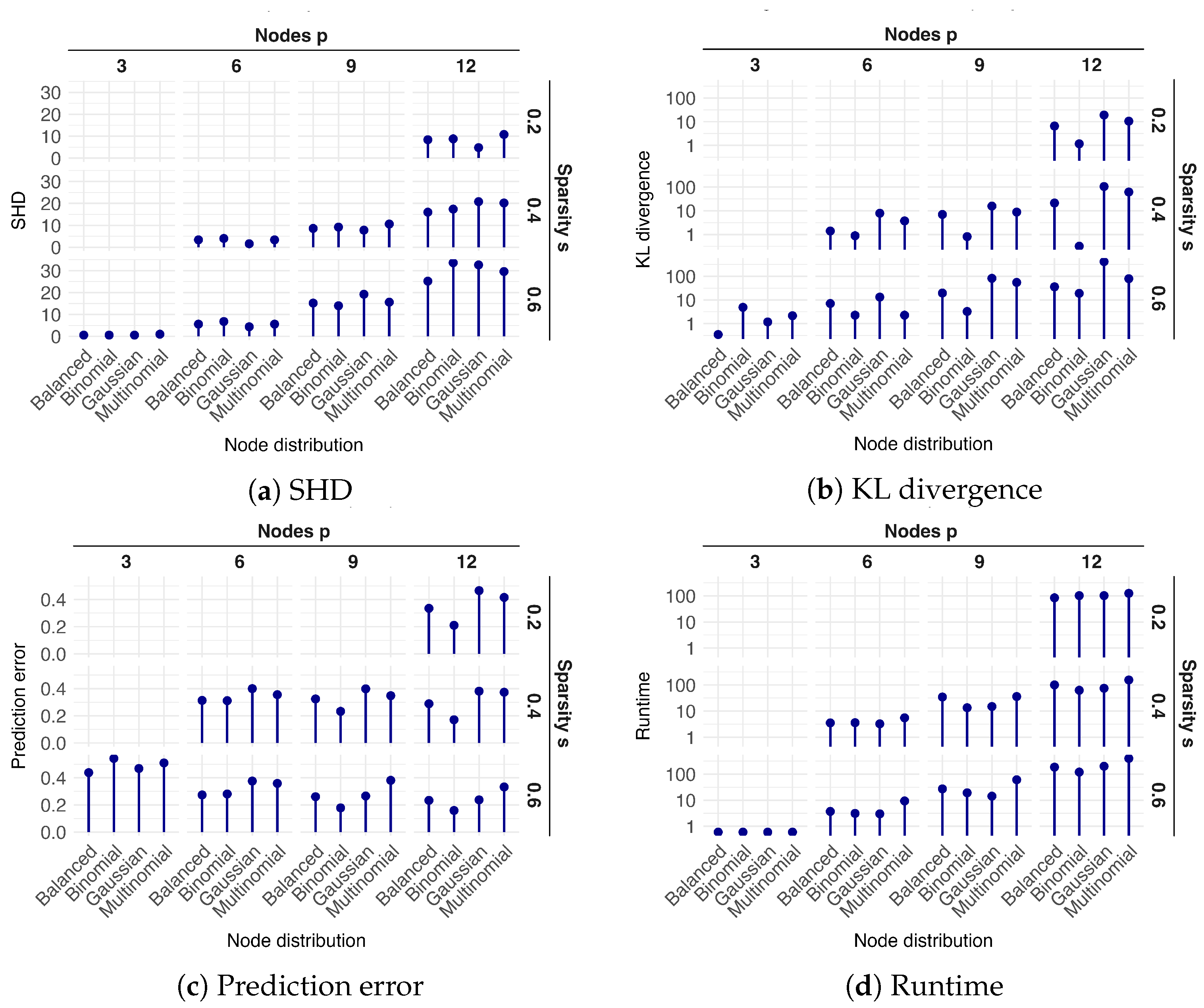
Figure 2. Performance of the mixed-effect ABN algorithm under varying graph structures, with each measurement averaged over five repetitions on distinct DAGs. The figure comprises four main panels, showing: (a) the Structural Hamming Distance (SHD), (b) the Kullback–Leibler (KL) divergence, (c) the prediction error, and (d) the runtime in minutes. Each main panel is organized as a grid, with columns representing the number of nodes (p) and rows representing the sparsity level (s). Within each individual cell of this grid, the results for four different node compositions are plotted along the x-axis: Balanced, with an even distribution of node types; and three specific configurations Binomial, Gaussian, and Multinomial, each containing one node of the other two types and the remaining nodes of the primary type.

The results for both SHD and KL divergence demonstrated a clear trend of increasing error as the number of nodes (p) and the sparsity (s) increased (Figure 2a,b). While performance varies across the different node distribution configurations ($Balanced$, $Binomial$, $Gaussian$, and $Multinomial$), no consistent ranking of these distributions was observed. Conversely, the prediction error decreased as the number of nodes (p) and graph sparsity (s) increased (Figure 2c). Finally, runtime increased significantly with the number of nodes (p), an effect that became more pronounced at higher sparsity levels (s) (Figure 2d).

3.2. Comparison with Pooling Strategies

In this section, we compare the performance of three distinct strategies for handling grouped data: complete pooling ($CP$), which assumes no group-level effects; no-pooling ($NP$), which treats each group independently; and partial pooling ($PP$), which uses random effects to share information across groups. The analysis is structured into two parts: first, we examine the impact of the number of samples per group; second, we evaluate how each strategy performs as graph complexity increases. This comparison aims to quantify the trade-offs between these modeling choices in terms of accuracy and computational cost.

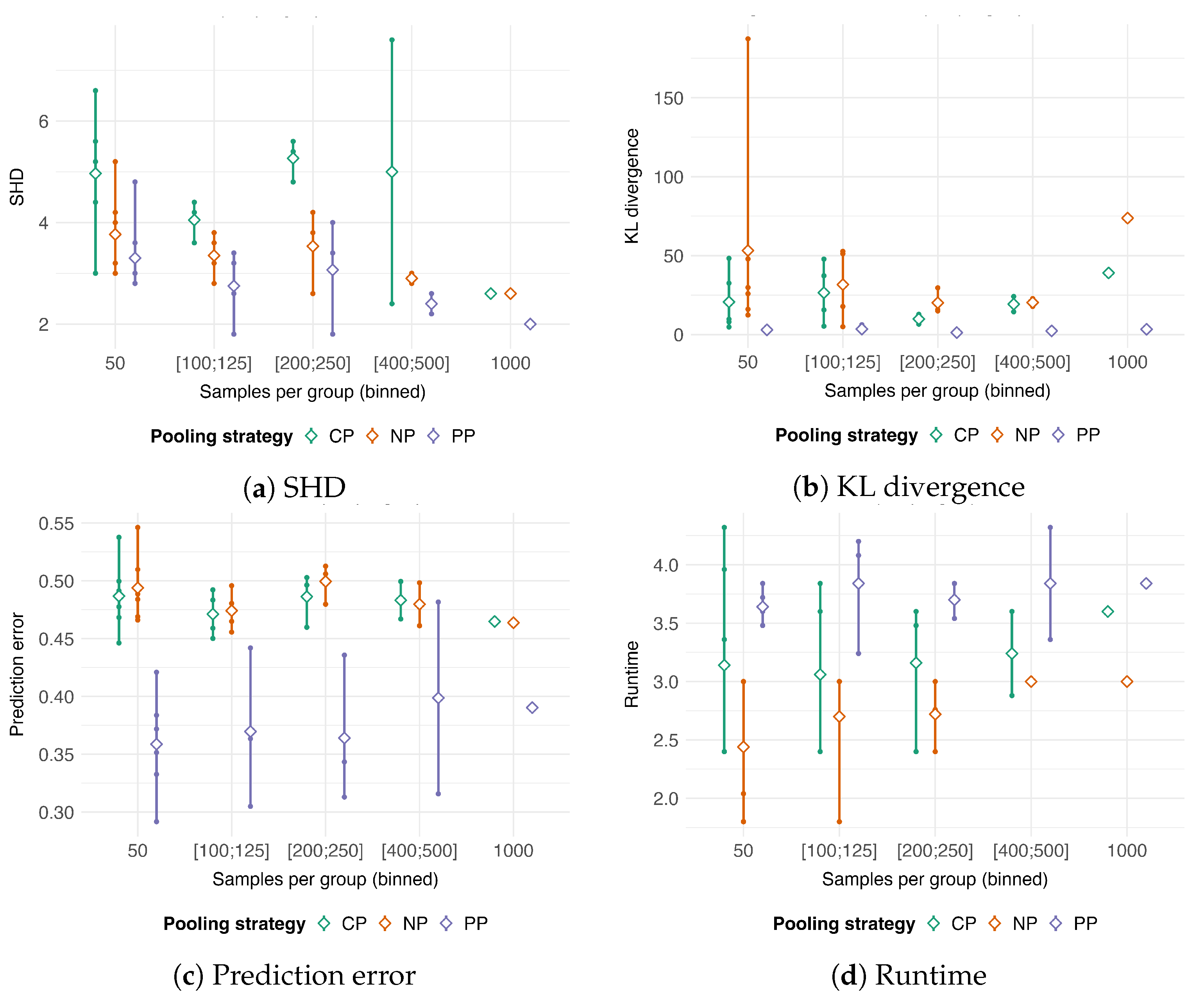
For the first analysis, we fix the number of nodes at $p=6$, the sparsity at $s=0.4$, the node distribution to $Balanced$, and the group-size configuration to $Even$. The $Even$ configuration was specifically selected to compare the impact of the number of samples per group across simulations, while the other parameters were set to ensure a good balance between computational feasibility and complexity. To simplify, we group the simulation settings into 5 categories based on the number of samples per group (see Table 1):

• 50, corresponding to the $(n=100,k=2)$, $(n=250,k=5)$, $(n=500,k=10)$ and $(n=1000,k=20)$ settings.
• $[100;125]$, corresponding to the $(n=250,k=2)$, $(n=500,k=5)$, $(n=1000,k=10)$ and $(n=2000,k=20)$ settings.
• $[200;250]$, corresponding to the $(n=500,k=2)$, $(n=1000,k=5)$ and $(n=2000,k=10)$ settings.
• $[400;500]$, corresponding to the $(n=1000,k=2)$ and $(n=2000,k=5)$.
• 1000, corresponding to the $(n=2000,k=2)$ setting.

We then measure the SHD, KL divergence, prediction error, and runtime as presented in Figure 3.

Figure 3. Performance comparison of complete pooling ($CP$), no-pooling ($NP$), and partial pooling ($PP$) strategies as a function of the number of samples per group. To isolate the effect of group size, results from multiple simulation settings (combinations of total sample size n and number of groups k) are aggregated into discrete bins based on the approximate number of samples per group, which are displayed on the x-axis. The pooling strategies represent distinct approaches to handling grouped data: (1) $CP$ assumes homogeneity, with no group-specific effects; (2) $NP$ treats group membership as a fixed effect, estimating parameters separately for each group; and (3) $PP$ uses random effects to enable partial information sharing across groups. The panels show boxplots for four performance metrics: (a) Structural Hamming Distance (SHD), (b) Kullback–Leibler (KL) divergence, (c) prediction error, and (d) runtime (in minutes). A unique color distinguishes each pooling strategy.

In terms of SHD, structural recovery improved across all strategies with increasing sample numbers per group (Figure 3a). Overall, $PP$ consistently yielded the lowest SHD, while $CP$ produced the highest. Note that, for the 1000-samples-per-group setting, only one dataset was available for this configuration ($n=2000$ and $k=2$). In terms of KL divergence, $NP$ resulted in the highest error, while $PP$ was the most accurate (Figure 3b). Prediction error for $PP$ was consistently lower than for $CP$ and $NP$ (Figure 3c). However, the variance of the error for $PP$ was substantially higher, influenced by the case with only two groups ($k=2$). Runtime was unaffected by the number of samples per group for all three methods (Figure 3d). $NP$ had the lowest median runtime, and $PP$ was the most computationally intensive.

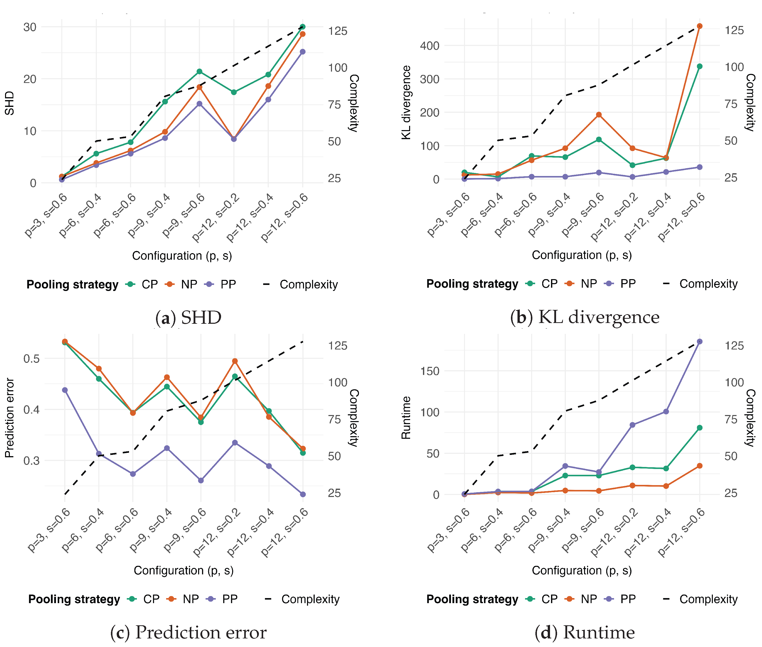
Next, we evaluate the performance of the three pooling strategies in relation to the graph’s complexity. For this analysis, we fix the number of samples to $n=1000$, the number of groups to $k=5$, the group-size configuration to $Even$, and the node distribution to the $Balanced$ configuration, to provide a typical and controlled data environment. Performance results, in terms of SHD, KL divergence, prediction error, and runtime, are presented in Figure 4.

Figure 4. Performance comparison of pooling strategies across varying levels of graph complexity. The strategies compared are: complete pooling ($CP$), which ignores group structure; no pooling ($NP$), which treats groups as independent fixed effects; and partial pooling ($PP$), which uses random effects to share information across groups. Graph complexity (dashed line, right y-axis), defined in Equation (4), increases with the number of nodes (p) and sparsity (s) of the network. The four panels show performance (left y-axis) based on: (a) Structural Hamming Distance (SHD), (b) Kullback–Leibler (KL) divergence, (c) prediction error, and (d) runtime in minutes. A unique color distinguishes each pooling strategy.

In terms of SHD, all methods were negatively affected by the graph’s complexity, though $PP$ consistently showed slightly better performance than $CP$ and $NP$ (Figure 4a). The KL divergence of $PP$ was minimally affected by complexity, whereas it increased substantially for $CP$ and $NP$ with increasing sparsity (Figure 4b). As previously observed, prediction error decreased with increasing graph complexity for all three strategies (Figure 4c), with $PP$ consistently achieving the lowest prediction error. Finally, the runtime of all methods increased with complexity; this effect was most pronounced for $PP$, while $NP$ remained the fastest method (Figure 4d).

4. Discussion

In this study, we conducted a comprehensive simulation to evaluate the performance of a mixed-effect ABN model and compare strategies for handling grouped data. Our findings provide strong empirical support for the use of partial pooling ($PP$) via random effects as a robust and accurate method for both structural learning and prediction in the presence of two-level hierarchical data structures.

4.1. Comparative Performance of Pooling Strategies

Our results demonstrate that the $PP$ strategy consistently outperforms complete pooling ($CP$) and no-pooling ($NP$) across nearly all evaluation metrics. This empirical confirmation supports the theoretical advantages of mixed-effects models, which balance the bias–variance trade-off by enabling partial information sharing across groups. This approach has proven effective for both continuous and discrete data, as shown by Scutari et al. [4], who utilized mixed-effects models for Gaussian networks, and Azzimonti et al. [15], who developed a hierarchical score for improved structure learning in discrete networks. The $CP$ model, which assumes data homogeneity, generated biased structural estimates, which is consistent with the known pitfalls of ignoring data heterogeneity [4]. In contrast, the $NP$ model treated groups independently, resulting in higher variance and reduced efficiency in learning shared patterns, a limitation that hierarchical models are designed to overcome [4,15]. For practitioners in fields where data are frequently clustered by hospital, laboratory, or region, these findings underscore the critical importance of selecting a pooling strategy that properly accounts for underlying group structures to avoid erroneous conclusions.

The prediction error results further highlight the advantages of the $PP$ approach. While the performance of $CP$ and $NP$ is quite similar, $PP$ consistently provides the lowest error (Figure 3c), which is critical in decision-support applications where predictive accuracy is paramount. However, $PP$ also exhibited substantially higher variance in its prediction error. This can be attributed to simulations with only two groups ($k=2$), as a very small number of groups can negatively affect the stability of random-effect estimates and thus increase prediction error, as shown in Figure 1c. For the $NP$ and $CP$ strategies, prediction error decreases with an increase in the number of samples per group. This trend is less apparent for $PP$, which maintains a consistently low error regardless of the number of samples, further underscoring its efficiency in learning from grouped data.

One key finding of this study is the behavior of the mixed-effect ABN algorithm as graph complexity increases. The accuracy of the $PP$ strategy remained superior as networks grew larger and denser. This robustness is crucial for real-world applications, where the underlying networks comprise many variables and their associations. The observed decrease in average prediction error with increasing network size can be attributed to a dilution effect, in which individual node-specific errors are masked when averaged across the entire network. Consequently, for effective decision-making, it is advisable to assess prediction accuracy at specific nodes of substantive importance, rather than relying solely on a global average. Our findings also confirmed that prediction errors in mixed-effect models decrease with a greater number of groups, consistent with established principles that more groups provide more information to accurately estimate the random effects distribution [22].

The analysis also reveals a clear and practical trade-off between model accuracy and computational cost. The superior performance of the $PP$ strategy comes at the price of increased computational time, particularly for more complex networks. In contrast, the $NP$ model was consistently the fastest. This trade-off is a crucial consideration for real-world applications. For analyses where accuracy is paramount, the $PP$ strategy is clearly the preferred choice for grouped data. However, for applications requiring real-time inference or analysis of extremely large networks, the faster $NP$ or $CP$ approaches might serve as pragmatic alternatives, provided that their potential limitations in accuracy are acknowledged.

4.2. Limitations

Our study has several limitations that present opportunities for future research. Firstly, our simulations were performed under idealized conditions, where the data-generating process strictly adhered to the model assumptions. Future investigations should assess the robustness of these methods when assumptions are violated, for example, by incorporating non-Gaussian or skewed distributions for the random effects. Secondly, evaluating prediction performance across heterogeneous data types is challenging due to the lack of a unified metric. The prediction errors reported for Gaussian, binomial, and multinomial nodes are therefore not directly comparable, underscoring the importance of a standardized evaluation framework (see also Appendix C). Thirdly, while we examined a broad range of parameters, the effect of the number of groups (k) deserves closer scrutiny, particularly at the lower threshold where estimating the variance of random effects becomes unstable. Our findings showed a decline in performance at $k=2$, which is consistent with the existing literature [22], but a more detailed analysis of this threshold would be advantageous. Furthermore, this simulation study focused solely on networks involving Gaussian, binomial, and multinomial nodes. Although Poisson models are compatible with the ABN framework for mixed-effects under maximum likelihood estimation, integrating them into the Bayesian data simulation approach proved challenging due to complexities in achieving stable and effective estimates. Future work should focus on incorporating Poisson-distributed nodes to broaden the applicability of mixed-effect ABNs to a wider range of count data challenges. Finally, expanding this framework to include dynamic Bayesian networks could offer a powerful method for analyzing longitudinal clustered data.

5. Conclusions

This study provides a rigorous quantitative validation of the mixed-effect ABN framework. By demonstrating its superior accuracy in structural recovery and prediction for grouped data, we establish it as a powerful and reliable tool for researchers and decision-makers dealing with complex, hierarchical systems. The primary contribution of this work is the empirical confirmation that accounting for group-level heterogeneity is a critical component for robust inference in Bayesian networks with mixed variable distributions. The clear elucidation of the accuracy-computation trade-off further provides practical guidance for its implementation, ensuring that the appropriate pooling strategy can be selected to meet the specific needs of a given scientific or industrial application.

References

1. Spiegelhalter, D.; Abrams, K.; Myles, J. Bayesian Approaches to Clinical Trials and Health-Care Evaluation; Wiley: Hoboken, NJ, USA, 2004. [Google Scholar]
2. Gelman, A.; Hill, J. Data Analysis Using Regression and Multilevel/Hierarchical Models; Analytical Methods for Social Research; Cambridge University Press: Cambridge, UK, 2006. [Google Scholar]
3. McCulloch, C.; Searle, S.R.; Neuhaus, J. Generalized, Linear and Mixed Models, 2nd ed.; Wiley Series in Probability and Statistics; Wiley: Hoboken, NJ, USA, 2008. [Google Scholar]
4. Scutari, M.; Marquis, C.; Azzimonti, L. Using Mixed-Effects Models to Learn Bayesian Networks from Related Data Sets. In Proceedings of the 11th International Conference on Probabilistic Graphical Models, Almeria, Spain, 5–7 October 2022; pp. 73–84. [Google Scholar]
5. Delucchi, M.; Spinner, G.R.; Scutari, M.; Bijlenga, P.; Morel, S.; Friedrich, C.M.; Furrer, R.; Hirsch, S. Bayesian network analysis reveals the interplay of intracranial aneurysm rupture risk factors. Comput. Biol. Med. 2022, 147, 105740. [Google Scholar] [CrossRef] [PubMed]
6. Hartnack, S.; Springer, S.; Pittavino, M.; Grimm, H. Attitudes of Austrian Veterinarians towards Euthanasia in Small Animal Practice: Impacts of Age and Gender on Views on Euthanasia. BMC Vet. Res. 2016, 12, 26. [Google Scholar] [CrossRef] [PubMed]
7. McCormick, B.J.J.; Sanchez-Vazquez, M.J.; Lewis, F.I. Using Bayesian Networks to Explore the Role of Weather as a Potential Determinant of Disease in Pigs. Prev. Vet. Med. 2013, 110, 54–63. [Google Scholar] [CrossRef] [PubMed]
8. Guinat, C.; Comin, A.; Kratzer, G.; Durand, B.; Delesalle, L.; Delpont, M.; Guérin, J.L.; Paul, M.C. Biosecurity risk factors for highly pathogenic avian influenza (H5N8) virus infection in duck farms, France. Transbound. Emerg. Dis. 2020, 67, 2961–2970. [Google Scholar] [CrossRef] [PubMed]
9. Aggrey, S.; Egeru, A.; Kalule, J.B.; Lukwa, A.T.; Mutai, N.; Hartnack, S. Household Satisfaction with Health Services and Response Strategies to Malaria in Mountain Communities of Uganda. Trans. R. Soc. Trop. Med. Hyg. 2025, 119, 85–96. [Google Scholar] [CrossRef] [PubMed]
10. Kowalska, M.E.; Shukla, A.K.; Arteaga, K.; Crasta, M.; Dixon, C.; Famose, F.; Hartnack, S.; Pot, S.A. Evaluation of Risk Factors for Treatment Failure in Canine Patients Undergoing Photoactivated Chromophore for Keratitis—Corneal Cross-Linking (PACK-CXL): A Retrospective Study Using Additive Bayesian Network Analysis. BMC Vet. Res. 2023, 19, 227. [Google Scholar] [CrossRef] [PubMed]
11. Kratzer, G.; Lewis, F.; Comin, A.; Pittavino, M.; Furrer, R. Additive Bayesian Network Modeling with the R Package abn. J. Stat. Softw. 2023, 105, 1–41. [Google Scholar] [CrossRef]
12. Scutari, M. Learning Bayesian Networks with the bnlearn R Package. J. Stat. Softw. 2010, 35, 1–22. [Google Scholar] [CrossRef]
13. Gelman, A.; Carlin, J.; Stern, H.; Dunson, D.; Vehtari, A.; Rubin, D. Bayesian Data Analysis, 3rd ed.; Chapman and Hall/CRC: Boca Raton, FL, USA, 2013. [Google Scholar]
14. Delucchi, M.; Bijlenga, P.; Morel, S.; Furrer, R.; Hostettler, I.; Bakker, M.; Bourcier, R.; Lindgren, A.; Maschke, S.; Bozinov, O.; et al. Mixed-effects Additive Bayesian Networks for the Assessment of Ruptured Intracranial Aneurysms: Insights from Multicenter Data. Comput. Biol. Med. 2025. submitted. [Google Scholar]
15. Azzimonti, L.; Corani, G.; Scutari, M. A Bayesian hierarchical score for structure learning from related data sets. Int. J. Approx. Reason. 2022, 142, 248–265. [Google Scholar] [CrossRef]
16. Koivisto, M.; Sood, K. Exact Bayesian Structure Discovery in Bayesian Networks. J. Mach. Learn. Res. 2004, 5, 549–573. [Google Scholar]
17. Delucchi, M.; Liechti, J.; Spinner, G.; Furrer, R. Additive Bayesian Networks. J. Open Source Softw. 2024, 9, 6822. [Google Scholar] [CrossRef]
18. Bolker, B.M.; Brooks, M.E.; Clark, C.J.; Geange, S.W.; Poulsen, J.R.; Stevens, M.H.H.; White, J.S.S. Generalized Linear Mixed Models: A Practical Guide for Ecology and Evolution. Trends Ecol. Evol. 2009, 24, 127–135. [Google Scholar] [CrossRef] [PubMed]
19. Lunn, D.; Spiegelhalter, D.; Thomas, A.; Best, N. The BUGS project: Evolution, critique and future directions. Stat. Med. 2009, 28, 3049–3067. [Google Scholar] [CrossRef] [PubMed]
20. Plummer, M.; Best, N.; Cowles, K.; Vines, K. CODA: Convergence Diagnosis and Output Analysis for MCMC. R News 2006, 6, 7–11. [Google Scholar]
21. Sagan, A. Sample Size in Multilevel Structural Equation Modeling—The Monte Carlo Approach. Econometrics 2019, 23, 63–79. [Google Scholar] [CrossRef]
22. Maas, C.; Hox, J. Sufficient sample sizes for multilevel modeling. Methodol. Eur. J. Res. Methods Behav. Soc. Sci. 2005, 1, 86–92. [Google Scholar] [CrossRef]
Disclaimer/Publisher’s Note: The statements, opinions and data contained in all publications are solely those of the individual author(s) and contributor(s) and not of MDPI and/or the editor(s). MDPI and/or the editor(s) disclaim responsibility for any injury to people or property resulting from any ideas, methods, instructions or products referred to in the content.
Article Metrics
Citations
Article Access Statistics
Multiple requests from the same IP address are counted as one view.