Training-Free Few-Shot Image Classification via Kernel Density Estimation with CLIP Embeddings

Abstract

Few-shot image classification aims to recognize novel classes from only a handful of labeled examples, a challenge in domains where data collection is costly or impractical. Existing solutions often rely on meta learning, fine tuning, or data augmentation, introducing computational overhead, risk of overfitting, or are not highly efficient. This paper introduces ProbaCLIP, a simple training-free approach that leverages Kernel Density Estimation (KDE) within the embedding space of Contrastive Language-Image Pre-training (CLIP). Unlike other CLIP-based methods, the proposed approach operates solely on visual embeddings and does not require text labels. Class-conditional probability densities were estimated from few-shot support examples, and queries were classified by likelihood evaluation, where Principal Component Analysis (PCA) was used for dimensionality reduction, compressing the dissimilarities between classes on each episode. We further introduced an optional bandwidth optimization strategy and a consensus decision mechanism through cross-validation, while addressing the special case of one-shot classification with distance-based measures. Extensive experiments on multiple datasets demonstrated that our method achieved competitive or superior accuracy compared to the state-of-the-art few-shot classifiers, reaching up to 98.37% accuracy in five-shot tasks and up to 99.80% in a 16-shot framework with ViT-L/14@336px. We proved our methodology by achieving high performance without gradient-based training, text supervision, or auxiliary meta-training datasets, emphasizing the effectiveness of combining pre-trained embeddings with statistical density estimation for data-scarce classification.

1. Introduction

Few-shot image classification, the task of recognizing new classes using only a limited number of labeled examples, has become a highly active research area, particularly in scenarios where labeled data is scarce, costly, or constantly evolving, and robust generalization is necessary. For instance, collecting extensive labeled data can be prohibitively expensive or impractical are medical diagnostics [1,2], industrial inspection [3,4], and other applications [5,6,7]. Traditionally, strategies such as data augmentation, transfer learning, and meta learning have been employed to overcome the scarcity of labeled samples. Among these, meta learning, which involves training models across numerous episodic tasks to quickly adapt to new tasks, has been extensively studied [8]. However, it often suffers from instability due to high sensitivity to architecture and hyper-parameters, as exemplified in work on model agnostic meta learning (MAML) [9], which addresses generalization issues by improving convergence and robustness across unseen tasks. Furthermore, meta learners can be biased toward meta-training tasks, affecting performance in novel domains, a concern addressed by task-oriented meta learning (TAML), which provides less biased and more adaptable initialization [10]. To avoid these challenges, recent research has proposed alternative few-shot strategies. For example, a recent study enhanced the generalization of few-shot learning by generating semantically consistent synthetic labels, improving the alignment between embeddings and class representations [11]. These developments collectively indicate the need to shift away from heavy meta learning pipelines toward lighter and more robust few-shot methodologies.

Recently, the advent of large vision-language models such as Contrastive Language-Image Pre-training (CLIP), introduced by OpenAI researchers, has revolutionized few-shot classification by leveraging joint image-text embeddings learned from vast internet-scale datasets [12] using two encoders, one for texts and the other for images. CLIP supports zero-shot generalization, enabling the classification of unseen classes without further training.

Following the introduction of CLIP, other competitors benefited from image-text embeddings to propose a competitive advantage in tasks such as zero-shot classification. Among them are ALIGN [13] by Google Research, FLAVA [14] by Facebook AI Research, and SigLIP [15] by Google DeepMind researchers. More recently, other methods were introduced, replacing the employment of a separate text embedding by the use of a Large Language Model (LLM) connected with a projector that handles the image embedding mechanism, a modification that allows not only image, but multi-modal context for LLMs [16]. Some examples that also involve researchers from big corporations are LLaVA [17], Qwen2-VL [18], and NVLM [19], respectively, from Microsoft, Alibaba Group, and Nvidia. However, when compared independently, CLIP-based variants still excel in tasks such as linear probing, zero-shot classification, and clustering [20,21].

However, its performance can often be further enhanced by adapting the embeddings or inference mechanisms for few-shot image classification. Several studies have proposed adapting CLIP with minimal or no training in the context of linear probing or few-shot learning. Kato et al. [22] introduced Proto-Adapter, a training-free approach that constructs prototypes from few-shot examples to facilitate efficient inference in the CLIP embedding space. Similarly, Peng et al. [23] proposed Semantic-Guided Visual Adaptation (SgVA-CLIP), employing cross-modal knowledge distillation to improve visual representations with minimal fine-tuning. These methods emphasize the effectiveness of leveraging CLIP’s embeddings without extensive model retraining.

Domain adaptation methods have also been explored within the context of CLIP-based few-shot classification. Sun et al. [24] developed an adversarial domain adaptation approach, aligning visual and textual embedding distributions to enhance cross-domain few-shot classification performance. Furthermore, multi-modal and transductive inference techniques have shown significant potential. Chen et al. [25] presented Multi-source Information Fusion (MIF), integrating multiple textual and visual cues for robust few-shot classification. Martin et al. [26] explored transductive inference, jointly refining predictions across unlabeled queries using probabilistic modeling in the embedding space, significantly boosting classification accuracy. In specialized applications, Zhang and Liu [3] used Bayesian optimization combined with the CLIP embeddings for efficient few-shot classification of crack images in industrial settings, highlighting the versatility of the CLIP embeddings when integrated with optimization-based methods.

Despite these advancements, many existing approaches introduce additional complexities through trainable components or sophisticated adaptation mechanisms. In contrast, this paper proposes a straightforward, training-free few-shot classification method that employs kernel density estimation within a condensed version of the CLIP embedding space that uses principal component analysis to highlight the most relevant dissimilarities between classes in a lower dimensional space. Our method, ProbaCLIP, estimates class-specific probability densities from the few available labeled examples, classifying query images by evaluating the likelihood of their embeddings under each estimated density. This novel approach leverages the inherent structure of CLIP’s pre-trained embeddings without requiring gradient-based training, prompt engineering, or auxiliary meta-training datasets. Moreover, we propose an optional scheme that further improves overall accuracy by searching for the best bandwidth parameter for KDE. An overview of ProbaCLIP is shown in Figure 1.

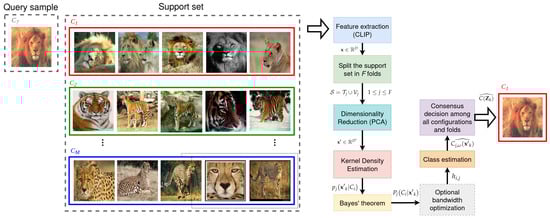
Figure 1. General overview of ProbaCLIP’s workflow illustrated with tieredImageNet image samples.

The contributions of this work are summarized as follows:

• Demonstration that simple statistical density estimation combined with dimensionality reduction can be applied to the CLIP embeddings to model class-conditional distributions, providing a probabilistic framework for few-shot classification and yielding results that are superior to or competitive with the state of the art.
• Illustration that effective few-shot classification can be achieved with the CLIP embeddings without gradient-based training, prompt engineering, or meta learning, or text embeddings, highlighting the efficiency and scalability of the approach in data-scarce scenarios.
• Analysis of the impact of the curse of dimensionality in the KDE framework with the CLIP embeddings and employment of PCA to mitigate it. The results show that dimensionality reduction significantly improves accuracy and plays a crucial role in interpreting meaningful patterns from a more specialized, higher-dimensional CLIP backbone.
• Introduction of an ensemble of multiple predictors constructed through a cross-validation scheme and optional strategies for KDE bandwidth optimization. These refinements further enhance the performance of the proposed methodology.

Together, these contributions establish that simple, statistically grounded techniques, when systematically combined with high-quality pre-trained embeddings, can surpass or rival recent state-of-the-art few-shot methods while drastically reducing computational cost and eliminating retraining.

This paper is organized as follows: Section 2 introduces the methodology proposed by our solution; Section 3 presents the obtained results and discussions, comparing our results with the state-of-the-art few-shot image classification models; and Section 4 presents the conclusions of the proposed method.

2. Proposed Solution

In few-shot classification, data is generally organized into episodes that simulate the low-data conditions encountered during testing. Each episode comprises a small number of classes (M) and a few labeled examples per class (N), forming what is known as an M-way N-shot problem. An episode includes two primary sets: support and query. The support set consists of N labeled examples for each of the M classes, while the query set contains multiple unlabeled examples from these same classes, used to evaluate the model’s ability to generalize.

Typically, during training, episodes are sampled from a meta-training set, which includes a wide range of classes and examples. For evaluation, episodes are drawn from a meta-test set comprising entirely unseen classes.

A key advantage of our approach is that it bypasses the need for a dedicated meta-training phase. Instead, the inference is performed directly using data from the meta-test set, which is partitioned into a support set ($\mathcal{S}$) and a query set ($\mathcal{Q}$). Here, $\mathcal{S}$ contains N examples per class across M novel classes, and $\mathcal{Q}$ holds the test examples associated with these classes used to measure performance.

Our approach consists of extracting embeddings of target images using a feature extractor. In this work, we focused on the pre-trained CLIP model due to its proven high performance, but it could be used with any other feature extraction model. At the end of this process, each image ${\mathbf{Z}}_{\alpha }$ was represented by a feature vector${\mathsf{\ell }}_{\alpha }{\mathbb{R}}^D$ with a few hundred dimensions depending on the CLIP backbone, where D is the number of dimensions.

To mitigate the curse of dimensionality, which refers to the performance degradation and increasing sparsity of data in high-dimensional feature spaces [27,28,29], we compressed the most important dissimilarities between the image classes into a lower-dimensional subspace using principal component analysis, as illustrated in Figure 2. Specifically, the number of target dimensions of each episode $D_e$ was set as the minimum number of principal components ($P{C}_{opt}$) that explain at least 99% of the variance of the training set whenever possible, provided that the total number of training samples ($N_t$) is greater than $P{C}_{opt}$ [30], as follows:

$$P{C}_{opt}=min\left\{PC\in \{1,\dots ,D\}|{\displaystyle \frac{{\sum }_{d=1}^{PC}{\mathrm{var}}_d}{{\sum }_{d=1}^D{\mathrm{var}}_d}}\ge 0.99\right\}$$

(1)

$$D_e=min(N_t,P{C}_{opt})$$

(2)

where ${\mathrm{var}}_d$ denotes the explained variance of the d-th principal component.

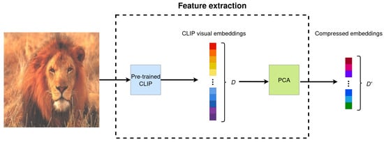
Figure 2. Illustration of the feature extraction process on an image sample of tieredImageNet dataset, where a pre-trained CLIP model was employed to extract image embeddings and PCA was used to reduce its number of dimensions.

When it was not possible to reach 99% of the explained variance with $P{C}_{opt}$, the first $PCs$ that accounted for the highest variance were selected. In this case, if the total explained variance was the same for $PC$ and $PC+1$, $P{C}_{opt}:=PC$ was set, which avoided adding components that did not contribute to explaining the variance of the subset. This choice of dimensionality reduction is consistent with theoretical studies on kernel estimators in functional spaces, which establish exact asymptotic error behavior and validate the robustness of kernel methods under subspace projection [31].

Another great advantage of using PCA is that it prevents multicollinearity by projecting the features in a space with orthogonal components, which are uncorrelated to each other. This is particularly important, considering that recent studies have shown that the CLIP embeddings reveal substantial mutual feature information when applied to multiclass classification, where the information contained in features of a particular class is significantly redundant with the information from features of other unrelated classes [32].

To enhance generalization, we performed cross-validation on $\mathcal{S}$, splitting it into F subsets. We chose $F=5$ so that there were five training subsets (${\mathcal{T}}_1,{\mathcal{T}}_2,\dots ,{\mathcal{T}}_5$) and five complementary validation subsets (${\mathcal{V}}_1,{\mathcal{V}}_2,\dots ,{\mathcal{V}}_5$), as the following:

$$\mathcal{S}={\mathcal{T}}_j\cup {\mathcal{V}}_j,{\mathcal{T}}_j\cap {\mathcal{V}}_j=⌀,1\le j\le F.$$

(3)

Figure 3 shows how the training and validation subsets are split depending on the split ratio between training and validation samples ($r_{split}$).

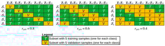
Figure 3. Cross–validation split between ${\mathcal{T}}_j$ and ${\mathcal{V}}_j$ for different values of $r_{split}$.

Although the dimension targeted for each episode ($D_e$) was determined using all the samples in $\mathcal{S}$, at each cross-validation iteration, PCA was performed separately only using the training subset ${\mathcal{T}}_j$. Thus, the number of dimensions of each cross-validation iteration $D^{\prime }$ was further reduced, as the number of samples in each episode was smaller than $N_t$. $D^{\prime }$ is defined as follows:

$$D^{\prime }=min(D_e,|{\mathcal{T}}_j\left|\right).$$

(4)

Then, a multidimensional kernel density estimate was performed with the extracted feature vectors with reduced dimension $D^{\prime }$ so that each class $C_i$ of the image classification problem, with $i\in \{1,\dots ,M\}$, was bound to a multidimensional probability density function (PDF). For simplicity, the Gaussian kernel was used in our experiments. The bandwidth used was the best fit for correctly assigning feature vectors to a PDF that corresponded to its class in the few-shot classification task.

Formally, the set of feature vectors $\{{\mathbf{x}}_1,\dots ,{\mathbf{y}}_1,\dots \}\in {\mathbb{R}}^D$ are represented as $\{{\mathbf{x}}_1^{\prime },\dots ,{\mathbf{y}}_1^{\prime },\dots \}\in {\mathbb{R}}^{D^{\prime }}$ after PCA transformation. Where, ${\mathbf{y}}_t^{\prime }$ are the feature vectors with subindex $t\in \left\{1,\dots ,|{\mathcal{T}}_j|\right\}$ belonging to ${\mathcal{T}}_j$ with known class labels, which are used to build up the probability density function of each class, while ${\mathbf{x}}_k^{\prime }$ are feature vectors from which the class labels are predicted. During the validation phase ${\mathbf{x}}_k^{\prime }\in {\mathcal{V}}_j$ and $k\in \left\{1,\dots ,|{\mathcal{V}}_j|\right\}$, while during the test phase ${\mathbf{x}}_k^{\prime }\in \mathcal{Q}$ and $k\in \left\{1,\dots ,\left|\mathcal{Q}\right|\right\}$. Then, $p\left({\mathbf{x}}_k^{\prime }|C_i\right)$, the class-conditional probability density of observing the transformed feature vector ${\mathbf{x}}_k^{\prime }$ given class $C_i$ is calculated with two different approaches at each iteration of the cross-validation scheme: using a unique scalar bandwidth $h_j$ in the KDE for the entire set $\mathcal{S}$, and with a scalar bandwidth $h_{i,j}$ for each class $C_i$ of the classification problem.

Considering a unique bandwidth for the entire set is the simplest approach for solving the kernel density estimation problem. In this case, given that $|{\mathcal{T}}_{i,j}|$ is the total number of elements in ${\mathcal{T}}_{i,j}$, which is a subset of ${\mathcal{T}}_j$ that contains only the elements of class $C_i$, the KDE for a test sample ${\mathbf{x}}_k^{\prime }$ takes the general form [33,34] as the following:

$$p_j({\mathbf{x}}_k^{\prime }\mid C_i)={\displaystyle \frac{1}{|{\mathcal{T}}_{i,j}|}}\sum _t^{|{\mathcal{T}}_{i,j}|}{\displaystyle \frac{1}{det{\left({\mathbf{H}}_j\right)}^{1/2}}}K\left({\mathbf{H}}_j^{-1/2}({\mathbf{x}}_k^{\prime }-{\mathbf{y}}_t^{\prime })\right)$$

(5)

where $K(·)$ is a kernel function in ${\mathbb{R}}^{D^{\prime }}$ and ${\mathbf{H}}_j$ is the positive definite bandwidth matrix that controls the smoothing intensity.

A common choice for K is the multivariate Gaussian kernel, which is adopted in our proposition as the following:

$$K\left(\mathbf{u}\right)={\left(2\pi \right)}^{-\frac{D^{\prime }}{2}}exp\left(-\frac{1}{2}{\mathbf{u}}^{\top }\mathbf{u}\right).$$

(6)

substituting (6) into (5) yields the following:

$$p_j({\mathbf{x}}_k^{\prime }\mid C_i)={\displaystyle \frac{1}{|{\mathcal{T}}_{i,j}|}}\sum _t^{|{\mathcal{T}}_{i,j}|}{\left(2\pi \right)}^{-\frac{D^{\prime }}{2}}det{\left({\mathbf{H}}_j\right)}^{-1/2}exp\left(-\frac{1}{2}{({\mathbf{x}}_k^{\prime }-{\mathbf{y}}_t^{\prime })}^{\top }{\mathbf{H}}_j^{-1}({\mathbf{x}}_k^{\prime }-{\mathbf{y}}_t^{\prime })\right).$$

(7)

Although PCA whitening was not applied, the PCA transformation already produced orthogonal (decorrelated) axes, making the isotropic assumption reasonable within the reduced feature space. Whitening was avoided to prevent the amplification of noise in low-variance directions, while isotropy was retained as an approximate assumption for simplicity and numerical stability. Considering that the bandwidth matrix is restricted to the isotropic case, ${\mathbf{H}}_j=h_j^2\mathbf{I}$ and $det\left({\mathbf{H}}_j\right)={\left(h_j^2\right)}^{D^{\prime }}$. Then, Equation (7) simplifies to the following equation:

$$p_j\left({\mathbf{x}}_k^{\prime }|C_i\right)={\displaystyle \frac{1}{|{\mathcal{T}}_{i,j}|{\left(h_j\sqrt{2\pi }\right)}^{D^{\prime }}}}\sum _t^{|{\mathcal{T}}_{i,j}|}exp\left(-{\displaystyle \frac{1}{2}}{\displaystyle \frac{{∥{\mathbf{x}}_k^{\prime }-{\mathbf{y}}_t^{\prime }∥}^2}{h_j^2}}\right)$$

(8)

where $∥.∥$ is the Euclidean norm and $h_j$ is the KDE bandwidth that can be found by an optional optimization algorithm that minimizes the classification error, or simply by assigning an initial guess $h_j^0$ to $h_j$. This algorithm and the formulation of $h_j^0$ are addressed in Section 2.2.

We also considered applying a different bandwidth for each image class such that Equation (8) can be rewritten as follows:

$$p_j\left({\mathbf{x}}_k^{\prime }|C_i\right)={\displaystyle \frac{1}{|{\mathcal{T}}_{i,j}|{\left(h_{i,j}\sqrt{2\pi }\right)}^{D^{\prime }}}}\sum _t^{|{\mathcal{T}}_{i,j}|}exp\left(-{\displaystyle \frac{1}{2}}{\displaystyle \frac{{∥{\mathbf{x}}_k^{\prime }-{\mathbf{y}}_t^{\prime }∥}^2}{h_{i,j}^2}}\right).$$

(9)

The only difference between Equations (8) and (9) is that the bandwidth $h_{i,j}$ depends on the class $C_i$ for the latter. In this case, the optimization described in Section 2.2 was performed separately for each class.

Then, Bayes’ theorem can be applied to Equations (8) and (9) to yield the probability that the image ${\mathbf{Z}}_k$ associated with feature vector ${\mathbf{x}}_k^{\prime }\in {\mathbb{R}}^{D^{\prime }}$ belongs to class $C_i$ as follows:

$$P_j\left(C_i|{\mathbf{x}}_k^{\prime }\right)={\displaystyle \frac{P_j\left(C_i\right)p_j\left({\mathbf{x}}_k^{\prime }|C_i\right)}{{\sum }_{q=1}^M{P}_j\left(C_q\right)p_j\left({\mathbf{x}}_k^{\prime }|C_q\right)}}$$

(10)

where $P_j\left(C_i\right)$ is the a priori probability of class $C_i$ in the cross-validation step j, which can be estimated from the training set as follows:

$$P_j\left(C_i\right)={\displaystyle \frac{|{\mathcal{T}}_{i,j}|}{|{\mathcal{T}}_j|}}.$$

(11)

Finally, the predicted class $\widehat{C_j\left({\mathbf{x}}_k^{\prime }\right)}$ for the image ${\mathbf{Z}}_k$ associated with the feature vector ${\mathbf{x}}_k^{\prime }$ in the cross-validation iteration j is the one with a maximum posteriori probability $P_j\left(C_i|{\mathbf{x}}_k^{\prime }\right)$ as follows:

$$\widehat{C_j\left({\mathbf{x}}_k^{\prime }\right)}=\underset{i\in \{1,\dots ,M\}}{arg\; max}{P}_j\left(C_i|{\mathbf{x}}_k^{\prime }\right).$$

(12)

2.1. AMISE-Based Bandwidth Selection for a d-Dimensional, Isotropic KDE

Consider ${\mathbf{X}}_1,\dots ,{\mathbf{X}}_n\in {\mathbb{R}}^d$ and the isotropic kernel density estimator with a single bandwidth $h>0$ and a product kernel $K_d$ as follows:

$${\widehat{f}}_h\left(\mathbf{x}\right)={\displaystyle \frac{1}{n{h}^d}}\sum _{i=1}^n{K}_d\left({\displaystyle \frac{\mathbf{x}-{\mathbf{X}}_i}{h}}\right),K_d\left(\mathbf{u}\right)=\prod _{j=1}^{d}K\left(u_j\right)$$

(13)

we define $R\left(g\right)$ and ${\mu }_2\left(K\right)=$ as follows:

$$R\left(g\right)={\int }_{{\mathbb{R}}^d}g{\left(\mathbf{x}\right)}^{2}d\mathbf{x},{\mu }_2\left(K\right)={\int }_{\mathbb{R}}{u}^{2}K\left(u\right)du.$$

(14)

For a product kernel built from the same univariate K, we have $R\left(K_d\right)={\left(R\left(K\right)\right)}^d$ and ${\mu }_2\left(K_d\right)={\mu }_2\left(K\right)$. Under the usual smoothness assumptions, the bias expansion yields the following [35,36]:

$$\mathrm{Bias}\left[{\widehat{f}}_h\left(\mathbf{x}\right)\right]={\displaystyle \frac{h^2}{2}}{\mu }_2\left(K\right)\Delta f\left(\mathbf{x}\right)+o\left(h^2\right)$$

(15)

where $\Delta f={\sum }_{j=1}^d{\partial }^{2}f/\partial x_j^2$ is the Laplacian. The integrated variance satisfies the following:

$$\int \mathrm{Var}\left[{\widehat{f}}_h\left(\mathbf{x}\right)\right]d\mathbf{x}={\displaystyle \frac{1}{n{h}^d}}R\left(K_d\right)+o\left({\displaystyle \frac{1}{n{h}^d}}\right).$$

(16)

Therefore, the Asymptotic MISE (AMISE) is defined as [35]:

$$\mathrm{AMISE}\left(h\right)={\displaystyle \frac{R\left(K_d\right)}{n{h}^d}}+{\displaystyle \frac{h^4}{4}}{\mu }_2{\left(K\right)}^{2}R\left(\Delta f\right),R\left(\Delta f\right)={\int }_{{\mathbb{R}}^d}{\left(\Delta f\left(\mathbf{x}\right)\right)}^{2}d\mathbf{x}$$

(17)

minimizing the AMISE over h gives the isotropic AMISE-optimal bandwidth, resulting in the following equation:

$$h_{\mathrm{AMISE}}={\left({\displaystyle \frac{dR\left(K_d\right)}{n{\mu }_2{\left(K\right)}^{2}R\left(\Delta f\right)}}\right)}^{{\displaystyle \frac{1}{d+4}}}.$$

(18)

A practical plug-in is the normal-reference (“rule-of-thumb”) choice obtained by approximating the unknown density by a spherical normal $N_d(\mu ,{\sigma }^2{I}_d)$ and using a Gaussian kernel. For the Gaussian kernel, $R\left(K_d\right)={\left(2^{-1}{\pi }^{-1/2}\right)}^d=2^{-d}{\pi }^{-d/2}$ and ${\mu }_2\left(K\right)=1$. Thus, $R\left(\Delta f\right)$ can be rewritten as the following:

$$R\left(\Delta f\right)=2^{-d}{\pi }^{-d/2}{\displaystyle \frac{\Gamma \left(\frac{d+4}{2}\right)}{\Gamma \left(\frac{d}{2}\right)}}{\sigma }^{-(d+4)}$$

(19)

substituting $R\left(\Delta f\right)$ into Equation (18) yields the multidimensional normal-reference bandwidth for the isotropic case as follows:

$$h_{\mathrm{NR}}(d,n)=\sigma {\left({\displaystyle \frac{d\Gamma \left(\frac{d}{2}\right)}{\Gamma \left(\frac{d+4}{2}\right)}}\right)}^{{\displaystyle \frac{1}{d+4}}}{n}^{-{\displaystyle \frac{1}{d+4}}}=\sigma {\left({\displaystyle \frac{4}{d+2}}\right)}^{{\displaystyle \frac{1}{d+4}}}{n}^{-{\displaystyle \frac{1}{d+4}}}.$$

(20)

This equation reduces to the Silverman’s rule for $d=1$. For simplicity, it can be written as follows:

$$h_{\mathrm{NR}}(d,n)=\sigma .\phi (d,n)$$

(21)

Considering a numerical example where $n=25$, inspired by five-way five-shot experiments and D dimensions, we found that $\phi (d,25)\approx 1$ was a good approximation for higher dimensions as shown in Figure 4, and used this approximation in all our experiments.

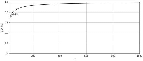
Figure 4. The plot of $\phi (d,n)$ for d between 25 and 1000 and $n=25$.

2.2. Bandwidth Optimization

Optional bandwidth optimization is performed to maximize classification accuracy for each iteration of the cross-validation scheme, where the bandwidth is optimized with the training set ${\mathcal{T}}_j$ and evaluated with the validation set ${\mathcal{V}}_j$. The optimization process used is an iterative gradient search that uses an optimizer with a loss function to search for the local minima of the bandwidth. We evaluated the Adam optimizer [37] together with two loss functions for this purpose. The first one is the Average Negative Log-Likelihood ($ANLL$) as the following:

$$ANLL=-{\displaystyle \frac{1}{|{\mathcal{T}}_j|}}\sum _{t=1}^{|{\mathcal{T}}_j|}log{P}_j\left(C_T|{\mathbf{y}}_t^{\prime }\right)$$

(22)

where $C_T$ is the true class for the training feature vector ${\mathbf{y}}_t^{\prime }$ and $P_j\left(C_T|{\mathbf{y}}_t^{\prime }\right)$ is the probability that the image associated with ${\mathbf{y}}_t^{\prime }$ belongs to class $C_T$. For simplicity, we use a notation that describes the application of the loss function to the training set ${\mathcal{T}}_j$; however, its application to the validation and test sets is analogous.

The second loss function is a variation of the $ANLL$, which we call the Modified Average Negative Log-Likelihood ($MANLL$). This loss function is calculated independently for each class, allowing the search for the optimal value of $h_{i,j}$ to be carried out with a different optimizer for each class as the following:

$$MANL{L}_i=-{\displaystyle \frac{1}{|{\mathcal{T}}_{i,j}|}}\sum _t^{|{\mathcal{T}}_{i,j}|}logp\left({\mathbf{y}}_t^{\prime }|C_i\right).$$

(23)

The gradient search for the optimal bandwidth value with Adam requires an initial value to start the optimization process. In this work, this value is set based on the empirical standard deviation of the data, motivated by the analysis described in Section 2.1. Thus, when accounting for a single bandwidth for the entire training set, the initial bandwidth value ($h_j^0$) is defined as follows:

$$h_j^0={\displaystyle \frac{1}{M}}\sum _{i=1}^M{\displaystyle \frac{1}{D^{\prime }}}tr\left(Cov\left({\mathcal{T}}_{i,j}\right)\right)$$

(24)

where $tr\left(.\right)$ is the trace operation, $Cov\left({\mathcal{T}}_{i,j}\right)$ is the covariance matrix of with dimensions $D^{\prime }\times D^{\prime }$ of the feature vectors contained in ${\mathcal{T}}_{i,j}$, and M denotes the total number of classes.

Similarly, when the initial bandwidth also depends on the class with index i, $h_{i,j}^0$ is defined as the following:

$$h_{i,j}^0={\displaystyle \frac{1}{D^{\prime }}}tr\left(Cov\left({\mathcal{T}}_{i,j}\right)\right).$$

(25)

As this optimization is an optional procedure, whenever it is not applied, the initial bandwidth values are chosen for KDE.

2.3. Consensus Decision with Cross-Validated Bandwidths

For each of the cross-validation iterations, a set $\mathcal{U}$ was assessed with four variations of our method, depending on the loss function and bandwidth optimization. These variations, namely $\mathcal{U}=\{u_1,u_2,u_3,u_4\}$, are described in Table 1. Each variation provides a particular estimate for each method, so that Equation (12) is modified as follows:

$$\widehat{C_{j,\omega }\left({\mathbf{x}}_k^{\prime }\right)}=\underset{i\in \{1,\dots ,M\}}{arg\; max}{P}_{j,\omega }\left(C_i|{\mathbf{x}}_k^{\prime }\right)$$

(26)

where $\omega \in \{1,2,3,4\}$ is the subindex of the variation belonging to $\mathcal{U}$, and $P_{j,\omega }\left(C_i|{\mathbf{x}}_k^{\prime }\right)$ is the probability of the class $C_i$ given the feature vector ${\mathbf{x}}_k^{\prime }$ for the cross-validation iteration j with the variation $u_{\omega }$ of our method.

Table 1. Configuration of the elements in $\mathcal{U}$.

Element in $\mathcal{U}$	Initial Bandwidth	Loss Function
$u_1$	$h_j^0$	$ANLL$
$u_2$	$h_j^0$	$MANLL$
$u_3$	$h_{i,j}^0$	$ANLL$
$u_4$	$h_{i,j}^0$	$MANLL$

Therefore, the proposed approach produced 20 class predictions for each image in the test phase, as there were four different estimates for each of the five iterations of the cross-validation scheme. At the end of the cross-validation iterations, the final class prediction for each image was the consensus among the ensemble of 20 predictors.

Then, the results of the optimal bandwidths obtained for each of the methods with the support set $\mathcal{S}$ (training and validation sets) were used to predict the image classes in the query set (test set) $\mathcal{Q}$. For each of the method variations and each of the cross-validation iterations, the predictions of all the test images in the query set are stored. At the end of this process, the predicted image is chosen as the consensus of majority vote among all the predictions as defined in Equation (27) as the following:

$$\widehat{C\left({\mathbf{Z}}_k\right)}=\underset{i\in \{1,\dots ,M\}}{arg\; max}\sum _{j=1}^F\sum _{\omega =1}^{\left|\mathcal{U}\right|}\mathbf{1}\left[\widehat{C_{j,\omega }\left({\mathbf{x}}_k^{\prime }\right)}=C_i\right]$$

(27)

where $\widehat{C\left({\mathbf{Z}}_k\right)}$ is the final consensus decision for the image ${\mathbf{Z}}_k$, and $\mathbf{1}\left[·\right]$ is the indicator function.

Although this proposition is intended to be employed for a few-shot image classification, it could be used to solve similar problems with very small datasets. Such datasets cannot be adequately managed by conventional image classification models because, even if the models are fine-tuned, they are likely to overfit the training set. On the other hand, the proposed model has a maximum of only M learnable parameters that are optional, namely the KDE bandwidths, so it is not likely to overfit.

2.4. Alternative Solution for One-Shot Image Classification

For the special case of an M-way one-shot problem, the KDE estimation method presented is not feasible because at least one sample should be used for training and another for validation within the same class. To solve this issue, we came up with another strategy to solve one-shot problems. Instead of predicting the class with KDE in a cross-validation scheme, we simply measure the distance between the test sample ${\mathbf{x}}_k^{\prime }\in \mathcal{Q}$ and each of the M samples ${\mathbf{y}}_t^{\prime }$. As each sample ${\mathbf{y}}_t^{\prime }\in \mathcal{S}$ belongs to a different class, the class of the image in which the shortest distance is measured is predicted as the image class as defined in Equation (28), as the following:

$$\widehat{C\left({\mathbf{Z}}_k\right)}=\underset{t\in \{1,\dots ,M\}}{arg\; min}dist({\mathbf{x}}_k^{\prime },{\mathbf{y}}_t^{\prime })$$

(28)

where $dist(·)$ represents the distance function. In this work, we evaluated cosine similarity and Euclidean distances.

3. Results and Discussions

We evaluated our proposition with three datasets that are commonly employed to few-shot learning: miniImageNet [38,39], tieredImageNet [40], and CUB200 2011 [41]. The choice of these datasets was convenient to compare the results obtained with other existing methods. These datasets were evaluated considering five-way one-shot and five-way five-shot tasks, which are also widely employed setups in few-shot learning papers. Then, Flowers102 [42], Food101 [43], Caltech101 [44], FGVC-Aircraft [45], and DTD [46] were employed as additional datasets in an extended evaluation to understand the robustness of our method under varied configurations (five-way one-shot, two-shot, four-shot, eight-shot, and sixteen-shot).

Furthermore, two CLIP Vision Transformer (ViT) backbones were evaluated for each of the datasets, namely ViT-B/32, which is claimed to be the fastest among the CLIP ViT backbones, and ViT-L/14@336px, which is a more powerful architecture with a slower inference time [12]. The feature vectors extracted with ViT-B/32 end up with $D=512$, while those extracted with ViT-L/14@336px have $D=768$. With both backbones, for five-shot experiments, a set of different $r_{split}=\{0.2,0.4,0.6,0.8\}$ was evaluated to determine the consensus among $\mathcal{U}$ and its individual performances. However, for one-shot experiments, as there are not enough samples for splitting $\mathcal{S}$ in $\mathcal{T}$ and $\mathcal{V}$, cosine similarity and Euclidean distance were assessed, as explained in Section 2.4.

All experiments were repeated for 1000 episodes for each configuration (except when stated otherwise), each time randomly selecting the M classes and the elements of $\mathcal{S}$. Then, the mean accuracy over the episodes was recorded to provide a better understanding of the overall robustness of our approach. Moreover, all the experiments were executed with and without dimensionality reduction to evaluate their impact on the final results.

The results of each of the experiments were stored without bandwidth optimization (training-free variant). Then, they were extended with the bandwidth search described in Section 2.2, which was executed for 500 iterations, where the Adam optimizer was set with a learning rate of 0.02, ${\beta }_1=0.9$, ${\beta }_1=0.999$, and weight decay $\lambda =0$.

3.1. Five-Way Five-Shot Experiments

First, the results of the proposed method for each of the configurations in $\mathcal{U}$ were individually assessed with five-way five-shot experiments without considering a cross-validation approach. In this case, only $\mathcal{S}={\mathcal{T}}_1\cup {\mathcal{V}}_1$ is evaluated so that we can use these results to understand the general impact of the cross-validation iterations in the proposed method. The results of this analysis using the CLIP ViT-B/32 backbone are shown in Figure 5a, Figure 5b and Figure 5c for miniImageNet, tieredImageNet, and CUB200 2011, respectively.

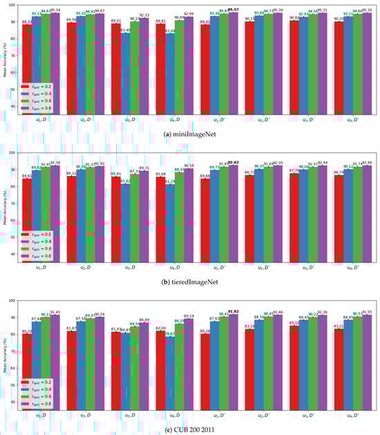
Figure 5. Mean results over 1000 episodes with bandwidth optimization for 500 iterations on a single iteration of the cross-validation scheme ($\mathcal{S}={\mathcal{T}}_1\cup {\mathcal{V}}_1$) with CLIP ViT-B/32 for $r_{split}=\{0.2,0.4,0.6,0.8\}$, where each group of bars represents a combination of the elements of $\mathcal{U}$ with D if the original dimension were employed, or $D^{\prime }$ if dimensionality reduction with PCA was employed. Also, the mean accuracy is displayed at the top of the bars. (a) MiniImageNet. (b) TieredImageNet. (c) CUB200 2011.

It is evident that dimensionality reduction plays an important role in our methodology, as experiments using compressed dimensions ($D\to D^{\prime }$) consistently outperformed those using the original dimensions.

In all variations, the best observed results were achieved for $r_{split}=0.8$. It indicates that for an approach that does not consider cross-validation, the more training samples available, the better to determine the initial bandwidth and to be used against the query set in the KDE paradigm.

Likewise, the same experiments were repeated with ViT-L/14@336px backbone. The results are plotted in Figure 6a, Figure 6b and Figure 6c for miniImageNet, tieredImageNet, and CUB200 2011, respectively. It is possible to observe that the impact of the loss function, bandwidth initialization, and dimensionality reduction for ViT-L/14@336px is similar to what is observed for ViT-B/32.

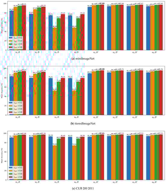
Figure 6. Mean results over 1000 episodes with bandwidth optimization for 500 iterations on a single iteration of the cross-validation scheme ($\mathcal{S}={\mathcal{T}}_1\cup {\mathcal{V}}_1$) with CLIP ViT-L/14@336px for $r_{split}=\{0.2,0.4,0.6,0.8\}$, where each group of bars represents a combination of the elements of $\mathcal{U}$ with D if the original dimension were employed, or $D^{\prime }$ if dimensionality reduction with PCA was employed. Also, the mean accuracy is displayed at the top of the bars. (a) MiniImageNet. (b) TieredImageNet. (c ) CUB200 2011.

However, a few observations stood out. First, ViT-L/14@336px achieved consistently better results than ViT-B/32 for all datasets evaluated with reduced dimensionality ($D^{\prime }$), demonstrating that compression of the information from a more advanced backbone yields superior performance. On the other hand, when comparing the backbones with their original dimensions (D), ViT-L/14@336px in some cases achieved worse performance than ViT-B/32. This observation highlights the importance of preferring a reduced number of dimensions to approach the KDE problem, where it is noticeable that a more advanced feature extraction that employs more dimensions could lead to worse performance if no dimensionality reduction technique is considered. Furthermore, ViT-L/14@336px achieved the best results with dimensionality reduction for all datasets on $u_1$.

Then, we repeated the experiments with cross-validation, where $1\le j\le 5$ and $\mathcal{S}={\mathcal{T}}_j\cup {\mathcal{V}}_j$ so that it was possible to calculate the consensus among each ($\widehat{C_{u_1}\left({\mathbf{x}}_k^{\prime }\right)}$, $\widehat{C_{u_2}\left({\mathbf{x}}_k^{\prime }\right)}$, $\widehat{C_{u_3}\left({\mathbf{x}}_k^{\prime }\right)}$, $\widehat{C_{u_4}\left({\mathbf{x}}_k^{\prime }\right)}$) and all ($\widehat{C\left({\mathbf{Z}}_k\right)}$) elements in $\mathcal{U}$. The results of this analysis employing CLIP ViT-B/32 backbone are shown in Figure 7a, Figure 7b and Figure 7c for miniImageNet, tieredImageNet, and CUB200 2011, respectively. While the results for ViT-L/14@336px are shown in Figure 8a, Figure 8b and Figure 8c for miniImageNet, tieredImageNet, and CUB200 2011, respectively.

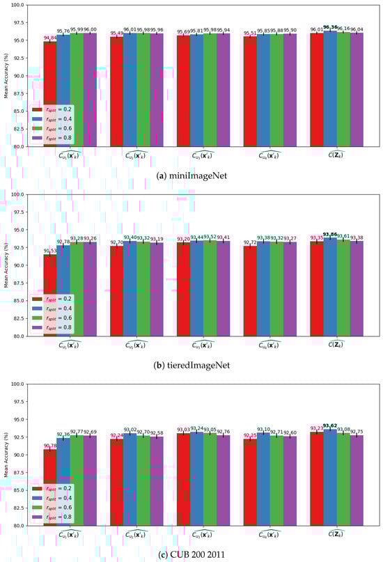
Figure 7. Mean results over 1000 episodes with bandwidth optimization for 500 iterations on cross-validations with CLIP ViT-B/32 feature vectors with reduced dimension $D^{\prime }$ for $r_{split}=\{0.2,0.4,0.6,0.8\}$, where $\widehat{C_{u_1}\left({\mathbf{x}}_k^{\prime }\right)}$, $\widehat{C_{u_2}\left({\mathbf{x}}_k^{\prime }\right)}$, $\widehat{C_{u_3}\left({\mathbf{x}}_k^{\prime }\right)}$, and $\widehat{C_{u_4}\left({\mathbf{x}}_k^{\prime }\right)}$ are the consensus among all iterations in the cross-validation scheme accounting for only the results of $u_1$, $u_2$, $u_3$, and $u_4$ in the consensus decision, respectively. The mean accuracy is displayed at the top of the bars for: (a) MiniImageNet. (b) TieredImageNet. (c) CUB200 2011.

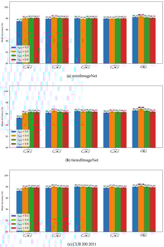
Figure 8. Mean results over 1000 episodes with bandwidth optimization for 500 iterations on cross-validations with CLIP ViT-L/14@336px feature vectors with reduced dimension $D^{\prime }$ for $r_{split}=\{0.2,0.4,0.6,0.8\}$, where $\widehat{C_{u_1}\left({\mathbf{x}}_k^{\prime }\right)}$, $\widehat{C_{u_2}\left({\mathbf{x}}_k^{\prime }\right)}$, $\widehat{C_{u_3}\left({\mathbf{x}}_k^{\prime }\right)}$, and $\widehat{C_{u_4}\left({\mathbf{x}}_k^{\prime }\right)}$ are the consensus among all iterations in the cross-validation scheme accounting for only the results of $u_1$, $u_2$, $u_3$, and $u_4$ in the consensus decision, respectively. The mean accuracy is displayed at the top of the bars for: (a) MiniImageNet. (b) TieredImageNet. (c) CUB200 2011.

Both backbones achieved a remarkable value of mean accuracy, although ViT-L/14@336px achieves the best values. It is possible to observe that, in both backbones, the consensus decision of $\widehat{C\left({\mathbf{Z}}_k\right)}$ achieved better performance than the consensus considering only one of the elements in $\mathcal{U}$. Moreover, in both backbones, the best results were achieved with $r_{split}=0.4$, implying that the consensus decision benefits from different bandwidth values that, in each iteration of the cross-validation scheme, used a considerable number of samples in ${\mathcal{V}}_i$ to optimize the bandwidth, even though the initial bandwidth value was calculated with fewer samples (${\mathcal{T}}_i$).

3.2. Five-Way One-Shot Experiments

Table 2 shows the mean results achieved for each combination of dataset and configuration of the five-way one-shot experiments using the methodology presented in Section 2.4. It is noticeable that dimensionality reduction plays an important role in our methodology, even for one-shot experiments, as the results that used a compressed version of the original dimensions $D\to D^{\prime }$ achieved consistently better results than their equivalent experiments with original dimensions.

Table 2. Mean % accuracy results alongside its 95% confidence interval results achieved for five-way one-shot image classification for miniImageNet, tieredImageNet, and CUB 200 2011 datasets. The best results achieved for each dataset are shown in bold.

		miniImageNet		tieredImageNet		CUB
CLIP Backbone	Dim. Reduction	Euclidean Distance	Cosine Similarity	Euclidean Distance	Cosine Similarity	Euclidean Distance	Cosine Similarity
ViT-B/32	No	88.73 ± 0.47	87.93 ± 0.51	84.62 ± 0.60	84.36 ± 0.61	79.85 ± 0.64	80.48 ± 0.63
ViT-B/32	Yes	88.73 ± 0.47	89.62 ± 0.46	84.62 ± 0.60	85.65 ± 0.59	79.85 ± 0.64	82.40 ± 0.58
ViT-L/14@336px	No	92.66 ± 0.39	90.39 ± 0.47	89.66 ± 0.51	87.47 ± 0.58	92.60 ± 0.45	92.16 ± 0.46
ViT-L/14@336px	Yes	92.66 ± 0.39	93.48 ± 0.36	89.66 ± 0.51	90.60 ± 0.48	92.60 ± 0.45	93.69 ± 0.40

Furthermore, cosine similarity proved to be a better choice than Euclidean distance for all the evaluated datasets, and the choice of the CLIP backbone is also important to explain the results achieved, where ViT-L/14@336px achieves a superior performance than ViT-B/32. Choosing ViT-L/14@336px instead of ViT-B/32 has such a strong effect on performance that it outweighs the combined influence of dimensionality reduction and distance metric selection.

3.3. Overall Performance

In summary, Table 3 shows the best results achieved for the datasets evaluated considering the employment of both backbones of CLIP. For the one-shot experiments, all the best results were achieved with cosine similarity and dimensionality reduction, while for the five-shot experiments, with the consensus decision group of the cross-validation ensemble, dimensionality reduction, and $r_{split}=0.4$.

Table 3. Best mean % accuracy results alongside with its 95% confidence interval achieved on five-way one-shot and five-way five-shot image classification for miniImageNet, tieredImageNet, and CUB 200 2011 datasets.

Dataset	ViT-B/32		ViT-L/14@336px
	1-Shot	5-Shot	1-Shot	5-Shot
miniImageNet	89.62 ± 0.46	96.36 ± 0.21	93.48 ± 0.36	98.37 ± 0.11
tieredImageNet	85.65 ± 0.59	93.86 ± 0.33	90.60 ± 0.48	96.84 ± 0.22
CUB	82.40 ± 0.58	93.62 ± 0.31	93.69 ± 0.40	98.16 ± 0.17

In addition to providing results with the most recurring configurations and datasets to enable the comparison of ProbaCLIP against other competitors, we also provide a more extensive evaluation of the training-free version of our method against other datasets with ViT-B/32 and ViT-L/14@336px backbones in Table 4 and Table 5, respectively.

Table 4. Performance of the training-free variant of ProbaCLIP with ViT-B/32 backbone in five-way experiments with multiple shot variations and datasets. The results show mean accuracy alongside with its 95% confidence intervals for 500 episodes.

	1-Shot	2-Shot	4-Shot	8-Shot	16-Shot
Caltech101 [44]	95.45 ± 0.50	95.18 ± 0.51	96.78 ± 0.39	98.69 ± 0.22	98.98 ± 0.22
DTD [46]	64.52 ± 0.90	62.33 ± 0.90	69.99 ± 0.81	80.97 ± 0.59	85.77 ± 0.44
FGVC-Aircraft [45]	61.51 ± 1.10	58.93 ± 1.13	65.99 ± 1.14	72.36 ± 1.06	76.65 ± 1.00
Flowers102 [42]	91.43 ± 0.67	91.42 ± 0.66	94.85 ± 0.46	98.19 ± 0.20	98.85 ± 0.15
Food101 [43]	80.30 ± 0.80	78.61 ± 0.82	85.47 ± 0.59	92.32 ± 0.35	93.76 ± 0.30

Table 5. Performance of the training-free variant of ProbaCLIP with ViT-L/14336px backbone in five-way experiments with multiple shot variations and datasets. The results show mean accuracy alongside with its 95% confidence intervals for 500 episodes.

	1-Shot	2-Shot	4-Shot	8-Shot	16-Shot
Caltech101 [44]	97.97 ± 0.34	97.40 ± 0.38	98.51 ± 0.29	99.58 ± 0.12	99.65 ± 0.17
DTD [46]	68.02 ± 0.87	65.85 ± 0.92	74.59 ± 0.83	84.48 ± 0.57	88.90 ± 0.42
FGVC-Aircraft [45]	76.99 ± 1.06	73.91 ± 1.09	79.74 ± 1.01	86.63 ± 0.85	89.10 ± 0.79
Flowers102 [42]	97.77 ± 0.33	97.08 ± 0.44	98.34 ± 0.27	99.64 ± 0.09	99.80 ± 0.04
Food101 [43]	90.09 ± 0.60	88.70 ± 0.65	93.25 ± 0.39	97.30 ± 0.20	97.90 ± 0.16

Next, we analyzed the individual contribution of each component of our method in the overall results. Table 6 presents an ablation study to support this analysis. The best performance was achieved for the cross-validation ensemble with $\mathcal{U}$ elements, dimensionality reduction, ViT-L/14@336px CLIP backbone, and bandwidth optimization. It is possible to observe that the elements that contribute more to improving performance are the choice of the CLIP backbone, the ensemble decision, and dimensionality reduction.

Table 6. Ablation studies of the methodology proposed for five-way five-shot experiments, where the best accuracy among all the $r_{split}$ values tested for each of the configurations is displayed. The setup that achieved the best results and its results are shown in bold.

Setup	miniImageNet	tieredImageNet	CUB
ViT-B/32 with D for $u_1$ setup	95.26 ± 0.23	92.21 ± 0.38	91.03 ± 0.39
+ h optimization	95.34 ± 0.23	92.38 ± 0.37	91.45 ± 0.36
+ Dim. reduction (PCA)	95.57 ± 0.22	92.62 ± 0.37	91.82 ± 0.36
+ Change to ViT-L/14@336px	97.80 ± 0.15	95.88 ± 0.26	97.61 ± 0.20
+ cross-validation ($u_1$)	98.07 ± 0.14	96.33 ± 0.24	97.89 ± 0.19
+ Ensemble with $\mathcal{U}$ elements	98.37 ± 0.11	96.84 ± 0.22	98.16 ± 0.17
−h optimization (100% training-free)	98.17 ± 0.15	96.72 ± 0.23	97.91 ± 0.20

Although the best performance was achieved with bandwidth optimization, the result of a fully training-free option achieves a very similar performance, so that, for all datasets, it intersects with the best results considering the confidence intervals.

3.4. Impact of the Dimensionality on the Performance

A more detailed study of the impact of the number of dimensions in the dimensionality reduction was conducted to provide a deeper understanding of its role in the presented methodology. For that, a new experiment was sketched, varying the number of shots N within the set $\{5,10,20\}$ with original and reduced dimensions, where, for each value of N, the targeted dimensions of PCA were forced to 25%, 50%, 75%, and 100% of the maximum number of components allowed. It is important to recall that due to the rank constraint of the data matrix in PCA, the number of principal components that can be meaningfully extracted from a dataset $X\in {\mathbb{R}}^{n\times d}$ is bounded by $min(n,d)$, which in this case is $min(M\times N\times r_{split},D)$. The experiments were carried out with the training-free version of ProbaCLIP and repeated for 500 episodes for each combination. The results are presented in Figure 9.

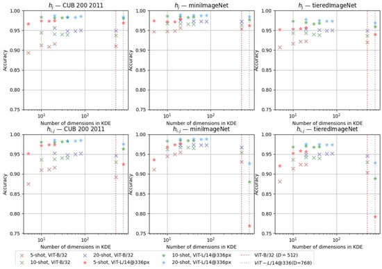
Figure 9. Impact of the number of samples per class (N-shot) and the number of dimensions in the KDE on the classification accuracy, considering a unique KDE per dataset. The results were plotted for CUB 200 2011, miniImageNet, and tieredImageNet with ViT-B/32 and ViT-L/14@336 backbones.

It is noticeable from the plots that the more shots, the higher the accuracy tends to be. In other words, the more examples the classifier has per class, the better the expected performance. In addition, the higher the percentage of $PCs$ within $P{C}_{opt}$, the better the results tend to be as well, reinforcing the choice of using the principal components that explain 99% of the variance.

3.5. Qualitative Analysis

To improve the understanding of the performance achieved by our method, we also provide a qualitative analysis with the CUB200 2011 dataset. Two experiments were executed, namely A and B, where experiment A uses a varied set of classes for five-way five-shot experiments, while the classes in experiment B were artificially chosen to have a subset of very similar classes together with dissimilar classes. Experiments A and B were conducted with CUB200 2011 and are shown in Figure 10 and Figure 11, respectively.

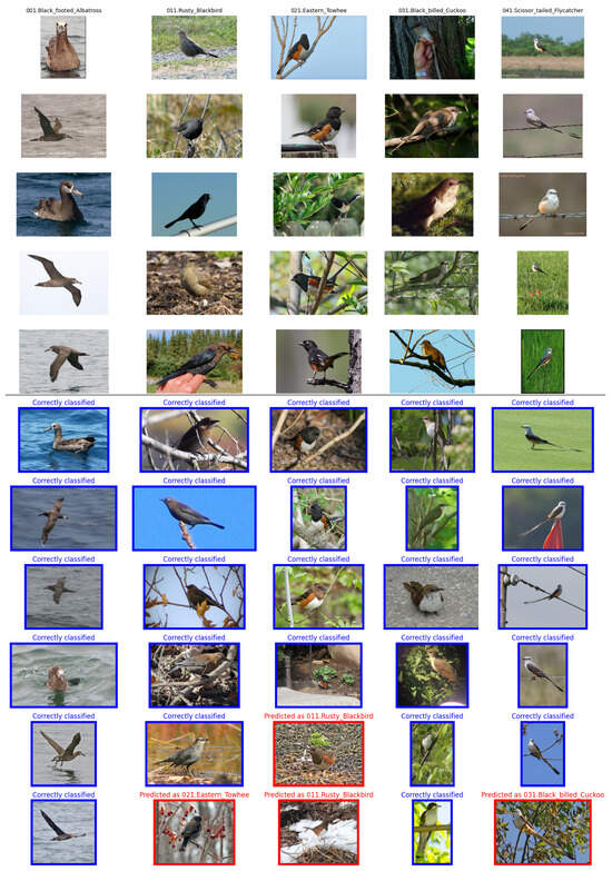
Figure 10. Result of the qualitative experiment A: representation of a common random class assignation to the five-way five-shot paradigm with CUB200 2011 dataset, where each image column represents one of the five image classes with its name written on the top. The images above the horizontal black line are those belonging to $\mathcal{S}$, while the ones below are a subset of $\mathcal{Q}$ that shows a few correct and wrong (if they exist) predictions per class. The accuracy recorded for the ensemble of classifiers in this episode was 98.91%. Images with blue contours were predicted correctly, while those with red contours were not.

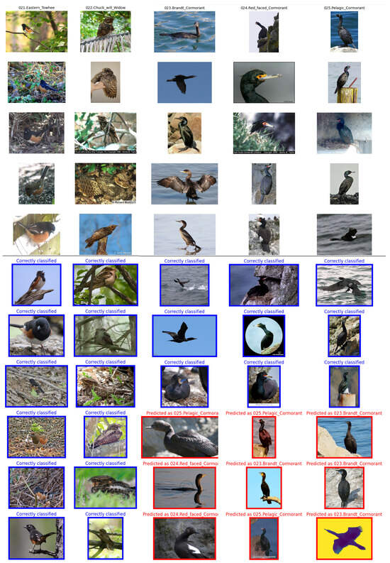
Figure 11. Result of the qualitative experiment B: representation of a more rare random class assignation to the five-way five-shot paradigm with CUB200 2011 dataset, where three of the classes are very similar to each other while the other two are visually more dissimilar. Each image column represents one of the five image classes with its name written on the top. The images above the horizontal black line are those belonging to $\mathcal{S}$, while the ones below are a subset of $\mathcal{Q}$ that shows a few correct and wrong (if they exist) predictions per class. The accuracy recorded for the ensemble of classifiers in this episode was 80.53%. Images with blue contours were predicted correctly, while those with red contours were not.

In experiment A, only four images were misclassified (shown with a red border) by our ensemble of classifiers, and the classification accuracy was 98.91%. In this case, our method was very efficient in predicting the correct class of the vast majority of images. One possible explanation for the two images belonging to the class 021.Eastern_Towhee and predicted as 011.Rusty_Blackbird is that they are standing on the ground. Observing the training images, it is possible to notice that the only class with several samples of birds standing on the ground is 011.Rusty_Blackbird. Furthermore, looking at the random selection of samples in $\mathcal{S}$ for 011.Rusty_Blackbird, it is noticeable that they are quite different from each other, which, in this case, might have influenced the model to focus on the similarity between images rather than the type of birds for these misclassified examples.

We compared an episode with average performance with another more rare episode that achieved worse performance by our classifier. Thus, in experiment B, three types of cormorants, which are quite similar to each other, were intentionally put together with two different species of birds. In this case, the classification accuracy was significantly lower (80.53%). Although all images in $\mathcal{Q}$ belong to 021.Eastern_Towhee and 022.Chuck_will_Widow were correctly classified, there were some images belonging to the cormorant classes that were incorrectly assigned to other cormorant classes. In other words, the dissimilarity between the classes 021.Eastern_Towhee and 022.Chuck_will_Widow is quite evident, which facilitated the PCA and KDE to concentrate on them. However, the difference between the cormorant classes is milder, which made the classifier’s task in these classes more difficult. This artificial example shows that episodes having both very similar and dissimilar classes can be more challenging.

Nevertheless, imagining that the classification would be carried out manually by a human, and observing the images in $\mathcal{S}$ and $\mathcal{Q}$ for the cormorant classes, it would be quite challenging to correctly classify some of the images.

3.6. Computational Impact of the Bandwidth Optimization

We also provide an analysis of our strategy in terms of its computational effort to show how lightweight our method is. Table 7 compares the average time required to extract the CLIP embeddings and to run ProbaCLIP with and without the bandwidth optimization process. It can be observed that the training-free ProbaCLIP takes two orders of magnitude less time to execute than the feature extraction process. Thus, if the downstream application in which ProbaCLIP is used requires low inference time, the training-free approach with a simpler backbone, such as ViT-B/32, is the best choice. On the other hand, the few-shot episodes with ProbaCLIP and bandwidth optimization take significantly longer, although they are of a similar order of magnitude to the feature extraction task.

Table 7. Time duration of ProbaCLIP classification episode averaged over ten episodes considering 100 images evenly split in five classes executing five-way five-shot classification, where 25 images are assigned to $\mathcal{S}$ and 75 to $\mathcal{Q}$. The experiment was conducted with a notebook Asus TUF-Gaming-A15 with an AMD Ryzen™ 9 7940HS processor and a GeForce RTX 4070 Laptop GPU.

Task	Avg. Time [seconds]
	ViT-B/32	ViT-L/14@336px
CLIP feature extraction	9.57	24.56
Training-free ProbaCLIP prediction	0.10	0.10
ProbaCLIP prediction with h optimization	42.73	63.35

3.7. Comparison with the State-of-the-Art Methods

Table 8 benchmarks our approach against three recent surveys, situating it within a broader landscape of competitive few-shot classifiers evaluated under standard five-way one-shot and five-shot protocols on miniImageNet, tieredImageNet, and CUB200 2011. In the first comprehensive review, Li et al. [47] provide a taxonomy of deep metric learning methods for few-shot classification, organized into three stages: feature embedding, class representation, and distance measurement. Their survey analyzes more than 60 methods published between 2018 and 2022. Although our method does not strictly belong to the deep metric learning paradigm, we compare against this body of work because it represents the category most closely aligned with our approach. Both deep metric learning and our KDE-based framework rely on a shared principle: classification is performed in a learned embedding space by comparing similarity relationships rather than by training task-specific classifiers. Within this design space, our method advances the state of the art by combining frozen CLIP embeddings with statistically principled density estimation, yielding superior performance and enhanced interpretability.

Table 8. The comparison of the best results achieved by ProbaCLIP against survey papers. The best results achieved for each dataset and experiment are shown in bold.

	miniImageNet		tieredImageNet		CUB
Method	1-Shot	5-Shot	1-Shot	5-Shot	1-Shot	5-Shot
Best result [47]	82.16	89.80	–	–	67.90 ± 0.90	85.39 ± 0.56
Qty. of methods assessed in [47]	37	40	–	–	8	8
Best result [48]	84.32 ± 0.21	90.02 ± 0.12	89.65 ± 0.22	93.21 ± 0.13	91.69 ± 0.18	95.02 ± 0.16
Qty. of methods assessed in [48]	97	97	75	75	34	34
Best result [49]	–	–	–	–	65.05 ± 0.83	84.21 ± 0.18
Qty. of methods assessed in [49]	–	–	–	–	12	15
Training-free ProbaCLIP	3.48 ± 036	98.17 ± 0.15	90.60 ± 0.48	96.72 ± 0.23	93.69 ± 0.40	97.91 ± 0.20
ProbaCLIP w/h optimization	-	98.77 ± 0.11	-	96.84 ± 0.22	-	98.16 ± 0.17

In the second survey, Yang et al. [48] provided a broader umbrella review of generalized few-shot learning, integrating zero-shot, few-shot, and generalized zero-shot tasks under a unified theoretical framework. Their best-in-review results remain significantly below our performance, reinforcing the novelty and efficacy of KDE-based density estimation in the CLIP feature space with information condensed in a lower-dimensional space.

In the last survey, Xu et al. [49] provided results of few-shot image classification trained in cross-domain. The paper displayed the performance of numerous deep learning approaches on datasets that differ from the ones they were trained. Although no foundational models such as CLIP were mentioned in this survey, the comparison is also pertinent as we extract feature vectors from a neural network trained on a dataset that differs from the datasets that we test.

Then, we further compared our approach with other recent publications, not included in these surveys, that used the CLIP embeddings for few-shot learning and achieved state-of-the-art results. Table 9 shows this comparison, where our approach achieves the best performance for tieredImageNet and competitive performance for miniImageNet.

SgVA-CLIP [23] fine tunes a visual adapter on base classes with cross-modal distillation, achieving remarkable performance on miniImageNet and tieredImageNet. By contrast, our method keeps CLIP frozen and does not require gradient-based training. Although our method proposes an optimization process for bandwidth selection, this process is a low-dimensional and much simpler optimization, unlike the large-scale backpropagation needed for adapter training. Despite its simplicity, our ViT-L/14@336 results are competitive (miniImageNet) or superior (tieredImageNet), while incurring far less compute and training overhead.

Ferragu et al. [8] propose Multi-modal CLIP Inference (MM-CLIP), a training-free baseline ensembling CLIP’s visual and textual scores. With ViT-L/14, they report state-of-the-art results with miniImageNet and show strong results on other datasets as well. Our method shares the training-free deployment philosophy but differs in two key ways: (i) it is prompt-free, avoiding prompt engineering; and (ii) it is probabilistic, producing per-class likelihoods using KDE rather than combining scores. While MM-CLIP edges us in miniImageNet using textual embeddings, our pipeline is simpler because it only uses visual embeddings, is less sensitive to prompt calibration, and significantly outperforms the variant of MM-CLIP that uses only visual embeddings. Furthermore, our method models class-conditional distributions in the embedding space with KDE, providing likelihoods that naturally reflect the confidence of each prediction. This enables principled uncertainty estimation, in contrast to methods such as MM-CLIP, which rely on heuristic score-level ensembling.

In addition, Simple Semantic-Aided FSL (SemFew) [50] improves high-quality textual descriptions and then feeds both the paraphrased semantics and visual features into a two-layer Semantic Alignment Network to construct robust class prototypes, avoiding intricate multi-modal fusion while relying on richer semantics than bare class names. In another direction, FEL-FRN [51] augments a feature map reconstruction pipeline with efficient channel attention and fuses its scores with a Long-CLIP branch; classification is driven by per-location reconstruction of query feature maps from support features, while Long-CLIP provides text-guided few-shot cues that are combined using learned weights, particularly benefiting fine-grained categories with multiple attribute variation. Finally, PrototypeFormer [52] instead learns class prototypes with a lightweight transformer prototype extraction module over CLIP image embeddings and strengthens them by a prototype contrastive loss computed on leave-one-out sub-prototypes, then queries are classified by distance to the refined prototypes. Different from these methods, ProbaCLIP does not depend on textual information or additional training, and it still outperforms them (or is equivalent for FEL-FRN in CUB, which has overlapping confidence intervals).

Table 9. The comparison of the best results achieved against episodic methodologies that use the CLIP embeddings for five-way five-shot image classification. The results intersecting the confidence intervals of the best results achieved for each dataset are shown in bold.

Method	miniImageNet	tieredImageNet	CUB
SgVA-CLIP [23]	98.72 ± 0.13	96.21 ± 0.37	–
MM-CLIP (visual embedding) [8]	96.65 ± 0.06	–	–
MM-CLIP (textual embedding) [8]	99.38 ± 0.02	–	–
MM-CLIP (stacked-avg) [8]	98.88 ± 0.09	–	–
SemFew-Trans [50]	86.49 ± 0.50	89.89 ± 0.52	–
PrototypeFormer [52]	97.07 ± 0.11	95.00 ± 0.19	94.25 ± 0.16
FEL-FRN [51]	–	–	97.68 ± 0.59
Training-free ProbaCLIP (ours)	98.17 ± 0.15	96.72 ± 0.23	97.91 ± 0.20
ProbaCLIP w/h optimization (ours)	98.37 ± 0.11	96.84 ± 0.22	98.16 ± 0.17

Table 9. The comparison of the best results achieved against episodic methodologies that use the CLIP embeddings for five-way five-shot image classification. The results intersecting the confidence intervals of the best results achieved for each dataset are shown in bold.

Method	miniImageNet	tieredImageNet	CUB
SgVA-CLIP [23]	98.72 ± 0.13	96.21 ± 0.37	–
MM-CLIP (visual embedding) [8]	96.65 ± 0.06	–	–
MM-CLIP (textual embedding) [8]	99.38 ± 0.02	–	–
MM-CLIP (stacked-avg) [8]	98.88 ± 0.09	–	–
SemFew-Trans [50]	86.49 ± 0.50	89.89 ± 0.52	–
PrototypeFormer [52]	97.07 ± 0.11	95.00 ± 0.19	94.25 ± 0.16
FEL-FRN [51]	–	–	97.68 ± 0.59
Training-free ProbaCLIP (ours)	98.17 ± 0.15	96.72 ± 0.23	97.91 ± 0.20
ProbaCLIP w/h optimization (ours)	98.37 ± 0.11	96.84 ± 0.22	98.16 ± 0.17

3.8. Potential Challenges, Limitations and Future Work

Despite the advantages that ProbaCLIP provides, in scenarios where the class distributions in the CLIP embedding space are highly overlapping or very fine-grained, the KDE-based classification may experience degraded performance. Specifically, if some of the classes in a given episode produce very similar embeddings, as observed in Figure 11, it could make a density-based classifier without additional adaptation struggle to distinguish them. This limitation, although mitigated by compressing the most relevant dissimilarities between classes into a few dimensions with PCA, is partly a consequence of using a fixed feature extractor, as it cannot explicitly learn new discriminative features for confusing classes. In this context, simple solutions such as the careful selection of classes in each episode or the choice of other types of kernels to handle density estimation could be evaluated. Or more sophisticated ones, such as the employment of more specialized loss techniques to reduce inter-class mutual feature information, like the one introduced by DCLIP [32], could be explored in future works.

Moreover, reliance on a pre-trained model such as CLIP means that the method inherits its biases or blind spots, and its deployment must consider the memory and compute requirements of the CLIP backbone for inference. These factors highlight the importance of knowing the downstream task before applying the method in practice.

In another direction, it has been shown that CLIP ViT-based models may face challenges to interpret images under certain visual conditions, particularly when objects are partially occluded, viewed from atypical poses, or subject to geometric distortions and 3D corruptions such as motion blur or viewpoint shifts [53]. Although these issues have not been addressed in the present work, we recognize that future efforts could strengthen the robustness of the presented methodology under such conditions. Recent studies on robust feature representations in human parsing have shown that domain transforms such as polar harmonic Fourier moments and boundary-guided consistency can significantly improve stability in complex scenes [54]. Toward the same direction, the use of quaternion polar harmonic Fourier moments is shown to be effective in dealing with geometrically distorted light-field RGB images [55]. These works could inspire a more robust handling of geometrically distorted environments.

Looking ahead, there are other promising directions to further enhance and extend our approach. An interesting possibility is to benefit from multi-modal information. Since CLIP is a vision-language model, one could study how to extract relevant information from its textual branch or to incorporate additional textual information from class names or descriptions without requiring additional textual information during inference. Then, combining cues from both modalities to improve accuracy. Such an extension might retain our training-free ethos by leveraging CLIP’s text encoder for zero-shot guidance or refining the image densities with semantic priors, as evidenced by recent multi-modal CLIP inference methods. Another important direction is online adaptation and continual learning. Our current method works in a batch few-shot setting; enabling it to update the density models incrementally as new data arrives or classes emerge (without retraining from scratch) would make it robust in non-stationary environments. Techniques from online or task-agnostic meta learning could be borrowed to allow the KDE to adjust to evolving feature distributions while avoiding catastrophic forgetting. Additionally, further exploration of the uncertainty estimation capabilities of our probabilistic approach would be another interesting path. Since our classifier produces a likelihood for each class, we naturally obtain confidence measures for predictions; future work can utilize these likelihoods for calibrating predictions, detecting out-of-distribution queries, or flagging highly uncertain cases for human review. Finally, to facilitate real-time deployment in simpler hardware, one could investigate model compression or distillation techniques for the CLIP backbone to reduce latency and memory usage. By listing these possible improvements, we aim to broaden the applicability of training-free few-shot classification and ensure that our KDE-based classifier remains at the forefront of practical and reliable few-shot recognition across diverse domains.

4. Conclusions

In this work, we introduced ProbaCLIP, a training-free few-shot image classification approach that leverages CLIP’s powerful embeddings in a kernel density estimation framework. By modeling each new class’ feature distribution with KDE and classifying queries using likelihood evaluation in the embedding space, our method does not require gradient-based fine-tuning, prompt engineering, auxiliary meta learning phases, or additional training schemes. We demonstrated that compressing relevant information within the context of each episode by reducing the dimensionality of the CLIP embeddings with the principal component analysis is highly beneficial, significantly increasing the ability to differentiate between classes. Furthermore, we proposed an optional optimization scheme to find the bandwidth values for each episode that maximizes classification accuracy, which was able to further increase the performance by adding a tiny gradient search with very few parameters (at maximum one parameter per class) trained only on the few samples of each episode’s support set. However, although this optimization scheme usually contributes to slightly improved results, we demonstrated that the training-free approach—without bandwidth optimization—can also compete with the state-of-the-art methods, achieving consistently better or equivalent results than its competitors in standard few-shot benchmarks. The mean accuracy over 1000 episodes achieved by the training-free ProbaCLIP for miniImageNet, tieredImageNet, and CUB-200-2011 in a five-way five-shot framework are, respectively, 98.17 ± 0.15, 96.72 ± 0.23, and 97.91 ± 0.20, while the mean accuracy on the same datasets with a bandwidth optimization is 98.37 ± 0.11, 96.84 ± 0.22, and 98.16 ± 0.17. The results establish that a simple, prompt-free probabilistic inference on high-quality pre-trained features can match or exceed more complex pipelines that require training or prompt information, significantly reducing computational complexity.

A key strength of our method is its scalability and efficiency, which make it especially appealing for low-data, compute-constrained settings. Since no additional training is required to adapt to new classes, the method can scale to many tasks or classes with minimal overhead. This property is highly valuable in real-world scenarios where collecting large labeled datasets or performing extensive fine-tuning is impractical. Moreover, the compact inference pipeline is well-suited for edge deployment, where the absence of heavy training means models can be deployed on resource-limited devices without cloud computing dependency, facilitating real-time or on-device operation, and broadening their applicability to embedded and time-critical systems.

References

- Pachetti, E.; Colantonio, S. A systematic review of few-shot learning in medical imaging. Artif. Intell. Med. 2024, 156, 102949. [Google Scholar] [CrossRef]
- Liu, J.; Fan, K.; Cai, X.; Niranjan, M. Few-shot learning for inference in medical imaging with subspace feature representations. PLoS ONE 2024, 19, e0309368. [Google Scholar] [CrossRef]
- Zhang, Y.; Liu, C. Few-shot crack image classification using clip based on bayesian optimization. arXiv 2025, arXiv:2503.00376. [Google Scholar] [CrossRef]
- Zajec, P.; Rožanec, J.M.; Theodoropoulos, S.; Fontul, M.; Koehorst, E.; Fortuna, B.; Mladenić, D. Few-shot learning for defect detection in manufacturing. Int. J. Prod. Res. 2024, 62, 6979–6998. [Google Scholar] [CrossRef]
- García-Díaz, J.A.; Pan, R.; Valencia-García, R. Leveraging Zero and Few-Shot Learning for Enhanced Model Generality in Hate Speech Detection in Spanish and English. Mathematics 2023, 11, 5004. [Google Scholar] [CrossRef]
- Halitaj, A.; Zubiaga, A. ALPET: Active few-shot learning for citation worthiness detection in low-resource Wikipedia languages. Expert Syst. Appl. 2025, 281, 127503. [Google Scholar] [CrossRef]
- Tian, S.; Li, L.; Li, W.; Ran, H.; Ning, X.; Tiwari, P. A survey on few-shot class-incremental learning. Neural Netw. 2024, 169, 307–324. [Google Scholar] [CrossRef] [PubMed]
- Ferragu, C.; Chagniot, P.; Coyette, V. Multimodal CLIP Inference for Meta-Few-Shot Image Classification. arXiv 2024, arXiv:2405.10954. [Google Scholar]
- Anjum, U.; Stockman, C.; Luong, C.; Zhan, J. Domain-Generalization to Improve Learning in Meta-Learning Algorithms. arXiv 2025, arXiv:2508.09418. [Google Scholar]
- Sow, D.; Lin, S.; Liang, Y.; Zhang, J. Task-Agnostic Online Meta-Learning in Non-Stationary Environments. 2023. Available online: https://openreview.net/forum?id=jsZ8PDQOVU (accessed on 6 November 2025).
- Ma, H.; Fan, B.; Ng, B.K.; Lam, C.T. CLG: Contrastive Label Generation with Knowledge for Few-Shot Learning. Mathematics 2024, 12, 472. [Google Scholar] [CrossRef]
- Radford, A.; Kim, J.W.; Hallacy, C.; Ramesh, A.; Goh, G.; Agarwal, S.; Sastry, G.; Askell, A.; Mishkin, P.; Clark, J.; et al. Learning transferable visual models from natural language supervision. In Proceedings of the International Conference on Machine Learning, PmLR, Virtual Event, 18–24 July 2021; pp. 8748–8763. [Google Scholar]
- Jia, C.; Yang, Y.; Xia, Y.; Chen, Y.T.; Parekh, Z.; Pham, H.; Le, Q.; Sung, Y.H.; Li, Z.; Duerig, T. Scaling up visual and vision-language representation learning with noisy text supervision. In Proceedings of the International Conference on Machine Learning, PMLR, Virtual Event, 18–24 July 2021; pp. 4904–4916. [Google Scholar]
- Singh, A.; Hu, R.; Goswami, V.; Couairon, G.; Galuba, W.; Rohrbach, M.; Kiela, D. Flava: A foundational language and vision alignment model. In Proceedings of the IEEE/CVF Conference on Computer Vision and Pattern Recognition, New Orleans, LA, USA, 18–24 June 2022; pp. 15638–15650. [Google Scholar]
- Zhai, X.; Mustafa, B.; Kolesnikov, A.; Beyer, L. Sigmoid loss for language image pre-training. In Proceedings of the IEEE/CVF International Conference on Computer Vision, Paris, France, 4–6 October 2023; pp. 11975–11986. [Google Scholar]
- Li, Z.; Wu, X.; Du, H.; Liu, F.; Nghiem, H.; Shi, G. A Survey of State of the Art Large Vision Language Models: Benchmark Evaluations and Challenges. In Proceedings of the Computer Vision and Pattern Recognition Conference, Nashville, TN, USA, 11–17 June 2025; pp. 1587–1606. [Google Scholar]
- Liu, H.; Li, C.; Wu, Q.; Lee, Y.J. Visual instruction tuning. Adv. Neural Inf. Process. Syst. 2023, 36, 34892–34916. [Google Scholar]
- Wang, P.; Bai, S.; Tan, S.; Wang, S.; Fan, Z.; Bai, J.; Chen, K.; Liu, X.; Wang, J.; Ge, W.; et al. Qwen2-vl: Enhancing vision-language model’s perception of the world at any resolution. arXiv 2024, arXiv:2409.12191. [Google Scholar]
- Dai, W.; Lee, N.; Wang, B.; Yang, Z.; Liu, Z.; Barker, J.; Rintamaki, T.; Shoeybi, M.; Catanzaro, B.; Ping, W. Nvlm: Open frontier-class multimodal llms. arXiv 2024, arXiv:2409.11402. [Google Scholar] [CrossRef]
- Jayasumana, S.; Ramalingam, S.; Veit, A.; Glasner, D.; Chakrabarti, A.; Kumar, S. Rethinking fid: Towards a better evaluation metric for image generation. In Proceedings of the IEEE/CVF Conference on Computer Vision and Pattern Recognition, Seattle, WA, USA, 16–22 June 2024; pp. 9307–9315. [Google Scholar]
- Xiao, C.; Chung, I.; Kerboua, I.; Stirling, J.; Zhang, X.; Kardos, M.; Solomatin, R.; Moubayed, N.A.; Enevoldsen, K.; Muennighoff, N. MIEB: Massive image embedding benchmark. arXiv 2025, arXiv:2504.10471. [Google Scholar] [CrossRef]
- Kato, N.; Nota, Y.; Aoki, Y. Proto-Adapter: Efficient Training-Free CLIP-Adapter for Few-Shot Image Classification. Sensors 2024, 24, 3624. [Google Scholar] [CrossRef]
- Peng, F.; Yang, X.; Xiao, L.; Wang, Y.; Xu, C. Sgva-clip: Semantic-guided visual adapting of vision-language models for few-shot image classification. IEEE Trans. Multimed. 2023, 26, 3469–3480. [Google Scholar] [CrossRef]
- Sun, T.; Yang, H.; Li, Z.; Xu, X.; Wang, X. Adversarial domain adaptation with CLIP for few-shot image classification. Appl. Intell. 2025, 55, 59. [Google Scholar] [CrossRef]
- Chen, J.; Yuan, H.; Xie, B. MIF: Multi-source information fusion for few-shot classification with CLIP. Pattern Recognit. Lett. 2025, 192, 113–121. [Google Scholar] [CrossRef]
- Martin, S.; Huang, Y.; Shakeri, F.; Pesquet, J.C.; Ben Ayed, I. Transductive zero-shot and few-shot clip. In Proceedings of the IEEE/CVF Conference on Computer Vision and Pattern Recognition, Seattle, WA, USA, 16–22 June 2024; pp. 28816–28826. [Google Scholar]
- Hughes, G.F. On the mean accuracy of statistical pattern recognizers. IEEE Trans. Inf. Theory 1968, 14, 55–63. [Google Scholar] [CrossRef]
- Donoho, D.L. High-dimensional data analysis: The curses and blessings of dimensionality. In Proceedings of the AMS Conference Math Challenges 21st Century, Los Angeles, CA, USA, 6–11 August 2000; Available online: https://sunju.org/teach/TMML-Fall-2021/Donoho-2000.pdf (accessed on 6 November 2025).
- Duda, R.O.; Hart, P.E.; Stork, D.G. Pattern Classification, 2nd ed.; Wiley-Interscience: Hoboken, NJ, USA, 2000. [Google Scholar]
- Jolliffe, I.T.; Cadima, J. Principal component analysis: A review and recent developments. Philos. Trans. R. Soc. A Math. Phys. Eng. Sci. 2016, 374, 20150202. [Google Scholar] [CrossRef]
- Rassoul, A.; Belguerna, A.; Daoudi, H.; Elmezouar, Z.C.; Alshahrani, F. On the Exact Asymptotic Error of the Kernel Estimator of the Conditional Hazard Function for Quasi-Associated Functional Variables. Mathematics 2025, 13, 2172. [Google Scholar] [CrossRef]
- Rawlekar, S.; Cai, Y.; Wang, Y.; Yang, M.H.; Ahuja, N. Efficiently Disentangling CLIP for Multi-Object Perception. arXiv 2025, arXiv:2502.02977. [Google Scholar]
- Silverman, B.W. Density Estimation for Statistics and Data Analysis; Chapman and Hall/CRC: London, UK, 1986. [Google Scholar]
- Scott, D.W. Multivariate Density Estimation: Theory, Practice, and Visualization; John Wiley & Sons: New York, NY, USA, 1992. [Google Scholar]
- García Portugués, E. Notes for Predictive Modeling. 2025. Available online: https://bookdown.org/egarpor/PM-UC3M/ (accessed on 6 November 2025).
- Wand, M.P.; Jones, M.C. Kernel Smoothing; CRC Press: Boca Raton, FL, USA, 1994. [Google Scholar]
- Kingma, D.P.; Ba, J. Adam: A method for stochastic optimization. arXiv 2014, arXiv:1412.6980. [Google Scholar]
- Ashok, A.; miniImageNet Dataset. Pre-Processed Version. Available online: https://www.kaggle.com/datasets/arjunashok33/miniimagenet (accessed on 25 August 2025).
- Vinyals, O.; Blundell, C.; Lillicrap, T.; Kavukcuoglu, K.; Wierstra, D. Matching Networks for One Shot Learning. In Proceedings of the 30th International Conference on Neural Information Processing Systems (NeurIPS), Barcelona, Spain, 5–10 December 2016; pp. 3637–3645. [Google Scholar]
- Ren, M.; Triantafillou, E.; Ravi, S.; Snell, J.; Swersky, K.; Tenenbaum, J.; Larochelle, H.; Zemel, R. Meta-Learning for Semi-Supervised Few-Shot Classification. In Proceedings of the 6th International Conference on Learning Representations (ICLR), Vancouver, BC, Canada, 30 April–3 May 2018. [Google Scholar]
- Wah, C.; Branson, S.; Welinder, P.; Perona, P.; Belongie, S. The Caltech-UCSD Birds-200-2011 Dataset; Technical Report; California Institute of Technology: Pasadena, CA, USA, 2011. [Google Scholar]
- Nilsback, M.E.; Zisserman, A. Automated flower classification over a large number of classes. In Proceedings of the 2008 Sixth Indian Conference on Computer Vision, Graphics & Image Processing, Bhubaneswar, India, 16–19 December 2008; pp. 722–729. [Google Scholar]
- Bossard, L.; Guillaumin, M.; Van Gool, L. Food-101–mining discriminative components with random forests. In Proceedings of the European Conference on Computer Vision, Zurich, Switzerland, 6–12 September 2014; Springer: Zurich, Switzerland, 2014; pp. 446–461. [Google Scholar]
- Fei-Fei, L.; Fergus, R.; Perona, P. One-shot learning of object categories. IEEE Trans. Pattern Anal. Mach. Intell. 2006, 28, 594–611. [Google Scholar] [CrossRef]
- Maji, S.; Rahtu, E.; Kannala, J.; Blaschko, M.; Vedaldi, A. Fine-grained visual classification of aircraft. arXiv 2013, arXiv:1306.5151. [Google Scholar] [CrossRef]
- Cimpoi, M.; Maji, S.; Kokkinos, I.; Mohamed, S.; Vedaldi, A. Describing textures in the wild. In Proceedings of the IEEE Conference on Computer Vision and Pattern Recognition, Columbus, OH, USA, 23–28 June 2014; pp. 3606–3613. [Google Scholar]
- Li, X.; Yang, X.; Ma, Z.; Xue, J.H. Deep metric learning for few-shot image classification: A Review of recent developments. Pattern Recognit. 2023, 138, 109381. [Google Scholar] [CrossRef]
- Yang, S.; Hu, B.; Liu, F.; Wu, X.; Ding, W.; Zhou, J. A Comprehensive Review for Generalized Few-Shot Imageclassification. 2024. Available online: https://ssrn.com/abstract=5080987 (accessed on 25 August 2025).
- Xu, H.; Zhi, S.; Sun, S.; Patel, V.; Liu, L. Deep learning for cross-domain few-shot visual recognition: A survey. ACM Comput. Surv. 2025, 57, 1–37. [Google Scholar] [CrossRef]
- Zhang, H.; Xu, J.; Jiang, S.; He, Z. Simple semantic-aided few-shot learning. In Proceedings of the IEEE/CVF Conference on Computer Vision and Pattern Recognition, Seattle, WA, USA, 17–21 June 2024; pp. 28588–28597. [Google Scholar]
- Wang, Y.; Zhang, A.; Liu, J.; Wu, K.; Abdullahi, H.S.; Lv, P.; Gao, Y.; Zhang, H. FEL-FRN: Fusion ECA long-CLIP feature reconstruction network for few-shot classification. J. Big Data 2025, 12, 104. [Google Scholar] [CrossRef]
- Su, M.; He, F.; Li, G.; Li, F. PrototypeFormer: Learning to explore prototype relationships for few-shot image classification. Neurocomputing 2025, 640, 130326. [Google Scholar] [CrossRef]
- Tu, W.; Deng, W.; Gedeon, T. Toward a Holistic Evaluation of Robustness in CLIP Models. IEEE Trans. Pattern Anal. Mach. Intell. 2025, 47, 8280–8296. [Google Scholar] [CrossRef]
- Liu, Y.; Wang, C.; Lu, M.; Yang, J.; Gui, J.; Zhang, S. From simple to complex scenes: Learning robust feature representations for accurate human parsing. IEEE Trans. Pattern Anal. Mach. Intell. 2024, 46, 5449–5462. [Google Scholar] [CrossRef] [PubMed]
- Wang, C.; Zhang, Q.; Wang, X.; Zhou, L.; Li, Q.; Xia, Z.; Ma, B.; Shi, Y.Q. Light-Field Image Multiple Reversible Robust Watermarking Against Geometric Attacks. IEEE Trans. Dependable Secur. Comput. 2025. [Google Scholar] [CrossRef]
Disclaimer/Publisher’s Note: The statements, opinions and data contained in all publications are solely those of the individual author(s) and contributor(s) and not of MDPI and/or the editor(s). MDPI and/or the editor(s) disclaim responsibility for any injury to people or property resulting from any ideas, methods, instructions or products referred to in the content. |
© 2025 by the authors. Licensee MDPI, Basel, Switzerland. This article is an open access article distributed under the terms and conditions of the Creative Commons Attribution (CC BY) license (https://creativecommons.org/licenses/by/4.0/).