An Efficient Improved Constrained Greedy Optimization Algorithm for Phase Load Balancing in Low-Voltage Distribution Networks

Abstract

With regard to low-voltage (LV) distribution networks, the quality of distributed electricity can be compromised by the level of phase load imbalance. Consequently, numerous phase load balancing (PLB) algorithms have been proposed in the specialized literature. However, those models have been focused on the quality of the solution obtained rather than performance, which leads to reduced practical applicability for the distribution network (reduced scalability, slow convergence, and a higher computational cost). Furthermore, certain constraints regarding the electrical network and the switching operations of consumers must be integrated into the mathematical model. In this context, the proposed PLB algorithm represents an improved constrained greedy optimization (ICGO), capable of achieving fast convergence even on large datasets, with a lower computational cost. Three scenarios (30, 250, and 500 consumers), each with 20 distinct initial non-symmetries, were simulated. The results support the practical effectiveness and scalability of the ICGO: an absolute value of the neutral current below 0.63 A (99.53% relatively reduction), a current unbalance index below 0.1%, a small number of iterations (between 4 and 11 iterations), and an execution time between 0.00051 and 0.01149 s). Therefore, this research proposes an efficient PLB algorithm, with the possibility for its improvement in future work.

1. Introduction

The well-known but constantly topical problems regarding electricity systems relate to the quality and continuity of the electricity supply. The asymmetrical operating mode of an LV distribution network causes a series of technical problems such as power losses, additional thermal stresses on electrical conductors, network instability, and disruptive effects on other networks [1,2,3,4,5,6,7,8,9,10]. A considerable amount of research has been devoted to the numerical simulation of PLB, implicitly the process management algorithm [11]. However, of great importance for the PLB process is the design of a flexible, simple, robust, and efficient algorithm that can be applied in distribution networks and that can respond to technical constraints.

In power systems, the three-phase distribution network is not found in the ideal mathematical representation of a symmetrical network—a three-phase system of sinusoidal quantities (voltage/current) characterized by the three phasors equal in modulus and successively out of phase, one with respect to the other, with an angle equal to 2π/3 [1,3,5,6]. Even less so in LV networks, where the distribution of loads is unequal in the three phases. Also, considering that the behavior of consumers in the network is characterized by a dynamism specific to their operation, the mentioned symmetry remains only theoretical. The causes that determine the appearance of the non-symmetric regime can be divided into two large categories [3]:

• Causes related to temporary non-symmetry;
• Causes related to permanent non-symmetry.

The temporary non-symmetric regime occurs due to the presence of faults or time-limited operating regimes (non-symmetric short circuits, faults in consumers, phase interruption).

The permanent non-symmetric regime occurs when the electrical network presents different circuit parameters on the three phases in normal operation and is produced by causes of a constructive nature of the electrical network [3].

This last mode of operation, the permanent non-symmetric mode, is the mode studied and analyzed in detail from the point of view of the existing non-symmetries in the network in order to be able to solve the problems it presents.

The main causes of the occurrence of the permanent non-symmetric regime are as follows [3]:

• Concentration of single-phase or two-phase loads connected to the three-phase alternating voltage supply network;
• Uneven distribution of single-phase receivers on the three phases of the network (domestic consumers, street lighting);
• Two-phase receivers (electric welding machines, industrial frequency induction electric furnaces, electric traction);
• Non-symmetric construction of three-phase receivers (electric arc furnaces);
• Different impedances of power lines on the three phases (especially overhead power lines)—the permanent imbalance of the network phases due to the non-symmetrical spatial arrangement of the overhead power line conductors.

It is noted that the uneven arrangement of single-phase receivers on the three phases of the network is an obvious cause for unbalanced operation.

1.1. Literature Review

According to the literature review, different approaches have been proposed regarding PLB. This review of the specialized literature presents and analyzes various proposed algorithms.

As shown in Table 1, in Ref. [12], the algorithm analyzes all possible connection models between loads and phases and chooses the best one. The solutions space is explored in detail, but this approach is more extensive, involves a longer calculation time, and has a higher probability of slow convergence depending on the case. In Ref [13], the proposed algorithm is called the improved multi-population genetic algorithm (IMPGA). Because the IMPGA works with more sub-populations and involves more selection and crossover operations, the computational process may be slower, and may require more computational resources. This algorithm has access to global solutions. In Ref. [14], two metaheuristic algorithms are proposed and compared as follows: genetic algorithm (GA) and particle swarm optimization (PSO). The GA and PSO are able to obtain solutions close to the global optimum, with the possibility of avoiding local minima. However, the computational resources used can be large. Both the GA and PSO depend on certain parameters as follows: n—the number of consumers (input data), population size (P), number of generations (G), number of particles (M), and number of iterations (I). The authors have used the following parameters for the GA: population size—100; number of generations—200; crossover rate (0.9); mutation rate (0.1); selection type—tournament; crossover type—uniform; and mutation type—one point. For PSO, a population of 50 particles has been used, and the inertia $w$ was set with a linear decrease from 0.9 to 0.4. In Ref. [15], the goal of the balancing algorithm is to have approximately equal current on each phase, so a range of ±0.5% of the average current was imposed. The algorithm ensures that the sum of the current on each phase remains within ±0.5% of the average current, so that the loads are balanced between the phases. This approach does not appreciate the physical limitations of the network, such as the constraint on the maximum load limit of the phase conductors. It is less flexible in the face of dynamic changes in the system than the proposed algorithm. However, it has the advantages of ease of implementation, relatively low or affordable cost, and the speed of the process is guaranteed by decisions made in real time, without a large calculation time. In Ref. [16], the PLB model designed is based on a multi-objective optimization, which ensures the minimization of the three-phase current imbalance and the minimum number of switching times. The algorithm proposed is based on the fast non-dominant genetic algorithm (NSGA-II). This model may require significant computing resources. A high-performance algorithm is proposed in [17], some of its characteristics being the following: applicable to both switchable and non-switchable consumers; operates with precise real-time data obtained from smart meters; and can operate in two modes: online and offline. Its performance is supported by the results obtained, but there are several practical limitations regarding the applicability of this algorithm, namely the following: the need for a high-performance IT structure of the electricity network, dependent on data quality if working in SMS mode for accuracy (these systems are more susceptible to technical problems than classic meters); the implementation is not simple, requiring integration with the database and smart grid systems of the distribution operator, which increases the operational complexity. Another PSO approach is presented in [18], where it has been used to minimize the unbalance coefficient in LV distribution networks. The authors have run the PSO-based optimization algorithm 60 times and reported the best solution among these runs, highlighting the stochastic nature of the method. Consequently, the algorithm does not guarantee convergence to the optimal solution in a single run. Although it has global solution-finding capability, the computational cost (number of iterations, execution time, and memory) can be high in some contexts, as consumers increase.

Table 1. Analysis of the specialized literature regarding PLB algorithms.

Reference	Algorithm Proposed	Comments
[12]	This algorithm analyzes all possible connection models between loads and phases and chooses the best one	More extensive, involves a longer calculation time, and the probability of a slow convergence, depending on the case
[13]	Improved multi-population genetic algorithm	The computational process may be slower and may require more computational resources. This algorithm has access to global solutions
[14]	Genetic algorithm and particle swarm optimization	Require adjustment of characteristic parameters for convergence; computational resources can increase as the problem size increases; have the ability to avoid minimal blockages
[15]	Heuristic method	Ease of implementation, relatively low or affordable cost. This logic does not consider the physical limitations of the network
[16]	Fast non-dominant genetic algorithm	May require significant computing time, slow convergence for the case of dynamic changes
[17]	Smart meter data-based algorithm	High-performance and adaptable algorithm, implementation difficulties, moderate to high operational complexity
[18]	Particle swarm optimization	High computational cost, stochastic algorithm, requires multiple runs
Proposed PLB algorithm	Improved constrained greedy optimization	Fast convergence, reduced execution time, scalability, reproducibility, easy to implement, robustness and adaptability can be improved

1.2. Research Hypotheses, Contributions, and the Main Advantages of the Proposed Approach

The proposed ICGO algorithm extends the standard greedy approach by explicitly incorporating operational constraints into the consumer reallocation process. Unlike a conventional greedy algorithm, which selects the locally optimal move without considering system limitations, the ICGO evaluates only feasible moves that satisfy the defined constraints at each iteration. Hence, the consumer reallocation that satisfies the imposed constraints and represents the locally optimal solution among all feasible alternatives is selected.

The first constraint ensures that consumer switching is allowed only if the resulting current on the target phase does not exceed the maximum permissible limit, which is determined by line protection settings and phase capacity. This prevents overload conditions and ensures compliance with technical regulations.

To eliminate potential local oscillations—where a consumer may repeatedly switch between two phases without achieving global improvement—a second constraint is introduced. Specifically, each consumer is limited to a maximum number of switching operations throughout the balancing process. This not only avoids cycling but also encourages the exploration of alternative regions in the solution space, without requiring an exhaustive search. The trade-off ensures a balance between computational efficiency and solution quality.

To save computational resources and prevent unnecessary running in case further improvement becomes negligible, the stopping criterion of the algorithm is divided into two conditions defined below as follows: Reaching the admissible convergence threshold (the difference between the minimum and maximum phase currents must be less than or equal to the defined threshold value), or the number of iterations performed must be less than the maximum number of iterations allowed.

The ICGO was tested on three scenarios with increasing numbers of consumers—30, 250, and 500—each with 20 datasets representing a different initial current unbalance. The preliminary simulation results indicate that integrating the constraints helps avoid infeasible reallocations and cycling, providing more stable convergence behavior. These observations are based on the conducted simulations and are specific to the simulated scenarios considered in this study.

Considering that the load consumption is dynamic, balancing too often would consume substantial computing resources and would be economically and operationally inappropriate. From a practical point of view, the switching equipment in this mode of operation could cause electromagnetic disturbances and would be exposed to a high degree of thermal stress. Therefore, the effectiveness of the algorithm may be compromised. For this, a sampled way of PLB was proposed, at 1 h intervals, but this can be adjusted according to the load curves.

Based on these considerations, the main contributions of this research are summarized as follows:

• Developing an effective and practical algorithm that represents an improved constrained greedy optimization, which can be easily applied in an electrical distribution network;
• The proposed ICGO model is more efficient in terms of computing resources, processing time, and, for practical situations, provides a quality solution in a short time with a reduced number of iterations. Rapid convergence is ensured in all operating scenarios simulated;
• The proposed algorithm strikes a balance between solution performance and computational cost given the following results after PLB: an absolute value of the neutral current below 0.63 A (99.62% relatively reduction), a reduced number of iterations (between 4 and 11 iterations), and increased convergence speed. The execution time of the algorithm varied as follows: scenario with 30 consumers (0.00051 s), scenario with 250 consumers (0.00257 s), and scenario with 500 consumers (0.01149 s);
• The algorithm exhibits scalability, as evidenced by various numerical simulations with a different number of consumers;
• The flexibility and extensible structure of the designed algorithm allow for further improvements and various hybrid approaches.

The remainder of the paper is structured as follows: In Section 2, the proposed algorithm is presented; Section 3 shows the Results and Discussion. Conclusions and future work are given in Section 4.

2. The Proposed ICGO for PLB in LV Distribution Networks

The proposed methodology is organized as a systematic, stepwise workflow. Initially, the automatic phase load balancing system architecture (APLBS) is defined, providing the structural framework and identifying the key components required for PLB. This architectural framework serves as the basis for the formulation of the mathematical model, which specifies the phase allocation logic, consumer modeling, objective function, and constraints. The insights gained from the mathematical model then guide the algorithm implementation, including the selection of parameters, design of the flowchart, and development of the pseudocode. Once the algorithm is implemented, it is applied to perform simulations, generating results that are subsequently analyzed to assess convergence, computational efficiency, and overall performance.

Therefore, the methodology proposed in this paper consists of the following steps:

• APLBS definition—Defining the architecture of the APLBS, including its key components;
• Mathematical model—Developing the system model, covering phase allocation logic, consumer modeling, objective function, and constraints;
• Algorithm implementation—This step provides a detailed, step-by-step presentation of the algorithm, including all parameters used, a flowchart diagram, and the pseudocode. This stage shows how the proposed model is applied to generate the computational results.

It is essential to highlight that the proposed algorithm focuses on practical implementation and computational efficiency, carefully balancing the quality of the solution with the performance of the algorithm.

2.1. APLBS Architecture

Considering the automation of distribution as one of the pillars of smart grids [19], in the particular case for PLB, an APLBS [20] involves the integration of various monitoring and switching systems [21,22,23,24,25], both local and general as follows: local consumer monitoring devices, local consumer phase switching devices (implemented at each consumer connected to the LV network) [26,27,28], data acquisition device, command and control of local systems (located at LV transformer substation), monitoring platform (located at the level of the transformer station), and data transmission conductors or the use of radio waves for communication between local systems and devices. The overall architecture of the PLB system for an LV distribution network is highlighted in Figure 1.

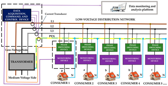
Figure 1. Automatic phase load balancing system architecture for an LV distribution network.

2.2. Mathematical Model of the Proposed PLB Algorithm

Regarding the numerical simulations, to define this algorithm, certain simplifying assumptions were made as follows:

• The line impedances were considered equal and constant along the conductors;
• Consumer loads were regarded as constant at the time of performing the simulation sets;
• Reactive power consumption of loads was not integrated in the model of the proposed PLB algorithm;
• The current flow was considered unidirectional, without the integration of prosumers; the proposed algorithm, in its current form, is designed for passive distribution networks. However, in other related works, bidirectional power flow has been considered and can be found in Ref. [29];
• The algorithm was defined as a topology-independent model.

In the case of solving the problem of phase load unbalance in LV distribution networks of small, medium, or even complex size, rapid convergence, flexibility, and efficiency are the main criteria for obtaining a quality result. The proposed algorithm represents an improved constrained greedy optimization.

A greedy algorithm is a method for solving optimization problems by constructing a solution incrementally, selecting at each step the option that is locally optimal—that is, the choice that provides the maximum immediate gain or the minimum cost. This approach follows the principle of the locally optimal choice. Greedy algorithms do not revise previous decisions and typically produce a single solution that is guaranteed to be locally optimal but not necessarily globally optimal [30,31].

These classic greedy strategies are simple to apply and efficient in many optimization problems. However, for phase load balancing, they may not be sufficiently robust and can lead to local oscillations, where a consumer repeatedly switches between the same two phases without achieving any overall improvement, resulting in local blocking.

On this final consideration, the proposed algorithm introduces the constraint of switching a consumer below an imposed limit. The logic of switching consumers between the three phases considers the effect calculated at each iteration that the movement of a certain consumer produces. At each step, the balancing algorithm chooses the solution that provides the best local result that satisfies the following conditions:

• Compliance with the maximum permissible current limit imposed on the respective conductor;
• The number of times the same consumer is limited to an imposed maximum limit, to avoid local oscillation.

In the algorithm solution model, the stopping criterion is established based on the efficiency of the iterative process (avoiding running the algorithm in situations that bring insignificant improvement). Thus, the stopping criterion is formulated as follows:

3.

Reaching the admissible convergence threshold ($\epsilon$) or performing a predefined maximum number of iterations ($k_{max}$).

2.2.1. Current Unbalance Index ($CUI$)

The standards in force present the evaluation asymmetry factor determined by the negative sequence component. In Romania, regarding the performance standard for the electricity distribution service, it is specified that the negative asymmetry factor should be less than 2%, for 95% of the week, at low and medium voltage.

In the present research, the current asymmetry must be evaluated. Thus, for simplicity and efficiency in calculation, the current unbalance index formula can be used as follows:

$$CUI={\displaystyle \frac{I_{max}-I_{min}}{I_{avg}}},$$

(1)

$$I_{avg}={\displaystyle \frac{I_a+I_b+I_c}{3}},$$

(2)

where $I_a$, $I_b$, $I_c$—the currents of the phases a, b, and c; $I_{max}$—the maximum current among $I_a$, $I_b$, $I_c$; $I_{min}$—the minimum current among $I_a$, $I_b$, $I_c$; $I_{avg}$—the average current.

2.2.2. Defining of Three-Phase Electrical Distribution Network

LV distribution networks are generally configured with three phases and a PEN conductor (Protective Earthed Neutral—which combines protective earth and neutral functions) [32]. For the mathematical model presented in this paper, the conductors are defined as follows: phase a, phase b, phase c, and neutral conductor N. Each single-phase consumer is connected to one of these three phases and requires a certain amount of current, denoted $C_i$, for consumer $i$, at a certain time. Balancing aims to maintain as balanced currents as possible on the three phases, thus reducing excess thermal stress on a particular conductor at a given time and reducing the current on the neutral conductor, implicitly reducing power losses.

2.2.3. Total Current per Phase

Each phase carries a total current equal to the sum of the currents of the consumers connected to that phase. Each consumer has a specified consumption in amperes, and it is associated with a specific phase. Assuming there are n consumers, then the total current on phase j is given by the following equation:

$$I_j={\sum }_{i=1}^n{C}_i·x_{i,j},j\in \left\{a,b,c\right\}.$$

(3)

The binary decision variable is defined as follows:

$$x_{i,j}=\left\{\begin{array}{ll}1,& \mathrm{i}\mathrm{f}\mathrm{t}\mathrm{h}\mathrm{e}\mathrm{c}\mathrm{o}\mathrm{n}\mathrm{s}\mathrm{u}\mathrm{m}\mathrm{e}\mathrm{r}\mathrm{i}\mathrm{i}\mathrm{s}\mathrm{a}\mathrm{s}\mathrm{s}\mathrm{i}\mathrm{g}\mathrm{n}\mathrm{e}\mathrm{d}\mathrm{t}\mathrm{o}\mathrm{p}\mathrm{h}\mathrm{a}\mathrm{s}\mathrm{e}j\\ 0,& \hfill \mathrm{o}\mathrm{t}\mathrm{h}\mathrm{e}\mathrm{r}\mathrm{w}\mathrm{i}\mathrm{s}\mathrm{e}\hfill \end{array}\right.,$$

(4)

where $I_j$—total current on phase j; j $\in \left\{a,b,c\right\}$; $x_{i,j}$—binary decision variable; $I_a$, $I_b$, $I_c$—the currents of the phases a, b, and c; n—the total number of consumers; $C_i$—current consumed by consumer $i$.

As a result, each consumer is connected to exactly one phase. For each phase, it can be written as follows:

$$I_a=\sum _{i=1}^n{C}_i·x_{i,a},$$

(5)

$$I_b=\sum _{i=1}^n{C}_i·x_{i,b},$$

(6)

$$I_c=\sum _{i=1}^n{C}_i·x_{i,c}.$$

(7)

A preliminary and defining step for the proposed algorithm and, in general, for greedy optimization techniques is to identify the maximum current and the minimum current among the three phases of the distribution network:

$$\max \left\{I_a,I_b,I_c\right\},$$

(8)

$$\min \left\{I_a,I_b,I_c\right\}.$$

(9)

The indicator chosen to be minimized at each iteration is the difference between the maximum and minimum currents among the three phases a, phase b, and phase c (current unbalance), respectively, defined as follows:

$${\Delta I}_{max-min}=\underset{j=\left\{a,b,c\right\}}{\max }{I}_j-\underset{j=\left\{a,b,c\right\}}{\min }{I}_j.$$

(10)

2.2.4. Imposed Constraints

In performing PLB in LV distribution networks, it is essential not only to reduce phase current unbalance but also to ensure that the network operates within safe technical limits. Directly moving consumers between phases without considering system constraints may lead to overloaded lines, violation of protection settings, or unstable algorithm behavior. To address these challenges, the proposed approach integrates a set of explicit operational constraints that guide the redistribution process while maintaining system safety. These constraints are represented mathematically in the following form:

• Maximum load limit on phase ($I_j^{max}$).

When redistributing consumers among phases, it is essential to ensure that the maximum allowable current on each phase is not exceeded. By enforcing this constraint, the algorithm guarantees that all consumer reallocations maintain phase currents within the permissible range, ensuring the network operates safely and reliably. Mathematically, this condition is expressed as follows:

$$I_j\le I_j^{max}, j\in \left\{a,b,c\right\},$$

(11)

where $I_j$—total current on phase j; $a,b,c$—distribution network phases.

To ensure electrical safety and compliance during PLB, it is not sufficient to consider only the target phase’s maximum allowable current; each individual consumer reallocation must also be validated against this limit. The condition imposed for a consumer’s switching guarantees that moving the consumer does not cause the phase current to exceed $I_j^{max}$. The condition imposed to validate a consumer’s switching is expressed in the following form:

$$I_j^{(k+1)}{=I}_j^{\left(k\right)}+{C_i}^{i\to {ph}_{min}},$$

(12)

$$I_j^{(k+1)}\le I_j^{max},$$

(13)

where $I_j$–$I_j^{(k+1)}$—current on phase j (iteration $k+1$); $k$—iteration number; ${C_i}^{i\to {ph}_{min}}$—consumption of the consumer that is moved to the minimum load phase; ${ph}_{min}$—minimum load phase; $I_j^{max}$—maximum permissible current limit per phase.

2.

Maximum allowable number of switching operations for each consumer ($S_i^{max}$)

Empirical observations from the simulations revealed that, without limiting the number of reallocations, some consumers could repeatedly switch between phases, causing oscillatory behavior and preventing stable convergence. To mitigate this, a maximum number of switching operations per consumer $S_i^{max}$ was introduced, which, based on the simulation results, empirically eliminated the oscillatory behavior of the objective function and improved the algorithm’s convergence in the simulated cases. This restriction is defined as follows:

$$S_i\le S_i^{max}, \forall i\in \left\{1,\dots n\right\},$$

(14)

where $S_i$—number of switching operations performed on consumer $i$; $S_i^{max}$—maximum allowable number of switching operations for consumer $i$; $n$—total number of consumers.

2.2.5. The Objective Function and Constraints

Therefore, the objective function, representing the difference between the maximum and minimum currents among the three phases, must be minimized at each iteration while respecting the imposed constraints, and is defined as follows:

$$min\left[\underset{jϵ\left\{a,b,c\right\}}{\max }\left(\sum _{i=1}^n{C}_i·x_{i,j}\right)-\underset{jϵ\left\{a,b,c\right\}}{\min }\left(\sum _{i=1}^n{C}_i·x_{i,j}\right)\right],$$

(15)

subject to the constraints defined previously:

$$I_j\le I_j^{max}, j\in \left\{a,b,c\right\},$$

(16)

$$\sum _{i=1}^n{C}_i·x_{i,j}+{C_i}^{i\to {ph}_{min}}\le I_j^{max},$$

(17)

$$S_i\le S_i^{max}, \forall i\in \left\{1,\dots n\right\}.$$

(18)

2.3. Algorithm Implementation

The ICGO algorithm follows a constrained greedy logic. At each iteration, the algorithm evaluates all valid consumer reallocation moves—defined as those that respect defined operational constraints. If a valid move exists, the greedy step will select the move that minimizes current unbalance. The stages of the PLB process are illustrated in the algorithm flowchart in Figure 2, providing an overview of the key steps in the functioning of the proposed ICGO algorithm. Algorithm 1 presents the step-by-step pseudocode of the full decision process.

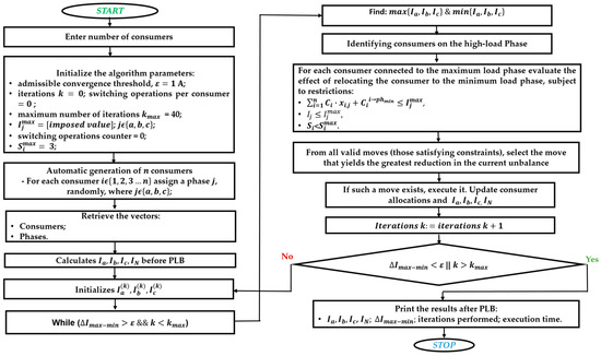
Figure 2. ICGO algorithm—flowchart.

The algorithm procedure consists of the following steps, each explained in detail below as follows:

• Input initialization
  • Enter a valid number of consumers $n$;
  • Set algorithm parameters: maximum number of iterations, maximum allowed switching operations per consumer, convergence threshold $\epsilon$, and maximum load limit on phase $I_j^{max}$.
• Random consumer allocation
  • Consumers are randomly assigned to one of the three phases in the electrical distribution network.
• Initial calculations
  • Calculate the phase currents $I_a$, $I_b$, $I_c$, and the neutral current $I_N$;
  • Initialize iteration counter $k$ = 0 and switching operations counter = 0.
• Main iterative procedure
  • While the stopping criterion is not met
    • Identify the most loaded phase and the least loaded phase;
    • For each consumer connected to the maximum load phase, evaluate the effect of relocating the consumer to the minimum phase load;
    • From all valid moves (those satisfying operational constraints), select the move that yields the greatest reduction in the current unbalance;
    • If such a move exists, execute it, update consumer allocations and phase currents accordingly;
    • Increment the iteration counter $k$ and the switching counter s;
    • Check if the difference between the maximum and minimum currents among the three phases is below the allowable convergence threshold (${\Delta I}_{max-min}\le \epsilon$) or the number of maximum iterations has been reached ($k<k_{max}$); if it is true, consider the balancing terminated. If it is not true, the calculations are resumed.
• Termination
  • Print the results: phase and neutral currents, current unbalance, number of iterations performed, and execution time.

Algorithm 1. ICGO algorithm pseudocode

Input:   n    Number of consumers   ε    Admissible imbalance threshold   $I_j^{max}$   Maximum current allowed on each phase   $k_{max}$   Maximum number of iterations   $S_i^{max}$   Maximum number of allowed switches per consumer

Step 1: Initialization   - $\mathrm{Randomly}\mathrm{assign}\mathrm{consumers}\mathrm{to}\mathrm{one}\mathrm{of}\mathrm{the}\mathrm{three}\mathrm{phases}:\{a,b,c\}$   - $\mathrm{Compute}\mathrm{initial}\mathrm{current}{I}_a$, $I_b$, $I_c$$\mathrm{and}\mathrm{current}\mathrm{unbalance}{\Delta I}_{max-min}$   - $\mathrm{Set}\mathrm{iteration}\mathrm{counter}:k$ ← 0   - $\mathrm{Initialize}\mathrm{switching}\mathrm{counter}\mathrm{for}\mathrm{each}\mathrm{consumer}:S_i$← 0

Step 2: Main Loop   $\mathrm{While}{\Delta I}_{max-min}$$>\mathsf{\epsilon }\mathrm{and}k$$<k_{max}$:     1. Identify       - Phase_max ← Phase with highest current       - Phase_min ← Phase with lowest current     2. For each consumer $i$ assigned to Phase_max:       $\mathrm{If}{S}_i<S_i^{max}$:         - $\mathrm{Simulate}\mathrm{moving}i$ to Phase_min         - Check constraints before calculations:           • $\mathrm{If}\mathrm{new}\mathrm{load}\mathrm{on}\mathrm{Phase}\text{\_}\min \mathrm{after}\mathrm{move}\le I_j^{max}$;           • $\mathrm{And}{S}_i<S_i^{max}$.           Then             - $\mathrm{Compute}\mathrm{new}\mathrm{currents}{I}_a^{\prime }$$,I_b^{\prime }$$,I_c^{\prime }$ after simulated move;             - $\mathrm{Compute}\mathrm{new}\mathrm{current}\mathrm{unbalance}{{\Delta I}_{max-min}}^{\prime }$.     3. If one or more valid moves found       - $\mathrm{Select}\mathrm{the}\mathrm{move}\mathrm{that}\mathrm{minimizes}{{\Delta I}_{max-min}}^{\prime }$       - Perform the selected move:         • Update phase assignments;         • $\mathrm{Update}\mathrm{currents}{I}_a$$,I_b$$,I_c$;         • $\mathrm{Update}{\Delta I}_{max-min}$;         • $\mathrm{Increment}{S}_i$ for the moved consumer.     Else:       - No valid improving move available → Stop     4. Increment iteration counter: $k:=iterationsk+1$.

Step 3: Output   - $\mathrm{Report}:\mathrm{final}\mathrm{phase}\mathrm{currents},\mathrm{final}{\Delta I}_{max-min}$, number of iterations, and switching count.

3. Results and Discussion

In this section, the effectiveness of the proposed ICGO algorithm is analyzed through various sets of numerical simulations for different phase loading scenarios. To appreciate the performance and scalability of the algorithm, three simulation scenarios were developed and simulated in MATLAB R2023b (23.2), with a distinct initial phase current unbalance. The scenarios are the following:

• Scenario A—30 consumers connected to the LV distribution network;
• Scenario B—250 consumers connected to the LV distribution network;
• Scenario C—500 consumers connected to the LV distribution network.

The load balancing results include the following: phase load before and after PLB, current unbalance index before and after PLB, neutral current before and after PLB, the difference between the maximum and minimum current along three phases before and after PLB, algorithm execution time, and number of iterations performed. For detailed evaluation, 20 simulation runs were performed for each scenario. The load balancing results of the first two scenarios will be presented in detail. Also, empirically, for each scenario, the convergence behavior and computational time are evaluated. Finally, the results and conclusions of all the formulated scenarios are comparatively analyzed and presented. For a comprehensive visualization in each iteration of the absolute differences between the maximum and minimum current on the three phases before and after balancing, as well as the corresponding execution times, and number of iterations performed, refer to Appendix A.

Therefore, in this section, the following aspects are reported and discussed:

• Load balancing results for scenario A and scenario B;
  • phase load before and after PLB;
  • current unbalance index before and after PLB;
  • neutral current before and after PLB;
• Empirical evaluation of convergence and time complexity for each scenario;
• Overview of the results: solution quality and algorithm performance.

3.1. Load Balancing Results for Scenario A and Scenario B

3.1.1. Scenario A—30 Consumers Connected to the LV Distribution Network

For this case, 30 consumers with different consumptions were generated, randomly positioned on the three phases. Subsequently, 20 sets of simulations were performed. The results regarding PLB are presented in Table 2, and the data regarding neutral current reduction can be found in Table 3. Also, these results are graphically highlighted in Figure 3 and Figure 4.

Table 2. Numerical simulation results for scenario A—30 consumers.

		Unbalanced Load (A)				Balanced Load (A)
Simulation Run Number	Phase A	Phase B	Phase C	Current Unbalance Index (%)	Phase A	Phase B	Phase C	Current Unbalance Index (%)
1	58.61	58.45	71.9	21.35	62.52	63.2	63.24	1.14
2	58.56	73.51	70.51	22.14	67.23	67.36	67.99	1.13
3	49	64.5	99.41	71.03	71.05	70.83	71.03	0.31
4	80.66	62.6	70.07	25.4	71.05	71.16	71.12	0.15
5	61.9	70.69	43.41	46.5	58.84	58.82	58.34	0.85
6	82.97	56.67	68.63	37.89	69.02	69.03	69.62	0.86
7	82.3	64.5	52.59	44.7	66.54	66.55	66.3	0.38
8	63.84	78.23	72.34	20.13	71.75	71	71.66	1.05
9	67.25	91.41	46.52	65.64	68.49	68.42	68.27	0.32
10	67.25	47.22	96.17	69.72	70.5	69.91	70.23	0.84
11	90.24	71.12	32.07	90.21	64.83	64.57	64.03	1.24
12	39.2	56.46	58.2	37.04	51.41	51.22	51.23	0.37
13	89.27	51.15	36.72	88.99	59.05	58.85	59.24	0.66
14	44.52	82.07	83.1	55.19	69.38	70.24	70.07	1.23
15	41.41	49.29	100.46	92.67	64	63.54	63.62	0.72
16	51.11	62.26	76.91	40.67	63	63.77	63.51	1.21
17	89.83	31.53	73.57	89.72	65.39	64.97	64.57	1.26
18	50.77	81.23	73.47	44.47	68.54	68.96	67.97	1.45
19	79.75	57.98	63.98	32.38	66.95	67.09	67.07	0.21
20	78.75	69.3	57.07	31.71	68.65	68.29	68.18	0.69

Table 3. Neutral current reduction due to phase balancing for scenario A—30 consumers.

Simulation Run Number	Neutral Current Before Balancing (A)	Neutral Current After Balancing (A)	Relative Reduction in Neutral Current (%)
1	13.37	0.7	94.76
2	13.7	0.7	94.89
3	44.72	0.21	99.53
4	15.72	0.1	99.36
5	24.12	0.49	97.97
6	22.81	0.61	97.33
7	25.9	0.25	99.03
8	12.53	0.71	94.33
9	38.91	0.19	99.51
10	42.62	0.51	98.8
11	51.35	0.71	98.62
12	18.19	0.19	98.96
13	47.03	0.34	99.28
14	38.08	0.79	97.93
15	55.53	0.43	99.23
16	22.41	0.68	96.97
17	52.11	0.71	98.64
18	27.42	0.86	96.86
19	19.64	0.13	99.34
20	18.83	0.43	97.72

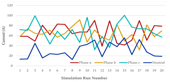
Figure 3. Phase currents and neutral current before PLB—scenario A (30 consumers).

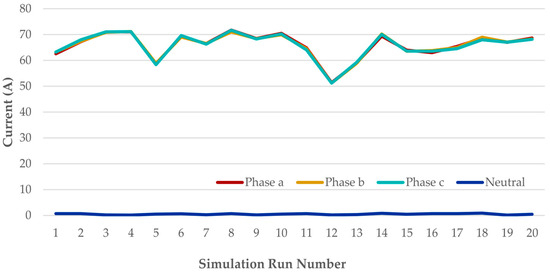
Figure 4. Phase currents and neutral current after PLB—scenario A (30 consumers).

As can be seen in Table 2 and Table 3 and Figure 3, the set of simulations performed presents various degrees of asymmetry and, implicitly, a distinct neutral current as shown below.

• Simulation number 11—a degree of current unbalance index of 90.21% and a neutral current of 51.35 A;
• Simulation number 13—a degree of current unbalance index of 88.99% and a neutral current of 47.03 A;
• Simulation number 17—a degree of current unbalance index of 89.72% and a neutral current of 52.11 A;
• Simulation number 15 presents the highest current unbalance index of 92.67%, and the neutral current of 55.53 A exceeds the values of the currents on phase a and phase b, respectively.

Significant degrees of asymmetry of the currents and neutral current values exceed the current value on phase c can be noted.

After PLB, Figure 4 presents a favorable situation, where the currents are approximately equal per phase, and the current on the neutral approaches zero, below 1 A. Thus, for simulation number 15 (the strongest asymmetry), a reduction in the current unbalance index from 92.67% to 0.72% is observed, and a decrease in the neutral current from 55.53 A to 0.43 A.

3.1.2. Scenario B—250 Consumers Connected to the LV Distribution Network

For this scenario, the number of consumers was increased from 30 to 250 consumers. The evolution of the phase and neutral currents throughout the simulations is highlighted numerically in Table 4 and Table 5, and graphically in Figure 5 and Figure 6.

Table 4. Numerical simulation results for scenario B—250 consumers.

		Unbalanced Load (A)				Balanced Load (A)
Simulation Run Number	Phase A	Phase B	Phase C	Current Unbalance Index (%)	Phase A	Phase B	Phase C	Current Unbalance Index (%)
1	609.75	593.15	534.06	13.07	579.13	579.26	578.57	0.12
2	597.22	611.91	535.05	13.22	581.49	581.48	581.21	0.05
3	625.17	504.1	596.5	21.05	574.63	575.55	575.59	0.17
4	582.71	490.04	581.19	16.81	550.9	551.53	551.51	0.11
5	566.4	540.31	608.85	11.99	571.52	571.55	572.49	0.17
6	514.98	629.4	621.93	19.43	588.7	589.02	588.59	0.07
7	584.98	588.62	491.07	17.58	555.09	554.49	555.09	0.11
8	536.14	532.16	522.09	2.65	530.48	530.03	529.88	0.11
9	572.93	514.61	632.58	20.57	572.93	573.55	573.64	0.12
10	572.93	573.55	573.64	0.12	555.14	555.78	554.9	0.15
11	599.88	539.79	597.85	10.38	578.72	579.38	579.42	0.12
12	614.11	507.88	571.34	18.82	564.2	564.56	564.57	0.07
14	635.79	548.44	509.83	22.31	564.56	564.98	564.52	0.08
14	551.56	557.1	501.76	10.31	537.08	536.68	536.66	0.08
15	561.21	509.89	550.26	9.5	540.77	539.88	540.71	0.16
16	520.11	654.04	571.47	23.02	581.47	581.83	582.32	0.15
17	562.59	609.61	476.33	24.25	549.9	549.3	549.33	0.11
18	624.57	558.31	527.45	17.04	570.5	570.19	569.64	0.15
19	485.94	618.3	501.13	24.73	535.66	534.89	534.82	0.16
20	506.95	618.53	604.69	19.35	576.43	576.51	577.23	0.14

Table 5. Neutral current reduction due to phase balancing for scenario B—250 consumers.

Simulation Run Number	Neutral Current before Balancing (A)	Neutral Current after Balancing (A)	Relative Reduction in Neutral Current (%)
1	68.91	0.64	99.07
2	70.67	0.28	99.6
3	109.58	0.94	99.14
4	91.92	0.62	99.33
5	59.92	0.96	98.4
6	110.87	0.39	99.65
7	95.78	0.6	99.37
8	12.54	0.54	95.69
9	102.17	0.67	99.34
10	68.46	0.79	98.85
11	59.1	0.68	98.85
12	92.58	0.37	99.6
13	111.77	0.44	99.61
14	52.79	0.41	99.22
15	46.82	0.86	98.16
16	117.03	0.74	99.37
17	117.08	0.59	99.5
18	85.95	0.75	99.13
19	125.46	0.81	99.35
20	105.34	0.76	99.28

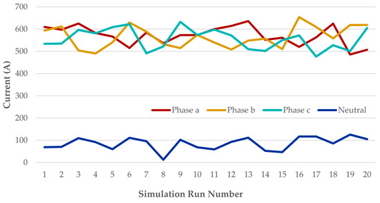
Figure 5. Phase currents and neutral current before PLB—scenario B (250 consumers).

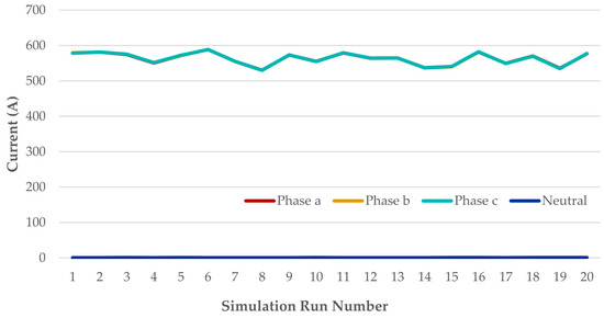
Figure 6. Phase currents and neutral current after PLB—scenario B (250 consumers).

Based on the simulations performed, the initial current unbalance index presents high values for the following: simulation number 14 (22.31%), simulation number 16 (23.02%), simulation number 17 (24.25%), and simulation number 19 (24.73%). Obviously, the neutral current registers the highest absolute value in simulation number 19 (125.46 A), as shown in Table 5. Also, the relative reduction in the neutral current is in percentage values between 98.16% and 99.65%, except for simulation number 8, where the reduction in the neutral current is 95.69%, but the initial current unbalance index in that simulation has a reduced value (2.65%), as shown in Table 4. It can be concluded that the effectiveness of the algorithm remains high despite the fact that the number of consumers was increased from 30 to 250.

3.2. ICGO Algorithm: Empirical Analysis of the Convergence and Time Complexity

The analysis of the obtained results included the following efficiency parameters: the difference between the maximum and minimum currents among the three phases before and after PLB, current unbalance index, neutral current reduction, execution time, and the number of switching operations performed for PLB.

In this stage, the empirically derived convergence model obtained after running the proposed algorithm is presented, as well as the estimation complexity of the execution time.

3.2.1. ICGO Algorithm: Empirically Derived Convergence Model and Computational Framework

The following subsection presents an empirical formulation of the convergence and computational behavior of the proposed ICGO algorithm. This model was derived from an empirical analysis, based on the observed behavior of the algorithm on various datasets. This formulation does not represent formal mathematical proof of convergence.

Furthermore, the proposed algorithm employs a greedy strategy, selecting at each iteration the locally optimal consumer move that minimizes current unbalance at iteration k (for simplicity, the difference between the maximum current and the minimum current at iteration $k$ is hereafter denoted by ${\Delta }_k$); thus

$${\Delta }_k=\underset{j=\left\{a,b,c\right\}}{\max }{I_j}^{\left(k\right)}-\underset{j=\left\{a,b,c\right\}}{\min }{I_j}^{\left(k\right)},$$

(19)

where ${I_j}^{\left(k\right)}$—the current on phase $j$ at iteration $k$.

At each iteration, the algorithm evaluates all valid consumer reallocation moves—defined as those that respect operational constraints. If valid moves exist, the greedy step will select the one that minimizes ${\Delta }_{k+1}$.

In particular, numerical simulations revealed a specific edge case in which the algorithm exhibited oscillatory behavior, caused by a consumer being repeatedly reallocated between two phases. In such scenarios, the sequence ${\Delta }_k$ failed to progress, instead alternating between two constant values, where $k_0\in \mathbb{N}$ is the first iteration at which the oscillatory behavior begins to repeat periodically:

$${\Delta }_{k+2}={\Delta }_{k,}\forall k\ge k_0.$$

(20)

This periodic behavior breaks the required monotonic decrease in ${\Delta }_k$, preventing numerical convergence to a unique limit.

To mitigate such behavior, an empirical stabilization constraint was introduced, limiting each consumer $i$ to a maximum number of reallocations $S_i\le S_i^{max}=3$ during the entire balancing process. The maximum of three reallocations per consumer was chosen based on observations from tests conducted on various datasets. This restriction proved sufficient to eliminate cycles and ensure algorithm stabilization without adversely affecting the solution quality. After introducing this constraint, the empirical results indicate that the sequence ${\Delta }_k$ exhibited a non-increasing and non-oscillatory behavior, the monotonic decrease in ${\Delta }_k$ in all datasets performed as follows:

$${\Delta }_{k+1}\le {\Delta }_k,$$

(21)

so that the sequence ${\left({\Delta }_k\right)}_{kϵ\mathbb{N}}$ appears as a monotonically non-increasing sequence to a fixed point ${\Delta }^{*}$ bounded below by zero:

$${\Delta }_k\to {\Delta }^{*}\ge 0.$$

(22)

While this constraint effectively suppressed oscillations in all tested scenarios, it does not constitute a formal guarantee that cycles cannot occur in other configurations. In practical terms, the stopping condition for the proposed PLB model is as follows:

$${\Delta }_k\le \epsilon , \epsilon \le 1 \mathrm{A},$$

(23)

where $\epsilon$ is the admissible convergence threshold.

However, a rigorous theoretical guarantee is that ${\Delta }^{*}\le \epsilon$ cannot be established in the general case. This limitation arises because, in certain system configurations, no further valid moves exist, or the maximum number of iterations has been reached. In such cases, the algorithm may stop to a fixed point ${\Delta }^{*}$ as follows:

$${\Delta }_k\to {\Delta }^{*}>\epsilon .$$

(24)

Nevertheless, empirical experiments consistently showed that the iterative process stabilizes after a finite number of iterations and that ${\Delta }_k$ reaches a steady value ${\Delta }^{*},$ satisfying ${\Delta }_k\le \epsilon$, for all tested scenarios.

Despite the absence of formal proof guaranteeing convergence to $\Delta \le \epsilon$, all conducted numerical simulations showed that the algorithm reliably achieved convergence within the admissible threshold. These results are provided in the results section.

The threshold $\epsilon$ was empirically chosen to balance the computational cost and solution quality. Lowering $\epsilon$ increases the number of iterations significantly, often with diminishing returns in performance, especially across diverse datasets. By decreasing the admissible convergence threshold, the computational cost will increase (on different datasets, mainly the number of iterations has increased).

3.2.2. Empirical Estimation of Time Complexity

The mathematical notation $O\left(n\right)$ describes the algorithmic complexity. More precisely, it evaluates the increase in the execution time of an algorithm as the size of the input data increases. Applying the following model to the observed execution times for different input sizes (e.g., 30 to 250 consumers), an empirical complexity order $k$ was obtained.

The empirical time complexity of the proposed algorithm was estimated assuming the execution time follows the form:

$$T\left(n\right)=a·n^k,$$

(25)

where $n$ is the input size, $a$ is a constant, and $k$ is the complexity order to be determined. Given two measurements of execution times $T_1$ and $T_2$ corresponding to input sizes $n_1$ and $n_2$, respectively, the relationship can be expressed as follows:

$${\displaystyle \frac{T_2}{T_1}}={\left({\displaystyle \frac{n_2}{n_1}}\right)}^k.$$

(26)

Taking the logarithm of both sides leads to the following:

$$k={\displaystyle \frac{\log \left(T_2/T_1\right)}{\log \left(n_2/n_1\right)}}.$$

(27)

The empirical convergence model presented in this section was derived from the observed behavior of the algorithm under various operating conditions presented in the previous subsection.

The following subsection provides the detailed numerical results that served as the empirical basis for this formulation.

3.3. ICGO Algorithm: Numerical Results of the Algorithm’s Convergence, Execution Time Estimation, and Sensitivity of Convergence Threshold

This subsection presents the numerical results of the algorithm’s convergence, execution time estimation, and sensitivity analysis of convergence threshold $\epsilon$ across all simulated scenarios: 30 consumers (scenario A), 250 consumers (scenario B), and 500 consumers (scenario C) connected to the LV distribution network. In Table 6, the parameters defined and used in the ICGO algorithm are presented, as well as the numerical values chosen for each of them.

Table 6. Defined parameters used in the proposed ICGO algorithm.

Parameter	Symbol	Value
Admissible convergence threshold	$\epsilon$	1 A 1
Maximum allowable number of switching operations for consumer i	$S_i^{max}$	3
Maximum number of iterations	$k_{max}$	40

¹ A—ampere.

3.3.1. Empirical Evaluation of Convergence—Scenario A (30 Consumers)

In this case, rapid convergence is observed, with rapid acceleration as the values decrease, as shown in Table 7 and Figure 7. A decrease in value ${\Delta I}_{max-min}$ of approximately 41% can be observed in the second iteration, followed by a decrease of approximately 70%, to finally obtain a value very close to the horizontal asymptote (zero value), hence a decrease of 99%.

Table 7. The evolution of the objective function over the iterations—30 consumers.

Number of Iteration	The Number of Consumers Switched	${\Delta \mathit{I}}_{\mathit{m}\mathit{a}\mathit{x}-\mathit{m}\mathit{i}\mathit{n}}$ 1 (A)	Decrease from the Previous Iteration (%)	Observations
1	17	35.63	-	Initial value
2	30	20.95	41.2%	Strong decrease
3	26	6.36	69.7%	High-rate decrease
4	19	0.05	99.2%	Convergence

¹ ${\Delta I}_{max-min}$—the difference between the maximum and minimum currents among the three phases (current unbalance).

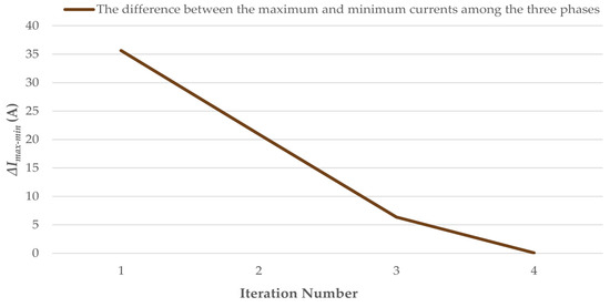
Figure 7. Convergence of the numerical solution in time—scenario A (30 consumers).

The data indicate a high efficiency of the proposed algorithm, the final difference between the maximum and minimum currents among the three phases’ value being 0.05 A.

Also, the values of the phase currents before and after PLB are presented in Table 8. After PLB, a favorable situation can be seen—approximately equal loads on the three phases as follows: phase a (61.46 A), phase b (61.41 A), and phase c (61.45 A).

Table 8. Phase loads before and after PLB—scenario 30 consumers.

Phase	Initial Phase Load (A)	Final Phase Load (A)
a	24.43	61.46
b	70.33	61.41
c	87.56	61.45

3.3.2. Empirical Evaluation of Convergence—Scenario B (250 Consumers)

This case presents a decrease in the ${\Delta I}_{max-min}$ value that is more uniform, and the convergence is more gradual than in the previous case, as can be seen in the first five iterations according to Table 9 and Figure 8. Starting with iteration number 6, a significant decrease in the value can be observed, by 79.19%, an acceleration of convergence and, therefore, culminating in its achievement in iteration 9.

Table 9. The evolution of the objective function over the iterations—scenario B (250 consumers).

Number of Iteration	The Number of Consumers Switched	${\mathit{\Delta }\mathit{I}}_{\mathit{m}\mathit{a}\mathit{x}-\mathit{m}\mathit{i}\mathit{n}}$ 1 (A)	Decrease from the Previous Iteration (%)	Observations
1	250	110.31	-	Initial value
2	220	85.19	22.77	Initial decrease
3	211	60.43	29.10	Increased decrease
4	120	35.85	40.68	Significant decrease
5	125	16.29	54.54	High-rated decrease
6	26	3.39	79.19	Strong decrease
7	219	1.77	47.78	Moderate decrease
8	5	1.01	42.94	Moderate decrease
9	20	0.12	88.12	Convergence

¹ ${\Delta I}_{max-min}$—the difference between the maximum and minimum currents among the three phases (current unbalance).

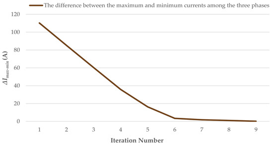
Figure 8. Convergence of the numerical solution in time—scenario B (250 consumers).

The quality of the solution obtained after PLB is also high. The phase currents are very close, as shown in Table 10, with a final difference between the maximum and minimum currents among the three phases resulting in an absolute value of 0.12 A.

Table 10. Phase loads before and after PLB—scenario 250 consumers.

Phase	Initial Phase Load (A)	Final Phase Load (A)
a	617.23	545.99
b	481.78	546.06
c	538.98	545.94

3.3.3. Empirical Evaluation of Convergence—Scenario C (500 Consumers)

In this last simulated scenario, a total convergence, not semi-optimal, can be noted in Table 11 and Figure 9. Compared to the previous cases, the convergence process is gradual, approaching a linear shape, but it keeps its speed. The first 4–5 iterations show a moderate but progressive decrease, following a more accelerated decreasing rhythm from iteration 7 to iteration 10 (in iteration 9, percentage value exceeding 20%). The last three iterations show a significant and defining decrease for reaching convergence. Qualitatively, the final value of ${\Delta I}_{max-min}$, noted as 0.04 A, approaches the horizontal asymptote, which indicates the performance of the ICGO even on a large number of consumers.

Table 11. The evolution of the objective function over the iterations—scenario C (500 consumers).

Number of Iteration	The Number of Consumers Switched	${\Delta \mathit{I}}_{\mathit{m}\mathit{a}\mathit{x}-\mathit{m}\mathit{i}\mathit{n}}$ 1 (A)	Decrease from the Previous Iteration (%)	Observations
1	254	227.46	-	Initial value
2	453	214.09	5.87	Slow decrease
3	306	189.02	11.73	Increased decrease
4	103	175.59	7.11	Moderate decrease
5	197	150.78	14.13	Significant decrease
6	359	137.54	8.77	Moderate decrease
7	67	112.76	18.01	High-rate decrease
8	153	99.65	11.65	Stable decrease
9	491	74.98	24.74	Significant decrease
10	495	61.95	17.38	Stable decrease
11	138	37.33	39.75	Strong decrease
12	477	24.43	34.55	Strong decrease
13	469	0.04	99.84	Total convergence

¹ ${\Delta I}_{max-min}$—the difference between the maximum and minimum currents among the three phases (current unbalance).

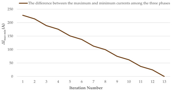
Figure 9. Convergence of the numerical solution in time—scenario C (500 consumers).

As can be seen in Table 12, an optimal balance was obtained in this case, the values of the phase currents being equal after PLB.

Table 12. Phase loads before and after PLB—scenario 500 consumers.

Phase	Initial Phase Load (A)	Final Phase Load (A)
a	1205.2	1129.7
b	1218.6	1129.7
c	965.37	1129.7

3.3.4. Empirical Determination of Time Complexity

Applying (25)–(27) to the observed execution times for different input sizes (30 to 250 consumers), an empirical complexity order of approximately $k=0.76$ was obtained, indicating sub-linear time complexity in this range. For larger input sizes (250 to 500 consumers), a similar calculation yielded $k=2.16$, consistent with quadratic complexity. Based on the observed runtime over various input sizes, the empirical time complexity appears to lie between sub-linear and quadratic on simulated cases. This estimation is empirical and does not constitute a formal theoretical analysis.

Thus, it can be seen in Table 13 and Figure 10 that when the network size increases by about 8.33 times (from 30 to 250 consumers), the execution time increases by about 5 times. In linear terms, it should have increased by 8.33 times. The roughly 5-fold increase remains asymptotically better than the linear time. Thus, in this case, the empirical time complexity algorithm follows approximately a sub-linear polynomial trend, calculated as $O\left(n^{0.76}\right).$ From 250 to 500 consumers, the increase is twofold, but the execution time increased by about 4.5 times, which indicates an approximately quadratic increase, $O\left(n^{2.16}\right)$.

Table 13. Evolution of the algorithm execution time with the increase in the number of consumers.

Increasing the Number of Consumers	Execution Time (s)	The Network Size Increasing $(\times \mathbf{T}\mathbf{i}\mathbf{m}\mathbf{e}\mathbf{s}$)	Execution Time Increasing	$\mathit{k}$ 1	Time Complexity	Observations— Time Complexity
30–250	0.00051–0.00257	~8.33×	5.04×	≈0.76	$O(n^{0.76}$)	sub-linear 2
250–500	0.00257–0.01149	2×	4.47×	≈2.16	$O\left(n^{2.16}\right)$	~quadratic 3

¹ k—complexity order, $O(n^k$). ² sub-linear: $O(n^k$), $0<k<1$. ³ quadratic: $O(n^k$), $k=2$.

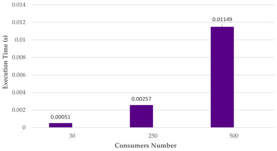
Figure 10. Execution time of the proposed PLB algorithm for all simulated scenarios.

Theoretical time complexities for certain standard algorithms are available in the specialized literature. While these values are generally applicable, they may vary from slight to significant differences depending on the specific implementation, parameter settings, and adaptations introduced. In Table 14 the approximate time complexity of various algorithms is presented compared to the empirical execution time of the proposed algorithm [33,34,35,36,37,38,39,40].

Table 14. Approximate time complexity of various algorithms—comparison.

Algorithm	Time Complexity	Execution Time (Reference)
ICGO (proposed)	$O\left(n^{0.76}\right)$$,O\left(n^{2.16}\right)$ 1	1× (reference)
Classic Greedy	$O\left(n\right)$	~10× faster
GA	$O(G\times P\times n)$ 2	~3–5× slower
PSO	$O(M\times I\times n)$ 3	~2–4× slower
Brute Force	$O\left(3^n\right)$	~<1000× slower (impractical)

¹ $n$—input data (number of consumers); $O\left(n^{0.76}\right)$, for 30–250 consumers range (empirically); $O\left(n^{2.16}\right)$, for 250–500 consumers range (empirically). ² $G$—the number of generations; $P$—population size. ³ $M$—the number of particles; $I$—the number of iterations.

3.3.5. Sensitivity Analysis of Convergence Threshold $\epsilon$

A sensitivity analysis of the parameter $\epsilon$ on the number of iterations was performed. Table 15 summarizes the average performance of the algorithm over 20 numerical simulations for each convergence threshold (ε = 0.5 A, 1 A, and 2 A) under all defined scenarios (A, B, C). It can be observed that $\epsilon =1$ A provides a compromise between convergence speed and numerical stability.

Table 15. Algorithm convergence and computational performance for different admissible threshold (ε) values.

Scenario	$\mathit{\epsilon }$ 2 (A)	Number of Iterations	Execution Time (s)	${\Delta \mathit{I}}_{{\mathit{m}\mathit{a}\mathit{x}-\mathit{m}\mathit{i}\mathit{n}}_1}$ 1 (A)	Observations— Objective Function
A	0.5	21	0.00268	2.46	No convergence
	1	4	0.00051	0.52	Convergence achieved
	2	6	0.00101	1.38	Convergence achieved
B	0.5	18	0.02958	0.49	Oscillatory behavior
	1	6	0.00257	0.67	Convergence achieved
	2	9	0.0074	1.34	Convergence achieved
C	0.5	17.05	0.039855	0.40	Convergence achieved
	1	11	0.01149	0.68	Convergence achieved
	2	13	0.066165	1.10	Convergence achieved

¹ ${\Delta I}_{{max-min}_1}$—final difference between the maximum and minimum currents among the three phases (final current unbalance). ² $\epsilon$—admissible convergence threshold.

When a small value ($\epsilon$ $=$0.5 A) was used, the algorithm exhibited an excessive number of iterations (17–21) and an increase in the execution time. Moreover, the oscillatory behavior of the objective function ${\Delta I}_{max-min}$ was observed in scenarios A and B, where the unbalance alternated between two close values. This indicates that the algorithm continued to reassign individual consumers between phases without achieving a meaningful improvement in the objective value. Hence, a too restrictive convergence threshold made the process overly sensitive to small local variations, resulting in oscillatory behavior or slow convergence.

At the opposite extreme, for $\epsilon$ $=$ 2 A, the algorithm converged rapidly and stably in all cases but produced noticeably higher residual unbalances (${\Delta I}_{max-min}=$ 1.1–1.38 A). Although computational times remained low, the larger threshold allowed the algorithm to terminate prematurely, before reaching a sufficiently balanced phase configuration. Thus, the solution quality degraded despite apparent convergence.

In contrast, setting $\epsilon$ $=$ 1 A provided consistent and reliable performance across all tested scenarios. The algorithm converged within 4–11 iterations, with minimal execution times (0.0005–0.011 s) and achieved a final current unbalance below 0.69 A. No oscillations were observed, and the decrease in the objective function was monotonic in every case. These results indicate that the 1 A threshold effectively filters out insignificant fluctuations while preserving enough sensitivity to further improve the PLB when real improvements are possible.

Therefore, the empirical evidence supports ε = 1 A as the suitable convergence threshold, since it achieves the best trade-off between stability, accuracy, and computational efficiency. It ensures convergence in all tested scenarios while maintaining a sufficiently low final current unbalance without unnecessary iterations. These trends and observations are further illustrated in Figure 11, Figure 12 and Figure 13, which graphically depict the final current unbalance, number of iterations, and execution time for each scenario and convergence threshold.

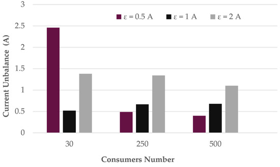
Figure 11. Current unbalance across scenarios for different convergence thresholds.

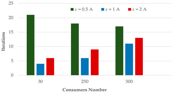
Figure 12. Number of iterations across scenarios for different convergence thresholds.

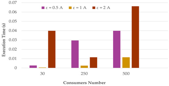
Figure 13. Execution time across scenarios for different convergence thresholds.

3.4. Overview of the Results: Solution Quality and Algorithm Performance

The overall results of the numerical simulations for all scenarios defined after the PLB process are found in Table 16. The table presents the average value of all 20 datasets corresponding to each simulated scenario. In Figure 14, it can be seen that, relatively, the algorithm is more efficient as the number of consumers increases. The current unbalance index approaches zero for the scenarios with 250 ($CUI=0.12\%$) and 500 consumers ($CUI$ = $0.0605\%$). The data are reported to the average current in each case.

Table 16. Summary table regarding the average values of the proposed algorithm performance results for each scenario.

Scenario	Number of Consumers	${\mathit{C}\mathit{U}\mathit{I}}_{0,\mathit{m}\mathit{e}\mathit{d}}$ 1	${\mathit{C}\mathit{U}\mathit{I}}_{1,\mathit{m}\mathit{e}\mathit{d}}$ 2	${\mathit{R}\mathit{I}}_{\mathit{m}\mathit{e}\mathit{d}}$ 3	${\Delta \mathit{I}}_{{\mathit{m}\mathit{a}\mathit{x}-\mathit{m}\mathit{i}\mathit{n}}_{0,\mathit{m}\mathit{e}\mathit{d}}}$ 4	${\Delta \mathit{I}}_{{\mathit{m}\mathit{a}\mathit{x}-\mathit{m}\mathit{i}\mathit{n}}_{1,\mathit{m}\mathit{e}\mathit{d}}}$ 5	$\mathit{T}$ 6	Iterations
A	30	51.3775	0.8035	97.953	33.6875	0.521052632	0.00051	4
B	250	15.81	0.12	99.0255	93.233	0.677	0.00257	6
C	500	16.091	0.0605	99.5335	182.405	0.6865	0.01149	11

¹ ${CUI}_{0,med}$—initial average current unbalance for all datasets. ² ${CUI}_{1,med}$—final average current unbalance for all datasets. ³ ${RI}_{med}$—neutral current reduction (average value of datasets). ⁴ ${\Delta I}_{{max-min}_{0,med}}$—the initial average value of difference between the maximum and minimum currents among the three phases for all datasets. ⁵ ${\Delta I}_{{max-min}_{1,med}}$—the final average value of difference between the maximum and minimum currents among the three phases for all datasets. ⁶ $T$—the average value of execution time.

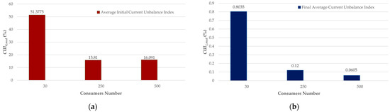
Figure 14. (a) Average initial current unbalance index for all scenarios; (b) final average current unbalance index for all scenarios.

Also, the relative reduction in the neutral current is close to the optimal solution, as shown in Figure 15, and the values can be noted in Table 16 as follows: for the scenario with 30 consumers (97.953%,), for the scenario with 250 consumers (99.0255%,), and for the scenario with 500 consumers (99.5335%.) These results highlight the efficiency and accuracy of the ICGO proposed.

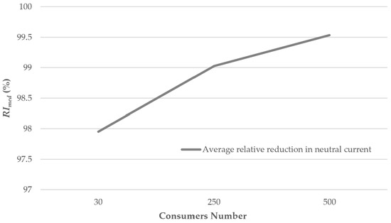
Figure 15. Average relative reduction in neutral current for all scenarios simulated.

It can be concluded that the algorithm converges to the solution and, implicitly, obtains results near to a perfect balance for all defined and simulated scenarios, but with higher computational costs as the number of consumers increases, as can be seen in Figure 16. However, overall, the number of iterations performed is extremely low compared to the other algorithms proposed in the specialized literature presented at the beginning of the paper.

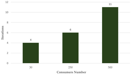
Figure 16. The average number of iterations performed in the simulation sets of each scenario.

4. Conclusions and Future Work

In the context of the modernization of electrical distribution networks, it can be concluded that APLB systems are a necessity, but undoubtedly a complex objective. This paper aims to present an improved constrained greedy algorithm—practical, efficient, and with a reduced computational cost. This proposed PLB algorithm has the following advantages: can be easily applied in an electrical distribution network; is more efficient in terms of computing resources, processing time, and, for practical situations, offers a satisfactory solution, in a relatively short time with a reduced number of iterations; convergence is ensured in all operating scenarios simulated; the proposed algorithm strikes a balance between solution performance and computational cost; the algorithm exhibits scalability, as evidenced by various numerical simulations with different numbers of consumers; and flexibility in implementation allows improving the algorithm through various hybrid approaches.

The results obtained highlight the quality of the solution, but also the computational performance of the proposed PLB algorithm: Neutral current after PLB below 0.63 A in all simulations, reduced number of iterations (4 iterations in the operating scenario with 30 consumers and 11 iterations in the operating scenario with 500 consumers), and increased convergence speed (0.00051 s—execution time for 30 consumers scenario; 0.01149 s—execution time for 500 consumers scenario).

From the point of view of practical implications, the proposed model is simple to implement and flexible, which allows its further improvement in terms of robustness, convergence, and scalability. Despite these findings, this paper makes a significant contribution to the research on the non-symmetric regime of operation of the electrical distribution network and proposes an efficient alternative for its solution.

Regarding future work, the proposed goal is to improve the present algorithm and test it on a developed physical PLB model. While the algorithm exhibits strong empirical convergence, establishing formal theoretical guarantees remains a priority for future research. Despite some current aspects such as empirically estimated time complexity, empirical evaluation of convergence, simplified simulation scenarios, static load assumptions, and the lack of identical or sufficiently similar datasets for direct comparison with other algorithms, the proposed ICGO demonstrates significant and promising performance, efficiently reducing current unbalance while maintaining computational performance.

Future work will focus on addressing certain aspects as follows: testing the algorithm on the experimental setup to evaluate hardware-related effects, extending simulations to dynamic loads and more complex network topologies, and optimizing the sampling interval adaptively according to real consumption patterns. Additionally, further algorithmic refinements will enhance performance while preserving stability. Overall, these directions ensure that the ICGO can evolve into a robust and practically applicable solution for real-world LV distribution networks.

References

- Al-Jaafreh, M.A.A.; Mokryani, G. Planning and operation of LV distribution networks: A comprehensive review. IET Energy Syst. Integr. 2019, 1, 133–146. [Google Scholar] [CrossRef]
- Ochoa, L.F.; Ciric, R.M.; Padilha-Feltrin, A.; Harrison, G.P. Evaluation of distribution system losses due to load unbalance. In Proceedings of the 15th Power Systems Computation Conference (PSCC 2005), Liège, Belgium, 14–18 August 2005; pp. 1–4. [Google Scholar]
- Gheorghe, S.; Postolache, P.; Ene, S.; Ivan, M.; Brănescu, V.; Mihăescu, M. Monitoring of Electric Power Quality, 2nd ed.; Macarie Publishing House: Târgoviște, Romania, 2001; pp. 138–141. [Google Scholar]
- Tavakoli Bina, M.; Kashefi, A. Three-phase unbalance of distribution systems: Complementary analysis and experimental case study. Int. J. Electr. Power Energy Syst. 2011, 33, 817–826. [Google Scholar] [CrossRef]
- Ma, K.; Fang, L.; Kong, W. Review of Distribution Network Phase Unbalance: Scale, Causes, Consequences, Solutions, and Future Research Direction. CSEE J. Power Energy Syst. 2020, 6, 479–488. [Google Scholar] [CrossRef]
- Toader, C.; Porumb, R.; Bulac, C.; Tristiu, I. A Perspective on Current Unbalance in Low Voltage Distribution Networks. In Proceedings of the 2015 9th International Symposium on Advanced Topics in Electrical Engineering (ATEE), Bucharest, Romania, 7–9 May 2015; pp. 741–746. [Google Scholar] [CrossRef]
- Antić, T.; Capuder, T.; Bolfek, M. A Comprehensive Analysis of the Voltage Unbalance Factor in PV and EV Rich Non-Synthetic Low Voltage Distribution Networks. Energies 2021, 14, 117. [Google Scholar] [CrossRef]
- Najafi Zanjani, P.; Javadi, S.; Hosseini Aliabadi, M.; Gharehpetian, G.B. A Novel Approach for Mitigating Electrical Losses and Current Unbalance in Low Voltage Distribution Networks. IET Gener. Transm. Distrib. 2025, 19, e70072. [Google Scholar] [CrossRef]
- Matanov, N.; Angelov, I.; Stoev, P. A Study of Load Unbalance on Low Voltage Grid. In Proceedings of the 2024 16th Electrical Engineering Faculty Conference (BulEF), Varna, Bulgaria, 19–22 September 2024; pp. 1–5. [Google Scholar] [CrossRef]
- El-Hawary, M.E.; Marei, M.I.; Mohamed, A.A.S. Techniques for Compensation of Unbalanced Conditions in LV Distribution Networks with Integrated Renewable Generation: An Overview. Electr. Power Syst. Res. 2023, 214, 108932. [Google Scholar] [CrossRef]
- Hao, H.; Xu, C.; Zhang, W.; Chen, X.; Yang, S.; Muntean, G.-M. Reliability-aware Optimization of Task Offloading for UAV-assisted Edge Computing. IEEE Trans. Comput. 2025, 74, 3832–3844. [Google Scholar] [CrossRef]
- Khan, A.; Ali, M. Three-Phase Load Balancing in Distribution Systems Using Load Sharing Technique. Eng. Proc. 2023, 46, 18. [Google Scholar] [CrossRef]
- Bao, G.; Ke, S. Load Transfer Device for Solving a Three-Phase Unbalance Problem Under a Low-Voltage Distribution Network. Energies 2019, 12, 2842. [Google Scholar] [CrossRef]
- Ivanov, O.; Neagu, B.-C.; Gavrilas, M.; Grigoras, G.; Sfintes, C.-V. Phase Load Balancing in Low Voltage Distribution Networks Using Metaheuristic Algorithms. In Proceedings of the 2019 International Conference on Electromechanical and Energy Systems (SIELMEN), Craiova, Romania, 9–11 October 2019; pp. 1–6. [Google Scholar] [CrossRef]
- El Hassan, M.; Najjar, M.; Tohme, R.; Daba, J.; Ayoubi, R. Implementation and Testing of a Practical Product to Balance Single-Phase Loads in a Three-Phase System at the Distribution and Unit Levels. Renew. Energy Power Qual. J. 2023, 21, 323. [Google Scholar] [CrossRef]
- Zhang, C.; Nie, P.; Zhang, H.; Ji, K. Research on Three-Phase Imbalance Control Strategy of Low-Voltage Distribution Station Area. In Proceedings of the 2022 China International Conference on Electricity Distribution (CICED), Changsha, China, 7–8 September 2022; pp. 941–946. [Google Scholar] [CrossRef]
- Grigoraș, G.; Neagu, B.-C.; Gavrilaș, M.; Triștiu, I.; Bulac, C. Optimal Phase Load Balancing in Low Voltage Distribution Networks Using a Smart Meter Data-Based Algorithm. Mathematics 2020, 8, 549. [Google Scholar] [CrossRef]
- Toma, N.; Ivanov, O.; Neagu, B.; Gavrila, M. A PSO Algorithm for Phase Load Balancing in Low Voltage Distribution Networks. In Proceedings of the 2018 International Conference and Exposition on Electrical and Power Engineering (EPE), Iasi, Romania, 18–19 October 2018; IEEE: Iasi, Romania, 2018; pp. 857–862. [Google Scholar]
- Zhao, J.; Wang, C.; Zhao, B.; Lin, F.; Zhou, Q.; Wang, Y. A review of active management for distribution networks: Current status and future development trends. Electr. Power Compon. Syst. 2014, 42, 1–14. [Google Scholar] [CrossRef]
- Bodolică, M.-C.; Andrușcă, M.; Adam, M.; Anton, A.; Micu, M.-B. Aspects about Loads Monitoring and Static Switching for Unbalanced Low-Voltage Distribution Networks. In Proceedings of the 2024 IEEE International Conference and Exposition on Electric and Power Engineering (EPEi), Iasi, Romania, 17–19 October 2024; pp. 435–439. [Google Scholar] [CrossRef]
- Shahnia, F.; Wolfs, P.J.; Ghosh, A. Voltage Unbalance Reduction in Low Voltage Feeders by Dynamic Switching of Residential Customers Among Three Phases. IEEE Trans. Smart Grid 2014, 5, 1318–1327. [Google Scholar] [CrossRef]
- Andrusca, M.; Adam, M.; Dragomir, A.; Lunca, E. Innovative Integrated Solution for Monitoring and Protection of Power Supply System from Railway Infrastructure. Sensors 2021, 21, 7858. [Google Scholar] [CrossRef] [PubMed]
- Dragomir, A.; Adam, M.; Andrusca, M.; Grigoras, G.; Dragomir, M.; Ramakrishna, S. Modeling, Simulation and Monitoring of Electrical Contacts Temperature in Railway Electric Traction. Mathematics 2021, 9, 3191. [Google Scholar] [CrossRef]
- Andrusca, M.; Adam, M.; Dragomir, A.; Lunca, E.; Seeram, R.; Postolache, O. Condition Monitoring System and Faults Detection for Impedance Bonds from Railway Infrastructure. Appl. Sci. 2020, 10, 6167. [Google Scholar] [CrossRef]
- Faisal, M.; Hannan, M.A.; Ker, P.J.; Abd Rahman, M.S.B.; Mollik, M.S.; Bin Mansur, M. Review of Solid State Transfer Switch on Requirements, Standards, Topologies, Control, and Switching Mechanisms: Issues and Challenges. Electronics 2020, 9, 1396. [Google Scholar] [CrossRef]
- Arsad, A.Z.; Sebastian, G.; Hannan, M.A.; Ker, P.J.; Abd Rahman, M.S.; Mansor, M.; Lipu, M.S.H. Solid State Switching Control Methods: A Bibliometric Analysis for Future Directions. Electronics 2021, 10, 1944. [Google Scholar] [CrossRef]
- Fernández, M.; Perpiñá, X.; Vellvehi, M.; Jordà, X.; Cabeza, T.; Llorente, S. Analysis of Solid State Relay Solutions Based on Different Semiconductor Technologies. In Proceedings of the 19th European Conference on Power Electronics and Applications (EPE’17 ECCE Europe), Warsaw, Poland, 11–14 September 2017; pp. P.1–P.9. [Google Scholar] [CrossRef]
- K.B., V.; Srivani, S.G. Design and Analysis of MOSFET’s as Solid-State Relays for Precise AC Load Control. In Proceedings of the 7th International Conference on Computation System and Information Technology for Sustainable Solutions (CSITSS), Bangalore, India, 2–4 November 2023; pp. 1–5. [Google Scholar] [CrossRef]
- Grigoraș, G.; Noroc, L.; Chelaru, E.; Scarlatache, F.; Neagu, B.-C.; Ivanov, O.; Gavrilaș, M. Coordinated Control of Single-Phase End-Users for Phase Load Balancing in Active Electric Distribution Networks. Mathematics 2021, 9, 2662. [Google Scholar] [CrossRef]
- Temlyakov, V. On the Rate of Convergence of Greedy Algorithms. Mathematics 2023, 11, 2559. [Google Scholar] [CrossRef]
- Chen, X. A Comparison of Greedy Algorithm and Dynamic Programming Algorithm. SHS Web Conf. 2022, 144, 03009. [Google Scholar] [CrossRef]
- Zhang, M.; Qin, P.; Chen, Y.; Jia, H.; Wang, Z.; Deng, W. Study on the Detection Method of Leakage in TN-C Area of Low-Voltage Distribution Network. In Proceedings of the 2021 International Conference on Power System Technology (POWERCON), Haikou, China, 8–10 November 2021; pp. 378–381. [Google Scholar] [CrossRef]
- Crescenzi, P.; Gambosi, G.; Nicosia, G.; Penna, P.; Unger, W. Online Load Balancing Made Simple: Greedy Strikes Back. Lect. Notes Comput. Sci. 2003, 5, 188. [Google Scholar] [CrossRef]
- Knievel, C.; Hoeher, P.A. On Particle Swarm Optimization for MIMO Channel Estimation. J. Electr. Comput. Eng. 2012, 2012, 614384. [Google Scholar] [CrossRef]
- Freitas, A.A.; Anacleto, J.C.; Kirner, C. Applying Genetic Algorithms to the Load-Balancing Problem. In Computer Science 2; Baeza-Yates, R., Ed.; Springer: Boston, MA, USA, 1994. [Google Scholar] [CrossRef]
- Gao, Q.; Xu, X. The analysis and research on computational complexity. In Proceedings of the 26th Chinese Control and Decision Conference (2014 CCDC), Changsha, China, 31 May 2014; pp. 3467–3472. [Google Scholar] [CrossRef]
- Phalke, S.; Vaidya, Y.; Metkar, S. Big-O Time Complexity Analysis of Algorithm. In Proceedings of the 2022 International Conference on Signal and Information Processing (IConSIP), Pune, India, 26–27 August 2022; pp. 1–5. [Google Scholar] [CrossRef]
- Cao, H.; Wang, X.; Wang, F. Application Case Study Based on Greedy Algorithm. In Proceedings of the 2024 IEEE 2nd International Conference on Image Processing and Computer Applications (ICIPCA), Shenyang, China, 28–30 June 2024; pp. 1149–1154. [Google Scholar] [CrossRef]
- Harris-Birtill, D.; Harris-Birtill, R. Understanding computation time: A critical discussion of time as a computational performance metric. In Time in Variance; Misztal, A., Harris, P.A., Parker, J.A., Eds.; Brill: Leiden, The Netherlands, 2021; Volume 17, pp. 220–248. [Google Scholar] [CrossRef]
- Siregar, Y.; Tambun, T.S.J.; Panjaitan, S.P.; Tanjung, K.; Yana, S. Distribution Network Reconfiguration Utilizing the Particle Swarm Optimization Algorithm and Exhaustive Search Methods. Bull. Electr. Eng. Inform. 2024, 13, 821–831. [Google Scholar] [CrossRef]
Disclaimer/Publisher’s Note: The statements, opinions and data contained in all publications are solely those of the individual author(s) and contributor(s) and not of MDPI and/or the editor(s). MDPI and/or the editor(s) disclaim responsibility for any injury to people or property resulting from any ideas, methods, instructions or products referred to in the content. |
© 2025 by the authors. Licensee MDPI, Basel, Switzerland. This article is an open access article distributed under the terms and conditions of the Creative Commons Attribution (CC BY) license (https://creativecommons.org/licenses/by/4.0/).