A Heuristic Approach to Minimize Age of Information for Wirelessly Charging Unmanned Aerial Vehicles in Unmanned Data Collection Systems

Abstract

Wirelessly charging unmanned aerial vehicles (WCUAVs) can complete charging tasks without human intervention and may help us efficiently collect various types of geographically dispersed data in unmanned data collection systems (UDCSs). However, the limited number of wireless charging stations and longer wireless charging times also pose challenges to minimizing the Age of Information (AoI). Here, we provide a heuristic method to minimize AoI for WCUAVs. Firstly, the problem of minimizing AoI is modeled as a trajectory optimization problem with nonlinear constraints involving n sensor nodes, a data center, and a limited number of wireless charging stations. Secondly, to solve this NP-hard problem, an improved artificial plant community (APC) approach is proposed, including a single-WCUAV architecture and a multi-WCUAV architecture. Thirdly, a benchmark test set is designed, and benchmark experiments are conducted. When the number of WCUAVs increased from 1 to 2, the total flight distance increased by 12.011% and the average AoI decreased by 45.674%. When the number of WCUAVs increased from 1 to 10, the total flight distance increased by 87.667% and the average AoI decreased by 78.641%. The experimental results show that the proposed APC algorithm can effectively solve AoI minimization challenges of WCUAVs and is superior to other baseline algorithms with a maximum improvement of 9.791% in average AoI. Due to its simple calculation and efficient solution, it is promising to deploy the APC algorithm on the edge computing platform of WCUAVs.

1. Introduction

Unmanned aerial vehicles (UAVs) have been extensively applied in numerous unmanned data collection systems (UDCSs), spanning Internet of Things (IoT), wireless sensor networks (WSNs), cellular networks, and vehicular networks [1,2]. With the development of wireless power transmission technology, wirelessly charging unmanned aerial vehicles (WCUAVs) can complete charging tasks without human intervention [3]. The integration of WCUAVs and IoT can help UDCSs efficiently collect data distributed across different regions [4,5,6]. To ensure timely information updates in UDCSs and real-time applications, Age of Information (AoI) has been introduced to measure the freshness of the UDCSs’ knowledge about remote information sources [7,8]. In applications, AoI can also help WCUAVs determine the duration from the most recent update and reflect information freshness across diverse applications [9,10].

Due to the NP-hard nature of AoI optimization problems in UDCSs [11], many researchers have developed artificial intelligence solutions to improve AoI performance, such as the variable parameter particle swarm annealing (VPPSA) algorithm [1], deep reinforcement learning (DRL) algorithm [2,7,9], colonial selection algorithm (CSA) [12], learning-based iterative (LBI) algorithm [4], and an intrinsic reward module (IRM) [8]. On the one hand, the application of WCUAVs may improve the AoI of UDCSs. Due to the reduced human intervention during the charging process, WCUAVs have the potential to become truly autonomous aerial vehicles (AAVs) [10]. WCUAVs have demonstrated significant advantages in optimizing AoI through reducing human intervention [3,9], from end sensors to data centers, leading to innovative system designs in the realms of sampling techniques, trajectory optimization, queuing rules, and source scheduling strategies. On the other hand, the charging process of WCUAVs may also deteriorate AoI. However, current state-of-the-art solutions of information freshness are limited to UAVs with sufficient power, not considering the impact of wireless charging of WCUAVs on AoI [11,13].

The limited number of wireless charging stations and longer wireless charging times also pose challenges to minimizing AoI of WCUAVs, making this problem significantly different from the AoI optimization problem in traditional UAVs. There are two major traditional solutions: rotating multiple UAVs to reduce the impact of UAV charging time on AoI [9,10], and battery replacement to reduce UAV idle time [3], so that the charging of UAV batteries will not occupy AoI. Existing AoI modeling fails to adequately account for the impact of wireless charging time or battery replacement time on AoI occupation. For instance, the power consumption rate of WCUAVs may vary with changes in load, flight speed, wind speed, or wind direction, which may have uncertain impacts on AoI [13]. Generally, when information delays from two charges contribute to AoI, they are deemed correlated. For a WCUAV, it is crucial to understand the impact of wireless charging on strategies for optimizing information freshness. However, only very few existing studies in this field have seriously considered the correlations between WCUAVs and AoI [3,14].

In this paper, we focus on the challenging correlations between WCUAVs and AoI and aim to minimize AoI in WCUAV scenarios with a limited number of wireless charging stations. We examine a typical UDCS where a variety of time-sensitive data gathered from diverse sensor nodes is periodically collected by WCUAVs, and we investigate the data collection challenges associated with wireless charging. Considering limited computing resources and power on WCUAV edge computing platforms, an improved artificial plant community (APC) algorithm [15] is proposed. The key contributions of this paper are as follows:

1.

By analyzing the data collection challenges of WCUAVs, we frame AoI minimization as a trajectory optimization problem with nonlinear constraints involving n sensor nodes and a data center. Additionally, we consider the impact of wireless charging on the AoI minimization framework, including the limited number of wireless charging stations and longer wireless charging times.

2.

An improved artificial plant community algorithm is introduced, capable of running on WCUAV edge computing platforms with limited computing resources and power, including a single-WCUAV architecture and a multi-WCUAV architecture. Notably, the proposed APC approach can generate random seeds in each round to enhance global search ability, and better individuals have more fruiting opportunities to enhance local search ability. In addition, the parameters and steps of the algorithm have been refined to reduce computational overhead.

3.

A benchmark test set is designed based on related IEEE standards, and benchmark experiments are carried out through simulations to validate the efficacy of our proposed method. The outcomes indicate that the proposed method can solve the challenge of minimizing AoI in WCUAV scenarios, resulting in better performance than traditional algorithms.

The structure of this paper is outlined as follows: Section 2 reviews related work. Section 3 introduces the AoI minimization framework. Section 4 develops the proposed heuristic method, and Section 5 details a benchmark test set and a set of benchmark experiments. Section 6 concludes the paper and discusses future research directions.

2. Related Work

Within UDCSs, a data center typically plays a pivotal role, with a large number of UAVs gathering raw data from a diverse array of sensor nodes of varying sizes and shapes, and enabling a range of IoT services, including industrial automation, security management, and data services [13]. As a burgeoning subject within the realm of artificial intelligence, unmanned data collection systems based on unmanned aerial vehicles have been investigated through various methodologies, such as mixed-integer programming (MIP) [3], mixed-integer nonlinear programming (MINLP) [4,6], trajectory planning [4], Karush–Kuhn–Tucker (KKT) conditions [10,13], the multi-objective optimization problem (MOP) [16,17], episodic Markov decision process (MDP) problem [18], restless multi-armed bandit (RMAB) problem [19], reconfigurable intelligent surface (RIS) [20], and multi-objective path planning (MOPP) [17,21]. AoI for many IoT services requires real-time responses, which are critically dependent on the prompt delivery of up-to-date information. For instance, the data center in a smart factory must swiftly gather time-critical measurements from various machines to maintain situational awareness and execute real-time control operations [7].

Different scholars have used different solving methods to improve AoI performance and achieved certain results. Among them, a handful of studies have explored the feasibility of employing deep learning (DL) and reinforcement learning (RL) techniques [9] to craft scheduling strategies aimed at enhancing AoI across various service scenarios, such as the deep reinforcement learning (DRL) algorithm [2,7,22,23,24], multi-agent cooperative deep Q-Network algorithm with delayed reward (DR-MADQN) [14], and neural network algorithm based on twin-delayed deep deterministic policy gradient (TD3) [25]. These studies demonstrated that the straightforward implementation of conventional learning frameworks can notably improve AoI performance. The authors of [24] provided a deep reinforcement learning algorithm with a long short-term memory network for optimizing unmanned aerial vehicle information transmission. The study claimed that the challenge of minimizing AoI in a UDCS is generally NP-hard. However, deep learning, especially deep reinforcement learning, requires a large amount of computing resources, including high-performance GPUs and numerous learning samples, which limits its application in resource-constrained environments [24]. Due to the complexities introduced by correlations in AoI scheduling challenges, the global DRL function becomes exceedingly intricate, making direct application of the DL approach unable to achieve stable approximations in UAVs.

Acknowledging the complexity of the AoI scheduling issue, many heuristic methods have been proposed with the advantage of being applicable to large-scale or highly complex problems and capable of searching for near-optimal solutions in a relatively short period of time. The authors of [11] introduced a trajectory optimization algorithm for joint energy consumption and AoI (TOJEA) based on an equilibrium optimizer (EO) algorithm, and the authors of [13] presented an improved partheno-genetic algorithm with enhancement mechanisms (EIPGA). The authors of [15] provided proximal policy optimization (PPO), and the authors of [26] developed a clustering-based dynamic adjustment of the shortest path (C-DASP) algorithm. Some typical baseline methods have also been introduced in this field, such as the colonial selection algorithm (CSA) [12], proximal policy optimization (PPO) [16], gray wolf optimizer (GWO) [17], jellyfish search algorithm [21], greedy policy [22], a population-invariant multi-agent deep reinforcement learning (MADRL) algorithm [23], ant colony optimization (ACO) [27], genetic algorithm (GA) [13,28], particle swarm optimization (PSO) [28], and artificial plant community algorithm [29,30]. In addition, hybrid algorithms can combine the advantages of different algorithms and have been proven to be effective. For example, ref. [1] showed a variable parameter particle swarm annealing algorithm, and ref. [31] explored a combination of A*-based and successive convex approximation (SCA)-based algorithms. Additionally, the authors of [32] proposed age of multi-sensor association information (AomaI) and designed a task-associated genetic algorithm (TAGA) and the improved Nawas–Enscore–Ham (INEH) algorithm. A comparison of SOTA work on AoI-UAV topics is shown in Table 1.

Table 1. Comparison of SOTA work on AoI-UAV topics.

Reference	Challenge	Solution	Criterion
[1]	AoI and energy-aware data collection for IRS-assisted UAV-IoT networks	A VPPSA algorithm	AoI and energy consumption
[2]	Low-AoI data collection for UAV-assisted IoT with dynamic geohazard importance levels	A DRL algorithm	Weighted AoI
[3]	AoI minimization for secure data collection in multi-UAV-assisted IoT applications	A MIP colonial selection algorithm	AoI
[4]	AoI-optimal trajectory planning in UAV-assisted IoT networks	A MINLP learning-based iterative algorithm	AoI
[9]	UAV-aided lifelong learning for AoI and energy optimization in nonstationary IoT networks	A novel lifelong RL solution	AoI and energy consumption
[10]	AoI energy-efficient edge caching in AAV-assisted vehicular networks	Successive convex approximation with KKT conditions	AoI and energy consumption
[11]	Trajectory optimization for UAV-enabled wireless-powered MEC system with joint energy consumption and AoI minimization	An equilibrium optimizer algorithm	AoI and energy consumption
[13]	AoI-minimal task assignment and trajectory optimization in multi-UAV-assisted wireless-powered IoT networks	EIPGA with KKT conditions	AoI, energy harvesting and data collection time
[14]	Minimizing AoI in UAV-assisted data collection with limited charging facilities	DR-MADQN	AoI and charge waiting time
[16]	AoI and energy tradeoff for aerial–ground collaborative MEC	A multi-objective PPO	AoI and energy consumption
[17]	Optimizing AoI in a UAV-assisted data processing framework integrating cloud–edge computing	A GWO-based multi-objective path planning scheme	Average and peak AoI
[20]	RIS partitioning and UAV selection for AoI optimization	A DRL-based resource allocation scheme	AoI
[23]	AoI-aware UAV trajectory design and communication scheduling	A population-invariant MADRL algorithm	AoI
[25]	AoI-aware trajectory planning of UAVs	A neural network algorithm based on TD3	AoI
[26]	AoI-minimal transmission and trajectory co-design for UAV-assisted WPCNs	A C-DASP algorithm	Long-term average AoI
[27]	Optimization of AoI-based UAV-assisted data collection	An ACO algorithm	AoI
[28]	AoI-inspired data collection and secure upload assisted by UAV in maritime WSNs	PSO and GA	The uploading time and average AoI
[31]	AoI-optimal path planning for UAV-assisted data collection with heterogeneous information aging speed	A combination of A*-based and SCA-based algorithms	Total UAV flight time and average AoI
[32]	Up-downlink AoI-driven multi-source data collection in UAV-assisted WSNs	TAGA and INEH algorithms	Average AomaI
Our work	Minimize AoI for WCUAVs	An improved APC algorithm	Average AoI of WCUAVs

In recent years, with the development of wireless power supply and wireless charging technology, wireless-powered mobile edge computing (MEC) systems [11] and wireless-powered IoT networks [13] have emerged. They can collaborate with unmanned aerial vehicles to improve data collection efficiency and operational sustainability. The investigation in [11,13] addressed AoI minimization with task assignment and trajectory optimization, utilizing wireless-powered techniques to devise a concurrent UAV scheduling and sampling policy. The combination of wireless charging technology and unmanned aerial vehicles has given rise to a new type of wirelessly charging unmanned aerial vehicle [3] that completely eliminates human intervention in its charging process and has stronger operational autonomy. The authors of [3] reviewed 114 references on wireless charging techniques for UAVs and indicated their reconceptualization and extension. Consequently, wirelessly charging unmanned aerial vehicles brings great challenges to the AoI minimization problem, allowing for the utilization of autonomous charging technology to achieve timely data collection, which in turn results in a more challenging scheduling issue.

The following research gaps are present based on the SOTA work on AoI-UAV topics in Table 1.

Firstly, there is no appropriate methodology to describe AoI minimization for UDCSs with wirelessly charging unmanned aerial vehicles, including impact mechanisms and performance indicators, as WCUAVs have just emerged.

Secondly, there is no portable and efficient algorithm to solve AoI minimization problems on the WCUAV edge computing platform. This can help WCUAVs further improve their autonomy and operational sustainability via autonomous charging.

Thirdly, there are no suitable benchmark datasets, i.e., meeting the IEEE standard [33], to test problem-solving performance on AoI minimization for WCUAVs and compare baseline algorithms. Moreover, current research lacks sufficient data to train deep learning techniques.

Our research motivation is to address the above three challenges.

3. Problem Modeling

We focus on an unmanned data collection system supported by wirelessly charging unmanned aerial vehicles, such as a local area network (LAN) or an Industrial IoT system.

3.1. Problem Statement

In this system, a data center serves as the central controller and the wireless charging station, responsible for collecting time-sensitive data from a set of $n$ sensor nodes through $m$ WCUAVs and providing a wireless charging service for each WCUAV. Figure 1 depicts a classic scenario where a WCUAV integrates data from multiple sensor nodes and requires wireless charging. Let $H_m \subseteq n$ represent the cluster of sensor nodes whose data is essential for updating the status of WCUAV $m$.

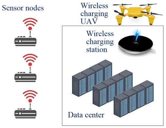
Figure 1. An unmanned data collection system supported by wireless charging of unmanned aerial vehicles.

As shown in Figure 1, the data center is also used as a wireless charging station for the WCUAVs, which travel back and forth between the data center and multiple sensor nodes to collect data when they have sufficient power. The system operates in a frame-based structure [18], where each frame is divided into $S$ transmission slots, with $S < n$. At the start of each frame, each sensor node generates a packet reflecting its current status. This data collection model is common in actual IoT systems, where packets are produced on a regular basis. During a transmission frame, the data center retrieves information from some sensor nodes. At the frame’s conclusion, the data center updates the statuses of the WCUAVs based on the collected information. Furthermore, the sets of sensor nodes associated with different WCUAVs may overlap, meaning that a packet from a single sensor node can be utilized to update multiple WCUAVs.

The three main models are as follows.

• Wireless charging model: The data center is responsible for providing a wireless charging service during each data collection task, ensuring that a WCUAV has sufficient power to complete the tasks. The wireless charging processes between the wireless charging stations and the WCUAVs are considered to be unmanned and reliable. Wireless charging failures are represented by a probabilistic model and an independent Bernoulli distribution, similar to an equipment failure model. This indicates that if WCUAV $m$ is scheduled for wireless charging, the probability of successful wireless charging is denoted by $p_w$. Without loss of generality, the probability is assumed to be quasistatic, meaning its characteristics remain constant over a certain data collection period. It is assumed that the wireless charging failure statistics are not known. The unmanned aerial vehicle that failed to charge can only wait for repair because it was not selected for data transmission.
• Trajectory optimization model: The WCUAVs are responsible for visiting all sensor nodes and collecting data during each task, ensuring that all sensor nodes are visited to transmit data in any given slot. The WCUAV trajectory between the sensor nodes and the data center is considered to be random. Visiting failures and transmission failures are represented by a probabilistic model and an independent Bernoulli distribution, similar to the probabilistic channel model in the traveling salesman problem (TSP). This means that if data from sensor node $r$ is collected by a WCUAV for data transmission, the successful collection probability is denoted by $p_r$. Furthermore, the WCUAV trajectories are assumed to be dynamic, meaning their characteristics remain uncertain over a certain data collection period. It is assumed that the trajectory failure statistics are not known. Any packets remaining on the sensor nodes at each task can only wait, since unvisited sensor nodes were not selected for transmission.
• Age of Information model: The AoI is defined as the time difference between the generation and reception of a data packet (i.e., the current time minus the packet generation time). This indicator emphasizes the freshness of data, rather than the transmission latency in traditional networks. It is assumed that the data center can utilize messages generated simultaneously to refresh the status of a WCUAV.

3.2. Trajectory Performance

The trajectory calculation is based on three main models in Section 3.1, i.e., the wireless charging model, the trajectory optimization model, and the Age of Information model. A typical AoI example with WCUAVs is shown in Figure 2, where there are several consecutive frames, such as $f-1$, $f$, and $f+1$. A WCUAV can fly to a sensor node to collect data or fly to the data center or a charging station for wireless charging.

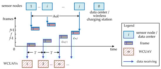
Figure 2. A typical AoI example with WCUAVs.

Figure 2 depicts the typical scenario of AoI for a WCUAV system with a few successive frames sent from different sensor nodes. The period $T$ in Figure 2 measures the transmission time of a data frame from sending to receiving, that is, the frame period from a sensor node to a WCUAV. The AoI in Figure 2 measures the timeliness from data generation to reception and use, i.e., the total time taken for data generation, transmission link delay, and processing at the receiving end. Figure 2 shows the AoI where sensor node 1 starts generating data, and all data from sensor node $j$ is received by WCUAVs. Therefore, the status of WCUAV $m$ will only be updated once the data center has received the most recent packets from all sensor nodes in the frame set $H_m$ of WCUAV $m$ within period $T$, where $H_m=\{1,2,\dots ,f-1$, $f$, $f+1,\dots \}$. The status of this WCUAV is effectively updated at the conclusion of frames. In frame $f$, let $c_{m,f}$ represent the count of frames that have passed since the most recently received packet for WCUAV $m$ was generated. According to Figure 2, the change in $c_{m,f}$ can be formulated as shown in Equation (1).

$$c_{m,f}=\left\{\begin{array}{c}1, if H_m\subseteq H_f\\ c_{m,f-1}+1, otherwise\end{array} \right.,$$

(1)

where $H_f$ denotes the collection of sensor nodes that have their packets successfully delivered within frame $f$.

Let $\lambda (f,t,m) \in \{0,1,\dots ,V\}$ represent the trajectory choice in the $t$th slot of frame $f$ for WCUAV $m$ at slot $t$, where $\lambda (f,t,m) = i$. $i>0$ signifies that sensor node $i$ is selected by WCUAV $m$ for transmission at slot $t$, and $i = 0$ indicates a data center, so no sensor node is selected and the slot remains unused. A trajectory $x$ can be described as a set of trajectory choices, as shown in Equation (2).

$$x={\left\{\lambda \right(f,t,m\left)\right\}}_{f,t,m}.$$

(2)

Let $h(f,t,m)$ signify the AoI for WCUAV $m$ at the commencement of the $t$th slot in frame $f$. Given that updates are permitted solely at the conclusion of a frame, according to Equation (1), it follows that

$$h\left(f,t,m\right)=c_{m,f}T+t-1.$$

(3)

Prior to an update, $h(f,t,m)$ increases steadily with time. Now, the performance of a trajectory $x$ is measured by the anticipated AoI across all WCUAVs within the data collection system, which is represented by Equation (4).

$$g\left(x\right)=\underset{F\to \infty }{\mathit{lim}}sup{\displaystyle \frac{1}{FTM}}{E}^x\left[{\sum }_{f=1}^F{\sum }_{t=1}^T{\sum }_{m=1}^{M}h\left(f,t,m\right)\right].$$

(4)

If all packets necessary to refresh the status of WCUAV $m$ are successfully transmitted within a single frame, for instance, frame $f$, then $h(f+1,t,m)$ will reset to frame period $T$ from $h(f,t,m)$, as all these packets originate at the start of frame $f$. According to Equation (1), AoI performance $g\left(x\right)$ can be rewritten as

$$g\left(x\right)=\underset{F\to \infty }{\mathit{lim}}sup{\displaystyle \frac{T}{FM}}{E}^x\left[{\sum }_{f=1}^F{\sum }_{m=1}^M{c}_{m,f}\right]+{\displaystyle \frac{T-1}{2}}.$$

(5)

In order to simplify analysis and reduce UAV computation, the specified system configuration is considered with $m$ and $T$ as constants. In most practical data collection systems, this situation is reasonable. Then, the optimal strategy to minimize AoI performance $g\left(x\right)$ is the one that attains the minimum $\tilde{g}\left(x\right)$.

$$\tilde{g}\left(x\right)=\underset{F\to \infty }{\mathit{lim}}sup{\displaystyle \frac{1}{F}}{\sum }_{f=1}^F{E}^x\left[{\sum }_{m=1}^M{c}_{m,f}\right].$$

(6)

Our goal is to search for the optimal trajectory $x={\left[\left\{\lambda \left(f,t,m\right)\right\}\right]}_{f,t,m}$ and optimize trajectory performance, leading to a reduced AoI $\tilde{g}\left(x\right)$.

In the absence of sufficient actual statistical and training data, solving this problem is not feasible with deep learning techniques. Motivated by the latest progress in heuristic algorithms, an improved heuristic method may be more suitable for WCUAV trajectory optimization based on UAV edge computing platforms. More specifically, the WCUAV will autonomously make AoI minimization decisions based on a heuristic search policy, with each wireless charging decision being conceptualized as the result of a two-tier decision-making process.

3.3. Energy Constraints

Specifically, the issue to be solved is modeled as a trajectory optimization problem with nonlinear constraints, so the trajectory optimization policy is determined through interactions with the environmental dynamics, such as the successful collection probability $p_r$ and the successful charging probability $p_w$. This proposed approach is well-suited for actual data collection systems where the environment is subject to change, for instance, when $p_r$ or $p_w$ varies gradually. To capitalize on both the spatial and temporal aspects of the AoI minimization problem, multiscale hierarchical nonlinear constraints are created.

It is assumed that there are two sensor nodes or a data center with coordinates $i(x_i,y_i)$ and $j(x_j,y_j)$, and the distance between them can be calculated as a nonlinear constraint in Equation (7).

$$d_{ij}=\sqrt{{(x_i-x_j)}^2+{(y_i-y_j)}^2}.$$

(7)

The distance $d_{ij}$ in Equation (7) can determine the travel time $t_{mij}$ of WCUAV $m$, which means the time it takes for a WCUAV to fly from node $i(x_i,y_i)$ to node $j(x_i,y_i)$. This time is also affected by the flight speed $s_m \left(t\right)$ of WCUAV $m$. Hence, the travel time $t_{mij}$ of WCUAV m can be calculated as follows:

$$t_{mij}=d_{ij}/s_m\left(t\right).$$

(8)

The energy consumption of WCUAV, $e_{mij}$, includes travel energy consumption ($e_{mij}^{travel}$) and wireless communication energy consumption ($e_{mij}^{wlcom}$).

$$e_{mij}=e_{mij}^{travel}+e_{mij}^{wlcom}$$

(9)

The energy consumption $e_{mij}^{travel}$ can be calculated by multiplying the travel time $t_{mij}$ by the flight power $P_{mij}^{flight}$:

$$e_{mij}^{travel}=t_{mij}{P}_{mij}.$$

(10)

The energy consumption of wireless communication ($e_{mij}^{wlcom}$) is closely related to the communication distance, and the two increase exponentially [34]. The mathematical relationship between energy consumption ($e_{mij}^{wlcom}$) and distance ($d_{ij}$) in wireless communication can be expressed as

$$e_{mij}^{wlcom}=\alpha {\left(d_{ij}\right)}^{\beta },$$

(11)

where $\alpha$ is a constant and $\beta$ is the path attenuation index, typically ranging from $2\le \beta \le 4$, depending on the complexity of the environment. For example, in a free space (unobstructed), $\beta =2$, and energy consumption ($e_{mij}^{wlcom}$) is directly proportional to the square of distance ($d_{ij}$). In environments with multiple obstacles, such as urban architectural complexes, $\beta =4$, and energy consumption ($e_{mij}^{wlcom}$) grows faster.

Based on the difference between travel energy consumption ($e_{mij}^{travel}$) and wireless communication energy consumption ($e_{mij}^{wlcom}$), WCUAV $m$ can choose energy conservation methods to plan flight trajectories.

$$\lambda \left(f,t,m\right)=\left\{\begin{array}{c}i,if e_{mij}^{travel}>e_{mij}^{wlcom}\\ j,if e_{mij}^{travel}\le e_{mij}^{wlcom}\end{array}\right..$$

(12)

Assuming the battery capacity of WCUAV $m$ is $e_m^{cap}$, the remaining power $e_m^{bat}$ can be estimated based on energy consumption.

$$e_m^{bat}=e_m^{cap}-{\sum }_i{\sum }_j{e}_{mij}.$$

(13)

Then, we can derive the following series of constraints.

Constraint 1: The energy consumption $e_{mij}$ of WCUAV $m$ is positive and cannot exceed the battery capacity $e_m^{cap}$ of the WCUAV.

$$0<e_{mij}\le e_m^{cap}.$$

(14)

Constraint 2: The remaining power $e_m^{bat}$ of WCUAV $m$ is non-negative and cannot exceed the battery capacity $e_m^{cap}$ of the WCUAV.

$$0\le e_m^{bat}\le e_m^{cap}.$$

(15)

Assuming $P_{mij}^{flight}$ is flight power, $F_{mij}$ is flight force, and $s_m\left(t\right)$ is flight velocity, when flight force and velocity are in the same direction, flight power is equal to the product of flight force and velocity:

$$P_{mij}^{flight}=F_{mij}{s}_m\left(t\right).$$

(16)

Constraint 3: The flight speed $s_m\left(t\right)$ of WCUAV $m$ is non-negative and cannot exceed the maximum flight speed $s_m^{max}$ of the WCUAV.

$$0\le s_m\left(t\right)\le s_m^{max}.$$

(17)

Constraint 4: The flight power $P_{mij}^{flight}$ of WCUAV $m$ is non-negative and cannot exceed the maximum flight power $P_m^{max}$ of the WCUAV.

$$0\le P_{mij}^{flight}\le P_m^{max}.$$

(18)

Assuming $P_{mij}^{charge}$ is wireless charging power and is fixed, wireless charging time $t_m^{charge}$ can be calculated according to the remaining power $e_m^{bat}$ in Equation (13). There is

$$t_m^{charge}={\displaystyle \frac{e_m^{bat}}{P_{mij}^{charge}}}$$

(19)

Considering the successful charging probability $p_w$, Equation (19) can be rewritten as follows:

$$t_m^{charge}=e_m^{bat}/P_{mij}^{charge}/p_w.$$

(20)

Constraint 5: The successful charging probability $p_w$ is non-negative and cannot exceed the maximum value of 1.

$$0\le p_w\le 1.$$

(21)

Constraint 6: The successful collection probability $p_r$ is non-negative and cannot exceed the maximum value of 1.

$$0\le p_r\le 1.$$

(22)

Considering the successful collection probability $p_r$, the total distance $d_m$ of WCUAV $m$ can be calculated according to Equation (7), yielding

$$d_m={\sum }_i{\sum }_j{d}_{ij}/p_r.$$

(23)

Constraint 7: The travel time $t_{mij}$ of WCUAV $m$ is non-negative and limited by the maximum flight speed $s_m^{max}$.

$$0\le d_{ij}/s_m^{max}\le t_{mij}.$$

(24)

The constraints in Equations (25)–(27) limit the trajectory choice $\lambda (f,t,m)$ in the $t$th slot of frame $f$ for WCUAV $m$ to be in the range of $\{0,1,\dots ,V\}$.

Constraint 8: Equation (25) guarantees only one start node, that is, the data center.

$$\lambda (f,t=0,m)=0.$$

(25)

Constraint 9: Equation (26) ensures a continuous path.

$$\lambda \left(f,t+1,m\right)-\lambda \left(f,t,m\right)\ne 0.$$

(26)

Constraint 10: Equation (27) makes sure that there is only one end node or one exit, that is, the data center.

$${\lambda \left(f,t,m\right)|}_{c_{m,f}=1}=0.$$

(27)

The proposed model framework encapsulates the hierarchical nature and wireless charging of the WCUAV trajectory performance, necessitating a large number of nonlinear constraints. However, after careful consideration, the traditional approaches may struggle to produce a satisfactory solution on WCUAV edge computing platforms.

4. An Improved APC Approach

4.1. Algorithm Mechanism

The algorithm mechanism of the APC approach is improved to strengthen its search ability and lower its computing cost.

The improved APC approach for WCUAV trajectory optimization employs three basic operations: seeding, growing, and fruiting. Accordingly, an artificial plant individual can manifest in three forms: a seed, an individual, and a fruit. A seed has a certain probability of growing into an individual or dying, a growing individual has a certain probability of bearing more fruit or dying, and a fruit may grow into a seed or die. These three basic operations endow the APC with three abilities, i.e., global search, fitness comparison, and local search, respectively.

The improved APC approach uses five primary steps to solve the AoI minimization problem: initialization, seeding, growing, fruiting, and end justification.

Step 1. Initialization

The main parameters are initialized, including those of the AoI minimization problem and the APC approach.

The initialization parameters for an AoI minimization problem include $m$ sensor nodes, a data center, a set of WCUAVs, $h(f,t,m)$ of the AoI, $c_{m,f}$ of the frame count, coordinates $i\left(x_i,y_i\right)$, the flight speed $s_m\left(t\right)$, the flight power $P_{mij}^{flight}$, the battery capacity $e_m^{cap}$, the remaining power $e_m^{bat}$, the maximum flight speed $s_m^{max}$, the maximum flight power $P_m^{max}$, the successful charging probability $p_w$, the successful collection probability $p_r$, and the travel time $t_{mij}$.

The initialization parameters for an APC approach include the population size $S$, the seeding probability $p_{seed}$, the growing probability $p_{grow}$, and the fruiting probability $p_{fruit}$. An artificial plant individual is encoded as $x={\left\{\lambda \right(f,t,m\left)\right\}}_{f,t,m}$ in Equation (2). The fitness function $fit$ of APC can select the AoI performance in Equation (4) or the simplified AoI performance in Equation (6).

$$fit=C-g\left(x\right),$$

(28)

where $C$ is a positive constant to obtain a positive fitness value for the AoI minimization problem, and $C>g\left(x\right)$.

Step 2. Seeding

The global search ability is strengthened in the seeding step, where the APC randomly generates seeds in each iteration. The seeding probability $p_{seed}$ ∈ [0,1] decides the global search ability in the whole solution space.

Therefore, the population $\left\{x_{seed}\right(k\left)\right\}$ of the seeds in iteration $k$ includes two parts: random seeds $\left\{x_{seed}^{rand}\left(k\right)\right\}$ for global search with a seeding probability $p_{seed}$, and the fruits ${\{x}_{seed}^{fruit}\left(k-1\right)\}$ in the previous iteration $k-1$ for local search with a probability $(1-p_{seed})$.

$${\left\{x_{seed}\right(k\left)\right\}}_S={\{x_{seed}^{rand}\left(k\right)p_{seed},x_{seed}^{fruit}\left(k-1\right)(1-p_{seed}\left)\right\}}_S.$$

(29)

The population size of seeds in iteration $k$ is $S$. In the first iteration ($k=0$), there is no fruit ($\left\{x_{seed}^{fruit}\left(k-1\right)\right\}=\varnothing$), which means that all seeds $\left\{x_{seed}^{rand}\left(k\right)\right\}$ are randomly produced.

Step 3. Growing

The aim of the growing step is to provide the fittest comparison for the APC approach, where the optimal seeds $\left\{x_{seed}\right(k\left)\right\}$ will be selected with a growing probability $p_{grow}\in [0,1]$. Through the fitness function $fit$ in Equation (28), the population size of the growing individuals $\left\{x_{grow}\right(k\left)\right\}$ will decrease to $S{p}_{grow}$.

$${\{x_{grow}(k)\}}_{S{p}_{grow}}=\{x_{seed}(k)|\underset{S{p}_{\mathit{grow}}}{\max }fit\left(x_{seed}(k)\right){\}}_{S{p}_{grow}}.$$

(30)

Step 4. Fruiting

The local search ability is strengthened in the fruiting step, where the growing individuals $\left\{x_{grow}\right(k\left)\right\}$ will produce more solutions $\left\{x_{fruit}\right(k\left)\right\}$. The population of fruits is composed of the growing individuals $\left\{x_{grow}\right(k\left)\right\}$ with a population size $S{p}_{grow}$, that is, the parthenogenesis of the parent, and the crossing fruits $\left\{x_{fruit}^{cross}\right(k\left)\right\}$ of the parent with a population size $S{p}_{grow}$. Hence, better individuals have more fruiting opportunities, enhancing local search ability. The crossing fruit is determined by a fruiting probability $p_{fruit}\in [0,1]$, which indicates how much original information a parent can retain. Assuming there are two parents, $x_{grow}^a\left(k\right)$ and $x_{grow}^b\left(k\right)$, and they can produce two fruits, we obtain

$$\left\{\begin{array}{c}{x}_{fruit}^{cross}(k)=\{{x_{grow}^a(k)}_{p_{fruit}}//{x_{grow}^b(k)}_{{1-p}_{fruit}}\}\\ x_{fruit}^{cross’}(k)=\{{x_{grow}^b(k)}_{p_{fruit}}//{x_{grow}^a(k)}_{{1-p}_{fruit}}\}\end{array}\right..$$

(31)

where ‘//’ denotes the concatenation of two strings.

Considering two parts of the fruit, namely the parthenogenesis of the parents in Equation (30) and the crossover of the parents in Equation (31), the total population size of the fruits has doubled. There is

$${\{x_{fruit}(k)\}}_{2S{p}_{grow}}=\left\{\{x_{grow}(k){\}}_{S{p}_{grow}},\{x_{fruit}^{cross}(k){\}}_{S{p}_{grow}}\right\}$$

(32)

Step 5. End Justification

The end justification may establish an error threshold $e_{th}$ by the fitness function $fit$ in Equation (28), the maximum number of iterations ${Ite}_{max}$, or the maximum solving period $T_{max}$. If the APC approach detects that any of the end conditions are fit, the iterative calculation is ended and the optimal solution $x^{*}\left(k\right)$ is output. Otherwise, the fruits will be returned to step 2 for the next seeding until the end justification is met.

Figure 3 shows the flowchart of the improved APC approach. There are five primary steps to solve the AoI minimization problem: initialization, seeding, growing, fruiting, and end justification. If the end justification is met, an optimal trajectory $x^{*}\left(k\right)$ can be achieved. Otherwise, the artificial plant community will return and restart the next round of iterative calculations. Figure 3 includes a large loop, which depends on the number of iterations, ${Ite}_{max}$. In each loop, each individual is calculated based on the population size, $S$, and each individual is encoded based on the number of sensors, $n$. It can be seen that the computational complexity of the improved APC approach is $O\left({Ite}_{max}\times S\times n\right)$, where ${Ite}_{max}$ is the maximum number of iterations,$S$ is the population size, and $n$ is the number of sensor nodes.

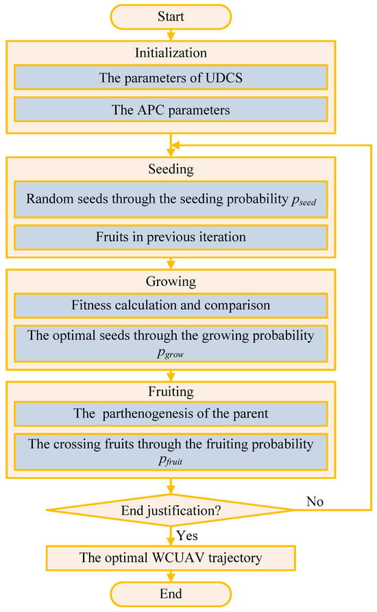
Figure 3. The flowchart of the improved APC approach.

Based on the AoI minimization problem of WCUAVs, two APC approaches are developed in the following two sub-chapters, i.e., the single-WCUAV architecture and the multi-WCUAV architecture.

4.2. Single-WCUAV Architecture

A single-WCUAV architecture is a special scenario involving only one WCUAV, which is also common in real-world data collection activities. Considering the limited computing power of a single WCUAV in this scenario, reducing the computational overhead of the algorithm and extending the operational duration of the WCUAV is of positive significance. For a single-WCUAV architecture, some assumptions are made to simplify the analysis.

First, it is assumed that all sensor nodes and the data center are static, and their positions are fixed in trajectory optimization. All sensor nodes are homogeneous.

Second, the impact of natural disasters and extreme weather is ignored, such as the influence of hurricanes on WCUAV flight, and the impact of extreme high or low temperatures on battery activity.

Third, we assume there are no other UAVs in the work area and that the movements of other UAVs do not affect the flight trajectory and data collection of this WCUAV.

Fourth, we assume that no other UAVs can participate in the collaborative computation of this WCUAV, and no other UAVs can jointly solve the AoI minimization problem during the trajectory optimization period.

According to the four assumptions above, the single-WCUAV architecture algorithm should employ a lightweight mechanism to help us search for the optimal solutions to the AoI minimization problem. On the edge computing platform with limited computing resources and power, the single-WCUAV architecture can be directly deployed. Given $n$ sensor nodes and a data center, the optimal trajectory solution $x^{*}\left(k\right)={\left\{\lambda \right(f,t,m\left)\right\}}_{f,t,m}$ will be calculated through Equation (6). The proposed APC approach utilizes a few parameters and calculation steps to search for the optimal solution, which is NP-hard for traditional techniques to solve. If Equation (6) is met, the system configuration sets $m$ and $T$ as constants, and the optimal trajectory is determined by AoI minimization and wireless charging constants. If Equation (6) is not met, it is not easy for traditional techniques to search for the relaxed constraints where $n$ and $T$ are not constants. To minimize the AoI performance with wireless charging constants, it is recommended to use Equation (4) or (5) when all packets necessary to refresh the status of WCUAV m are successfully transmitted within a single frame.

For the challenges in the single-WCUAV architecture, the improved APC approach in Section 5.1 is introduced here, and the pseudo-code is listed in Algorithm 1. This single-WCUAV architecture strategy decreases computational complexity and makes it easier to meet the AoI minimization requirement with wireless charging constants. This single-WCUAV architecture will search for $x^{*}\left(k\right)={\left\{\lambda \right(f,t,m\left)\right\}}_{f,t,m}$ to include as many sensor nodes as possible, and arrange wireless charging reasonably.

In Algorithm 1, the inputs include $n$ sensor nodes, a data center, a set of WCUAVs, $h(f,t,m)$ o of the AoI, $c_{m,f}$ of the frame count, coordinates $i\left(x_i,y_i\right)$, the flight speed $s_m\left(t\right)$, the flight power $P_{mij}^{flight}$, the battery capacity $e_m^{cap}$, the remaining power $e_m^{bat}$, the maximum flight speed $s_m^{max}$, the maximum flight power $P_m^{max}$, the successful charging probability $p_w$, the successful collection probability $p_r$, and the travel time $t_{mij}$. The initialization parameters for an APC approach include the population size $S$, the seeding probability $p_{seed}$, the growing probability $p_{grow}$, and the fruiting probability $p_{fruit}$.

Algorithm 1. Single-WCUAV architecture

Input: $\{m=1\}$, $\left\{i\right\}$, $h(f,t,m)$, $c_{m,f}$, $\left\{i\left(x_i,y_i\right)\right\}$, $s_m\left(t\right)$, $P_{mij}^{flight}$, $e_m^{cap}$, $e_m^{bat}$, $s_m^{max}$, $P_m^{max}$, $p_w$, $p_r$, and $t_{mij}$.

Constraints: Equations (14), (15), (17), (18), (21), (22), (24)–(27)

Set: $S$, $p_{seed}$, $p_{grow}$, $p_{fruit}$, and $fit$.

Output: The single-WCUAV architecture solution $x^{*}\left(k\right).$

1:   if $n$ and $T$ are constants the n

$\hspace{1em}\hspace{1em}\hspace{1em}fit=C-\mathrm{E}\mathrm{q}\mathrm{u}\mathrm{a}\mathrm{t}\mathrm{i}\mathrm{o}\mathrm{n} \left(6\right)$

2:   else if all packets necessary to refresh the status of WCUAV $m$ are successfully transmitted within a single frame.

$\hspace{1em}\hspace{1em}\hspace{1em}fit=C-\mathrm{E}\mathrm{q}\mathrm{u}\mathrm{a}\mathrm{t}\mathrm{i}\mathrm{o}\mathrm{n} \left(5\right)$

3:   else

$\hspace{1em}\hspace{1em}\hspace{1em}fit=C-\mathrm{E}\mathrm{q}\mathrm{u}\mathrm{a}\mathrm{t}\mathrm{i}\mathrm{o}\mathrm{n} \left(4\right)$

4:   end if

5:   for ${k=1: Ite}_{max}$

6:   $c_{m=1,f+1}=\left\{\begin{array}{c}1, if{H}_{m=1}\subseteq H_f\\ c_{m=1,f}+1, otherwise\end{array} \right.$

7:   $h\left(f,t,m=1\right)=c_{m=1,f}T + t - 1.$

8:   $\left\{x_{seed}^{rand}\left(k\right)\right\}=\mathrm{r}\mathrm{a}\mathrm{n}\mathrm{d}{\left\{\lambda \right(f,t,m=1\left)\right\}}_{f,t,m=1}$

9:   ${\left\{x_{seed}\right(k\left)\right\}}_S={\{x_{seed}^{rand}\left(k\right)p_{seed},x_{seed}^{fruit}\left(k-1\right)(1-p_{seed})\}}_S$

10:   $fit$ calculation

11:   ${\{x_{grow}(k)\}}_{S{p}_{grow}}=\{x_{seed}(k)|\underset{S{p}_{\mathit{grow}}}{\max }fit\left(x_{seed}(k)\right){\}}_{S{p}_{grow}}$

12:   $x_{fruit}^{cross}(k)=\{{x_{grow}^a(k)}_{p_{fruit}}//{x_{grow}^b(k)}_{{1-p}_{fruit}}\}$

13:   ${\{x_{fruit}(k)\}}_{2S{p}_{grow}}=\left\{\{x_{grow}(k){\}}_{S{p}_{grow}},\{x_{fruit}^{cross}(k){\}}_{S{p}_{grow}}\right\}$

14:   $x^{*}\left(k\right)=\left\{\lambda \right(f,t,m=1\left)\right|\mathrm{m}\mathrm{a}\mathrm{x}\left\{fit\right(x\left(k\right)\left)\right\}\}$

15:   if $\left|fit\right(x*\left(k\right))-fit(x*\left(k-1\right)\left)\right|\ge e_{th}$ then return to line 5

16:   end for

17:   Output the optimal solution $x^{*}\left(k\right)$

The constraints include Constraint 1 in Equation (14), Constraint 2 in Equation (15), Constraint 3 in Equation (17), Constraint 4 in Equation (18), Constraint 5 in Equation (21), Constraint 6 in Equation (22), Constraint 7 in Equation (24), Constraint 8 in Equation (25), Constraint 9 in Equation (26), and Constraint 10 in Equation (27). In the optimal solution $x^{*}\left(k\right)$, $\lambda (f,t,m) \in \{0,1,\dots ,V\}$ indicates the trajectory choice in the $t$th slot of frame $f$ for WCUAV $m$, where $\lambda (f,t,m) = i$. $i>0$ signifies that sensor node $i$ is selected by WCUAV $m$ for transmission at slot $t$, and $i = 0$ indicates a data center, so no sensor node is selected and the slot remains unused. Error threshold $e_{th}$ can be predefined by a relative error percentage of the fitness function $fit$ in Equation (28), which is constrained by ten energy constraints. The computational complexity of Algorithm 1 can be calculated as $O\left({Ite}_{max}\times S\times n\right)$, where ${Ite}_{max}$ is the maximum number of iterations,$S$ is the population size, and $n$ is the number of sensor nodes.

4.3. Multi-WCUAV Architecture

If a single WCUAV’s flight status at each time meets the four assumptions in Section 5.2, the single-WCUAV architecture is highly efficient. However, if more WCUAVs are requested to collaborate in executing tasks and the assumptions in Section 5.2 are no longer met, the single-WCUAV architecture may not be applicable for problem-solving. On the one hand, the optimal trajectory solved separately for each WCUAV is not feasible as it may overlap or conflict with the optimal trajectories of other WCUAVs. On the other hand, the integrated solution of the optimal trajectory of multiple WCUAVs needs to integrate their respective edge computing platforms to solve the global optimal solution of all WCUAVs. To address the challenges posed by collaboration and conflict among multiple WCUAVs, a multi-WCUAV architecture is proposed in Algorithm 2, which can be run on the edge computing platforms of multiple WCUAVs to obtain stronger computational power. All WCUAVs are assumed to be homogeneous.

Algorithm 2. Multi-WCUAV architecture

Input: $\{m>1\}$, $\left\{i\right\}$, $h(f,t,m)$, $c_{m,f}$, $\left\{i\left(x_i,y_i\right)\right\}$, $s_m\left(t\right)$, $P_{mij}^{flight}$, $e_m^{cap}$, $e_m^{bat}$, $s_m^{max}$, $P_m^{max}$, $p_w$, $p_r$, and $t_{mij}$.

Constraints: Equations (14), (15), (17), (18), (21), (22), (24)–(27)

Set: $S$, $p_{seed}$, $p_{grow}$, $p_{fruit}$, and $fit$.

Output: The multi-WCUAV architecture solution $x^{*}\left(k\right).$

1:   start communication between $m$ WCUAVs

2:   calculate the total number of WCUAVs

3:   all WCUAVs share inputs

4:   all WCUAVs share constraints

5:   all WCUAVs share APC parameter set

6:   all WCUAVs share outputs

7:   end communication

8:   for ${k=1: Ite}_{max}$

9.   $c_{m,f+1}=\left\{\begin{array}{c}1, if H_m\subseteq H_f\\ c_{m,f}+1, otherwise\end{array} \right.$

10:   $h\left(f,t,m\right)=c_{m,f}T + t - 1.$

11:   $\left\{x_{seed}^{rand}\left(k\right)\right\}=\mathrm{r}\mathrm{a}\mathrm{n}\mathrm{d}{\left\{\lambda \right(f,t,m\left)\right\}}_{f,t,m}$

12:   ${\{x_{seed}(k)\}}_S={\{x_{seed}^{rand}\left(k\right)p_{seed},x_{seed}^{fruit}\left(k-1\right)(1-p_{seed})\}}_S$

13:   $fit$ $=C-Equation \left(6\right)$

14:   ${\{x_{grow}(k)\}}_{S{p}_{grow}}=\{x_{seed}(k)|\underset{S{p}_{\mathit{grow}}}{\max }fit\left(x_{seed}(k)\right){\}}_{S{p}_{grow}}$

15:   $x_{fruit}^{cross}(k)=\{{x_{grow}^a(k)}_{p_{fruit}}//{x_{grow}^b(k)}_{{1-p}_{fruit}}\}$

16:   ${\{x_{fruit}(k)\}}_{2S{p}_{grow}}=\left\{\{x_{grow}(k){\}}_{S{p}_{grow}},\{x_{fruit}^{cross}(k){\}}_{S{p}_{grow}}\right\}$

17:   communication between multiple WCUAVs begins

18:   calculate the fitness on all WCUAVs

19:   compare the fitness on all WCUAVs

20:   $x^{*}\left(k\right)=\left\{\lambda \right(f,t,m=1\left)\right|\mathrm{m}\mathrm{a}\mathrm{x}\left\{fit\right(x\left(k\right)\left)\right\}\}$

21:   end communication

22:   if $\left|fit\right(x*\left(k\right))-fit(x*\left(k-1\right)\left)\right|\ge e_{th}$ then return to line 8

23:   end for

24:   start communication between $m$ WCUAVs

25:   select the optimal solution $x^{*}\left(k\right)$ from all $m$ WCUAVs

26:   end communication

27:   Output the optimal solution $x^{*}\left(k\right)$

The multi-WCUAV architecture is intended to search for the global optimal solution for all WCUAVs. The global assignment of trajectories to all WCUAVs in Algorithm 2 will greatly diminish the overlap or conflict of trajectories of all WCUAVs, which makes it easy to minimize overall AoI. The multi-WCUAV architecture method employs a distributed communication mechanism to fully utilize the edge computing platforms of multiple WCUAVs to obtain a stronger computational power than the single-WCUAV architecture.

The multi-WCUAV architecture for AoI minimization is determined not only by the currently available solution on a single WCUAV but also by the swarm learning of surrounding WCUAVs. Furthermore, the computational power in Algorithm 2 may be affected by the total number of WCUAVs. To overcome the communication overhead, Algorithm 2 diminishes the communication time and computation, making it more suitable for deployment on the edge computing platforms of multiple WCUAVs. Similarly, the error threshold $e_{th}$ can be predefined by a relative error percentage of the fitness function $fit$ in Equation (28), which is constrained by ten energy constraints. Due to the communication required by $m$ WCUAVs during the calculation process, the computational complexity of Algorithm 2 can be obtained as $O\left({Ite}_{max}\times S\times n\times m\right)$, where ${Ite}_{max}$ is the maximum number of iterations,$S$ is the population size, $n$ is the number of sensor nodes, and $m$ is the number of WCUAVs.

5. Benchmark Experiment

In this section, a benchmark test set is designed, and a set of benchmark experiments is carried out through simulations to validate the efficacy of our proposed method.

5.1. Benchmark Test Set

Referring to the IEEE standard for low-rate wireless networks (IEEE Std 802.15.4-2020, Revision of IEEE Std 802.15.4-2015) in [33], we extend the benchmark test set in reference [18], which comprises 19 sensor nodes, to 49 sensor nodes and a data center, i.e., a total of 50 nodes. More than 50 nodes may make the topology structure extremely complex and difficult to read. Consequently, the number of sensor nodes, added WCUAVs, and trajectory optimizations in our AoI minimization challenge is more complex than in [18]. The successful collection probability is set as $p_r\in [0.8,1.0]$ with a uniform distribution, the total number of WCUAVs is 10, and the successful charging probability is set as $p_w \in [0.8,1.0]$, which are not considered in [18]. Unless otherwise specified, each frame period is established at 10 ms. Based on IEEE Std 802.15.4-2020 [33], the detailed benchmark configurations are presented in Table 2.

Table 2. The benchmark configurations.

Benchmark Parameter	Value
The successful collection probability	$p_r \in [0.8,1.0]$
The successful charging probability	$p_w$$\in [0.8,1.0]$
Flight power $P_{mij}^{flight}$	400 w
The maximum flight speed $s_m^{max}$	20 m/s
The battery capacity $e_m^{cap}$	10,000 mAh
Wireless charging power $P_{mij}^{charge}$	50 w
Transfer rate	250 kbps
Frame length	127 bytes
Frame period	10 ms

To measure the performance of the proposed approach, a benchmark data collection map is designed on a square space with horizontal and vertical dimensions of [−1000 m, +1000 m], with positive and negative signs to help observe the flight direction of WCUAVs, as shown in Figure 4. In this benchmark map, 49 sensor nodes are randomly distributed and visited by ten homogeneous WCUAVs, and the data center is located at the center (0.0 m, 0.0 m) and is also the wireless charging station.

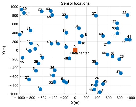
Figure 4. The benchmark map with 49 sensor nodes and a data center.

The benchmark experiments were run on an AMD A6-9225 RADEON R4, a 2.60 GHz CPU, 4.00 GB of RAM, a 64-bit Windows 10 operating system, and MATLAB R2021b simulation software.

In subsequent performance comparison experiments, the improved APC approach was tested and compared with typical baseline approaches, including PSO [1,28], DRL [2,7,22,23,24], GWO [17], ACO [27], and GA [13,28,32]. For the sake of fair comparison, all approaches employed a basic version and the same population size. For the APC algorithm, the population size $S = 1000$, the seeding probability $p_{seed}=0.2$, the growing probability $p_{grow}=0.4$, and the fruiting probability $p_{fruit}=0.7$.

For PSO [1,28], the population size was $S = 1000$, the location limitation was 0.5, the speed limitation was [−0.5, 0.5], the self-learning factor was c1 = 1.5, and the social learning factor was c2 = 1.5. The DRL [2,7,22,23,24] set a state embedding network including a shared stack and multiple heads. This shared stack encompasses two hidden layers, with a batch normalization layer sandwiched between them, where each hidden layer contains 200 neurons activated by the ReLU function. The output from the shared stack is directed towards the head blocks, and each block contains 100 ReLU units followed by |V| + 1 units with tanh activation. The option embedding network mirrors the architecture of the aforementioned shared stack, with the exception that each hidden layer utilizes 100 ReLU units. The tanh function is selected due to its zero-centered nature and its output range being confined between −1 and 1. For GWO [17], the parameters included the population size of gray wolves $S = 1000$, problem dimension dim = 2, and initial positions of the wolf leader (alpha), wolf deputy (beta), and wolf advisor (delta) pos = rand(dim) × 10⁻⁵. The parameters of ACO [27] were set as follows: population size $S = 1000$ ants, the importance of heuristic factors = 5.0, the pheromone volatilization factor = 0.1, and the pheromone importance = 1.0. In the GA [13,28,32], the population size is set to $S = 1000$, the chromosome length to Lind = 20, the crossover probability to $px$ = 0.7, and the mutation probability to pm = 0.01.

5.2. Performance Test

The trajectory curves of a single WCUAV, which collects data from all 49 sensor nodes with one round of wireless charging, are depicted in Figure 5. They are implemented by Algorithm 1, the single-WCUAV architecture. The arrow indicates the flight direction of the WCUAV. Importantly, the proposed APC approach can search for the optimal trajectory to direct the WCUAV to visit a group of sensor nodes with AoI minimization and ultimately return to the data center for wireless charging. In Figure 5, the total trajectory length of the WCUAV is 17,327.16 m, and the AoI value is 432.81 ms. In Figure 5, it is noticeable that the trajectory of WCUAV is too long, which reduces AoI performance, but if the wireless charging frequency increases to reduce the flight range per charge, AoI performance may further deteriorate.

Figure 5. Trajectory of a single WCUAV.

To further improve AoI performance, more WCUAVs are required, which rely on Algorithm 2, the multi-WCUAV architecture. The trajectory maps of 2–10 WCUAVs are shown in Figure 6a–i, where the trajectories of different WCUAVs are shown in different colors. As the number of WCUAVs increases, the proposed APC algorithm can still help WCUAVs search for the optimal trajectory to reduce AoI. When the network nodes and frame period are fixed, more WCUAVs can help improve AoI performance. However, more WCUAVs also necessitate more wireless charging bars, occupying more UAV resources and increasing the total flight range. As shown in Figure 6a, for two WCUAVs, the multi-UAV situation with the lowest number of WCUAVs, the AoI performance has increased compared to a single WCUAV in Figure 5 by 44.161%%, but the total flight range has not increased much, about 12.011%. In the scenario shown in Figure 6i, the maximum number of WCUAVs has reached 10, and the AoI performance has advantages over those of other WCUAVs in Figure 6a–h, but with a maximum flight mileage of 32,517.40 m. Hence, more WCUAVs can provide sufficient time for wireless charging, effectively preventing business failures caused by wireless charging failures.

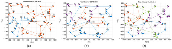
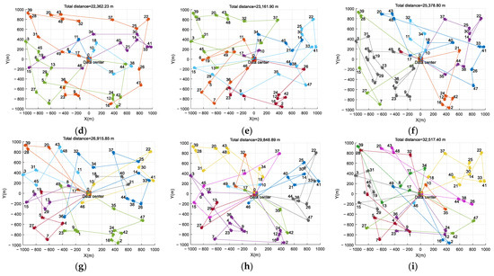
Figure 6. The trajectory maps of 2–10 WCUAVs. (a) m = 2, (b) m = 3, (c) m = 4, (d) m = 5, (e) m = 6, (f) m = 7, (g) m = 8, (h) m = 9, and (i) m = 10 (the trajectories of different WCUAVs are shown in different colors).

Of course, the experimental results in Figure 6a–i can also be used for a single WCUAV traveling back and forth between sensor nodes and wireless charging stations for 2–10 wireless charging cycles. For example, in Figure 6i, a WCUAV needs to make 10 round trips, increasing the total mileage by 87.667%. Considering the duration of each wireless charge and the probability of wireless charging failure, this multiple charging scheme for a single WCUAV significantly degrades AoI performance, and this degradation will intensify with increasing charging times.

Statistical comparisons of the AoI performance for different numbers of WCUAVs are summarized in Table 3. After 20 experiments, with 1–10 WCUAVs each time, the maximum, minimum, and average values, upper limit of 95% confidence interval (95% CI/UL), lower limit of 95% confidence interval (95% CI/LL), and variances of AoI and total flight mileage were calculated. As depicted in Table 3, the proposed APC algorithm performs well in both single-WCUAV and multi-WCUAV scenarios, and can complete optimal trajectory planning with stable solution results, including minimal AoI and total mileage. However, the improvement effect gradually decreases as the number of WCUAVs increases, and the total flight range reaches its maximum value when the number of WCUAVs reaches its maximum value of 10. As indicated in Table 3, the AoI values produced by 10 WCUAVs exhibit more advantages compared to the other nine scenarios. In the 10-WCUAV scenario, the minimum AoI is 92.19 ms and the average AoI is 99.19 ms, realizing 78.470% and 78.641% enhancements in minimum value and average performance in comparison with the single-WCUAV scenario across the wireless charging scenarios. Additionally, two WCUAVs demonstrated the highest cost-effectiveness, with a 44.161% and 45.674% enhancement in minimum and average AoI performance in comparison with the single-WCUAV scenario.

Table 3. Statistics performance comparisons for different numbers of WCUAVs.

		$\mathit{m}=1$	$\mathit{m}=2$	$\mathit{m}=3$	$\mathit{m}=4$	$\mathit{m}=5$	$\mathit{m}=6$	$\mathit{m}=7$	$\mathit{m}=8$	$\mathit{m}=9$	$\mathit{m}=10$
AoI (ms)	max	505.13	278.95	196.53	165.53	140.34	121.10	119.60	112.43	108.00	106.18
	min	428.20	239.11	165.44	147.36	117.84	101.91	102.43	95.20	94.05	92.19
	avg	464.37	252.27	183.94	154.06	127.82	111.84	109.55	103.40	101.36	99.19
	95% CI/UL	473.49	257.80	187.43	155.65	129.74	115.59	110.22	105.31	103.38	101.39
	95% CI/LL	453.40	247.60	179.73	150.32	124.38	110.61	106.39	101.22	99.79	97.76
	variance	525.38	135.34	77.15	37.03	37.45	32.32	19.13	21.82	16.81	17.09
Total distance (m)	max	20,449.99	22,442.10	23,779.58	25,055.94	26,256.50	27,514.87	28,916.48	31,341.73	34,191.26	37,417.18
	min	17,327.16	19,408.38	20,184.98	21,989.92	22,362.23	23,161.90	25,378.80	26,915.85	29,848.89	32,517.40
	avg	18,754.47	20,445.74	22,106.70	23,272.90	24,162.14	25,358.39	26,745.47	29,044.43	31,762.43	34,981.75
	95% CI/UL	19,161.32	20,858.74	22,574.41	23,676.14	24,669.08	25,923.45	27,216.40	29,619.34	32,330.04	35,617.77
	95% CI/LL	18,347.62	20,032.74	21,638.99	22,869.66	23,655.20	24,793.33	26,274.54	28,469.52	31,194.82	34,345.73
	variance	861,754.72	887,994.56	1,138,865.83	846,538.48	1,337,898.21	1,662,276.19	1,154,573.91	1,720,778.97	1,677,342.19	2,106,024.60

5.3. Algorithm Comparisons

This section provides algorithm comparisons, including the improved APC approach, PSO [1,28], DRL [2,7,22,23,24], GWO [17], ACO [27], and GA [13,28,32]. These methods are assessed across the same number of WCUAVs, $m=10$. Subsequently, the sensor nodes affiliated with the selected WCUAV will be scheduled sequentially.

When the network nodes and frame period are fixed, the total distance and the average AoI of six baseline approaches are examined, as shown in Figure 7a,b. The improved APC approach consistently results in the shortest total distance, as shown in Figure 7a, even shorter than that achieved by the DRL approach [2,7,22,23,24]. This is due to the improved APC approach prioritizing WCUAVs with the lowest AoI, with enhanced global search ability and better local search ability compared to the other approaches. When the number of WCUAVs increases from 2 to 10, the APC algorithm has achieved a maximum improvement of 71.096% in total mileage. The DRL [2,7,22,23,24] approach can also obtain good AoI performance, as shown in Figure 7b, meaning that it has a strong learning mechanism, but it is very time-consuming. In this sense, enhanced global search ability and better local search ability of the improved APC approach are crucial for sustaining good AoI performance (Figure 7b), such as multiple WCUAVs with low AoI. However, only adding WCUAVs with the lowest AoI might lead to the waste of some time slots and not significantly enhance the average AoI. As shown in Figure 7a,b, more than ten WCUAVs with the lowest AoI still need information from various sensor nodes, and there are only a few slots left in the current frame. The traditional approaches will struggle to execute the AoI optimization associated with so many WCUAVs, which may not be completed by the frame’s end and will have to be re-executed at the start of the next frame. Compared to other baseline algorithms, the APC algorithm achieves a maximum improvement of 9.791% in the average AoI.

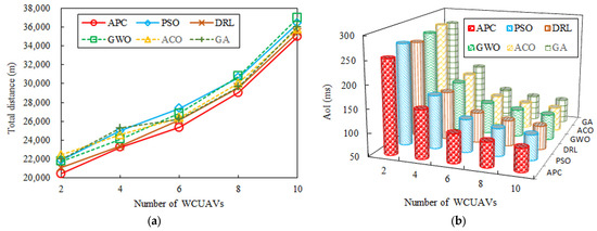
Figure 7. Comparison of baseline approaches versus different numbers of WCUAVs. (a) The total distance. (b) The average AoI.

Figure 8a–c display a comparison of average AoI when the network nodes and frame period are not fixed under the improved APC approach, PSO [1,28], DRL [2,7,22,23,24], GWO [17], ACO [27], and GA [13,28,32].

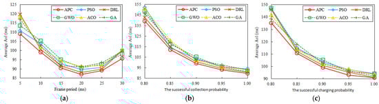
Figure 8. Comparison of average AoI versus different system parameters: (a) versus the frame length T, (b) versus the successful collection probability $p_r$, and (c) versus the successful charging probability $p_w$.

Firstly, for a given data collection system with 50 fixed nodes, there is an optimal frame period $T$ that results in the lowest average AoI. The curve of average AoI changing with frame period can be observed in Figure 8a. With a small $T$, only a limited number of WCUAVs can be updated per frame, leading to a high average AoI. Conversely, when $T$ is considerably large, although more messages can be transmitted within a frame, the waiting time for status updates increases since the data center updates WCUAVs at the frame’s conclusion. When the frame period $T$ is 20, AoI reaches its minimum value, with a decrease of 20.126%. Figure 8a demonstrates that the improved APC approach consistently outperforms the other approaches, with a low average AoI decreased by up to 9.723% and the AoI diminishing as the frame period grows.

Secondly, a highly successful collection probability $p_r$ is helpful to improve AoI performance. The curve of the average AoI changing with the successful collection probability $p_r$ is shown in Figure 8b. Notably, many system states may not maintain consistency with the state space of the original problem, such as the successful collection probability $p_r$. This may result in a dynamic topology with different sensor nodes, leading to changes in the state distribution. This issue is typically solved by fine-tuning the models to match the specific system settings, particularly the exact frame length used in the system. In Figure 8b, when the successful collection probability $p_r$ increases from 0.8 to 1.0, AoI decreases by 35.502%. The APC approach is superior to other algorithms with a maximum improvement of 9.420% because it benefits from the enhanced global search ability in the seeding stage. It is important to remember that the learning seeds for the APC approach are randomly generated in each round to adapt to dynamic changes in the environment.

Thirdly, improving the successful charging probability $p_w$ can help minimize the AoI. Figure 8c shows the curve of the average AoI changing with the successful charging probability $p_w$. Considering the limited power of a WCUAV, wireless charging plays an important role in its trajectory optimization, especially as charging increases. More WCUAVs taking turns working can greatly reduce the impact of wireless charging on AoI, which cannot be achieved by a single WCUAV. In practical systems, if the number of UAVs is limited, it is more plausible and common for successful charging to exceed the successful collection of sensor nodes. In Figure 8c, when the successful charging probability $p_w$ increases from 0.8 to 1.0, AoI decreases by 32.800%. The proposed APC approach can be effectively applied to enhance the system’s information freshness with a maximum improvement of 8.830% over other algorithms because of its better local search ability, where the performance gap between the fruits and the optimal solutions narrows.

Statistical comparisons of the AoI performance on different scenarios of different algorithms are summarized in Table 4, where nine scenarios were considered, i.e., $T=5$, $T=15$, $T=30$, $p_r=0.8$, $p_r=0.9$, $p_r=1.0$, $p_w=0.8$, $p_w=0.9$, and $p_w=1.0$. After 20 experiments, the maximum, minimum, and average values, upper limit of 95% confidence interval (95% CI/UL), lower limit of 95% confidence interval (95% CI/LL), and variances of AoI were calculated. The statistical results show that the proposed APC algorithm has significant improvements compared to other baseline algorithms, with a maximum improvement of 9.768% at the minimum AoI value and 9.733% at the average AoI value.

Table 4. Statistics comparisons for different algorithms.

Scenario	AoI (ms)	APC	PSO	DRL	GWO	ACO	GA
$T=5$	max	115.10	116.78	125.73	119.63	124.53	122.95
	min	103.48	104.82	113.54	107.60	112.47	110.94
	avg	109.03	110.75	119.64	113.53	118.46	116.92
	95% CI/UL	110.77	112.59	121.55	115.39	120.32	118.77
	95% CI/LL	107.29	108.92	117.74	111.68	116.59	115.07
	variance	15.69	17.46	18.86	17.89	18.10	17.82
$T=15$	max	96.51	99.06	97.78	101.22	100.42	97.76
	min	84.49	86.97	85.75	89.17	88.33	85.81
	avg	90.48	92.96	91.70	95.12	94.32	91.72
	95% CI/UL	92.33	94.83	93.56	96.98	96.20	93.55
	95% CI/LL	88.62	91.09	89.85	93.26	92.45	89.89
	variance	17.87	18.22	17.90	18.02	18.28	17.47
$T=30$	max	101.73	106.35	105.95	104.15	106.42	105.73
	min	89.73	94.34	94.02	92.17	94.36	93.68
	avg	95.68	100.34	99.95	98.09	100.34	99.63
	95% CI/UL	97.53	102.18	101.78	99.93	102.21	101.49
	95% CI/LL	93.84	98.49	98.12	96.25	98.48	97.77
	variance	17.72	17.78	17.37	17.62	18.11	18.03
$p_r=0.8$	max	145.06	158.25	148.57	154.77	156.92	152.44
	min	133.10	146.14	136.61	142.76	144.88	140.36
	avg	139.04	152.16	142.53	148.74	150.83	146.35
	95% CI/UL	140.89	154.01	144.36	150.58	152.68	148.22
	95% CI/LL	137.19	150.31	140.70	146.89	148.97	144.48
	variance	17.79	17.87	17.48	17.76	17.99	18.22
$p_r=0.9$	max	106.18	109.75	106.95	111.31	108.05	108.68
	min	92.19	97.74	94.96	99.39	96.10	96.61
	avg	99.19	103.74	100.88	105.30	102.01	102.59
	95% CI/UL	101.39	105.59	102.72	107.12	103.84	104.46
	95% CI/LL	97.76	101.89	99.04	103.48	100.19	100.73
	variance	17.09	17.78	17.67	17.25	17.41	18.15
$p_r=1.0$	max	95.73	99.99	97.00	97.45	99.34	99.01
	min	83.81	88.07	84.95	85.40	87.31	87.03
	avg	89.71	93.98	90.95	91.37	93.28	92.98
	95% CI/UL	91.53	95.80	92.81	93.23	95.13	94.82
	95% CI/LL	87.89	92.16	89.09	89.51	91.43	91.14
	variance	17.26	17.27	18.02	18.04	17.87	17.60
$p_w=0.8$	max	141.26	152.68	152.04	153.27	147.85	144.36
	min	129.26	140.69	140.01	141.26	135.87	132.41
	avg	135.23	146.64	145.95	147.18	141.83	138.34
	95% CI/UL	137.08	148.48	147.81	149.03	143.67	140.17
	95% CI/LL	133.39	144.80	144.10	145.33	139.99	136.51
	variance	17.70	17.64	17.90	17.82	17.62	17.44
$p_w=0.9$	max	106.18	109.75	106.95	111.31	108.05	108.68
	min	92.19	97.74	94.96	99.39	96.10	96.61
	avg	99.19	103.74	100.88	105.30	102.01	102.59
	95% CI/UL	101.39	105.59	102.72	107.12	103.84	104.46
	95% CI/LL	97.76	101.89	99.04	103.48	100.19	100.73
	variance	17.09	17.78	17.67	17.25	17.41	18.15
$p_w=1.0$	max	96.96	100.44	97.30	100.23	99.61	98.41
	min	84.98	88.49	85.27	88.26	87.59	86.43
	avg	90.89	94.39	91.27	94.17	93.54	92.35
	95% CI/UL	92.73	96.22	93.12	96.00	95.39	94.19
	95% CI/LL	89.05	92.56	89.42	92.33	91.69	90.52
	variance	17.61	17.43	17.86	17.55	17.86	17.56

Some suggestions for engineering applications are presented as follows.

Above all, it is recommended to deploy more wireless charging stations on sensor nodes so that WCUAVs can collect data from sensor nodes while implementing wireless charging. In Figure 5, Figure 6, Figure 7 and Figure 8, we only examine a system comprising 1–10 WCUAVs, corresponding to 49 sensor nodes and a wireless charging station. Our benchmark test is not beneficial for the charging operation of WCUAVs, so the average and minimum metrics of the AoI performance are restricted. If more wireless charging stations are built, the AoI can be better than the current experimental results.

Next, according to Figure 5, Figure 6, Figure 7 and Figure 8 and Table 3, more WCUAVs can help improve AoI, but they also increase the cost of UAV usage and make trajectory partitioning more complex. A system comprising 1–10 WCUAVs serves as the benchmark during the experiment phase, where the substantial performance enhancement of the APC approach suggests that the artificial plant individual can extract valuable insights and achieve a reasonably consistent estimation of the trajectory optimization.

Finally, there are the exact limitations in experimental conditions considered for the simulation/emulation. For example, the power consumption of sensor nodes, inter-UAV communication delay, bandwidth constraints, and distributed scheduling overhead are not sufficiently considered here. This manuscript focuses on single objective optimization and AoI minimization, while other objectives are only constraints, such as energy consumption. By considering more WCUAV correlations and more objectives, the above approaches might result in a decrease in AoI performance. Furthermore, if WCUAVs or sensor nodes are not homogeneous, it will exacerbate the decline in solving performance. In this manner, the APC approach is capable of strategically orchestrating trajectory optimization to enhance information freshness, but this requires scalability experiments to verify.

6. Conclusions

In this paper, we have delved into the AoI minimization challenge for unmanned data collection systems with wirelessly charging unmanned aerial vehicles being responsible for data collection from various sensor nodes. By casting the AoI minimization issue as a trajectory optimization problem with a wireless charging policy, we have crafted an improved artificial plant community algorithm to minimize AoI. To improve the adaptability of the algorithm, we provide a single-WCUAV architecture and a multi-WCUAV architecture. The proposed APC approach can generate random seeds in each round to enhance global search ability, and better individuals have more fruiting opportunities to enhance local search ability. The benchmark experiments based on IEEE Std 802.15.4-2020 [33] show that the proposed algorithm can effectively solve challenges and is superior to other algorithms with a maximum improvement of 9.791%. When the number of WCUAVs increased from 1 to 2, the total flight distance increased by 12.011% and the average AoI decreased by 45.674%. When the number of WCUAVs increased from 1 to 10, the total flight distance increased by 87.667% and the average AoI decreased by 78.641%.

Due to limitations in experimental conditions, our work does not consider more metrics or conduct empirical research on actual data collection platforms. Power consumption of sensor nodes, inter-UAV communication delay, bandwidth constraints, and distributed scheduling overhead should be further considered. In the future, considering more factors of WCUAVs in actual UDCSs is a promising direction. An important direction is to validate the scalability and conduct empirical research of the proposed approach on actual WCUAV edge computing hardware or larger sensor networks. Additionally, it is very valuable to integrate and compare more artificial intelligence algorithms and hybrid optimization techniques on WCUAVs.

References

- Wang, P.; Liu, K.; Ma, Y.D.; Gao, Q. AoI and energy-aware data collection for IRS-assisted UAV-IoT networks under jamming. IEEE Internet Things J. 2025, 12, 12166–12180. [Google Scholar] [CrossRef]
- Fu, X.W.; Wang, T.L.; Pace, P.; Aloi, G.; Fortino, G. Low-AoI data collection for UAV-assisted IoT with dynamic geohazard importance levels. IEEE Internet Things J. 2025, 12, 18279–18302. [Google Scholar] [CrossRef]
- Lu, M.X.; Bagheri, M.; James, A.P.; Phung, T. Wireless charging techniques for UAVs: A review, reconceptualization, and extension. IEEE Access 2018, 6, 29865–29884. [Google Scholar] [CrossRef]
- Huang, Z.H.; Chen, H.; Gu, B.; Gong, S.M.; Su, Z.; Guizani, M. A learning-based iterative algorithm for AoI-optimal trajectory planning in UAV-assisted IoT networks. IEEE Trans. Wirel. Commun. 2025, 24, 4598–4613. [Google Scholar] [CrossRef]
- Batista, A.D.; dos Santos, A.L. Resilient UAVs location sharing service based on information freshness and opportunistic deliveries. Pervasive Mob. Comput. 2025, 111, 102066. [Google Scholar] [CrossRef]
- Pei, Y.H.; Zhao, Y.Z.; Hou, F. Minimizing age of information in UAV-assisted edge computing system with multiple transmission modes. Tsinghua Sci. Technol. 2025, 30, 1060–1078. [Google Scholar] [CrossRef]
- Deng, C.; Fu, X.W.; Claudio, S.; Fortino, G. Low-AoI data collection for multi-UAVs-UGVs assisted large-scale IoT systems based on workload balancing. Ad Hoc Netw. 2025, 174, 103844. [Google Scholar] [CrossRef]
- Chen, S.L.; Wei, K.M.; Pei, T.R.; Long, S.Q. AoI-guaranteed UAV crowdsensing: A UGV-assisted deep reinforcement learning approach. Ad Hoc Netw. 2025, 173, 103805. [Google Scholar] [CrossRef]
- Gong, Z.Z.; Hashash, O.; Wang, Y.Z.; Cui, Q.M.; Ni, W.; Saad, W.; Sakaguchi, K. UAV-aided lifelong learning for AoI and energy optimization in nonstationary IoT networks. IEEE Internet Things J. 2024, 11, 39206–39224. [Google Scholar] [CrossRef]
- Xiao, Y.; Lin, Z.J.; Cao, X.X.; Chen, Y.J.; Lu, X.Q. AoI energy-efficient edge caching in AAV-assisted vehicular networks. IEEE Internet Things J. 2025, 12, 6764–6774. [Google Scholar] [CrossRef]
- Li, Y.C.; Ding, H.W.; Yang, Z.J.; Li, B.; Liang, Z.G. Integrated trajectory optimization for UAV-enabled wireless-powered MEC system with joint energy consumption and AoI minimization. Comput. Netw. 2024, 254, 110842. [Google Scholar] [CrossRef]
- Tekin, N. Age of Information minimization for secure data collection in multi-UAV-assisted IoT applications. Internet Things 2025, 33, 101672. [Google Scholar] [CrossRef]
- Gu, Y.; Qiu, H.B.; Chen, B.Q. AoI-minimal task assignment and trajectory optimization in multi-UAV-assisted wireless-powered IoT networks. Drones 2025, 9, 90. [Google Scholar] [CrossRef]
- Wei, Y.K.; Lu, Y.X.; Zhao, P.C.; Leng, S.P.; Yang, K. Minimizing age of information in UAV-assisted data collection with limited charging facilities. IEEE Wirel. Commun. Lett. 2024, 13, 1463–1467. [Google Scholar] [CrossRef]
- Cai, Z.Y.; Yu, Q.Q.; Lu, Z.M.; Liu, Z.Y.; Gong, G.Q. An artificial plant community algorithm for collision-free multi-robot aggregation. Appl. Sci. 2025, 15, 4240. [Google Scholar] [CrossRef]
- Song, F.H.; Yang, Q.X.; Deng, M.S.; Xing, H.L.; Liu, Y.P.; Yu, X.; Li, K.J.; Xu, L.X. AoI and energy tradeoff for aerial-ground collaborative MEC: A multi-objective learning approach. IEEE Trans. Mob. Comput. 2024, 23, 11278–11294. [Google Scholar] [CrossRef]
- Ma, M.F.; Wang, Z.M. Optimizing AoI in IoT networks: UAV-assisted data processing framework integrating cloud-edge computing. Drones 2024, 8, 401. [Google Scholar] [CrossRef]
- Yin, B.; Zhang, S.; Cheng, Y. Application-oriented scheduling for optimizing the age of correlated information: A deep-reinforcement-learning-based approach. IEEE Internet Things J. 2020, 7, 8748–8759. [Google Scholar] [CrossRef]
- Jing, L.L.; Wang, H.; Qin, Z.; Zhu, P. Entropy-based age-aware scheduling strategy for UAV-assisted IoT data transmission. Entropy 2025, 27, 578. [Google Scholar] [CrossRef] [PubMed]
- Lee, J.; So, J. RIS partitioning and UAV selection for age-of-information optimization in RIS-assisted UAV communications. ICT Express 2025, 11, 317–322. [Google Scholar] [CrossRef]
- Zeng, R.; Luo, R.; Liu, B. UAV path planning for forest firefighting using optimized multi-objective jellyfish search algorithm. Mathematics 2025, 13, 2745. [Google Scholar] [CrossRef]
- Liu, Y.X.; Deng, Q.Y.; Zeng, Z.W.; Liu, A.F.; Li, Z.T. A hybrid optimization framework for age of information minimization in UAV-assisted MCS. IEEE Trans. Serv. Comput. 2025, 18, 527–542. [Google Scholar] [CrossRef]
- Zhou, X.H.; Xiong, J.; Zhao, H.T.; Yan, C.; Wang, H.J.; Wei, J.B. Population-invariant MADRL for AoI-aware UAV trajectory design and communication scheduling in wireless sensor networks. IEEE Internet Things J. 2025, 12, 2545–2561. [Google Scholar] [CrossRef]
- He, Y.; Hu, R.; Liang, K.; Liu, Y.; Zhou, Z. Deep reinforcement learning algorithm with long short-term memory network for optimizing unmanned aerial vehicle information transmission. Mathematics 2025, 13, 46. [Google Scholar] [CrossRef]
- Pan, J.N.; Li, Y.; Chai, R.; Xia, S.C.; Zuo, L.L. Age of information aware trajectory planning of UAV. IEEE Trans. Cogn. Commun. Netw. 2024, 10, 2344–2356. [Google Scholar] [CrossRef]
- Liu, X.Y.; Liu, H.H.; Zheng, K.C.; Liu, J.; Taleb, T.; Shiratori, N. AoI-minimal clustering, transmission and trajectory co-design for UAV-assisted WPCNs. IEEE Trans. Veh. Technol. 2025, 74, 1035–1051. [Google Scholar] [CrossRef]
- Zhou, X.Y.; Zhu, Q. Optimization algorithm for AoI-based UAV-assisted data collection. Int. J. Distrib. Sens. Netw. 2024, 2024, 6691579. [Google Scholar] [CrossRef]
- Wang, D.W.; Yuan, L.F.; Pang, L.N.; Xu, Q.; He, Y.X. Age of information-inspired data collection and secure upload assisted by the unmanned aerial vehicle and reconfigurable intelligent surface in maritime wireless sensor networks. Drones 2024, 8, 267. [Google Scholar] [CrossRef]
- Cai, Z.; Ma, Z.; Zuo, Z.; Xiang, Y.; Wang, M. An image edge detection algorithm based on an artificial plant community. Appl. Sci. 2023, 13, 4159. [Google Scholar] [CrossRef]
- Cai, Z.Y.; Jiang, S.; Dong, J.H.Z.; Tang, S.J. An artificial plant community algorithm for the accurate range-free positioning of wireless sensor networks. Sensors 2023, 23, 2804. [Google Scholar] [CrossRef]
- Xie, C.; Wu, B.B.; Pan, Z.H.; Guo, D.X.; Ma, W.F. AoI-optimal path planning for UAV-assisted data collection with heterogeneous information aging speed. IET Commun. 2025, 19, e12768. [Google Scholar] [CrossRef]
- Zhao, M.X.; Xiao, Y.M.; Yao, J.P.; Wang, T.D.; Lee, J.; Quek, T.Q.S. Up-downlink AoI-driven multi-source data collection in UAV-assisted wireless sensor networks. IEEE Trans. Wirel. Commun. 2025, 24, 1178–1192. [Google Scholar] [CrossRef]
- IEEE Std 802.15.4-2020; IEEE Standard for Low-Rate Wireless Networks (Revision of IEEE Std 802.15.4-2015). IEEE Computer Society: Washington, DC, USA, 2020. [CrossRef]
- Kanellopoulos, D.; Sharma, V.K. Survey on power-aware optimization solutions for MANETs. Electronics 2020, 9, 1129. [Google Scholar] [CrossRef]
Disclaimer/Publisher’s Note: The statements, opinions and data contained in all publications are solely those of the individual author(s) and contributor(s) and not of MDPI and/or the editor(s). MDPI and/or the editor(s) disclaim responsibility for any injury to people or property resulting from any ideas, methods, instructions or products referred to in the content. |
© 2025 by the authors. Licensee MDPI, Basel, Switzerland. This article is an open access article distributed under the terms and conditions of the Creative Commons Attribution (CC BY) license (https://creativecommons.org/licenses/by/4.0/).