Long-Term Behavior of Lotka–Volterra Model with Lévy Jump in Countable State-Dependent Environments

Abstract

In this study, we analyze a multi-species mutualistic Lotka–Volterra model with Lévy jumps and regime-switching. A defining feature of the work lies in modeling the random environment through state-dependent switching in an infinite countable state space. Our main objective is to establish the sufficient conditions of the extinction and stochastic permanence of the model. First, we analyze the existence and uniqueness of the model’s solution, followed by an examination of the solution’s stochastic ultimate boundedness. Moreover, the challenges arising from state-dependent switching are addressed using the stochastic comparison method. Due to the presence of the jump component, more complex conditions are required to achieve a finite partition of the countably infinite space. Furthermore, the M-matrix theory is also used to obtain the stochastic permanence property. Finally, two specific examples are provided to illustrate the conclusions in this paper.

1. Introduction

The classical Lotka–Volterra model, since its independent formulation by Alfred Lotka [1] and Vito Volterra [2] in the early 20th century, has served as the cornerstone of quantitative ecology by mathematically describing species interactions such as predation, competition, and mutualism. However, this deterministic framework inherently assumes constant environmental conditions and linear interaction rules, failing to capture the episodic, state-dependent perturbations that characterize real-world ecosystems—from seasonal resource fluctuations to abrupt climate shifts or human-induced disturbances. While early stochastic extensions addressed this gap by incorporating continuous noise (e.g., Brownian motion, see ref. [3,4,5,6]), they remained limited in modeling discrete, regime-like changes in environmental states, where system parameters undergo sudden transitions rather than gradual fluctuations. This limitation spurred the development of the regime-switching Lotka–Volterra model, a hybrid framework that integrates the nonlinear dynamics of species interactions with the discrete state transitions of a continuous-time Markov chain or state-dependent switching, enabling more realistic representations of ecosystems and other complex systems operating under heterogeneous conditions. For a comprehensive exploration of switching diffusions, please refer to ref. [7].

The conceptual foundation of state-dependent switching Lotka–Volterra models lies in their ability to encode regime changes as responses to predefined thresholds of the system’s internal state variables. Each regime is associated with distinct parameter values governing species growth, interaction, and mortality rates, and transitions between regimes occur when key state variables (e.g., prey population size, competitor density) cross critical thresholds. For instance, an ecosystem might shift from a “low-competition” regime (moderate growth rates, weak interspecific interference) to a “high-competition” regime (suppressed growth rates, intense resource rivalry) when the total community biomass exceeds a threshold, or a predator–prey system could transition from “active predation” to “scavenging” when prey density drops below a survival threshold. This hybrid structure addresses a critical shortcoming of deterministic, continuous-stochastic, and even Markov-switching Lotka–Volterra models: the inability to replicate phenomena where regime shifts are not random but are direct consequences of the system’s own dynamics, such as Allee effects triggering population collapse or density-dependent foraging strategies altering interaction strengths.

Early theoretical advancements, such as the analysis of Markov switching Lotka–Volterra models, laid the mathematical groundwork for understanding the model’s key properties, including solution existence, uniqueness, and threshold-induced behaviors like hysteresis or sudden regime shifts, by leveraging piecewise-smooth dynamical systems and invariant manifold theory; see ref. [8,9,10,11,12,13] and so on. For example, Wu et al. [14] investigated a stochastic Lotka–Volterra model driven by Lévy jumps with Markov switching, obtaining sufficient conditions for stochastic permanence and extinction. Moreover, the state-dependent switching, which arises from the interplay between discrete switching and continuous diffusion processes, also demonstrates strong applicability. Basak et al. [15] discussed the ergodicity of diffusion processes under state-dependent switching. In their research, Shao [16] derived conditions guaranteeing the existence and uniqueness of invariant measures for diffusion processes under state-dependent switching. Furthermore, numerical algorithms were constructed, and the rates of convergence for these algorithms were provided. Ji et al. [17] studied properties such as the existence of stationary distributions for stochastic Lotka–Volterra models under state-dependent switching. While recent works on the Lotka–Volterra model predominantly focus on finite state space regime-switching, considering multiple factors naturally leads to the exploration of state-dependent regime-switching with a countable state space, which is the main focus of this study.

In this paper, we consider the following stochastic Lotka–Volterra system:

$$\begin{array}{cc}\hfill \mathrm{d}x\left(t\right)=\mathrm{diag}(x_1\left(t\right),\dots ,x_n\left(t\right))& (\left(b\left(r\right(t\left)\right)+A\left(r\right(t\left)\right)x\left(t\right)\right)\mathrm{d}t\hfill \\ & +\sigma \left(r\left(t\right)\right)\mathrm{d}B\left(t\right)+{\int }_{{\mathbb{R}}_0}D(r\left(t\right),z)\tilde{N}(\mathrm{d}t,\mathrm{d}z)),\hfill \end{array}$$

(1)

where $x={(x_1,\dots ,x_n)}^T\in {\mathbb{R}}^n$ represents the population size; and $\left\{r\right(t),t⩾0\}$ takes values in $\mathcal{S}=\{1,2,\dots ,\infty \},$ which is a state-dependent switching process with the generator $Q\left(x\right)$ given by:

$$\begin{array}{c}\hfill P\{r(t+\mathsf{\Delta })=l\mid r\left(t\right)=k,x\left(t\right)=x\}=\left\{\begin{array}{cc}{q}_{kl}\left(x\right)\mathsf{\Delta }+o\left(\mathsf{\Delta }\right),\hfill & \mathrm{if}l\ne k,\hfill \\ 1+q_{kk}\left(x\right)\mathsf{\Delta }+o\left(\mathsf{\Delta }\right),\hfill & \mathrm{if}l=k,\hfill \end{array}\right.\end{array}$$

(2)

where $\mathsf{\Delta }\downarrow 0,\forall k,l\in \mathcal{S}.$ For any $k\in \mathcal{S}$, $b\left(k\right)={(b_1\left(k\right),\dots ,b_n\left(k\right))}^T\in {\mathbb{R}}^n$ denotes the net growth rate of the population in the kth state; $A\left(k\right)={\left(a_{ij}\left(k\right)\right)}_{n\times n}\in {\mathbb{R}}^{n\times n}$ represents the intensity of interactions between species in the kth state; $\sigma \left(k\right)={\left({\sigma }_{ij}\left(k\right)\right)}_{n\times n}\in {\mathbb{R}}^{n\times n}$ denotes the noise intensity in the kth state; $B\left(t\right)={(B_1\left(t\right),\dots ,B_n\left(t\right))}^T$ is an n-dimensional standard Brownian motion; $D(k,z)={(D_1(k,z),\dots ,D_n(k,z))}^T:\mathcal{S}\times {\mathbb{R}}_0\to {\mathbb{R}}^n$ represents the jump amplitude in the kth state; $\tilde{N}(\mathrm{d}t,\mathrm{d}z)=N(\mathrm{d}t,\mathrm{d}z)-\nu \left(\mathrm{d}z\right)\mathrm{d}t$ is the compensated Poisson random measure, where $N(\mathrm{d}t,\mathrm{d}z)$ is a Poisson random measure with intensity $\mathrm{d}t·\nu \left(\mathrm{d}z\right)$, and $\nu \left(\mathrm{d}z\right)$ is a $\sigma$-finite measure satisfying ${\int }_{{\mathbb{R}}_0}{(1\wedge |z|}^2)\nu \left(\mathrm{d}z\right)<\infty ,$ with ${\mathbb{R}}_0=\mathbb{R}\setminus \left\{0\right\}$. Assume that $b_i\left(k\right)>0$, $a_{ij}\left(k\right)>0$ ($i\ne j$), and $a_{ii}\left(k\right)<0$, for all $k\in \mathcal{S}$, $i=1,\dots ,n$. This implies that the interactions between species are mutualistic. Moreover, the Brownian motion $B\left(t\right)$, the switching process $r\left(t\right)$, and the Poisson random measure $N(\mathrm{d}t,\mathrm{d}z)$ are mutually independent. We take the initial values $x\left(0\right)=x_0$ and $r\left(0\right)=k_0$.

For $\left(x\right(t),r(t\left)\right)$, the generator $\mathcal{A}$ is as follows (see [Chapter 2] [7]). For any function $V:{\mathbb{R}}^n\times \mathcal{S}\mapsto {\mathbb{R}}_{+}$ with $V(·,k)\in C^2\left({\mathbb{R}}^n\right)$ for each $k\in \mathcal{S}$, we define

$$\begin{array}{c}\hfill \mathcal{A}V(x,k,t)={\displaystyle \frac{\partial V(x,k,t)}{\partial t}}+{\mathcal{L}}^{\left(k\right)}V(x,k,t)+Q\left(x\right)V(x,k,t),\end{array}$$

where

$$\begin{array}{cc}\hfill {\mathcal{L}}^{\left(k\right)}V(x,k,t)& =〈\nabla V(x,k,t),\mathrm{diag}\{x_1,\dots ,x_n\}(b\left(k\right)+A\left(k\right)x)〉\hfill \\ & +{\displaystyle \frac{1}{2}}\mathrm{tr}\left({\sigma }^T\left(k\right)\mathrm{diag}\{x_1^2,\dots ,x_n^2\}\sigma \left(k\right){\nabla }^{2}V(x,k)\right)\hfill \\ \hfill & +{\int }_{{\mathbb{R}}_0}(V(x+\mathrm{diag}\{x_1,\dots ,x_n\}D(k,z),k,t)-V(x,k,t)\hfill \\ & -〈\nabla V(x,k,t),\mathrm{diag}\{x_1,\dots ,x_n\}D(k,z)〉)\nu \left(\mathrm{d}z\right),\hfill \\ \hfill Q\left(x\right)V(x,k,t)& =\sum _{l\in \mathcal{S}}{q}_{kl}\left(x\right)V(x,l,t).\hfill \end{array}$$

Here and hereafter, $\nabla V(·,k,t)$ denotes the gradient of $V(·,k,t)$, while ${\nabla }^{2}V(·,k,t)$ denotes the Hessian matrix of $V(·,k,t)$. $\langle A,B\rangle$ shows the inner product of vectors A and B.

One of our main aims here is to establish the sufficient conditions of the extinction and stochastic permanence for systems (1) and (2). However, there are the inherent challenges for the state-dependent switching process in a countable space. Firstly, the state-dependent switching process fails to satisfy the ergodic property of Markov chains, which increases the difficulty of analyzing its long-term behavior. Secondly, the presence of a countable state space renders M-matrix theory ineffective for the study of stochastic permanence. To solve the difficulties above, we introduce the methods of stochastic comparison theorems for state-dependent switching and finite partition for an infinitely countable state space. These ideas have been employed extensively across various studies. For instance, by applying the weak Harris theorem, ref. [18] employed this idea to analyze the exponential ergodicity (in the Wasserstein distance) of birth–death-type state-dependent switching diffusion processes. Meanwhile, ref. [19] constructed a comparison theorem for more general state-dependent switching diffusion processes—aiming to discard the birth–death-type switching restriction and extend applicability to processes with an infinitely countable state space. Xi et al. [20], in turn, examined the existence and uniqueness of strong solutions, the strong Feller property, and exponential ergodicity for jump-diffusion processes with countable state space switching. However, few authors have studied biological models with state-dependent switching in a countably infinite space. To the best of the authors’ knowledge, Bui and Yin [21] studied the persistence and extinction of two-time-scale Lotka–Volterra models under Markov switching in countable state spaces. Additionally, Bao and Shao [22] developed a criterion to assess the extinction of infectious individuals for a range of random/stochastic SIRS models featuring state-dependent switching within a finite state space.

The core innovations and contributions of this paper are reflected in two aspects: first, for the first time, we introduce the mechanism of countably infinite state-dependent switching into the classical Lotka–Volterra model, breaking through the finiteness constraint on switching settings in traditional models and better conforming to the dynamic characteristics of complex ecosystems; second, centered on this extended model, we systematically analyze the long-time behavior of species competition, accurately depict the laws of species dynamic evolution, and establish key benchmarks for determining their permanent persistence or eventual extinction. This innovation not only provides a more practical theoretical framework for the research of complex ecosystems but also transforms the original complex model with countably infinite discrete states into an efficient analytical tool by constructing a tractable reduced diffusion system. When addressing the core issue of the persistence or extinction of competing species, it significantly reduces computational complexity and offers a more practical research pathway for in-depth exploration of related ecological problems.

The organization of this paper is as follows: In Section 2, we study existence, uniqueness, and stochastic ultimate boundedness of the Lotka–Volterra systems associated with a regime-switching with a countable state space. We then introduce the stochastic comparison approach to obtain the extinction of the Lotka–Volterra systems in Section 3. Section 4 provides the stochastic permanence of the systems with the method of the finite partition in a countable space. Finally, two specific examples are provided to illustrate the conclusions in this paper.

2. Preliminaries

Throughout this paper, let $(\mathsf{\Omega },\mathcal{F},{\left({\mathcal{F}}_t\right)}_{t⩾0},\mathbb{P})$ be a complete filtered probability space satisfying the usual conditions. The stochastic processes studied in this work are all defined on this filtered probability space. This section shows the existence and uniqueness of the global positive solution to the system (1) and (2). The stochastic ultimate boundedness of the model is also provided.

2.1. Existence and Uniqueness of Positive Solution

It is first necessary to prove that the system (1) and (2) admits a global positive solution. For this purpose, the following assumptions are made:

(A1)

For all $k\in \mathcal{S}$, $i=1,2,\dots ,n$, $z\in {\mathbb{R}}_0$, $D_i(k,z)>-1$, and there exists a positive constant $K>0$ such that

$${\int }_{{\mathbb{R}}_0}[D_i(k,z)-log(1+D_i(k,z))]\nu \left(\mathrm{d}z\right)⩽K,\mathrm{and}{\int }_{{\mathbb{R}}_0}{D}_i^2(k,z)\nu \left(\mathrm{d}z\right)<\infty .$$

(A2)

The matrix $Q\left(x\right)={\left(q_{kl}\left(x\right)\right)}_{k,l\in \mathcal{S}}$ is irreducible and conservative, i.e., $q_{kk}\left(x\right)=-{\displaystyle \sum _{l\in \mathcal{S},l\ne k}}{q}_{kl}\left(x\right)$, and

$$M:=\underset{k\in \mathcal{S}}{sup}\underset{x\in {\mathbb{R}}^n}{sup}(-q_{kk}\left(x\right))<\infty .$$

Remark 1.

In natural ecosystems, population size fluctuations consistently occur within a “feasible interval” (i.e., $D_i(k,z)>0$). The condition that $D_i(k,z)>-1$ acts as a mathematical constraint for this interval, which biologically corresponds to the “minimum resilience of populations to withstand disturbances” and precludes the model from generating biologically implausible results such as “negative population size.”

Theorem 1.

Suppose conditions (A1)–(A2) hold. For any $k\in \mathcal{S}$, assume that there exist some positive constants $c_1\left(k\right),\dots ,c_n\left(k\right)$ such that

$$-\lambda :=\underset{k\in \mathcal{S}}{sup}\left\{{\lambda }_{max}^{+}\left(\overline{C}\left(k\right)A\left(k\right)+A^T\left(k\right)\overline{C}\left(k\right)\right)\right\}⩽0,$$

where $\overline{C}\left(k\right)=\mathrm{diag}(c_1\left(k\right),\dots ,c_n\left(k\right)).$ Then, for any initial value $x_0\in {\mathbb{R}}_{+}^n$, $k_0\in \mathcal{S}$, the system (1) and (2) almost surely admits a unique global positive solution.

Proof. 

Given that the coefficients of Equation (1) satisfy local Lipschitz continuity, we can infer from [Theorem A.2] [12] that for any prescribed initial value $x_0\in {\mathbb{R}}_{+}^n$, a unique local solution $x\left(t\right)\in {\mathbb{R}}_{+}^n$ exists on the interval $t\in [0,{\zeta }_e)$, where ${\zeta }_e$ denotes the explosion time. Our task thus reduces to proving that the solution is non-explosive. Now, we prove ${\zeta }_e=\infty ,a.s.$ Let $m_0⩾1$ be sufficiently large such that $x_0$ lies within the interval $[{\displaystyle \frac{1}{m_0}},m_0]$. For each integer $m⩾m_0$, define the stopping time:

$$\begin{array}{c}\hfill {\zeta }_m:=inf\{t\in (0,{\zeta }_e):x\left(t\right)⩽{\displaystyle \frac{1}{m}}\mathrm{or}x\left(t\right)⩾m\},\end{array}$$

where throughout this paper, we set $inf⌀=\infty$. Obviously, ${\zeta }_m$ is increasing as $m\to \infty$. Set ${\zeta }_{\infty }={lim}_{m\to \infty }{\zeta }_m$, whence ${\zeta }_{\infty }⩽{\zeta }_e,a.s.$ That is to say, to complete the proof, we only need to show ${\zeta }_{\infty }=\infty ,a.s.$ If this assertion is not true, then there is a pair of constants $T>0$ and $ϵ\in (0,1)$ such that

$$\begin{array}{c}\hfill \mathbb{P}\{{\zeta }_{\infty }⩽T\}⩾ϵ.\end{array}$$

(3)

Therefore, there exists an integer $m_1⩾m_0$ such that

$$\begin{array}{c}\hfill \mathbb{P}\{{\zeta }_m⩽T\}⩾ϵ\mathrm{for}\mathrm{any}m⩾m_1.\end{array}$$

In addition, define the function V:

$$V(x,k)=C\left(k\right)[x-\mathbf{1}-logx],$$

where $C\left(k\right)=(c_1\left(k\right),\dots ,c_n\left(k\right))$, and $\mathbf{1}={(1,\dots ,1)}^T$. The following can be computed:

$$\begin{array}{cc}\hfill \mathcal{A}V(x,k)& ={\mathcal{L}}^{\left(k\right)}V(x,k)+Q\left(x\right)V(x,k)\hfill \\ \hfill & =x^T\overline{C}\left(k\right)b\left(k\right)+x^T\overline{C}\left(k\right)A\left(k\right)x-C\left(k\right)(b\left(k\right)+A\left(k\right)x)\hfill \\ \hfill & +{\displaystyle \frac{1}{2}}{\sigma }^T\left(k\right)\overline{C}\left(k\right)\sigma \left(k\right)+\sum _{i=1}^n{c}_i\left(k\right){\int }_{{\mathbb{R}}_0}\left[D_i(k,z)-log\left(1+D_i(k,z)\right)\right]\nu \left(\mathrm{d}z\right)\hfill \\ \hfill & +\sum _{l=1}^{\infty }{q}_{kl}\left(x\right)V(x,l).\hfill \end{array}$$

(4)

By $-\lambda :=\underset{k\in S}{sup}\left\{{\lambda }_{max}^{+}(\overline{C}\left(k\right)A\left(k\right)+A^T\left(k\right)\overline{C}\left(k\right))\right\}⩽0$, we get

$$x^T\overline{C}\left(k\right)A\left(k\right)x={\displaystyle \frac{1}{2}}{x}^T(\overline{C}\left(k\right)A\left(k\right)+A^T\left(k\right)\overline{C}\left(k\right))x⩽{\displaystyle \frac{-\lambda }{2}}{\left|x\right|}^2.$$

Furthermore, for any $k\in \mathcal{S}$, it holds from (A1) that

$$\begin{array}{cc}\hfill {\mathcal{L}}^{\left(k\right)}V(x,k)& ⩽{\displaystyle \frac{-\lambda }{2}}{\left|x\right|}^2+\sum _{i=1}^n{c}_i\left(k\right)\left(b_i\left(k\right)-a_{ii}\left(k\right)\right)x_i+{\displaystyle \frac{1}{2}}{\sigma }^T\left(k\right)\overline{C}\left(k\right)\sigma \left(k\right)-C\left(k\right)b\left(k\right)\hfill \\ \hfill & +\sum _{i=1}^n{c}_i\left(k\right){\int }_{{\mathbb{R}}_0}\left[D_i(k,z)-log\left(1+D_i(k,z)\right)\right]\nu \left(\mathrm{d}z\right)\hfill \\ \hfill & ⩽{\displaystyle \frac{-\lambda }{2}}{\left|x\right|}^2+\sum _{i=1}^n{c}_i\left(k\right)\left(b_i\left(k\right)-a_{ii}\left(k\right)\right)x_i+{\displaystyle \frac{1}{2}}{\sigma }^T\left(k\right)\overline{C}\left(k\right)\sigma \left(k\right)+\sum _{i=1}^n{c}_i\left(k\right)(K-b\left(k\right)).\hfill \end{array}$$

Therefore, there exists a constant $K_1>0$ such that

$$\begin{array}{c}\hfill {\mathcal{L}}^{\left(k\right)}V(x,k)⩽K_1.\end{array}$$

(5)

For $k,l\in \mathcal{S}$, let $K_2=sup\left\{{\displaystyle \frac{c_i\left(l\right)}{c_i\left(k\right)}}:1⩽i⩽n,k,l\in \mathcal{S}\right\}$. According to the definition of V, we have

$$\begin{array}{cc}\hfill V(x,l)=& C\left(l\right)[x-1-logx]=\sum _{i=1}^n{c}_i\left(l\right)[x_i-1-log\left(x_i\right)]\hfill \\ \hfill ⩽& \sum _{i=1}^n{K}_2{c}_i\left(k\right)[x_i-1-log\left(x_i\right)]=K_{2}V(x,k),\hfill \end{array}$$

Then,

$$\begin{array}{cc}\hfill Q\left(x\right)V(x,k)& =\sum _{l=1}^{\infty }{q}_{kl}\left(x\right)V(x,l)⩽K_2\left(\sum _{l=1}^{\infty }\left|q_{kl}\left(x\right)\right|\right)V(x,k)\hfill \\ \hfill & =2K_2(-q_{kk}\left(x\right))V(x,k)⩽2K_{2}MV(x,k).\hfill \end{array}$$

(6)

Therefore, substituting (5) and (6) into (4), there exists a constant $K_3>0$ such that

$$\mathcal{A}V(x,k)⩽K_3[1+V(x,k)].$$

By the generalized Itô formula, for any $t\in [0,T]$, we have

$$\begin{array}{cc}\hfill \mathbb{E}V(x(t\wedge {\zeta }_m),r(t\wedge {\zeta }_m))& =V(x_0,k_0)+\mathbb{E}{\int }_0^{t\wedge {\zeta }_m}\mathcal{A}V(x\left(s\right),r\left(s\right))\mathrm{d}s\hfill \\ \hfill & ⩽V(x_0,k_0)+\mathbb{E}{\int }_0^{t\wedge {\zeta }_m}{K}_3(1+V(x\left(s\right),r\left(s\right)))\mathrm{d}s\hfill \\ \hfill & ⩽K_4+K_3{\int }_0^T\mathbb{E}V(x(s\wedge {\zeta }_m),r(s\wedge {\zeta }_m))\mathrm{d}s,\hfill \end{array}$$

where $K_4=V(x_0,k_0)+K_{3}T$. By Gronwall’s inequality, we obtain

$$\begin{array}{c}\hfill \mathbb{E}V(x(T\wedge {\zeta }_m),r(T\wedge {\zeta }_m))⩽K_4{e}^{K_{3}T}.\end{array}$$

(7)

For $m⩾m_1$, let ${\mathsf{\Omega }}_m=\{{\zeta }_m⩽T\}$. From (3), it follows that $\mathbb{P}\left({\mathsf{\Omega }}_m\right)⩾\epsilon$. Note that for every $\omega \in {\mathsf{\Omega }}_m$, there exists some i such that $x_i({\zeta }_m,\omega )$ equals either m or $1/m$. Therefore, $V(x({\zeta }_m,\omega ),k)$ is no less than

$$C\left(k\right)[m-1-log(m\left)\right]\mathrm{or}C\left(k\right)[1/m-1-log(1/m\left)\right].$$

Then,

$$\mathbb{E}\left[V(x(t\wedge {\zeta }_m),r(t\wedge {\zeta }_m))\right]⩾C\left(k\right)[(m-1-log\left(m\right))\wedge (1/m-1-log(1/m))],\omega \in {\mathsf{\Omega }}_m.$$

Letting $m\to \infty$, we derive a contradiction from (7):

$$\infty =\mathbb{E}V(x({\zeta }_m,\omega ),r({\zeta }_m,\omega ))⩽K_4{e}^{K_{3}T}.$$

Thus, it follows that ${\zeta }_{\infty }=\infty$, a.s. Therefore, for any initial value $x\left(0\right)\in {\mathbb{R}}_{+}^n$, system (1) and (2) admits a unique positive solution $\left(x\right(t),r(t\left)\right)$ for all $t⩾0$. This completes the proof of Theorem 1. □

2.2. Stochastic Ultimate Boundedness

We now study the stochastic ultimate boundedness of the system (1) and (2). Before proceeding, we give the definition and make the necessary assumption.

Definition 1.

(Stochastic Ultimate Boundedness) The solution $x\left(t\right)$ to system (1) is said to be stochastic ultimate boundedness if, for any $\epsilon >0$, there is a constant $H=H\left(\epsilon \right)$ such that for any $x_0\in {\mathbb{R}}_{+}^n$,

$$\begin{array}{c}\hfill lim\underset{t\to \infty }{sup}\mathbb{P}\left\{\right|x\left(t\right)|⩽H\}⩽1-\epsilon .\end{array}$$

Remark 2.

The “stochastic ultimate boundedness” of the system serves as a core guarantee for population stability in stochastic environments, with its key implications summarized as follows:

(i) 

From the perspective of survival threshold, this property ensures that population size will not decay to zero or grow infinitely due to stochastic disturbances, providing theoretical support for the long-term persistence of populations.

(ii) 

From the perspective of competitive balance, it restricts the fluctuation range of competing species’ abundances, preventing extreme proliferation or elimination of a single species and maintaining the dynamic coexistence among species.

(iii) 

From the perspective of disturbance resistance, the bounded region and convergence rate quantify the population’s resilience to stochastic perturbations, offering a quantitative basis for assessing the stability of ecological systems.

We next present the following assumption:

(A3)

There exist positive constants $c_1,\dots ,c_n$ satisfying

$$-\lambda :=\underset{k\in S}{sup}\left\{{\lambda }_{max}^{+}\left(\overline{C}A\left(k\right)+A^T\left(k\right)\overline{C}\right)\right\}⩽0,$$

where $\overline{C}$ denotes the diagonal matrix $\mathrm{diag}(c_1,\dots ,c_n)$.

Theorem 2.

Suppose conditions (A1)–(A3) are fulfilled. For any $p\in (0,1)$, there exists a positive constant $H=H\left(p\right)$ such that the solution $x\left(t\right)$ of system (1) and (2) satisfies the following property for any initial value $x_0\in {\mathbb{R}}_{+}^n$:

$$\underset{t\to \infty }{lim\; sup}\mathbb{E}\left[{\left|x\left(t\right)\right|}^p\right]⩽H.$$

Moreover, the solution $x\left(t\right)$ is stochastic ultimate boundedness.

Proof. 

For $p\in (0,1)$, define

$$V(x,t)=e^t\sum _{i=1}^n{c}_i{x}_i^p,$$

where $c_i$ are the coefficients from assumption (A3). For each positive integer $m⩾|x_0|$, define the stopping time

$${\tau }_m=inf\{t\in {\mathbb{R}}_{+}:\left|x\left(t\right)\right|⩾m\},$$

which is the first time $\left|x\right(t\left)\right|$ reaches or exceeds the positive integer m. By the generalized Itô formula,

$$\begin{array}{c}\hfill \mathbb{E}\left[V(x(t\wedge {\tau }_m),t\wedge {\tau }_m)\right]=V(x_0,0)+\mathbb{E}{\int }_0^{t\wedge {\tau }_m}\mathcal{A}V(x\left(s\right),s)\mathrm{d}s.\end{array}$$

(8)

For any $t⩾0$, we have

$$\begin{array}{cc}\hfill \mathcal{A}V(x,t)& =e^t\sum _{i=1}^n{c}_i{x}_i^p+e^{t}p\sum _{i=1}^n{c}_i{x}_i^p\left(b_i\left(k\right)+\sum _{j=1}^n{a}_{ij}\left(k\right)x_j\right)\hfill \\ \hfill & +{\displaystyle \frac{p(p-1)}{2}}{e}^t\sum _{i=1}^n\sum _{j=1}^n{c}_i{\sigma }_{ij}^2\left(k\right)x_i^p\hfill \\ \hfill & +e^t\sum _{i=1}^n{c}_i{x}_i^p{\int }_{{\mathbb{R}}_0}\left({(1+D_i(k,z))}^p-1-p{D}_i(k,z)\right)\nu \left(\mathrm{d}z\right).\hfill \end{array}$$

Taylor’s formula shows that there exists $\xi$ which lies between 0 and $D_i(k,z)$ such that

$$\begin{array}{c}\hfill {\int }_{{\mathbb{R}}_0}\left({(1+D_i(k,z))}^p-1-p{D}_i(k,z)\right)\nu \left(\mathrm{d}z\right)={\int }_{{\mathbb{R}}_0}\left({\displaystyle \frac{p(p-1)}{2}}{(1+\xi )}^{p-2}{D}_i^2(k,z)\right)\nu \left(\mathrm{d}z\right)<0.\end{array}$$

Therefore,

$$\begin{array}{cc}\hfill \mathcal{A}V(x,t)& ⩽e^t(\sum _{i=1}^n{c}_i{x}_i^p+p\sum _{i=1}^n{c}_i{b}_i\left(k\right)x_i^p+p\sum _{i=1}^n\sum _{j=1}^n{x}_i^p{c}_i{a}_{ij}\left(k\right)x_j\hfill \\ \hfill & +{\displaystyle \frac{p(p-1)}{2}}\sum _{i=1}^n\sum _{j=1}^n{\sigma }_{ij}^2\left(k\right)x_i^p).\hfill \end{array}$$

Moreover, by assumption (A3), we have

$$\sum _{i=1}^n\sum _{j=1}^n{x}_i^p{c}_i{a}_{ij}\left(k\right)x_j⩽-{\displaystyle \frac{\lambda }{2}}\sum _{i=1}^n{x}_i^{p+1},$$

so

$$\mathcal{A}V(x,t)⩽e^t\left(\sum _{i=1}^n{c}_i{x}_i^p+p\sum _{i=1}^n{c}_i{b}_i\left(k\right)x_i^p-{\displaystyle \frac{\lambda }{2}}p\sum _{i=1}^n{x}_i^{p+1}+{\displaystyle \frac{p(p-1)}{2}}\sum _{i=1}^n\sum _{j=1}^n{\sigma }_{ij}^2\left(k\right)x_i^p\right).$$

Then, there exists a positive constant $H_1\left(p\right)>0$ such that

$$\mathcal{A}V(x,t)⩽e^t{H}_1\left(p\right),\forall k\in \mathcal{S}.$$

Letting $m\to +\infty$ in (8), we obtain

$$\mathbb{E}\left[V(x\left(t\right),t)\right]=V(x_0,0)+(e^t-1)H_1\left(p\right).$$

From the definition of V, it follows that

$$\mathbb{E}\left(\sum _{i=1}^n{x}_i^p\right)⩽{\displaystyle \frac{V(x_0,0)e^{-t}+(e^t-1)H_1\left(p\right)e^{-t}}{\widehat{c}}}={\displaystyle \frac{V(x_0,0)e^{-t}+H_1\left(p\right)-H_1\left(p\right)e^{-t}}{\widehat{c}}},$$

where $\widehat{c}=\underset{1⩽i⩽n}{\min }{c}_i$. Clearly, ${\left|x\right|}^2⩽n·\underset{1⩽i⩽n}{max}{x}_i^2$, which implies ${\left|x\right|}^p⩽n^{{\displaystyle \frac{p}{2}}}·\underset{1⩽i⩽n}{max}{x}_i^p⩽n^{{\displaystyle \frac{p}{2}}}{\sum }_{i=1}^n{x}_i^p$. Therefore, we have

$${\mathbb{E}\left[\right|x\left(t\right)|}^p]⩽n^{{\displaystyle \frac{p}{2}}}{\displaystyle \frac{V(x_0,0)e^{-t}+H_1\left(p\right)-H_1\left(p\right)e^{-t}}{\widehat{c}}}.$$

This implies

$$\underset{t\to +\infty }{lim\; sup}{\mathbb{E}\left[\right|x\left(t\right)|}^p]⩽n^{{\displaystyle \frac{p}{2}}}{\displaystyle \frac{H_1\left(p\right)}{\widehat{c}}}=:H\left(p\right).$$

Moreover, utilizing Tchebychev’s inequality, it is easily verifiable that the solution is stochastic ultimate boundedness. The proof of Theorem 2 is complete. □

3. Extinction and Stochastic Permanence

In this part, we examine the extinction and stochastic permanence of systems (1) and (2). Novel challenges emerge from the interaction between state-dependent switching and Lévy jumps, motivating the development of new tools to analyze species extinction.

3.1. Extinction

We first address the difficulties caused by state-dependent switching. To this end, we introduce the following stochastic comparison theorem. For any $k,l\in \mathcal{S},$ let

$${\overline{q}}_{kl}=\left\{\begin{array}{cc}\underset{x\in {\mathbb{R}}_{+}^n}{inf}\underset{l<j⩽k}{\min }{q}_{jl}\left(x\right)\hfill & \hfill \mathrm{if}l<k,\\ \underset{x\in {\mathbb{R}}_{+}^n}{sup}\underset{j⩽k}{max}{q}_{jl}\left(x\right)\hfill & \hfill \mathrm{if}l>k,\end{array}\right.{\overline{q}}_{kk}=-\sum _{l\ne k}{\overline{q}}_{kl},$$

(9)

and

$$q_{kl}^{\ast }=\left\{\begin{array}{cc}\underset{x\in {\mathbb{R}}_{+}^n}{sup}\underset{l<j⩽k}{max}{q}_{jl}\left(x\right)\hfill & \hfill \mathrm{if}l<k,\\ \underset{x\in {\mathbb{R}}_{+}^n}{inf}\underset{j⩽k}{\min }{q}_{jl}\left(x\right)\hfill & \hfill \mathrm{if}l>k,\end{array}\right.q_{kk}^{\ast }=-\sum _{l\ne k}{q}_{kl}^{\ast }.$$

(10)

Further, assume the following:

(A4)

For each $k\in \mathcal{S}$, there exists a positive integer $n_k\in \mathbb{N}$ such that $q_{kl}\left(x\right)=0$ for all $l\in \mathcal{S}$ satisfying $|l-k|>n_k$ and all $x\in {\mathbb{R}}^n$.

Therefore, we recall [Theorem 2.1] [19] as the following proposition.

Proposition 1.

Suppose that (A2) and (A4) hold. Then, there exist two continuous-time Markov chains $r^{\ast }\left(t\right)$ and $\overline{r}\left(t\right)$ defined on $\mathcal{S}$, whose transition rate matrices are $Q^{\ast }$ and $\overline{Q}$, respectively, such that

$$\begin{array}{c}\hfill \mathbb{P}(r^{\ast }\left(t\right)⩽r\left(t\right)⩽\overline{r}\left(t\right),\forall t⩾0)=1.\end{array}$$

Using this and the following assumption, we show that the system (1) and (2) is extinct.

(A5)

$Q^{\ast }=\left(q_j\right)$ and $\overline{Q}=\left({\overline{q}}_{ij}\right)$ are irreducible, and ${\pi }^{\ast }$ and $\overline{\pi }$ are the stationary distributions of $r^{\ast }{\left(t\right)}_{t⩾0}$ and $\overline{r}{\left(t\right)}_{t⩾0}$, respectively.

Theorem 3.

Suppose (A1)–(A5) hold, and define

$$\mathsf{\Phi }\left(k\right)=\underset{1⩽i⩽n}{max}\left(b_i\left(k\right)-{\displaystyle \frac{1}{2}}\sum _{j=1}^n{\sigma }_{ij}^2\left(k\right)+{\int }_{{\mathbb{R}}_0}[log(1+D_i(k,z))-D_i(k,z)]\nu \left(\mathrm{d}z\right)\right).$$

(i) If $\mathsf{\Phi }\left(k\right)$ is an increasing function on $\mathcal{S}$, and

$$\sum _{k\in S}{\overline{\pi }}_k\mathsf{\Phi }\left(k\right)<0,$$

the population size $x\left(t\right)$ will go extinct, i.e.,

$$\underset{t\to \infty }{lim}\left|x\left(t\right)\right|=0,a.s.$$

(ii) If $\mathsf{\Phi }\left(k\right)$ is a decreasing function on $\mathcal{S}$, and

$$\sum _{k\in S}{\pi }_k^{\ast }\mathsf{\Phi }\left(k\right)<0,$$

the population size $x\left(t\right)$ will go extinct, i.e.,

$$\underset{t\to \infty }{lim}\left|x\left(t\right)\right|=0,a.s.$$

Proof. 

Define

$$V\left(x\right)=log\left(Cx\right)=log\left(\sum _{i=1}^n{c}_i{x}_i\right),$$

where $C=(c_1,\dots ,c_n)$, and $c_i$ are the coefficients from assumption (A3). By Itô’s formula, we obtain

$$\begin{array}{cc}\hfill dV\left(x\right(t\left)\right)=& \mathcal{A}V\left(x\left(t\right)\right)dt+{\displaystyle \frac{x{\left(t\right)}^T\overline{C}}{Cx\left(t\right)}}\sigma \left(r\left(t\right)\right)\mathrm{d}B\left(t\right)\hfill \\ \hfill & +{\int }_{{\mathbb{R}}_0}[V(x\left(t\right)+\mathrm{diag}(x_1\left(t\right),\dots ,x_n\left(t\right))D(r\left(t\right),z))-V\left(x\left(t\right)\right)]\tilde{N}(\mathrm{d}t,\mathrm{d}z)\hfill \end{array}$$

where

$$\begin{array}{cc}\hfill \mathcal{A}V\left(x\right)=& {\displaystyle \frac{x^T\overline{C}}{Cx}}(b\left(k\right)+A\left(k\right)x)-{\displaystyle \frac{1}{2{\left(Cx\right)}^2}}{x}^T\overline{C}\sigma \left(k\right){\sigma }^T\left(k\right)\overline{C}x\hfill \\ \hfill & +{\int }_{{\mathbb{R}}_0}\left[log\left(1+{\displaystyle \frac{x^T\overline{C}D(k,z)}{Cx}}\right)-{\displaystyle \frac{x^T\overline{C}D(k,z)}{Cx}}\right]\nu \left(\mathrm{d}z\right)\hfill \\ \hfill =:& L_1+L_2,\hfill \end{array}$$

and

$$\begin{array}{cc}\hfill L_1=& {\displaystyle \frac{1}{Cx}}{x}^T\overline{C}A\left(k\right)x={\displaystyle \frac{1}{2Cx}}{x}^T(\overline{C}A\left(k\right)+A^T\left(k\right)\overline{C})x⩽{\displaystyle \frac{-{\lambda \left|x\right|}^2}{2Cx}}⩽{\displaystyle \frac{-\lambda \left|x\right|}{2C}}⩽0,\hfill \end{array}$$

$$\begin{array}{cc}\hfill L_2=& {\displaystyle \frac{x^T\overline{C}}{Cx}}b\left(k\right)-{\displaystyle \frac{1}{2{\left(Cx\right)}^2}}{x}^T\overline{C}\sigma \left(k\right){\sigma }^T\left(k\right)\overline{C}x+{\int }_{{\mathbb{R}}_0}\left(log\left(1+{\displaystyle \frac{x^T\overline{C}D(k,z)}{Cx}}\right)-{\displaystyle \frac{x^T\overline{C}D(k,z)}{Cx}}\right)\nu \left(\mathrm{d}z\right)\hfill \\ \hfill ⩽& \underset{1⩽i⩽n}{max}\left(b_i\left(k\right)-{\displaystyle \frac{1}{2}}\sum _{j=1}^n{\sigma }_{ij}^2\left(k\right)+{\int }_{{\mathbb{R}}_0}[log(1+D_i(k,z))-D_i(k,z)]\nu \left(\mathrm{d}z\right)\right)=\mathsf{\Phi }\left(k\right).\hfill \end{array}$$

As a result, it holds that

$$\begin{array}{cc}\hfill V\left(x\right(t\left)\right)& ⩽V\left(x_0\right)+{\int }_0^t\mathsf{\Phi }\left(r\left(s\right)\right)\mathrm{d}s+M_1\left(t\right)+M_2\left(t\right),\hfill \end{array}$$

where

$$\begin{array}{cc}\hfill M_1\left(t\right)& ={\int }_0^t{\displaystyle \frac{x^T\left(s\right)\overline{C}\sigma \left(r\left(s\right)\right)}{Cx\left(s\right)}}\mathrm{d}B\left(s\right),\hfill \\ \hfill M_2\left(t\right)& ={\int }_0^t{\int }_{{\mathbb{R}}_0}log\left(1+{\displaystyle \frac{x^T\left(s\right)\overline{C}D(r\left(s\right),z)}{Cx\left(s\right)}}\right)\tilde{N}(\mathrm{d}s,\mathrm{d}z),\hfill \end{array}$$

are martingales. Moreover,

$$\begin{array}{cc}\hfill \underset{t\to \infty }{lim}{\displaystyle \frac{\langle M_1,M_1\rangle \left(t\right)}{t}}& ⩽{\displaystyle \frac{1}{t}}{\int }_0^t{\left|{\displaystyle \frac{x^T\left(s\right)\overline{C}\sigma \left(r\left(s\right)\right)}{V\left(x\right(s\left)\right)}}\right|}^2\mathrm{d}s⩽\underset{k\in \mathcal{S}}{sup}\sum _{i=1}^n{\sigma }_{ii}^2\left(k\right)=:K_1<\infty ,\hfill \\ \hfill \underset{t\to \infty }{lim}{\displaystyle \frac{\langle M_2,M_2\rangle \left(t\right)}{t}}& ⩽{\displaystyle \frac{1}{t}}{\int }_0^t{\int }_{{\mathbb{R}}_0}{\left|log\left(1+{\displaystyle \frac{x^T\left(s\right)\overline{C}D(r\left(s\right),z)}{Cx\left(s\right)}}\right)\right|}^2\nu \left(\mathrm{d}z\right)\mathrm{d}s\hfill \\ \hfill & ⩽{\int }_0^t{\int }_{{\mathbb{R}}_0}{\left|{\displaystyle \frac{x^T\left(s\right)\overline{C}D(r\left(s\right),z)}{Cx\left(s\right)}}\right|}^2\nu \left(\mathrm{d}z\right)\mathrm{d}s\hfill \\ \hfill & ⩽\underset{k\in \mathcal{S}}{sup}\sum _{i=1}^n{D}_i^2(k,z)=:K_2<\infty .\hfill \end{array}$$

The strong law of large numbers for martingales shows that

$$\underset{t\to \infty }{lim}{\displaystyle \frac{M_1\left(t\right)}{t}}=0,\underset{t\to \infty }{lim}{\displaystyle \frac{M_2\left(t\right)}{t}}=0.$$

(i) If $\mathsf{\Phi }\left(k\right)$ is an increasing function, by the ergodicity of the Markov chain $\overline{r}\left(t\right)$, we have

$$\begin{array}{cc}\hfill \underset{t\to \infty }{lim\; sup}{\displaystyle \frac{1}{t}}V\left(x\left(t\right)\right)& =\underset{t\to \infty }{lim}{\displaystyle \frac{V\left(x_0\right)}{t}}+\underset{t\to \infty }{lim}{\displaystyle \frac{1}{t}}{\int }_0^t\mathsf{\Phi }\left(r\left(s\right)\right)\mathrm{d}s+\underset{t\to \infty }{lim}{\displaystyle \frac{M_1\left(t\right)+M_2\left(t\right)}{t}}\hfill \\ & ⩽\underset{t\to \infty }{lim}{\displaystyle \frac{1}{t}}{\int }_0^t\mathsf{\Phi }\left(\overline{r}\left(s\right)\right)\mathrm{d}s=\sum _{k\in S}{\overline{\pi }}_k\mathsf{\Phi }\left(k\right).\hfill \end{array}$$

Moreover, if

$$\sum _{k\in S}{\overline{\pi }}_k\mathsf{\Phi }\left(k\right)<0,$$

then ${lim}_{t\to \infty }Cx\left(t\right)=0$. Furthermore, since $c_i>0$, $i=1,2,\dots ,n$, it follows that ${lim}_{t\to \infty }\left|x\left(t\right)\right|=0$, a.s.

(ii) If $\mathsf{\Phi }\left(k\right)$ is a decreasing function, by the ergodicity of the Markov chain $r^{\ast }\left(t\right)$, we have

$$\begin{array}{cc}\hfill \underset{t\to \infty }{lim\; sup}{\displaystyle \frac{1}{t}}V\left(x\left(t\right)\right)& =\underset{t\to \infty }{lim}{\displaystyle \frac{V\left(x_0\right)}{t}}+\underset{t\to \infty }{lim}{\displaystyle \frac{1}{t}}{\int }_0^t\mathsf{\Phi }\left(r\left(s\right)\right)\mathrm{d}s+\underset{t\to \infty }{lim}{\displaystyle \frac{M_1\left(t\right)+M_2\left(t\right)}{t}}\hfill \\ & ⩽\underset{t\to \infty }{lim}{\displaystyle \frac{1}{t}}{\int }_0^t\mathsf{\Phi }\left(r^{\ast }\left(s\right)\right)\mathrm{d}s=\sum _{k\in S}{\pi }_k^{\ast }\mathsf{\Phi }\left(k\right).\hfill \end{array}$$

Moreover, if

$$\sum _{k\in S}{\pi }_k^{\ast }\mathsf{\Phi }\left(k\right)<0,$$

then ${lim}_{t\to \infty }Cx\left(t\right)=0$. Furthermore, since $c_i>0$, $i=1,2,\dots ,n$, it follows that ${lim}_{t\to \infty }\left|x\left(t\right)\right|=0$, a.s. This completes the proof of Theorem 3. □

3.2. Stochastic Permanence

We shall study the stochastic permanence of the solution to system (1) and (2). For this purpose, we are confronted with difficulties arising from the countable state space. To effectively address this challenge, we adopt a finite partition method to convert the countable state space into a finite one. Meanwhile, we introduce the M-matrix theory as a key tool to facilitate the analysis of the stochastic persistence of the Lotka–Volterra model. To begin with, we give some definitions.

Definition 2

(Stochastic Permanence). The solution of system (1) and (2) is said to be stochastic permanence if for any $\epsilon \in (0,1)$, there exist positive constants $\delta =\delta \left(\epsilon \right)$ and $\chi =\chi \left(\epsilon \right)$ such that

$$\underset{t\to +\infty }{lim\; inf}\mathbb{P}\left\{\right|x\left(t\right)|⩽\chi \}⩾1-\epsilon ,\underset{t\to +\infty }{lim\; inf}\mathbb{P}\left\{\right|x\left(t\right)|⩾\delta \}⩾1-\epsilon .$$

Definition 3

(Nonsingular M-Matrix [23]). A square matrix $B={\left(b_{ij}\right)}_{n\times n}$ is a nonsingular M-matrix if B can be expressed in the form $B=sI-C$ with some $C⩾0$ (that means all elements of C are nonnegative) and $s>r\left(C\right)$, where I is the $n\times n$ identity matrix, and $r\left(C\right)$ is the spectral radius of C.

Proposition 2

([23]). The following statements are equivalent.

(1) 

B is a nonsingular  $n\times n$ M-matrix.

(2) 

All of the principal minors of B are positive, that is,

$$\left|\begin{array}{ccc}{b}_{11}& \dots & b_{1k}\\ ⋮& & ⋮\\ b_{1k}& \dots & b_{kk}\end{array}\right|>0foreveryk=1,2,\dots ,n.$$

(3) 

Every real eigenvalue of B is positive.

(4) 

B is semipositive, that is, there exists $x\gg 0$ in ${\mathbb{R}}^n$ such that $Bx\gg 0$.

Then, we introduce some notations. For $k\in \mathcal{S},i=1,2,...,n$, and

$$\begin{array}{cc}\hfill {\varphi }_i\left(k\right)& =b_i\left(k\right)-{\displaystyle \frac{1}{2}}\sum _{j=1}^n{\sigma }_{ij}^2\left(k\right)-{\displaystyle \frac{1}{2}}{\int }_{{\mathbb{R}}_0}{D}_i^2(k,z)\nu \left(\mathrm{d}z\right),\hfill \\ \hfill {\psi }_i\left(k\right)& ={\displaystyle \frac{1}{2}}\sum _{j=1}^n{\sigma }_{ij}^2\left(k\right)+{\displaystyle \frac{1}{2}}{\int }_{{\mathbb{R}}_0}{D}_i^2(k,z)\nu \left(\mathrm{d}z\right).\hfill \end{array}$$

Furthermore, assume

(A6)

$M_2:=\underset{k\in S}{sup}\left\{-\widehat{\varphi }\left(k\right)\right\}<\infty .$

Now, we begin the finite partition of the countable state space. Let

$$\mathrm{\Gamma }:=\left\{-\infty =l_0<l_1<\dots <l_{m-1}<l_m=M_2\right\}$$

be a finite partition of $(-\infty ,M_2]$. Corresponding to $\mathrm{\Gamma }$, there exists a finite partition $F=\{F_1,\dots ,F_m\}$ of $\mathcal{S}$ defined as:

$$F_i=\left\{j\in \mathcal{S},-\widehat{\varphi }\left(j\right)\in (l_{i-1},l_i]\right\},i=1,\dots ,m.$$

We assume each $F_i$ is non-empty; otherwise, we may remove some points from the partition $\mathrm{\Gamma }$. Define a mapping $\phi :\mathcal{S}\to \{1,2,\dots ,m\}$ such that $\phi \left(k\right)=j$ if $k\in F_j$.

For any $i,r\in \{1,\dots ,m\}$, let ${\varphi }_i^F=:{inf}_{j\in F_i}\left\{\widehat{\varphi }\left(j\right)\right\}$, ${\psi }_i^F=:{sup}_{j\in F_i}\left\{\check{\psi }\left(j\right)\right\}$, and

$$\begin{array}{c}\hfill \overline{\left(q_{ir}^F\right)}=\left\{\begin{array}{cc}\underset{x\in {\mathbb{R}}_{+}^n}{inf}\underset{k\in F_i}{inf}{\displaystyle \sum _{l\in F_r}}{q}_{kl}\left(x\right)\hfill & \mathrm{if}r<i,\hfill \\ \underset{x\in {\mathbb{R}}_{+}^n}{sup}\underset{k\in F_i}{sup}{\displaystyle \sum _{l\in F_r}}{q}_{kl}\left(x\right)\hfill & \mathrm{if}r>i,\hfill \end{array}\right.\overline{\left(q_{ii}^F\right)}=-\sum _{i\ne r}\overline{\left(q_{ir}^F\right)},\end{array}$$

$$\begin{array}{c}\hfill {\left(q_{ir}^F\right)}^{\ast }=\left\{\begin{array}{cc}\underset{x\in {\mathbb{R}}_{+}^n}{sup}\underset{k\in F_i}{sup}{\displaystyle \sum _{l\in F_r}}{q}_{kl}\left(x\right)\hfill & \mathrm{if}r<i,\hfill \\ \underset{x\in {\mathbb{R}}_{+}^n}{inf}\underset{k\in F_i}{inf}{\displaystyle \sum _{l\in F_r}}{q}_{kl}\left(x\right)\hfill & \mathrm{if}r>i,\hfill \end{array}\right.{\left(q_{ii}^F\right)}^{\ast }=-\sum _{i\ne r}{\left(q_{ir}^F\right)}^{\ast }.\end{array}$$

Obviously,

$${\varphi }_i^F⩽\widehat{\varphi }\left(j\right),{\psi }_i^F⩾\check{\psi }\left(j\right),\forall j\in F_i.$$

With the aid of this finite partition of $\mathcal{S}$ and the M-matrix theory, we propose the theorem below. We first give two lemmas.

Lemma 1.

Suppose that there exists a constant $\theta >0$ such that the $m\times m$ matrix

$$\left(\mathrm{diag}({\gamma }_1\left(\theta \right),\dots ,{\gamma }_m\left(\theta \right))-{\left(Q^F\right)}^{\ast }\right)H_m^{\ast }$$

is a nonsingular M-matrix, where ${\gamma }_i\left(\theta \right)=\theta {\varphi }_i^F-{\theta }^2{\psi }_i^F,i=1,2,\dots ,m$, and

$$\begin{array}{c}\hfill H_m^{\ast }={\left(\begin{array}{ccccc}1& 1& 1& \dots & 1\\ 0& 1& 1& \dots & 1\\ 0& 0& 1& \dots & 1\\ ⋮& ⋮& ⋮& \ddots & ⋮\\ 0& 0& 0& \dots & 1\end{array}\right)}_{m\times m}.\end{array}$$

Then, there exists some $K>0$ such that ${lim\; sup}_{t\to +\infty }{\mathbb{E}\left[\right|x\left(t\right)|}^{-\theta }]⩽K$.

Proof. 

Define

$$V_1\left(x\right)=\sum _{i=1}^n{x}_i^{-\theta }.$$

Through calculation, we obtain

$$\begin{array}{cc}\hfill {\mathcal{L}}^{\left(k\right)}{V}_1\left(x\right)=& \sum _{i=1}^n\left(-\theta x_i^{-\theta }\right)\left(b_i\left(k\right)+\sum _{j=1}^n{a}_{ij}\left(k\right)x_j\right)+{\displaystyle \frac{1}{2}}\sum _{i=1}^n\sum _{j=1}^n\left(\theta (\theta +1){\sigma }_{ij}^2\left(k\right)x_i^{-\theta }\right)\hfill \\ \hfill & +\sum _{i=1}^n{x}_i^{-\theta }{\int }_{{\mathbb{R}}_0}\left[{(1+D_i(k,z))}^{-\theta }-1+\theta D_i(k,z)\right]\nu \left(\mathrm{d}z\right),\hfill \end{array}$$

and

$$\begin{array}{cc}\hfill & {\int }_{{\mathbb{R}}_0}\left[{(1+D_i(k,z))}^{-\theta }-1+\theta D_i(k,z)\right]\nu \left(\mathrm{d}z\right)\hfill \\ \hfill =& {\int }_{{\mathbb{R}}_0}\left[{\displaystyle \frac{\theta (\theta +1)}{2}}{D}_i^2(k,z)+{\displaystyle \frac{-\theta (-\theta -1)(-\theta -2)}{3!}}{(1+\xi )}^{-\theta -3}{D}_i^3(k,z)\right]\nu \left(\mathrm{d}z\right)\hfill \\ \hfill ⩽& {\int }_{{\mathbb{R}}_0}{\displaystyle \frac{\theta (\theta +1)}{2}}{D}_i^2(k,z)\nu \left(\mathrm{d}z\right),\hfill \end{array}$$

where $\xi$ lies between 0 and $D_i(k,z)$. Then, we have

$$\begin{array}{cc}\hfill {\mathcal{L}}^{\left(k\right)}{V}_1\left(x\right)⩽& \sum _{i=1}^n\left(-\theta b_i\left(k\right)x_i^{-\theta }\right)+\sum _{i=1}^n\sum _{j=1}^n\left(-\theta a_{ij}\left(k\right)x_i^{-\theta }{x}_j\right)\hfill \\ \hfill & +{\displaystyle \frac{1}{2}}\sum _{i=1}^n\sum _{j=1}^n\left(\theta (\theta +1){\sigma }_{ij}^2\left(k\right)x_i^{-\theta }\right)+{\displaystyle \frac{\theta (\theta +1)}{2}}\sum _{i=1}^n{x}_i^{-\theta }{\int }_{{\mathbb{R}}_0}{D}_i^2(k,z)\nu \left(\mathrm{d}z\right)\hfill \\ \hfill =& -\sum _{i=1}^n\theta x_i^{-\theta }\left(b_i\left(k\right)-{\displaystyle \frac{1}{2}}\sum _{j=1}^n{\sigma }_{ij}^2\left(k\right)-{\displaystyle \frac{1}{2}}{\int }_{{\mathbb{R}}_0}{D}_i^2(k,z)\nu \left(\mathrm{d}z\right)\right)\hfill \\ \hfill & +\sum _{i=1}^n{\theta }^2\left({\displaystyle \frac{1}{2}}\sum _{j=1}^n{\sigma }_{ij}^2\left(k\right)+{\displaystyle \frac{1}{2}}{\int }_{{\mathbb{R}}_0}{D}_i^2(k,z)\nu \left(\mathrm{d}z\right)\right)-\theta \sum _{i=1}^n\sum _{j=1}^n{a}_{ij}\left(k\right)x_i^{-\theta }{x}_j\hfill \\ \hfill =& -\sum _{i=1}^n{x}_i^{-\theta }\left(\theta {\varphi }_i\left(k\right)-{\theta }^2{\psi }_i\left(k\right)\right)-\theta \sum _{i=1}^n\sum _{j=1}^n{a}_{ij}\left(k\right)x_i^{-\theta }{x}_j.\hfill \end{array}$$

Since $(\mathrm{diag}({\gamma }_1\left(\theta \right),\dots ,{\gamma }_m\left(\theta \right))-{\left(Q^F\right)}^{\ast })H_m^{\ast }$ is a nonsingular M-matrix, there exists a vector ${\zeta }^F={({\zeta }_1^F,\dots ,{\zeta }_m^F)}^T\gg 0$ such that

$${\lambda }^F={({\lambda }_1^F,\dots ,{\lambda }_m^F)}^T=(\mathrm{diag}({\gamma }_1\left(\theta \right),\dots ,{\gamma }_m\left(\theta \right))-{\left(Q^F\right)}^{\ast })H_m^{\ast }{\zeta }^F\gg 0.$$

Let ${\xi }^F=H_m^{\ast }{\zeta }^F$, and it holds that ${\xi }_{i+1}^F<{\xi }_i^F$. For any $k\in \mathcal{S}$, define $\xi \left(k\right)={\xi }_i^F,k\in F_i$. Choose a sufficiently small $\eta >0$ such that $\eta {\xi }^F\left(j\right)-{\lambda }^F\left(j\right)<0$ for $j=1,2,\dots ,m$. Define

$$V_2(x,k)=e^{\eta t}{V}_1\left(x\right)\xi \left(k\right),$$

Then,

$$\begin{array}{cc}\hfill \mathcal{A}{V}_2(x,k)=& \eta e^{\eta t}{V}_1\left(x\right)\xi \left(k\right)+e^{\eta t}\xi \left(k\right){\mathcal{L}}^{\left(k\right)}{V}_1\left(x\right)+e^{\eta t}{V}_1\left(x\right)Q\left(x\right)\xi \left(k\right)\hfill \\ \hfill ⩽& \eta e^{\eta t}\xi \left(k\right)\sum _{i=1}^n{x}_i^{-\theta }-e^{\eta t}\xi \left(k\right)\sum _{i=1}^n{x}_i^{-\theta }\left(\theta {\varphi }_i\left(k\right)-{\theta }^2{\psi }_i\left(k\right)\right)\hfill \\ \hfill & +e^{\eta t}\sum _{i=1}^n{x}_i^{-\theta }Q\left(x\right)\xi \left(k\right)-\theta e^{\eta t}\xi \left(k\right)\sum _{i=1}^n\sum _{j=1}^n{a}_{ij}\left(k\right)x_i^{-\theta }{x}_j.\hfill \end{array}$$

Since $a_{ii}<0$, $a_{ij}>0$$i\ne j$, $1⩽i⩽n$, we have

$$\begin{array}{cc}\hfill -\theta e^{\eta t}\xi \left(k\right)\sum _{i=1}^n\sum _{j=1}^n{a}_{ij}\left(k\right)x_i^{-\theta }{x}_j=& -\theta e^{\eta t}\xi \left(k\right)\sum _{i\ne j}{a}_{ij}\left(k\right)x_i^{-\theta }{x}_j-\theta e^{\eta t}\xi \left(k\right)\sum _{i=1}^n{a}_{ii}\left(k\right)x_i^{-\theta +1}\hfill \\ \hfill ⩽& \theta e^{\eta t}\xi \left(k\right)\sum _{i=1}^n\left|a_{ii}\left(k\right)\right|x_i^{-\theta +1},\hfill \end{array}$$

which yields

$$\begin{array}{cc}\hfill \mathcal{A}{V}_2(x,k)⩽& \eta e^{\eta t}\xi \left(k\right)\sum _{i=1}^n{x}_i^{-\theta }-e^{\eta t}\xi \left(k\right)\sum _{i=1}^n{x}_i^{-\theta }\left(\theta {\varphi }_i\left(k\right)-{\theta }^2{\psi }_i\left(k\right)\right)\hfill \\ \hfill & +e^{\eta t}\sum _{i=1}^n{x}_i^{-\theta }Q\left(x\right)\xi \left(k\right)+\theta e^{\eta t}\xi \left(k\right)\sum _{i=1}^n\left|a_{ii}\left(k\right)\right|x_i^{-\theta +1}.\hfill \end{array}$$

Moreover, for $k\in F_t$, $t=1,2,\dots ,m$,

$$\begin{array}{cc}\hfill Q\left(x\right)\xi \left(k\right)=& \sum _{k\ne l}{q}_{kl}\left(x\right)(\xi \left(l\right)-\xi \left(k\right))=\sum _{l\notin F_t}{q}_{kl}\left(x\right)(\xi \left(l\right)-\xi \left(k\right))\hfill \\ \hfill =& \sum _{t<r}\left(\sum _{l\in F_r}{q}_{kl}\left(x\right)\right)({\xi }_r^F-{\xi }_t^F)+\sum _{t>r}\left(\sum _{l\in F_r}{q}_{kl}\left(x\right)\right)({\xi }_r^F-{\xi }_t^F)\hfill \\ \hfill ⩽& \sum _{t<r}\left(\underset{x\in {\mathbb{R}}_{+}^n}{inf}\underset{k\in F_t}{inf}\sum _{l\in F_r}{q}_{kl}\left(x\right)\right)({\xi }_r^F-{\xi }_t^F)+\sum _{t>r}\left(\underset{x\in {\mathbb{R}}_{+}^n}{sup}\underset{k\in F_t}{sup}\sum _{l\in F_r}{q}_{kl}\left(x\right)\right)({\xi }_r^F-{\xi }_t^F)\hfill \\ \hfill =& \sum _{t<r}{\left(q_{tr}^F\right)}^{\ast }({\xi }_r^F-{\xi }_t^F)+\sum _{t>r}{\left(q_{tr}^F\right)}^{\ast }({\xi }_r^F-{\xi }_t^F)\hfill \\ \hfill =& {\left(Q^F\right)}^{\ast }{\xi }^F\left(\phi \left(k\right)\right).\hfill \end{array}$$

Then, we have

$$\begin{array}{cc}\hfill \mathcal{A}{V}_2(x,k)⩽& \eta e^{\eta t}{\xi }^F\left(\phi \left(k\right)\right)\sum _{i=1}^n{x}_i^{-\theta }+\theta e^{\eta t}{\xi }^F\left(\phi \left(k\right)\right)\sum _{i=1}^n\left|a_{ii}\left(k\right)\right|x_i^{-\theta +1}\hfill \\ \hfill & -e^{\eta t}\sum _{i=1}^n{x}_i^{-\theta }\left[\left(\theta {\varphi }^F\left(\phi \left(k\right)\right)-{\theta }^2{\psi }^F\left(\phi \left(k\right)\right)\right)-{\left(Q^F\right)}^{\ast }\right]{\xi }^F\left(\phi \left(k\right)\right)\hfill \\ \hfill ⩽& e^{\eta t}\sum _{i=1}^n{x}_i^{-\theta }\left(\eta {\xi }^F\left(\phi \left(k\right)\right)-{\lambda }^F\left(\phi \left(k\right)\right)\right)+\theta e^{\eta t}{\xi }^F\left(\phi \left(k\right)\right)\sum _{i=1}^n\left|a_{ii}\left(k\right)\right|x_i^{-\theta +1}.\hfill \end{array}$$

Obviously, $\mathcal{A}{V}_2$ is bounded, i.e., there exists a constant $M^{\prime }$ such that $\mathcal{A}{V}_2(x,k)<M^{\prime }$. Applying Itô’s formula again, we obtain

$$\begin{array}{c}\hfill \mathbb{E}\left[V_2(x\left(t\right),r\left(t\right))\right]=V_2(x_0,k_0)+{\int }_0^t\mathbb{E}\left[\mathcal{A}{V}_2(x\left(s\right),r\left(s\right))\right]\mathrm{d}s⩽V_2(x_0,k_0)+M^{\prime }t.\end{array}$$

Furthermore,

$$\underset{t\to +\infty }{lim\; sup}\mathbb{E}\left[V_1\left(x\left(t\right)\right)\right]⩽M^{\prime }/\widehat{\xi }\left(k\right),$$

where $\widehat{\xi }\left(k\right)={\min }_{1⩽j⩽m}{\xi }_j^F$. Thus, we conclude that

$$\underset{t\to +\infty }{lim\; sup}{\mathbb{E}\left[\right|x\left(t\right)|}^{-\theta }]⩽M^{\prime }/\widehat{\xi }\left(k\right):=K.$$

□

Lemma 2.

Suppose that there exists a constant $\theta >0$ such that the $m\times m$ matrix

$$(\mathrm{diag}({\gamma }_1\left(\theta \right),\dots ,{\gamma }_m\left(\theta \right))-\overline{Q^F}){\overline{H}}_m$$

is a nonsingular M-matrix, where ${\gamma }_i\left(\theta \right)=\theta {\varphi }_i^F-{\theta }^2{\psi }_i^F$, $i=1,2,\dots ,m$, and

$$\begin{array}{c}\hfill {\overline{H}}_m={\left(\begin{array}{ccccc}1& 0& 0& \dots & 0\\ 1& 1& 0& \dots & 0\\ 1& 1& 1& \dots & 0\\ ⋮& ⋮& ⋮& \ddots & ⋮\\ 1& 1& 1& \dots & 1\end{array}\right)}_{m\times m}.\end{array}$$

Then, there exists some $K>0$ such that ${lim\; sup}_{t\to +\infty }{\mathbb{E}\left[\right|x\left(t\right)|}^{-\theta }]⩽K$.

Proof. 

$$V_1\left(x\right)=\sum _{i=1}^n{x}_i^{-\theta }.$$

Through calculation, we obtain

$$\begin{array}{cc}\hfill {\mathcal{L}}^{\left(k\right)}{V}_1\left(x\right)=& \sum _{i=1}^n\left(-\theta x_i^{-\theta }\right)\left(b_i\left(k\right)+\sum _{j=1}^n{a}_{ij}\left(k\right)x_j\right)+{\displaystyle \frac{1}{2}}\sum _{i=1}^n\sum _{j=1}^n\left(\theta (\theta +1){\sigma }_{ij}^2\left(k\right)x_i^{-\theta }\right)\hfill \\ \hfill & +\sum _{i=1}^n{x}_i^{-\theta }{\int }_{{\mathbb{R}}_0}\left[{(1+D_i(k,z))}^{-\theta }-1+\theta D_i(k,z)\right]\nu \left(\mathrm{d}z\right),\hfill \end{array}$$

Similar to Lemma 1, we have

$$\begin{array}{c}\hfill {\mathcal{L}}^{\left(k\right)}{V}_1\left(x\right)⩽=-\sum _{i=1}^n{x}_i^{-\theta }\left(\theta {\varphi }_i\left(k\right)-{\theta }^2{\psi }_i\left(k\right)\right)-\theta \sum _{i=1}^n\sum _{j=1}^n{a}_{ij}\left(k\right)x_i^{-\theta }{x}_j.\end{array}$$

If $\left(\theta \mathrm{diag}({\gamma }_1\left(\theta \right),\dots ,{\gamma }_m\left(\theta \right))-\overline{\left(Q^F\right)}\right){\overline{H}}_m$ is a nonsingular M-matrix, there exists a vector ${\tilde{\zeta }}^F={({\tilde{\zeta }}_1^F,\dots ,{\tilde{\zeta }}_m^F)}^T\gg 0$ such that

$${\tilde{\lambda }}^F={({\tilde{\lambda }}_1^F,\dots ,{\tilde{\lambda }}_m^F)}^T=(\theta \mathrm{diag}({\gamma }_1\left(\theta \right),\dots ,{\gamma }_m\left(\theta \right))-\overline{\left(Q^F\right)}){\overline{H}}_m{\tilde{\zeta }}^F\gg 0.$$

Let ${\tilde{\xi }}^F={\overline{H}}_m{\tilde{\zeta }}^F$, and it holds that ${\tilde{\xi }}_i^F<{\tilde{\xi }}_{i+1}^F$. For any $k\in \mathcal{S}$, define $\tilde{\xi }\left(k\right)={\tilde{\xi }}_i^F,k\in F_i$. Choose a sufficiently small $\tilde{\eta }>0$ such that $\tilde{\eta }{\tilde{\xi }}^F\left(j\right)-{\tilde{\lambda }}^F\left(j\right)<0$ for $j=1,2,\dots ,m$. Define

$$V_3(x,k)=e^{\tilde{\eta }t}{V}_1\left(x\right)\tilde{\xi }\left(k\right),$$

and using a similar method to (i), we obtain

$$\begin{array}{cc}\hfill \mathcal{A}{V}_3(x,k)& ⩽\tilde{\eta }{e}^{\tilde{\eta }t}\tilde{\xi }\left(k\right)\sum _{i=1}^n{x}_i^{-\theta }-e^{\tilde{\eta }t}\tilde{\xi }\left(k\right)\sum _{i=1}^n{x}_i^{-\theta }\left(\theta {\varphi }_i\left(k\right)-{\theta }^2{\psi }_i\left(k\right)\right)\hfill \\ \hfill & +e^{\tilde{\eta }t}\sum _{i=1}^n{x}_i^{-\theta }Q\left(x\right)\tilde{\xi }\left(k\right)+\theta e^{\tilde{\eta }t}\tilde{\xi }\left(k\right)\sum _{i=1}^n\left|a_{ii}\left(k\right)\right|x_i^{-\theta +1}.\hfill \end{array}$$

For $k\in F_t$, $t=1,\dots ,m$, we also have

$$\begin{array}{cc}\hfill Q\left(x\right)\tilde{\xi }\left(k\right)=& \sum _{k\ne l}{q}_{kl}\left(x\right)(\tilde{\xi }\left(l\right)-\tilde{\xi }\left(k\right))\hfill \\ \hfill =& \sum _{t⩽r}\left(\sum _{l\in F_r}{q}_{kl}\left(x\right)\right)({\tilde{\xi }}_r^F-{\tilde{\xi }}_t^F)+\sum _{t>r}\left(\sum _{l\in F_r}{q}_{kl}\left(x\right)\right)({\tilde{\xi }}_r^F-{\tilde{\xi }}_t^F)\hfill \\ \hfill ⩽& \sum _{t<r}\left(\underset{x\in {\mathbb{R}}_{+}^n}{sup}\underset{k\in F_t}{sup}\sum _{l\in F_r}{q}_{kl}\left(x\right)\right)({\tilde{\xi }}_r^F-{\tilde{\xi }}_t^F)+\sum _{t>r}\left(\underset{x\in {\mathbb{R}}_{+}^n}{inf}\underset{k\in F_t}{inf}\sum _{l\in F_r}{q}_{kl}\left(x\right)\right)({\tilde{\xi }}_r^F-{\tilde{\xi }}_t^F)\hfill \\ \hfill =& \sum _{t<r}\left(q_{tr}^F\right)({\tilde{\xi }}_r^F-{\tilde{\xi }}_t^F)+\sum _{t>r}\left(q_{tr}^F\right)({\tilde{\xi }}_r^F-{\tilde{\xi }}_t^F)\hfill \\ \hfill =& \overline{\left(Q^F\right)}{\tilde{\xi }}^F\left(\phi \left(k\right)\right).\hfill \end{array}$$

Then, we get

$$\begin{array}{cc}\hfill \mathcal{A}{V}_3(x,k)⩽& \tilde{\eta }{e}^{\tilde{\eta }t}{\tilde{\xi }}^F\left(\phi \left(k\right)\right)\sum _{i=1}^n{x}_i^{-\theta }+\theta {\tilde{\xi }}^F\left(\phi \left(k\right)\right)\sum _{i=1}^n\left|a_{ii}\left(k\right)\right|x_i^{-\theta +1}\hfill \\ \hfill & -e^{\tilde{\eta }t}\sum _{i=1}^n{x}_i^{-\theta }\left[\left(\theta {\varphi }^F\left(\phi \left(k\right)\right)-{\theta }^2{\psi }^F\left(\phi \left(k\right)\right)\right)-\overline{\left(Q^F\right)}{\tilde{\xi }}^F\left(\phi \left(k\right)\right)\right]\hfill \\ \hfill ⩽& e^{\tilde{\eta }t}\sum _{i=1}^n{x}_i^{-\theta }\left(\tilde{\eta }{\tilde{\xi }}^F\left(\phi \left(k\right)\right)-{\overline{\lambda }}^F\left(\phi \left(k\right)\right)\right)+\theta {\tilde{\xi }}^F\left(\phi \left(k\right)\right)\sum _{i=1}^n\left|a_{ii}\left(k\right)\right|x_i^{-\theta +1},\hfill \end{array}$$

and we find that $\mathcal{A}{V}_3$ is bounded, i.e., there exists a constant $M^{\prime \prime }$ such that $\mathcal{A}{V}_3(x,k)<M$. Applying Itô’s formula again, we obtain

$$\begin{array}{c}\hfill \mathbb{E}\left[V_2(x\left(t\right),r\left(t\right))\right]=V_2(x_0,k_0)+{\int }_0^t\mathbb{E}\left[\mathcal{A}{V}_2(x\left(s\right),r\left(s\right))\right]\mathrm{d}s⩽V_2(x_0,k_0)+Mt.\end{array}$$

Furthermore,

$$\underset{t\to +\infty }{lim\; sup}\mathbb{E}\left[V_1\left(x\left(t\right)\right)\right]⩽M/\widehat{\xi }\left(k\right),$$

where $\widehat{\xi }\left(k\right)={\min }_{1⩽j⩽m}{\xi }_j^F$. Thus, we conclude that

$$\underset{t\to +\infty }{lim\; sup}{\mathbb{E}\left[\right|x\left(t\right)|}^{-\theta }]⩽M/\widehat{\xi }\left(k\right):=K.$$

□

Theorem 4.

Suppose (A1)–(A6) are satisfied. Let the partition Γ, the associated vectors ${\varphi }_i^F$ and ${\psi }_i^F,i=1,2,\dots ,m$, and the finite-dimensional matrices ${\left(Q^F\right)}^{\ast }$ and $\overline{Q^F}$ be defined as previously specified. If the conditions of either Lemma 1 or Lemma 2 hold, the solution $\left(x\right(t),r(t\left)\right)$ to the coupled systems (1) and (2) is stochastically permanent.

Proof. 

By Theorem 3, it is known that

$$\underset{t\to +\infty }{lim\; inf}\mathbb{P}\left\{\right|x\left(t\right)|⩽\chi \}⩾1-\epsilon$$

holds. We only need to prove the second part:

$$\underset{t\to +\infty }{lim\; inf}\mathbb{P}\left\{\right|x\left(t\right)|⩾\delta \}⩾1-\epsilon .$$

Define

$$V_1\left(x\right)=\sum _{i=1}^n{x}_i^{-\theta }.$$

Under the conditions of either Lemma 1 or Lemma 2, we have

$$\underset{t\to +\infty }{lim\; sup}{\mathbb{E}\left[\right|x\left(t\right)|}^{-\theta }]⩽K.$$

For any given $\epsilon >0$, let ${\delta }_2={(\epsilon /K)}^{1/\theta }$. Chebyshev’s inequality allows us to conclude that

$${\mathbb{P}\left(\right|x\left(t\right)|⩽\delta )=\mathbb{P}\left(\right|x\left(t\right)|}^{-\theta }⩾{\delta }^{-\theta })⩽{\displaystyle \frac{\mathbb{E}\left(\right|x\left(t\right){|}^{-\theta })}{{\delta }^{-\theta }}}.$$

Therefore,

$$\underset{t\to +\infty }{lim\; inf}\mathbb{P}\left\{\right|x\left(t\right)|⩽\delta \}⩽\epsilon \mathrm{implies}\underset{t\to +\infty }{lim\; inf}\mathbb{P}\left\{\right|x\left(t\right)|⩾\delta \}⩾1-\epsilon .$$

This completes the proof of Theorem 4. □

4. Examples and Numerical Simulations

Below we provide numerical examples to illustrate the main theorems. Here, we use Milstein’s method. In the following examples, $r\left(t\right)$ is a state-dependent switching process on $\mathcal{S}=\{1,2,\dots \}={\mathbb{Z}}_{+}$, satisfying $q_{12}\left(x\right)=sinx$, $q_{1k}\left(x\right)=0$ for $k⩾3$, $q_{11}\left(x\right)=-sinx$, $q_{k(k+1)}\left(x\right)=sinx$ and $q_{k,k-1}\left(x\right)=4-sinx$ for $k⩾2$, $q_{kl}\left(x\right)=0$ and $q_{kk}\left(x\right)=-4$ for all $|l-k|⩾2$. According to the definition of $\overline{Q}$ in (9), we have ${\overline{q}}_{12}=1$, ${\overline{q}}_{1k}=0$ for $k⩾3$, ${\overline{q}}_{11}=-1$, ${\overline{q}}_{k(k+1)}=1$ and ${\overline{q}}_{k,k-1}=3$ for $k⩾2$, ${\overline{q}}_{kl}=0$ and ${\overline{q}}_{kk}=-4$ for $|l-k|⩾2$. The invariant probability measure of $\overline{r}\left(t\right)$ is ${\left({\pi }_k\right)}_{k\in \mathcal{S}}={\displaystyle \frac{2}{3^k}}$, and the Lévy measure is $\nu \left(dz\right)={\left|z\right|}^{-{\displaystyle \frac{4}{3}}}dz$. In simulation, we set $\mathcal{S}=\{1,2,\dots ,15\}$.

Example 1.

Consider a one-dimensional stochastic switched Lotka–Volterra model with Lévy jumps, satisfying

$$\begin{array}{c}\hfill dx\left(t\right)=\left(b\left(r\right(t\left)\right)+a\left(r\right(t\left)\right)x\left(t\right)\right)x\left(t\right)\mathrm{d}t+\sigma \left(r\left(t\right)\right)x\left(t\right)\mathrm{d}B\left(t\right)+{\int }_{{\mathbb{R}}_0}x\left(t\right)D(r\left(t\right),z)\tilde{N}(\mathrm{d}t,\mathrm{d}z).\end{array}$$

(11)

(1) For any $k\in \mathcal{S}$, let

$$b\left(k\right)={\displaystyle \frac{1}{k}},a\left(k\right)=-{\displaystyle \frac{1}{k}},\sigma \left(k\right)={\displaystyle \frac{2}{\sqrt{k}}},D(k,z)=1\wedge {\left|z\right|}^2.$$

Calculations yield

$$\begin{array}{cc}\hfill \mathsf{\Phi }\left(k\right)=& b\left(k\right)-{\displaystyle \frac{1}{2}}{\sigma }^2\left(k\right)+{\int }_{{\mathbb{R}}_0}[log(1+D(k,z))-D(k,z)]\nu \left(\mathrm{d}z\right)\hfill \\ \hfill =& -{\displaystyle \frac{1}{k}}+{\int }_{{\mathbb{R}}_0}[log(1+1\wedge {\left|z\right|}^2{)-(1\wedge \left|z\right|}^2{\left)\right]\left|z\right|}^{-{\displaystyle \frac{4}{3}}}\mathrm{d}z\hfill \\ \hfill =& -{\displaystyle \frac{1}{k}}+2{\int }_0^1[log(1+{\left|z\right|}^2{)-|z|}^2{\left]\right|z|}^{-{\displaystyle \frac{4}{3}}}dz+2{\int }_1^{\infty }(log2-1){\left|z\right|}^{-{\displaystyle \frac{4}{3}}}\mathrm{d}z,\hfill \end{array}$$

where

$$\begin{array}{cc}\hfill {\int }_1^{\infty }(log2-1){\left|z\right|}^{-{\displaystyle \frac{4}{3}}}\mathrm{d}z& =3(log2-1),{\int }_0^1{\left|z\right|}^2{\left|z\right|}^{-{\displaystyle \frac{4}{3}}}\mathrm{d}z={\displaystyle \frac{3}{5}},\hfill \\ \hfill {\int }_0^1{log(1+|z|}^2{\left)\right|z|}^{-{\displaystyle \frac{4}{3}}}\mathrm{d}z& =-3log2+6{\int }_0^1{\displaystyle \frac{z^{\frac{2}{3}}}{1+z^2}}\mathrm{d}z\hfill \\ \hfill & =-3log2+18{\int }_0^1{\displaystyle \frac{u^4}{1+u^6}}\mathrm{d}u=-3log2+18\left({\displaystyle \frac{\pi }{12}}-{\displaystyle \frac{1}{4}}log2\right)\hfill \\ & ={\displaystyle \frac{3}{2}}\pi -{\displaystyle \frac{15}{2}}log2.\hfill \end{array}$$

Let $\tilde{M}=3(log2-1)-{\displaystyle \frac{3}{5}}+{\displaystyle \frac{3\pi }{2}}-{\displaystyle \frac{15}{2}}log2<0.$ Then, $\mathsf{\Phi }\left(k\right)=-{\displaystyle \frac{1}{k}}+2\tilde{M}.$ Let $C^{\prime }=1$. Under this setup, assumptions (A1)–(A5) are satisfied, and $\mathsf{\Phi }\left(k\right)$ is an increasing function. The positive series

$$\sum _{k\in S}{\displaystyle \frac{2}{3^k}}·{\displaystyle \frac{1}{k}}+\sum _{k\in S}{\displaystyle \frac{2}{3^k}}·(-2\tilde{M})$$

is convergent, and

$$\sum _{k\in \mathcal{S}}{\overline{\pi }}_k\mathsf{\Phi }\left(k\right)=\sum _{k\in S}{\displaystyle \frac{2}{3^k}}\left(-{\displaystyle \frac{1}{k}}+2\tilde{M}\right)<0.$$

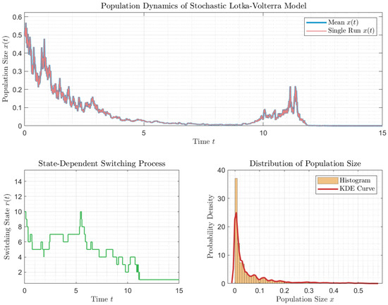
By Theorem 3, the population goes extinct. This is precisely depicted in Figure 1. Here, we take the state space as $\mathcal{S}=\{1,2,\dots ,25\}$.

(2) For any $k\in \mathcal{S}$,

$$b\left(k\right)={\displaystyle \frac{4}{k}}+1,a\left(k\right)=-{\displaystyle \frac{1}{k}},\sigma \left(k\right)\equiv \sqrt{2},D(k,z)=1\wedge {\left|z\right|}^2.$$

Then, we get

$$\begin{array}{cc}\hfill \varphi \left(k\right)=& b\left(k\right)-{\displaystyle \frac{1}{2}}{\sigma }^2\left(k\right)-{\displaystyle \frac{1}{2}}{\int }_{{\mathbb{R}}_0}{D}^2(k,z)\nu \left(\mathrm{d}z\right)\hfill \\ \hfill =& {\displaystyle \frac{4}{k}}-{\int }_0^1{\left|z\right|}^{{\displaystyle \frac{8}{3}}}\mathrm{d}z-{\int }_1^{\infty }{\left|z\right|}^{-{\displaystyle \frac{4}{3}}}dz={\displaystyle \frac{4}{k}}-{\displaystyle \frac{36}{11}},\hfill \\ \hfill \psi \left(k\right)=& {\displaystyle \frac{1}{2}}{\sigma }^2\left(k\right)+{\displaystyle \frac{1}{2}}{\int }_{{\mathbb{R}}_0}{D}^2(k,z)\nu \left(\mathrm{d}z\right)={\displaystyle \frac{47}{11}}.\hfill \end{array}$$

Consider a finite partition: $F=\{F_1,F_2\}$, where $F_1=\left\{1\right\}$, $F_2=\{2,3,\dots \}$. Then,

$$\begin{array}{c}\hfill {\overline{Q}}^F=\left(\begin{array}{cc}-1& 1\\ 3& -3\end{array}\right).\end{array}$$

Moreover,

$${\varphi }_1^F=\varphi \left(1\right)={\displaystyle \frac{8}{11}},{\varphi }_2^F=\underset{j\in F_2}{inf}\varphi \left(j\right)=-{\displaystyle \frac{36}{11}},{\psi }_1^F={\psi }_2^F={\displaystyle \frac{47}{11}}.$$

Thus, we have

$${\gamma }_1\left(\theta \right)={\displaystyle \frac{8}{11}}\theta -{\displaystyle \frac{47}{11}}{\theta }^2,{\gamma }_2\left(\theta \right)=-{\displaystyle \frac{36}{11}}\theta -{\displaystyle \frac{47}{11}}{\theta }^2.$$

Take $C=1$. It is easy to verify that (A1)–(A6) are satisfied. When $0<\theta <{\displaystyle \frac{8}{47}}$, the matrix

$$\begin{array}{c}\hfill \left(\theta diag({\gamma }_1\left(\theta \right),{\gamma }_2\left(\theta \right))-\overline{Q^F}\right){\overline{H}}_2=\left(\begin{array}{cc}{\displaystyle \frac{8}{11}}\theta -{\displaystyle \frac{47}{11}}{\theta }^2& -1\\ -{\displaystyle \frac{36}{11}}\theta -{\displaystyle \frac{47}{11}}{\theta }^2& -{\displaystyle \frac{36}{11}}\theta -{\displaystyle \frac{47}{11}}{\theta }^2+3\end{array}\right)\end{array}$$

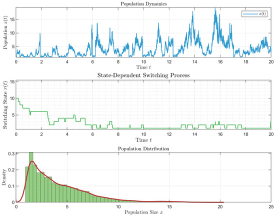
is a nonsingular M-matrix. According to Theorem 4, system (11) is stochastically permanent, which is precisely depicted in Figure 2.

Example 2.

Consider a two-dimensional stochastic Lotka–Volterra model with Lévy jumps and regime-switching in a countable space, satisfying

$$\begin{array}{c}\hfill dx\left(t\right)=\mathrm{diag}(x_1,x_2)\left((b\left(r\left(t\right)\right)+a\left(r\left(t\right)\right)x)dt+\sigma \left(r\left(t\right)\right)\mathrm{d}B\left(t\right)+{\int }_{{\mathbb{R}}_0}D(r\left(t\right),z)\tilde{N}(\mathrm{d}t,\mathrm{d}z)\right).\end{array}$$

(12)

(1). For $k\in \mathcal{S}$, let

$$\begin{array}{c}\hfill b\left(k\right)={\left({\displaystyle \frac{1}{k}},{\displaystyle \frac{1}{k+1}}\right)}^T,a\left(k\right)=\left(\begin{array}{cc}-0.5k& {\displaystyle \frac{1}{3}}\\ {\displaystyle \frac{1}{3}}& -0.5k\end{array}\right),\sigma \left(k\right)=\left(\begin{array}{cc}{\displaystyle \frac{2}{\sqrt{k}}}& 0\\ 0& {\displaystyle \frac{2}{\sqrt{k+1}}}\end{array}\right),D(k,z)=\left(\begin{array}{c}1\wedge {\left|z\right|}^2\\ 1\wedge {\left|z\right|}^2\end{array}\right).\end{array}$$

Recalling

$$\mathsf{\Phi }\left(k\right)=\underset{1⩽i⩽2}{max}\left\{b_i\left(k\right)-{\displaystyle \frac{1}{2}}\sum _{j=1}^2{\sigma }_{ij}^2\left(k\right)+{\int }_{{\mathbb{R}}_0}[log(1+D_i(k,z))-D_i(k,z)]\nu \left(\mathrm{d}z\right)\right\},$$

we obtain

$$\mathsf{\Phi }\left(k\right)=max\left\{-{\displaystyle \frac{1}{k}}-{\displaystyle \frac{36}{5}}-9log2+3\pi ,-{\displaystyle \frac{1}{k+1}}-{\displaystyle \frac{36}{5}}-9log2+3\pi \right\}=-{\displaystyle \frac{1}{k+1}}+2\tilde{M},$$

where $2\tilde{M}=-{\displaystyle \frac{36}{5}}-9log2+3\pi <0$. Let C be the $2\times 2$ identity matrix. Under this setup, assumptions (A1)–(A5) are satisfied, and $\mathsf{\Phi }\left(k\right)=-{\displaystyle \frac{1}{k+1}}+2\tilde{M}$ is an increasing function. The positive series

$$\sum _{k\in \mathcal{S}}{\displaystyle \frac{2}{3^k}}·{\displaystyle \frac{1}{k+1}}+\sum _{k\in \mathcal{S}}{\displaystyle \frac{2}{3^k}}·(-2\tilde{M})$$

is convergent, and

$$\sum _{k\in \mathcal{S}}{\overline{\pi }}_k\mathsf{\Phi }\left(k\right)=\sum _{k\in \mathcal{S}}{\displaystyle \frac{2}{3^k}}\left(-{\displaystyle \frac{1}{k+1}}+2\tilde{M}\right)<0.$$

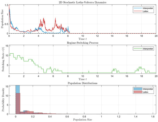
By Theorem 3, the population goes extinct. It can be seen in Figure 3.

(2). For $k\in \mathcal{S}$, let

$$\begin{array}{c}\hfill b\left(k\right)={\left({\displaystyle \frac{4}{k}},{\displaystyle \frac{5}{k}}\right)}^T,a\left(k\right)=\left(\begin{array}{cc}-0.5k& {\displaystyle \frac{1}{3}}\\ {\displaystyle \frac{1}{3}}& -0.5k\end{array}\right),\sigma \left(k\right)=\left(\begin{array}{cc}{\displaystyle \frac{1}{k}}& 0\\ 0& {\displaystyle \frac{1}{k}}\end{array}\right),D(k,z)=\left(\begin{array}{c}1\wedge {\left|z\right|}^2\\ 1\wedge {\left|z\right|}^2\end{array}\right).\end{array}$$

By the definition of ${\varphi }_i\left(k\right)$ and ${\psi }_i\left(k\right)$, we have

$${\varphi }_1\left(k\right)=b_1\left(k\right)-{\displaystyle \frac{1}{2}}{\sigma }_{11}^2\left(k\right)-{\displaystyle \frac{1}{2}}{\int }_{{\mathbb{R}}_0}{D}_1^2(k,z)\nu \left(\mathrm{d}z\right)={\displaystyle \frac{8k-1}{2k^2}}-{\displaystyle \frac{36}{11}},$$

$${\varphi }_2\left(k\right)=b_2\left(k\right)-{\displaystyle \frac{1}{2}}{\sigma }_{22}^2\left(k\right)-{\int }_{{\mathbb{R}}_0}{D}_2^2(k,z)\nu \left(\mathrm{d}z\right)={\displaystyle \frac{10k-1}{2k^2}}-{\displaystyle \frac{36}{11}},$$

$${\psi }_1\left(k\right)={\psi }_2\left(k\right)={\displaystyle \frac{1}{2}}{\sigma }_{11}^2\left(k\right)+{\int }_{{\mathbb{R}}_0}{D}_1^2(k,z)\nu \left(\mathrm{d}z\right)={\displaystyle \frac{1}{2k^2}}+{\displaystyle \frac{36}{11}}.$$

Adopt a finite partition $F=\{F_1,F_2\}$ as $F_1=\left\{1\right\}$, $F_2=\{2,3,\dots \}$. Then, the corresponding parameters are as follows:

$$\begin{array}{c}\hfill \overline{Q^F}=\left(\begin{array}{cc}-1& 1\\ 3& -3\end{array}\right).\end{array}$$

Then,

$${\varphi }_1^F=\underset{j\in F_1}{inf}\min \{{\varphi }_1\left(j\right),{\varphi }_2\left(j\right)\}={\varphi }_1\left(1\right)={\displaystyle \frac{5}{22}},$$

$${\varphi }_2^F=\underset{j\in F_2}{inf}\min \{{\varphi }_1\left(j\right),{\varphi }_2\left(j\right)\}=\underset{j\in F_2}{inf}{\varphi }_1\left(j\right)=-{\displaystyle \frac{36}{11}},$$

$${\psi }_1^F={\psi }_1\left(1\right)={\displaystyle \frac{83}{22}},{\psi }_2^F=\underset{j\in F_2}{sup}{\psi }_1\left(j\right)={\displaystyle \frac{299}{88}}.$$

Thus, we have

$${\gamma }_1\left(\theta \right)={\displaystyle \frac{5}{22}}\theta -{\displaystyle \frac{83}{22}}{\theta }^2,{\gamma }_2\left(\theta \right)=-{\displaystyle \frac{36}{11}}\theta -{\displaystyle \frac{299}{88}}{\theta }^2.$$

Let C be the $2\times 2$ identity matrix. It is easy to verify that (A1)–(A6) are satisfied. Take $0<\theta <{\displaystyle \frac{5}{83}}$; then, the matrix

$$\begin{array}{c}\hfill \left(\theta diag({\gamma }_1\left(\theta \right),{\gamma }_2\left(\theta \right))-{\left(Q^F\right)}^{\ast }\right)H_2^{\ast }=\left(\begin{array}{cc}{\displaystyle \frac{5}{22}}\theta -{\displaystyle \frac{83}{22}}{\theta }^2& -1\\ -{\displaystyle \frac{36}{11}}\theta -{\displaystyle \frac{299}{88}}{\theta }^2& -{\displaystyle \frac{36}{11}}\theta -{\displaystyle \frac{299}{88}}{\theta }^2+3\end{array}\right)\end{array}$$

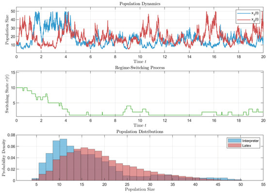
is a nonsingular M-matrix. According to Theorem 4, system (12) is stochastic permanence, which is precisely depicted in Figure 4.

5. Discussion

This paper focused on a multi-group Lotka–Volterra mutualistic model with Lévy jumps and state-dependent switching in a countable state space. We proved that the model admits a unique global positive solution and exhibits properties such as stochastic ultimate boundedness, extinction, and stochastic permanence. These results address our initial hypotheses and extend prior work on stochastic Lotka–Volterra systems.

Our core research aims were to accurately capture mutualistic species dynamics, clarify if species could persist long-term, and find conditions for their permanence or extinction. We showed in our work that countably infinite discrete state models could still be analyzed through a more manageable reduced diffusion system. This has clear biological and ecological value. For complex ecosystems (e.g., multi-species mutualistic networks in fragmented habitats), our framework lets researchers avoid the high computational cost of solving infinite-state models directly. Instead, key questions (e.g., when species persist or go extinct) can be answered by examining the reduced system, greatly lowering computational complexity.

References

- Lotka, A. Elements of Physical Biology; Williams and Wilkins: Philadelphia, PA, USA, 1925. [Google Scholar]
- Volterra, V. Fluctuations in the abundance of a species considered mathematically. Nature 1926, 118, 558–560. [Google Scholar] [CrossRef]
- Khasminskii, R.; Klebaner, F. Long term behavior of solutions of the Lotka-Volterra system under small random perturbations. Ann. Appl. Probab. 2001, 11, 952–963. [Google Scholar] [CrossRef]
- Khasminskii, R.; Potsepun, N. On the replicator dynamics behavior under Stratonovich type random perturbations. Stochastics Dyn. 2006, 6, 197–211. [Google Scholar] [CrossRef]
- Mao, X.; Marion, G.; Renshaw, E. Environmental Brownian noise suppresses explosions in population dynamics. Stoch. Process. Their Appl. 2002, 97, 95–110. [Google Scholar] [CrossRef]
- Mao, X.; Marion, G.; Renshaw, E. Asymptotic behavior of the stochastic Lotka-Volterra model. J. Math. Anal. Appl. 2003, 287, 141–156. [Google Scholar] [CrossRef]
- Yin, G.; Zhu, C. Hybrid Switching Diffusions: Properties and Applications; Springer: New York, NY, USA, 2010. [Google Scholar]
- Chen, S.; Guo, Y.; Zhang, C. Stationary distribution of a stochastic epidemic model with distributed delay under regime switching. J. Appl. Math. Comput. 2024, 70, 789–808. [Google Scholar] [CrossRef]
- Shaikhet, L.; Korobeinikov, A. Persistence and Stochastic Extinction in a Lotka–Volterra Predator–Prey Stochastically Perturbed Model. Mathematics 2024, 12, 1588. [Google Scholar] [CrossRef]
- Ma, C.; Zhang, X.; Yuan, R. Dynamic analysis of a stochastic regime-switching Lotka–Volterracompetitive system with distributed delays and Ornstein–Uhlenbeck process. Chaos Solitons Fractals 2025, 190, 115765. [Google Scholar] [CrossRef]
- Don, S.; Burrage, K.; Helmstedt, K.; Burrage, P. Stability Switching in Lotka-Volterra and Ricker-TypePredator-Prey Systems with Arbitrary Step Size. Axioms 2023, 12, 390. [Google Scholar]
- Luo, Q.; Mao, X. Stochastic population dynamics under regime switching. J. Math. Anal. Appl. 2007, 334, 69–84. [Google Scholar] [CrossRef]
- Li, X.; Jiang, D.; Mao, X. Population dynamical behavior of Lotka-Volterra system under regime switching. J. Comput. Appl. Math. 2009, 232, 427–448. [Google Scholar] [CrossRef]
- Wu, R.; Zou, X.; Wang, K.; Liu, M. Stochastic Lotka-Volterra systems under regime switching with jumps. Filomat 2014, 28, 1907–1928. [Google Scholar] [CrossRef]
- Basak, G.; Bisi, A.; Ghosh, M. Stability of degenerate diffusions with state-dependent switching. J. Math. Anal. Appl. 1999, 240, 219–248. [Google Scholar] [CrossRef][Green Version]
- Shao, J. Invariant measures and Euler-Maruyama’s approximations of state-dependent regime-switching diffusions. SIAM J. Control. Optim. 2018, 56, 3215–3238. [Google Scholar] [CrossRef]
- Ji, H.; Xi, F. Stationary distribution of stochastic population dynamics in state-dependent random environments. Syst. Control. Lett. 2020, 144, 104774. [Google Scholar] [CrossRef]
- Cloez, B.; Hairer, M. Exponential ergodicity for Markov processes with random switching. Bernoulli 2015, 21, 505–536. [Google Scholar] [CrossRef]
- Shao, J. Comparison theorem and stability under perturbation of transition rate matrices for regime-switching processes. J. Appl. Probab. 2024, 61, 540–557. [Google Scholar] [CrossRef]
- Xi, F.; Zhu, C. On Feller and strong Feller properties and exponential ergodicity of regime-switching jump diffusion processes with countable regimes. SIAM J. Control. Optim. 2017, 55, 1789–1818. [Google Scholar] [CrossRef]
- Bui, T.; Yin, G. Hybrid competitive Lotka–Volterra ecosystems: Countable switching states and two-time-scale models. Stoch. Anal. Appl. 2019, 37, 219–242. [Google Scholar] [CrossRef]
- Bao, J.; Shao, J. Asymptotic behavior of SIRS models in state-dependent random environments. Nonlinear Anal. Hybrid Syst. 2020, 38, 100914. [Google Scholar] [CrossRef]
- Berman, A.; Plemmons, R. Nonnegative Matrices in the Mathematical Sciences; Society for Industrial and Applied Mathematics: Philadelphia, PA, USA, 1994. [Google Scholar]
Disclaimer/Publisher’s Note: The statements, opinions and data contained in all publications are solely those of the individual author(s) and contributor(s) and not of MDPI and/or the editor(s). MDPI and/or the editor(s) disclaim responsibility for any injury to people or property resulting from any ideas, methods, instructions or products referred to in the content. |
© 2025 by the authors. Licensee MDPI, Basel, Switzerland. This article is an open access article distributed under the terms and conditions of the Creative Commons Attribution (CC BY) license (https://creativecommons.org/licenses/by/4.0/).