Numerical Approximation for a Nonlocal and Nonlinear Reaction–Diffusion Problem with Robin Boundary Conditions

Abstract

In this paper we consider a reaction–diffusion model with nonlocal diffusion and a nonlinear reaction term analogous to a local reaction–diffusion problem with Robin boundary conditions. Firstly, we investigate the existence of solutions in a two-dimensional spatial domain. Then we attach a semi-implicit numerical scheme by using finite differences in order to approximate the solution. We use the iterative Newton method to numerically solve the resulting implicit problem. Based on theoretical results we generate an adaptive mesh in time that ensures the stability of the corresponding numerical scheme. Numerical experiments that illustrate the effectiveness of the theoretical results are provided.

1. Introduction

We consider the following nonlocal and nonlinear reaction–diffusion problem:

$$\left\{\begin{array}{c}{\displaystyle p\frac{\partial }{\partial t}u(t,x)=p_d\underset{\mathrm{\Omega }}{\int }J(x-y)\left[u(t,y)-u(t,x)\right]dy}\hfill \\ {\displaystyle +p_d\underset{\partial \mathrm{\Omega }}{\int }G(x-y_s)\left[g(t,y_s)-p_{t}u(t,x)\right]d{y}_s}\hfill \\ {\displaystyle +p_r\left[u(t,x)-u^3(t,x)\right]+p_{s}f(t,x),(t,x)\in Q}\hfill \\ {\displaystyle u(0,x)=u_0\left(x\right),x\in \mathrm{\Omega },}\hfill \end{array}\right.$$

(1)

where $u(t,x)$ is the unknown function, $t\in [0,T]$, $x\in \mathrm{\Omega }\subset {\mathbb{R}}^2$ with $\mathrm{\Omega }$ a bounded, closed domain of Lebesgue measure $\left|\mathrm{\Omega }\right|$ with a $C^2$ boundary $\partial \mathrm{\Omega }$, $T>0$, $Q=(0,T]\times \mathrm{\Omega }$, and the following hold:

• $p,p_d$, $p_r$, $p_s$, and $p_t$ are positive values, standing for the speed, diffusion, reaction, source, and thermal transfer parameters, respectively;
• $f(t,·)\in C^{\infty }\left(\mathrm{\Omega }\right)$ and $g(t,·)\in C^{\infty }(\partial \mathrm{\Omega })$ are given real functions;
• $d{y}_s$ represents the surface element in the surface integral;
• J and G are symmetric non-negative real functions in $C^{\infty }\left({\mathbb{R}}^2\right)$ compactly supported in the unit ball such that $\underset{{\mathbb{R}}^2}{\int }J\left(z\right)dz=1$ and $\underset{{\mathbb{R}}^2}{\int }G\left(z\right)dz=1$. We set

  $${\displaystyle C_1=\underset{z\in {\mathbb{R}}^2}{max}\left|J\left(z\right)\right|\mathrm{and}{C}_2=\underset{z\in {\mathbb{R}}^2}{max}\left|G\left(z\right)\right|}$$

  (2)
• $u_0\left(x\right)\in C^{\infty }\left(\mathrm{\Omega }\right)$ is the initial condition.

We denote

$$C=2\left|\mathrm{\Omega }\right|{\displaystyle \frac{p_d}{p}}{C}_1+\overline{c}{\displaystyle \frac{p_d{p}_t}{p^2}}{C}_2+{\displaystyle \frac{p_r}{p}},$$

(3)

where $\overline{c}>0$ in (3) comes from the continuous embedding $L^{\infty }\left(\mathrm{\Omega }\right)\subset L^{\infty }(\partial \mathrm{\Omega })$, which implies that the inequality ${\parallel w\parallel }_{L^{\infty }(\partial \mathrm{\Omega })}\le \overline{c}{\parallel w\parallel }_{L^{\infty }\left(\mathrm{\Omega }\right)}$ holds for every $w\in L^{\infty }\left(\mathrm{\Omega }\right)$ (for details, see [1]).

Let $C_3\in (0,\infty )$ be such that

$$\underset{x\in \mathrm{\Omega }}{\sup }\left|f(t,x)\right|\le C_3,\forall t\in (0,T].$$

(4)

The nonlocal and nonlinear reaction–diffusion problem (1) is important when modeling various real-world phenomena: phase transition and phase transformation, particle systems, image processing, etc.

The integro-differential Equation (1), together with the initial condition, can be seen as a nonlocal version of the following local reaction–diffusion equation with Robin boundary conditions (see [1,2,3] and the references therein):

$$\left\{\begin{array}{cc}{\displaystyle p\frac{\partial }{\partial t}u(t,x)-p_d\mathrm{\Delta }u(t,x)=p_r\left[u(t,x)-u^3(t,x)\right]+p_{s}f(t,x)}\hfill & \mathrm{in}Q\hfill \\ p_d{\displaystyle \frac{\partial }{\partial \mathbf{n}}}u(t,x)+p_{t}u(t,x)=g(t,x)\hfill & \mathrm{in}\mathrm{\Sigma }\hfill \\ u(0,x)=u_0\left(x\right)\hfill & \mathrm{on}\mathrm{\Omega },\hfill \end{array}\right.$$

(5)

where $\mathrm{\Sigma }=(0,T]\times \partial \mathrm{\Omega }$ and n = n$\left(x\right)$ is a vector of the outward unit normal to the boundary $\partial \mathrm{\Omega }$. We also assume that the initial condition $u_0\left(x\right)$ verifies the compatibility condition

$${\displaystyle p_d\frac{\partial }{\partial \mathbf{n}}{u}_0\left(x\right)+p_t{u}_0\left(x\right)=g(0,x)\mathrm{on}\partial \mathrm{\Omega }.}$$

Problem (5) is related to the Allen–Cahn equation, which was a well-established model in Materials Science and can be used to model, for example, order–disorder transitions such as ferromagnetism. This model has been applied to many complex moving interface problems. The nonlinear version occurs in the phase–field transition system where the phase function $u(t,x)$ describes the transition between the solid and liquid phases in the solidification process of a material occupying a region $\mathrm{\Omega }$ (e.g., see [4,5,6]). Robin boundary conditions offer greater flexibility than Dirichlet or Neumann conditions in modeling complex physical phenomena involving boundary interactions. They are used in a variety of scientific and engineering fields, including heat transfer (to model thermal convection or radiation from a surface), electromagnetism (to describe the relationship between electric and magnetic fields on a surface), fluid mechanics (to describe the interaction of a fluid with a solid surface), and quantum physics (to model certain phenomena at the boundary of materials). This type of boundary condition can also be interpreted in the context of biological population dynamics as a way to model the migration and interaction of a population with its external environment at the edge of a domain (e.g., an island, a lake, or a specific geographic area). From a formal point of view, the Neumann and Robin conditions differ by the thermal/heat transfer term $p_{t}u(t,x)$. Moreover, this term brings more difficulties in the proofs of the theoretical results and also in the development of the numerical schemes. Last but not least, the thermal/heat term is a source of instability of the numerical solutions.

The Laplace operator $\mathrm{\Delta }u(t,x)$ is approximated by the integral term ${\displaystyle \underset{\mathrm{\Omega }}{\int }J(x-y)\left[u(t,y)-u(t,x)\right]dy}$, while the surface integral term ${\displaystyle p_d\underset{\partial \mathrm{\Omega }}{\int }G(x-y_s)\left[g(t,y_s)-p_{t}u(t,x)\right]d{y}_s}$ is derived from the boundary condition (5). Both positive kernels $J(·)$ and $G(·)$ take into account the distribution of interactions between particles at sites $x,y\in \mathrm{\Omega }$. Details about the terms $J(x-y)$, ${\displaystyle \underset{\mathrm{\Omega }}{\int }J(x-y)u(t,y)dy}$, and ${\displaystyle -\underset{\mathrm{\Omega }}{\int }J(x-y)u(t,x)dy}$ from (1) can be found in [2,7] and references therein. The integral term $\underset{\partial \mathrm{\Omega }}{\int }G(x-y_s)\left[g(t,y_s)-p_{t}u(t,x)\right]d{y}_s$ takes into account the prescribed flux of individuals that enter or leave the domain according to the sign of g (see [3]).

For theoretical results regarding the well-posedness, existence, and uniqueness of the solutions to the nonlocal problem (1), considering different boundary conditions, we refer to [1,3,7,8,9,10,11,12,13]. Numerical approximations of the corresponding solutions can be found in [1,2,7,8,9,10,11,12,14,15,16].

This paper introduces an adaptive time-step size method to approximate the solution of the nonlocal model (1). This concept of adaptivity means updating the time-step size for each time iteration according to the current state of the system and not using a classical, equidistant mesh in time. For example, this approach is important due to the different time scales that arise in the evolution of phase field models (see [5,6,12]). The size of the time-step is also adjusted taking into account the model parameters and initial data for each time iteration. In the literature, there are various numerical methods with adaptive time-steps that are based on different theoretical results; e.g., in [12], the authors used the local error method to create a non-uniform mesh. Here, we shall use an adaptive time-step method based on Banach fixed point theory, firstly developed in [10] and then improved in [1,8,11,16]. The second section contains some results related to the existence and the uniqueness of the solution to the nonlocal problem (1). Then, using the obtained theoretical results, we introduce a numerical scheme with adaptive time-step size and we perform some numerical experiments that illustrate its effectiveness. These are followed by some conclusions and some possible further work.

2. Existence and Uniqueness of the Solution to Problem (1)

We denote ${\displaystyle X=L^{\infty }((0,T],C^{\infty }(\partial \mathrm{\Omega }))}$. Let us note that we can find a small enough $\overline{t}>0$, depending on $\parallel u_0{\parallel }_{L^{\infty }\left(\mathrm{\Omega }\right)}$ and ${\parallel g\parallel }_X$, that satisfies the following conditions:

$$\left\{\begin{array}{c}{\displaystyle \overline{t}<\frac{1}{C}}\hfill \\ {\displaystyle \frac{p_d}{p}{C}_2\overline{t}{\parallel g\parallel }_X+\frac{p_s}{p}{C}_3\overline{t}+{\parallel u_0\parallel }_{L^{\infty }\left(\mathrm{\Omega }\right)}<\frac{2}{3}\sqrt{\frac{{(1-C\overline{t})}^3}{3\frac{p_r}{p}\overline{t}}},}\hfill \end{array}\right.$$

(6)

where C is given by (3) (for details, see [1,10,11]).

The solutions to the problem (1) belong to the space ${\displaystyle Y=C([0,\overline{t}],C^{\infty }\left(\mathrm{\Omega }\right))}$, with the corresponding norm

$${\displaystyle \left|\parallel u\parallel \right|=\underset{t\in [0,\overline{t}]}{max}{\parallel u(t,·)\parallel }_{L^{\infty }\left(\mathrm{\Omega }\right)}=\underset{t\in [0,\overline{t}]}{max}\underset{x\in \mathrm{\Omega }}{\mathrm{ess}\sup }|u(t,x)|,\forall u\in Y,}$$

as $C^{\infty }\left(\mathrm{\Omega }\right)\subset L^{\infty }\left(\mathrm{\Omega }\right)$.

Following the same steps as in [1], we obtain the unique solution of problem (1) on $[0,\overline{t}]$. Namely, by integrating (1) on $[0,t]$, with $0<t\le \overline{t}$, and using the initial condition (1), we have

$$\begin{array}{cc}u(t,x)=\hfill & {\displaystyle u_0\left(x\right)+\frac{p_d}{p}\underset{0}{\overset{t}{\int }}\underset{\mathrm{\Omega }}{\int }J(x-y)u(s,y)dyds}\hfill \\ \hfill & {\displaystyle -\frac{p_d}{p}\underset{0}{\overset{t}{\int }}\underset{\mathrm{\Omega }}{\int }J(x-y)u(s,x)dyds}\hfill \\ \hfill & {\displaystyle +\frac{p_d}{p}\underset{0}{\overset{t}{\int }}\left\{\underset{\partial \mathrm{\Omega }}{\int }G(x-y)\left[g(s,y)-\frac{p_t}{p}u(s,x)\right]d{y}_s\right\}ds}\hfill \\ \hfill & {\displaystyle +\frac{p_r}{p}\underset{0}{\overset{t}{\int }}\left[u(s,x)-u^3(s,x)\right]ds+\frac{p_s}{p}\underset{0}{\overset{t}{\int }}f(s,x)ds.}\hfill \end{array}$$

(7)

For any $u(t,x)\in Y,$ we define the following operator:

$$\begin{array}{cc}\left(Hu\right)(t,x)=\hfill & {\displaystyle u_0\left(x\right)+\frac{p_d}{p}\underset{0}{\overset{t}{\int }}\underset{\mathrm{\Omega }}{\int }J(x-y)u(s,y)dyds}\hfill \\ \hfill & {\displaystyle -\frac{p_d}{p}\underset{0}{\overset{t}{\int }}\underset{\mathrm{\Omega }}{\int }J(x-y)u(s,x)dyds}\hfill \\ \hfill & {\displaystyle +\frac{p_d}{p}\underset{0}{\overset{t}{\int }}\left\{\underset{\partial \mathrm{\Omega }}{\int }G(x-y)\left[g(s,y)-\frac{p_t}{p}u(s,x)\right]d{y}_s\right\}ds}\hfill \\ \hfill & {\displaystyle +\frac{p_r}{p}\underset{0}{\overset{t}{\int }}\left[u(s,x)-u^3(s,x)\right]ds+\frac{p_s}{p}\underset{0}{\overset{t}{\int }}f(s,x)ds}\hfill \end{array}$$

(8)

with

$$\left(Hu\right)(0,x)=u_0\left(x\right)\in C^{\infty }\left(\mathrm{\Omega }\right),x\in \mathrm{\Omega }.$$

(9)

We will check that

$$\left(Hu\right)(t,·)\in C^{\infty }\left(\mathrm{\Omega }\right),\forall t\in [0,\overline{t}],u\in Y.$$

Let us verify that $\left(Hu\right)(t,x)\in Y,(t,x)\in Q$, $\forall u(t,x)\in Y$. In order to draw this conclusion, we take the first integral term:

$${\displaystyle I_1(t,x)=\frac{p_d}{p}\underset{0}{\overset{t}{\int }}\underset{\mathrm{\Omega }}{\int }J(x-y)u(s,y)dyds}$$

which satisfies the inequality

$${\displaystyle |I_1(t,x)|\le \frac{p_d}{p}{C}_1{C}_4\left|\mathrm{\Omega }\right|\overline{t},\forall t\in [0,\overline{t}],\mathrm{a}.\mathrm{p}.\mathrm{t}.x\in \mathrm{\Omega },}$$

where $C_4\in (0,+\infty )$ is given by the following inequality:

$${\parallel u(t,·)\parallel }_{L^{\infty }\left(\mathrm{\Omega }\right)}\le C_4,\forall t\in [0,\overline{t}],$$

resulting from the fact that $u(t,·)\in C^{\infty }\left(\mathrm{\Omega }\right)\subset L^{\infty }\left(\mathrm{\Omega }\right).$ Indeed,

$$\begin{array}{c}|I_1(t,x)|=\left|\frac{p_d}{p}\underset{0}{\overset{t}{\int }}\underset{\mathrm{\Omega }}{\int }J(x-y)u(s,y)dyds\right|\hfill \\ {\displaystyle \le \frac{p_d}{p}\underset{0}{\overset{t}{\int }}\left|\underset{\mathrm{\Omega }}{\int }J(x-y)u(s,y)dy\right|ds\le \frac{p_d}{p}\underset{0}{\overset{t}{\int }}\underset{\mathrm{\Omega }}{\int }\left|J(x-y)\right|\left|u(s,y)\right|dyds}\hfill \\ {\displaystyle \le \frac{p_d}{p}{C}_1\underset{0}{\overset{t}{\int }}\underset{\mathrm{\Omega }}{\int }\left|u(s,y)\right|dyds\le \frac{p_d}{p}{C}_1\underset{0}{\overset{t}{\int }}\underset{\mathrm{\Omega }}{\int }\underset{y\in \mathrm{\Omega }}{\mathrm{ess}\sup }|u(t,y)|dyds}\hfill \\ {\displaystyle =\frac{p_d}{p}{C}_1\underset{0}{\overset{t}{\int }}\left[\underset{y\in \mathrm{\Omega }}{\mathrm{ess}\sup }|u(t,y)|\underset{\mathrm{\Omega }}{\int }dy\right]ds=\frac{p_d}{p}{C}_1\underset{0}{\overset{t}{\int }}\left[\underset{y\in \mathrm{\Omega }}{\mathrm{ess}\sup }|u(t,y)||\mathrm{\Omega }|\right]ds}\hfill \\ {\displaystyle =\frac{p_d}{p}{C}_1|\mathrm{\Omega }|\underset{0}{\overset{t}{\int }}{\parallel u(t,·)\parallel }_{L^{\infty }\left(\mathrm{\Omega }\right)}ds\le \frac{p_d}{p}{C}_1{C}_4|\mathrm{\Omega }|\underset{0}{\overset{t}{\int }}ds\le \frac{p_d}{p}{C}_1{C}_4|\mathrm{\Omega }|\overline{t}.}\hfill \end{array}$$

Consequently,

$${\displaystyle \underset{x\in \mathrm{\Omega }}{\mathrm{ess}\sup }\left|I_1(t,x)\right|<\infty ,\forall t\in [0,\overline{t}],\mathrm{a}.\mathrm{p}.\mathrm{t}.x\in \mathrm{\Omega },}$$

i.e., $I_1(t,·)\in L^{\infty }\left(\mathrm{\Omega }\right),\forall t\in [0,\overline{t}]$. In a similar way we prove that the other integral terms of (8) also belong to $L^{\infty }\left(\mathrm{\Omega }\right),\forall t\in [0,\overline{t}]$.

Lemma 1.

If $u_0\left(x\right)\in C^{\infty }\left(\mathrm{\Omega }\right)$, $f(t,·)\in C^{\infty }\left(\mathrm{\Omega }\right)$, and $g(t,·)\in C^{\infty }(\partial \mathrm{\Omega })$, then the operator H, given by (8) and (9), is well defined.

Proof. 

We take $u(·,·)\in Y$ and $t_1,t_2\in [0,\overline{t}]$, with $t_1<t_2$, and we obtain

$$\begin{array}{cc}\hfill & {\displaystyle \parallel \left(Hu\right)(t_1,·)-\left(Hu\right)(t_2,·){\parallel }_{L^{\infty }\left(\mathrm{\Omega }\right)}=\underset{x\in \mathrm{\Omega }}{\mathrm{ess}\sup }|\left(Hu\right)(t_1,x)-\left(Hu\right)(t_2,x)|}\hfill \\ \hfill & {\displaystyle =\underset{x\in \mathrm{\Omega }}{\mathrm{ess}\sup }|\frac{p_d}{p}\underset{t_1}{\overset{t_2}{\int }}\underset{\mathrm{\Omega }}{\int }J(x-y)\left[u(s,y)-u(s,x)\right]dyds}\hfill \\ \hfill & {\displaystyle +\frac{p_d}{p}\underset{t_1}{\overset{t_2}{\int }}\left\{\underset{\partial \mathrm{\Omega }}{\int }G(x-y)[g(s,y)-\frac{p_t}{p}u(s,x)]d{y}_s\right\}ds}\hfill \\ \hfill & {\displaystyle +\frac{p_r}{p}\underset{t_1}{\overset{t_2}{\int }}\left[u(s,x)-u^3(s,x)\right]ds+\frac{p_s}{p}\underset{t_1}{\overset{t_2}{\int }}f(s,x)ds|.}\hfill \end{array}$$

Then we have the inequality

$${\displaystyle \parallel \left(Hu\right)(t_1,·)-\left(Hu\right)(t_2,·){\parallel }_{L^{\infty }\left(\mathrm{\Omega }\right)}\le C_5(t_2-t_1),}$$

(10)

where

$$C_5=2\left|\mathrm{\Omega }\right|{\displaystyle \frac{p_d}{p}}{C}_1\left|\parallel u\parallel \right|+{\displaystyle \frac{p_d}{p}}{C}_2{\parallel g\parallel }_X+\overline{c}{\displaystyle \frac{p_d{p}_t}{p^2}}{C}_2\left|\parallel u\parallel \right|+{\displaystyle \frac{p_r}{p}}\left[\right|\parallel u\parallel |+|\parallel u\parallel {{\displaystyle |}}^3]+{\displaystyle \frac{p_s}{p}}{C}_3.$$

(11)

So, the operator H defined by (8) and (9) is Lipschitz continuous on $(0,\overline{t}]$, with the Lipschitz constant $C_5$ given by (11). Then we have

$$\parallel \left(Hu\right)(t,·)-u_0{\left(x\right)\parallel }_{L^{\infty }\left(\mathrm{\Omega }\right)}\le C_{5}t,\forall t\in [0,\overline{t}].$$

(12)

From (10) and (12) we obtain that the operator H is continuous on $[0,\overline{t}]$, so $H:Y\to Y$ is well defined.    □

Remark 1.

If we take $u\in B(0,r)$, where $B(0,r)$ stands for the closed ball of Y, meaning that $|\parallel u\parallel |\le r$, we get the inequality (10) with

$$C_5\le \left(2\left|\mathrm{\Omega }\right|{\displaystyle \frac{p_d}{p}}{C}_1+\overline{c}{\displaystyle \frac{p_d{p}_t}{p^2}}{C}_2+{\displaystyle \frac{p_r}{p}}\right)r+{\displaystyle \frac{p_d}{p}}{C}_2{\parallel g\parallel }_X+{\displaystyle \frac{p_r}{p}}{r}^3+{\displaystyle \frac{p_s}{p}}{C}_3$$

or (see (3))

$$C_5\le Cr+{\displaystyle \frac{p_d}{p}}{C}_2{\parallel g\parallel }_X+{\displaystyle \frac{p_r}{p}}{r}^3+{\displaystyle \frac{p_s}{p}}{C}_3=C_6.$$

By imposing that $C_6<1,$ we have that H is a contraction.

The space ${\displaystyle Y=C([0,\overline{t}],C^{\infty }\left(\mathrm{\Omega }\right))}$ is complete, as a subspace of ${\displaystyle C([0,\overline{t}],L^{\infty }\left(\mathrm{\Omega }\right))}$, which is complete. Consequently, we have that the operator H admits a unique fixed point, so problem (1) has a unique solution.

Our further goal is to find $r>0$ such that $H\left(B(0,r)\right)\subset B(0,r)$; therefore the solution is stable. To do so, we prove the two theorems below.

Theorem 1.

There exists $r=r\left(\overline{t}\right)>0$ such that

$$\parallel u_0{\parallel }_{L^{\infty }\left(\mathrm{\Omega }\right)}+\left({\displaystyle \frac{p_r}{p}}{r}^3+Cr+{\displaystyle \frac{p_d}{p}}{C}_2{\parallel g\parallel }_X+{\displaystyle \frac{p_s}{p}}{C}_3\right)\overline{t}\le r$$

and

$$\left(3{\displaystyle \frac{p_r}{p}}{r}^2+C\right)\overline{t}<1,$$

where $\overline{t}>0$ satisfies (6).

Proof. 

We consider the function

$$h\left(x\right)={\displaystyle \frac{p_r}{p}}\overline{t}{x}^3+(C\overline{t}-1)x+\left({\displaystyle \frac{p_d}{p}}{C}_2{\parallel g\parallel }_X+{\displaystyle \frac{p_s}{p}}{C}_3\right)\overline{t}+{\parallel u_0\parallel }_{L^{\infty }\left(\mathrm{\Omega }\right)},$$

with

$$h^{\prime }\left(x\right)=3{\displaystyle \frac{p_r}{p}}\overline{t}{x}^2+C\overline{t}-1.$$

We have that ${\displaystyle \frac{p_r}{p}\overline{t}>0}$, ${\displaystyle (C\overline{t}-1)<0}$ (see (6)) and ${\displaystyle \left(\frac{p_d}{p}{C}_2{\parallel g\parallel }_X+\frac{p_s}{p}{C}_3\right)\overline{t}+{\parallel u_0\parallel }_{L^{\infty }\left(\mathrm{\Omega }\right)}>0}$, and from (6) we also have

$${\displaystyle \frac{2}{3}(C\overline{t}-1)\sqrt{-\frac{(C\overline{t}-1)}{3\frac{p_r}{p}\overline{t}}}+\left(\frac{p_d}{p}{C}_2{\parallel g\parallel }_X+\frac{p_s}{p}{C}_3\right)\overline{t}+{\parallel u_0\parallel }_{L^{\infty }\left(\mathrm{\Omega }\right)}<0.}$$

Now, we may apply Proposition 2.1 from [1], where ${\displaystyle a=\frac{p_r}{p}\overline{t}>0}$, ${\displaystyle b=(C\overline{t}-1)<0}$ and ${\displaystyle c=\left(\frac{p_d}{p}{C}_2{\parallel g\parallel }_X+\frac{p_s}{p}{C}_3\right)\overline{t}+{\parallel u_0\parallel }_{L^{\infty }\left(\mathrm{\Omega }\right)}>0.}$ If

$${\displaystyle \frac{2}{3}}b\sqrt{-{\displaystyle \frac{b}{3a}}}+c<0,$$

then there exists $z\in (0,\infty )$ such that

$$h\left(z\right)<0.$$

We note that the hypothesis of the proposition is satisfied, and the technique that gives the z point such that the function in z is negative is described in the following. Due to the monotonicity of h, it results that ${\displaystyle x_1=\sqrt{\frac{1-C\overline{t}}{3\frac{p_r}{p}\overline{t}}}}$ is the positive root of $h^{\prime }$ and so

$${\displaystyle \underset{x\in (0,\infty )}{min}h\left(x\right)=h\left(x_1\right)=h\left(\sqrt{\frac{1-C\overline{t}}{3\frac{p_r}{p}\overline{t}}}\right)<0.}$$

Due to the continuity of h and because $h\left(x_1\right)<0<h\left(0\right)$, there exist a unique $z_1\in (0,x_1)$ such that $h\left(z_1\right)=0$ and $h\left(z\right)<0,\forall z\in (z_1,x_1)$ and a unique $z_2\in (x_1,+\infty )$ such that $h\left(z_2\right)=0$ and $h\left(z\right)<0,\forall z\in (x_1,z_2)$. So, we may find ${\displaystyle r\in \left[z_1,z_2\right]}$ such that $h\left(r\right)<0$ and $h^{\prime }\left(r\right)<0$, which are equivalent to the conclusions of the theorem.    □

Theorem 2.

The operator H defined in (8) and (9) maps $B(0,r)$ into itself, where $\overline{t}$ and r are given by Theorem 1.

Proof. 

For any $u\in Y$ and $t_1,t_2\in [0,\overline{t}]$, $t_1<t_2$, we know (see Lemma 1)

$$\begin{array}{ccc}& & \parallel (Hu(t_1,·)-\left(Hu\right)(t_2,·){\parallel }_{L^{\infty }\left(\mathrm{\Omega }\right)}\le [{\displaystyle \frac{p_r}{p}}|\parallel u\parallel {|}^3\hfill \\ & & +\left(2\left|\mathrm{\Omega }\right|{\displaystyle \frac{p_d}{p}}{C}_1+\overline{c}{\displaystyle \frac{p_d{p}_t}{p^2}}{C}_2+{\displaystyle \frac{p_r}{p}}\right)\left|\parallel u\parallel \right|+{\displaystyle \frac{p_d}{p}}{C}_2{\parallel g\parallel }_X+{\displaystyle \frac{p_s}{p}}{C}_3](t_2-t_1).\hfill \end{array}$$

We take $u\in B(0,r)$, meaning that ${\displaystyle |}\parallel u\parallel {\displaystyle |}\le r$, and we get that

$$\begin{array}{ccc}& & {\parallel \left(Hu\right)(t,·)-\left(Hu\right)(0,·)\parallel }_{L^{\infty }\left(\mathrm{\Omega }\right)}\hfill \\ \hfill & & \le \left[{\displaystyle \frac{p_r}{p}}{r}^3+\left(2\left|\mathrm{\Omega }\right|{\displaystyle \frac{p_d}{p}}{C}_1+\overline{c}{\displaystyle \frac{p_d{p}_t}{p^2}}{C}_2+{\displaystyle \frac{p_r}{p}}\right)r+{\displaystyle \frac{p_d}{p}}{C}_2{\parallel g\parallel }_X+{\displaystyle \frac{p_s}{p}}{C}_3+{\displaystyle \frac{p_d}{p}}\right]t,\hfill \end{array}$$

$\forall t,0\le t\le \overline{t}$. Using (3) and Theorem 1, it follows that

$$\begin{array}{ccc}& & {\parallel Hu(t,·)\parallel }_{L^{\infty }\left(\mathrm{\Omega }\right)}\le {\parallel u_0\parallel }_{L^{\infty }\left(\mathrm{\Omega }\right)}+\left({\displaystyle \frac{p_r}{p}}{r}^3+Cr+{\displaystyle \frac{p_d}{p}}{C}_2{\parallel g\parallel }_X+{\displaystyle \frac{p_s}{p}}{C}_3\right)\overline{t}\le r.\hfill \end{array}$$

It follows that

$$\left|\parallel Hu\parallel \right|=\underset{t\in [0,\overline{t}]}{max}{\parallel Hu(t,·)\parallel }_{L^{\infty }\left(\mathrm{\Omega }\right)}\le r.$$

  □

We may conclude that the fixed point of the operator H defined by (8) and (9) is the unique solution of the problem (1) on $(0,\overline{t}]$.

Remark 2.

To find a solution on an interval larger than $(0,\overline{t}]$, with $\overline{t}$ satisfying (6), we consider the same problem as (1), but with the initial condition $u_1\left(x\right)=u(\overline{t},x),x\in \mathrm{\Omega }$. We can now find the solution on $[\overline{t},\overline{t}+{\overline{t}}_1]$, where ${\overline{t}}_1$ satisfies

$$\left\{\begin{array}{c}{\displaystyle {\overline{t}}_1<\frac{1}{C}}\hfill \\ {\displaystyle \frac{p_d}{p}{C}_2{\overline{t}}_1{\parallel g\parallel }_X+\frac{p_s}{p}{C}_3{\overline{t}}_1+{\parallel u_1\parallel }_{L^{\infty }\left(\mathrm{\Omega }\right)}<\frac{2}{3}\sqrt{\frac{{(1-C{\overline{t}}_1)}^3}{3\frac{p_r}{p}{\overline{t}}_1}}.}\hfill \end{array}\right.$$

Following the same technique, we can obtain a solution defined on some time interval $[0,T]$, where $T=\overline{t}+{\overline{t}}_1+\dots {\overline{t}}_n$, where by n we denote the number of time iterations required to obtain the solution on $[0,T]$.

3. Numerical Approximation

In order to approximate the solution to the nonlocal and nonlinear reaction–diffusion problem (1), we propose a semi-implicit numerical scheme based on finite differences and the iterative Newton method. To do so, we shall use a forward finite difference formula for the time derivative of u with an order of accuracy of $\mathcal{O}\left(h_t\right)$, where $h_t$ is the difference between two successive time points where the solution is approximated. The numerical method is a semi-implicit and not fully implicit one because not all of the terms can be evaluated at the current moment in time. Thus, for the integral terms in Equation (1), the evaluations from the time point before the current one will be used.

The numerical methods proposed, for example, in [1,8,10,11,16] with the aim of approximating the solutions of various related problems with different boundary conditions are explicit and therefore may encounter stability problems. In addition, the nonlinearity of the reaction term was also treated in the mentioned papers in an explicit manner, considering that the reaction is given only by the solution from the moment of time before the current one. We propose to eliminate these shortcomings using a semi-implicit method, approaching the resulting nonlinear system with the Newton iterative method.

We consider the rectangular domain $\mathrm{\Omega }=[a,b]\times [c,d]\subset {\mathbb{R}}^2$. To approximate the problem in $\mathrm{\Omega }$ (a two-dimensional space), we introduce a computational grid by considering equidistant discretization nodes for both axes corresponding to $\mathrm{\Omega }$, $Ox$ and $Oy$. To do so, we discretize $[a,b]$ by the finite set

$$M_x=\left\{x_0,x_1,\dots ,x_{N_x+1}\right\},$$

where

$$x_j=x_0+j{h}_x,j=0,1,\dots ,N_x+1,\mathrm{with}{h}_x={\displaystyle \frac{b-a}{N_x+1}},x_0=a,x_{N_x+1}=b,$$

and the interval $[c,d]$ by the finite set

$$M_y=\left\{y_0,y_1,\dots ,y_{N_y+1}\right\},$$

where

$$y_k=y_0+k{h}_y,k=0,1,\dots ,N_y+1,\mathrm{with}{h}_y={\displaystyle \frac{d-c}{N_y+1}},y_0=c,y_{N_y+1}=d.$$

With these notations, the Cartesian product

$$\begin{array}{cc}\hfill {\mathrm{\Omega }}_{x,y}& =M_x\times M_y\hfill \\ & =\{(x_j,y_k),x_j\in M_x,y_k\in M_y,j=0,1,\dots ,N_x+1,k=0,1,\dots ,N_y+1\}\hfill \end{array}$$

represents the computational grid on $\mathrm{\Omega }$. By $\partial {\mathrm{\Omega }}_{x,y}$ we will denote the subset of grid points from ${\mathrm{\Omega }}_{x,y}$ which are on the boundary $\partial \mathrm{\Omega }$.

We consider $[0,\overline{t}]$, with $0=t_0<t_1\le \overline{t}$, where $\overline{t}$ satisfies the inequalities (6), and denote by $u_{j,k}^1$ the approximation of the unique solution $u(t,x)$ of (1) at each grid point $(t_1,x_j,y_k)$, where $(x_j,y_k)\in {\mathrm{\Omega }}_{x,y}$, $j=0,1,\dots ,N_x+1$, and $k=0,1,\dots ,N_y+1$. Corresponding to the initial condition (1), we have $u_{j,k}^0=u_0(x_j,y_k)$ at each grid point $(t_0,x_j,y_k)$, where $(x_j,y_k)\in {\mathrm{\Omega }}_{x,y}$ for $j=0,1,\dots ,N_x+1$, and $k=0,1,\dots ,N_y+1$.

In the following, we shall use a semi-implicit numerical scheme based on finite difference approximations of Equation (1). The approximation system corresponding to (1) on $[0,\overline{t}]$ is

$$\left\{\begin{array}{cc}{\displaystyle p\frac{u_{j,k}^1-u_{j,k}^0}{t_1}=p_d{J}_{j,k}^0+p_d{G}_{j,k}^0+p_r\left[u_{j,k}^1-{\left(u_{j,k}^1\right)}^3\right]+p_s{f}_{j,k}^1}\hfill & \mathrm{in}{\mathrm{\Omega }}_{x,y},\hfill \\ u_{j,k}^0=u_0(x_j,y_k)\hfill & \mathrm{on}{\mathrm{\Omega }}_{x,y},\hfill \end{array}\right.$$

(13)

where

$$\begin{array}{c}{\displaystyle f_{j,k}^1=f(t_1,x_j,y_k),}\hfill \\ {\displaystyle J_{j,k}^0=\underset{\mathrm{\Omega }}{\int }J(x_{j,k}-y)\left[u^0\left(y\right)-u_{j,k}^0\right]dy,}\hfill \\ {\displaystyle G_{j,k}^0=\underset{\partial \mathrm{\Omega }}{\int }G(x_{j,k}-y_s)\left[g(t_0,y_s)-p_t{u}_{j,k}^0\right]d{y}_s,}\hfill \end{array}$$

(14)

for $j=0,1,\dots ,N_x+1$ and $k=0,1,\dots ,N_y+1.$

We use the iterated trapezoidal rule to approximate the integral terms of $J_{j,k}^0$ such that we have

$$\begin{array}{c}{\displaystyle J_{j,k}^0=h_x{h}_y\{\sum _{d=1}^{N_x}\sum _{l=1}^{N_y}J(x_{j,k}-y_{d,l})\left(u_{d,l}^0-u_{j,k}^0\right)}\hfill \\ {\displaystyle +\frac{1}{2}\sum _{d=1}^{N_x}\left[J(x_{j,k}-y_{d,0})\left(u_{d,0}^0-u_{j,k}^0\right)+J(x_{j,k}-y_{d,N_y+1})\left(u_{d,N_y+1}^0-u_{j,k}^0\right)\right]}\hfill \\ {\displaystyle +\frac{1}{2}\sum _{l=1}^{N_y}\left[J(x_{j,k}-y_{0,l})\left(u_{0,l}^0-u_{j,k}^0\right)+J(x_{j,k}-y_{N_x+1,l})\left(u_{N_x+1,l}^0-u_{j,k}^0\right)\right]}\hfill \\ {\displaystyle +\frac{1}{4}[J(x_{j,k}-y_{0,0})\left(u_{0,0}^0-u_{j,k}^0\right)+J(x_{j,k}-y_{N_x+1,0})\left(u_{N_x+1,0}^0-u_{j,k}^0\right)}\hfill \\ {\displaystyle +J(x_{j,k}-y_{0,N_y+1})\left(u_{0,N_y+1}^0-u_{j,k}^0\right)}\hfill \\ {\displaystyle +J(x_{j,k}-y_{N_x+1,N_y+1})\left(u_{N_x+1,N_y+1}^0-u_{j,k}^0\right)]{\displaystyle \}},}\hfill \end{array}$$

(15)

and

$$\begin{array}{c}{\displaystyle G_{j,k}^0=h_x\left\{\sum _{d=1}^{N_x}\right[G(x_{j,k}-y_{d,0})\left(g_{d,0}^0-p_t{u}_{j,k}^0\right)}\hfill \\ {\displaystyle +G(x_{j,k}-y_{d,N_y+1})\left(g_{d,N_y+1}^0-p_t{u}_{j,k}^0\right)]}\hfill \\ {\displaystyle +\frac{1}{2}[G(x_{j,k}-y_{0,0})\left(g_{0,0}^0-p_t{u}_{j,k}^0\right)+G(x_{j,k}-y_{N_x+1,0})\left(g_{N_x+1,0}^0-p_t{u}_{j,k}^0\right)}\hfill \\ {\displaystyle +G(x_{j,k}-y_{0,N_y+1})\left(g_{0,N_y+1}^0-p_t{u}_{j,k}^0\right)}\hfill \\ {\displaystyle +G(x_{j,k}-y_{N_x+1,N_y+1})\left(g_{N_x+1,N_y+1}^0-p_t{u}_{j,k}^0\right)]{\displaystyle \}}}\hfill \\ {\displaystyle +h_y\left\{\sum _{l=1}^{N_y}\right[G(x_{j,k}-y_{0,l})\left(g_{0,l}^0-p_t{u}_{j,k}^0\right)}\hfill \\ {\displaystyle +G(x_{j,k}-y_{N_x+1,l})\left(g_{N_x+1,l}^0-p_t{u}_{j,k}^0\right)}\hfill \\ {\displaystyle +\frac{1}{2}[G(x_{j,k}-y_{0,0})\left(g_{0,0}^0-p_t{u}_{j,k}^0\right)+G(x_{j,k}-y_{N_x+1,0})\left(g_{N_x+1,0}^0-p_t{u}_{j,k}^0\right)}\hfill \\ {\displaystyle +G(x_{j,k}-y_{0,N_y+1})\left(g_{0,N_y+1}^0-p_t{u}_{j,k}^0\right)}\hfill \\ {\displaystyle +G(x_{j,k}-y_{N_x+1,N_y+1})\left(g_{N_x+1,N_y+1}^0-p_t{u}_{j,k}^0\right)]{\displaystyle \}},}\hfill \end{array}$$

(16)

where

${\displaystyle g_{d,0}^0=g(0,y_{d,0})}$, $y_{d,0}\in \partial {\mathrm{\Omega }}_{x,y}$,   

${\displaystyle g_{d,N_y+1}^0=g(0,y_{d,N_y+1})}$, $y_{d,N_y+1}\in \partial {\mathrm{\Omega }}_{x,y}$, $d=0,1,\dots ,N_x+1$;   

${\displaystyle g_{0,l}^0=g(0,y_{0,l})}$, $y_{0,l}\in \partial {\mathrm{\Omega }}_{x,y}$,   

${\displaystyle g_{N_x+1,l}^0=g(0,y_{N_x+1,l})}$, $y_{N_x+1,l}\in \partial {\mathrm{\Omega }}_{x,y}$, $l=0,1,\dots ,N_y+1$.

Thus, from (13) we get the following numerical approximation scheme to problem (1) on $[0,\overline{t}]$:

$${\displaystyle (p-p_r{t}_1)u_{j,k}^1+p_r{t}_1{\left(u_{j,k}^1\right)}^3=p{u}_{j,k}^0+p_d{t}_1{J}_{j,k}^0+p_d{t}_1{G}_{j,k}^0+p_s{t}_1{f}_{j,k}^1.}$$

(17)

We consider the column vectors

$$\begin{array}{cc}\hfill U^i=& (u_{0,0}^i,u_{0,1}^i,\dots ,u_{0,N_y+1}^i,u_{1,0}^i,u_{1,1}^i,\dots ,u_{1,N_y+1}^i,\hfill \\ & \dots ,u_{N_x+1,0}^i,u_{N_x+1,1}^i,\dots ,u_{N_x+1,N_y+1}^i{)}^T,\hfill \end{array}$$

(18)

with $dim=(N_x+2)(N_y+2)$ elements and

$$\begin{array}{cc}\hfill W^i=& ({\left(u_{0,0}^i\right)}^3,{\left(u_{0,1}^i\right)}^3,\dots ,{\left(u_{0,N_y+1}^i\right)}^3,\dots ,{\left(u_{N_x+1,0}^i\right)}^3,{\left(u_{N_x+1,1}^i\right)}^3,\hfill \\ & \dots ,{\left(u_{N_x+1,N_y+1}^i\right)}^3{)}_{dim\times 1,}\hfill \end{array}$$

(19)

for each time level $i=0$ or $i=1$. We also make the following notations:

$$a_1=p-p_r{t}_1,a_2=p_r{t}_1,a_3=p_d{t}_1,a_4=p_s{t}_1.$$

We can rewrite the discrete system (17) as follows:

$$a_1{U}^1+a_2{W}^1=p{U}^0+a_3(J^0+G^0)+a_4{f}^1,$$

(20)

where

$$\begin{array}{cc}\hfill J^0=& (J_{0,0}^0,J_{0,1}^0,\dots ,J_{0,N_y+1}^0,J_{1,0}^0,J_{1,1}^0,\dots ,J_{1,N_y+1}^0,\hfill \\ & \dots ,J_{N_x+1,0}^0,J_{N_x+1,1}^0,\dots ,J_{N_x+1,N_y+1}^0{)}_{dim\times 1}\hfill \\ \hfill G^0=& (G_{0,0}^0,G_{0,1}^0,\dots ,G_{0,N_y+1}^0,G_{1,0}^0,G_{1,1}^0,\dots ,G_{1,N_y+1}^0,\hfill \\ & \dots ,G_{N_x+1,0}^0,G_{N_x+1,1}^0,\dots ,G_{N_x+1,N_y+1}^0{)}_{dim\times 1.}\hfill \end{array}$$

In order to approximate the solution for the first time level, we shall use the iterative Newton method. From (20) it follows that we have to solve a nonlinear equation of the form

$$F\left(U^1\right)=0,$$

where

$$F\left(U^1\right)=a_1{U}^1+a_2{W}^1-p{U}^0-a_3(J^0+G^0)-a_4{f}^1.$$

(21)

Let us recall that at each Newton iteration $n=0,1,2,\dots$, we have

$$U^{1,n+1}=U^{1,n}-J_F^{-1}\left(U^{1,n}\right)F\left(U^{1,n}\right),$$

(22)

where

$$\begin{array}{cc}\hfill & U^{1,0}=U^0,J_F\left(U^1\right)=a_1+3a_2{V}^1,\hfill \\ \hfill & V^1=({\left(u_{0,0}^1\right)}^2,{\left(u_{0,1}^1\right)}^2,\dots ,{\left(u_{0,N_y+1}^1\right)}^2,\dots ,{\left(u_{N_x+1,0}^1\right)}^2,{\left(u_{N_x+1,1}^1\right)}^2,\hfill \\ & \dots ,{\left(u_{N_x+1,N_y+1}^1\right)}^2{)}_{dim\times 1}.\hfill \end{array}$$

(23)

By left multiplication of (22) by $J_F\left(U^{1,n}\right)$, we obtain that $U^{1,n+1}$ is the solution of the linear system

$$J_F\left(U^{1,n}\right)U^{1,n+1}=J_F\left(U^{1,n}\right)U^{1,n}-F\left(U^{1,n}\right).$$

(24)

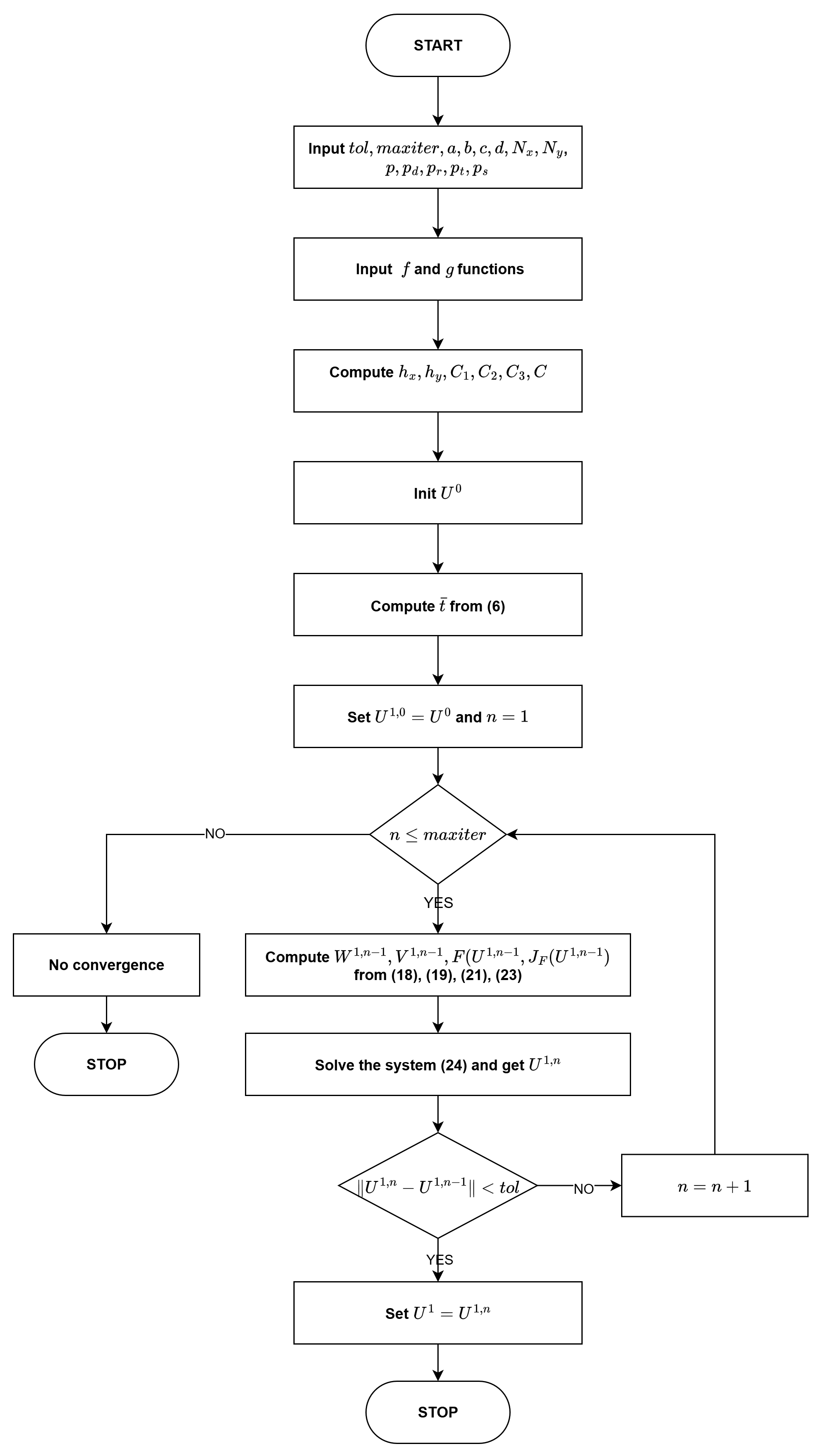
At this point we can develop the numerical approximation algorithm that will solve our problem on $[0,\overline{t}]$. Let us summarize the steps required to start this algorithm:

• We need to obtain the approximation system (17) of the problem (1) that includes the Robin-type conditions in the surface integral term—for this we will use the semi-implicit finite difference scheme described above;
• We need to write (17) in matrix form (20);
• We need to obtain and solve the linear system (24) for each Newton iteration.

The conceptual algorithm can be described in pseudocode as follows (Algorithm 1):

Algorithm 1: NEWTON ALGORITHM

Input:

$tol,maxiter,a,b,c,d$, $N_x$, $N_y$

p, $p_d$, $p_r$, $p_t$, $p_s$, $f,g$

$h_x$, $h_y$, $C_1$, $C_2$, $C_3$, C

Output:

$U^1$—the approximative solution of (1) at $\overline{t}$

Initialize $U^0$

Compute $\overline{t}$ from (6)

$U^{1,0}=U^0$

For $n=1$ to $maxiter$

Compute $W^{1,n-1}$, $V^{1,n-1}$, $F\left(U^{1,n-1}\right)$, $J_F\left(U^{1,n-1}\right)$ from (18), (19), (21), (23)

Solve the system (24) and get the solution $U^{1,n}$

If ${\displaystyle \left|\right|U^{1,n}-U^{1,n-1}\left|\right|<tol}$ then break

If $n<=maxiter$

$U^1=U^{1,n}$

Else

‘No convergence’

The flow chart of the NEWTON ALGORITHM can be viewed in Figure 1.

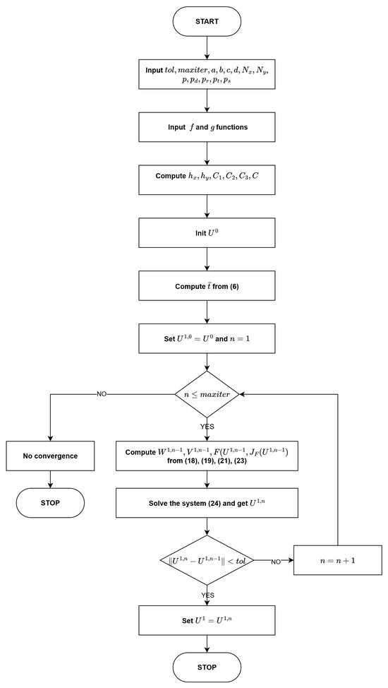
Figure 1. Flow chart of Newton algorithm.

The algorithm continues to iterate until the difference between two consecutive approximations is sufficiently small (tol is a prescribed tolerance) or it stops when it reaches a specific number of iterations (maxiter is the maximum number of Newton iterations).

Using the NEWTON ALGORITHM and continuing the procedure in the manner suggested by Remark 2, we can find the approximate solution to problem (1) on a larger interval of time than $[0,\overline{t}]$.

4. Numerical Experiments

For the computational experiments we set $\mathrm{\Omega }$ to be the rectangle $[-1,1]\times [-1,1]$ ($a=-1,b=1,c=-1,d=1$). We also consider the rescaled kernels

$${\displaystyle J_{\epsilon }\left(z\right)=\frac{1}{{\epsilon }^2}J\left(\frac{z}{\epsilon }\right)\mathrm{and}{G}_{\epsilon }\left(z\right)=\frac{1}{{\epsilon }^2}G\left(\frac{z}{\epsilon }\right),}$$

with

$${\displaystyle J\left(\frac{z}{\epsilon }\right)=G\left(\frac{z}{\epsilon }\right)=\frac{1}{2\pi }{e}^{-\frac{(x^2+y^2)}{2{\epsilon }^2}},z=(x,y)\in \mathrm{\Omega }}$$

(e.g., see [12]). For simplicity, we take $N_x=N_y=20$.

The aim of the following numerical experiments was to show that the numerical method proposed in Section 3 provides approximative solutions to the problem (1) that are consistent with the theory developed in Section 2 and with the results obtained in papers such as [2,7,11] for various related problems. To make such comparisons we considered input data similar to those in the mentioned works.

Experiment 1.

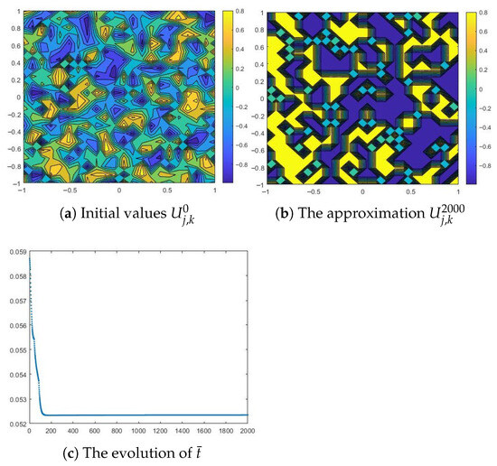
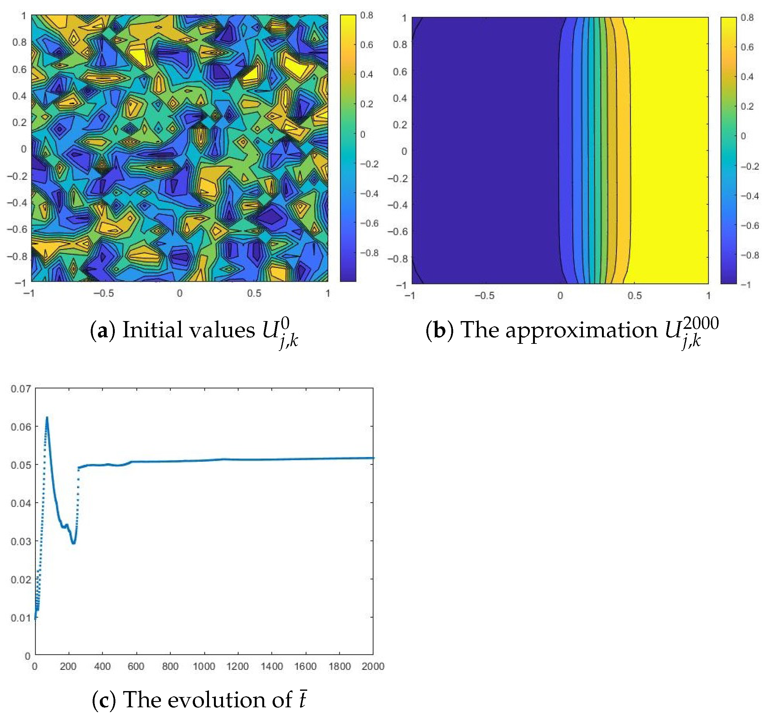
We consider the initial data $u_0$ a square lattice with uniformly random generated values between $-1$ (black) and 1 (white) that can simulate a homogeneous alloy with two constituents. Figure 2a represents such an initial condition. We also choose $g(t,x)=0$ and $f(t,x)=0$, $(t,x)\in Q$ to fit the theoretical background in [7].

Figure 2. Numerical results for a small diffusion coefficient $p_d=0.1$ and $p=1,p_r=1,p_s=0$, and $p_t=0$.

The parameters of the mathematical model will now be set as $p_d=0.1,p=1,p_r=1,p_s=0$, and $p_t=0$. With a small diffusion coefficient, the numerical solution settles in time to a heterogeneous state composed of both phases, $+1$ and $-1$ (see Figure 2b below, where $\epsilon =0.1$ and $T\approx 105$). In [7] the author proved that, for a small diffusion parameter, the solution through $u_0$ to the modified problem (1) (according to input data) does not coarsen at all.

In Figure 2c we can see the evolution of $\overline{t}$ during the time iterations. We can observe that the time-step size remains at the same value after a relatively small number of time iterations.

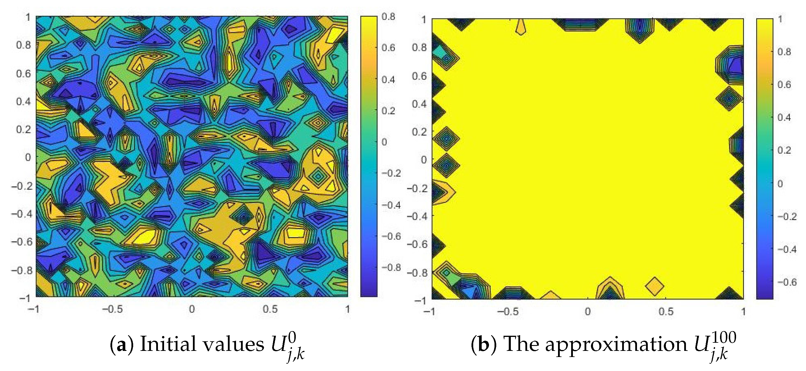
With a large diffusion coefficient, $p_d=5$, and the same values $p_r=1,p=1,p_s=0$, $p_t=0$, we can observe in Figure 3a separation of particles into the two phases, $+1$ and $-1$ (here, $T\approx 98$). As we can see, the initial data changes sign, having large regions of positive sign interposed with large regions of negative sign. After some time, a solution with large regions in which $u\approx +1$ or $u\approx -1$ is formed. These regions are connected by some interfaces, called transition layers.

Figure 3. Numerical results for a large diffusion coefficient $p_d=5$ and $p_r=1,p=1,p_s=0$, and $p_t=0$.

On the other hand, we can see in Figure 4 the approximation of $u(148,x,y)$ for a larger time. We can conclude that the numerical solution to the nonlocal model is attracted to a steady state $(+1)$ for $t\to \infty$.

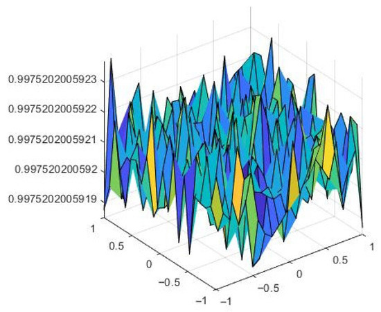
Figure 4. The approximation $U_{j,k}^{3000}$.

All these results are consistent with those in [2,7,11], since it has been proved that, for a large enough diffusion coefficient, the solutions to particular forms of problem (1) do coarsen to either $u\equiv -1$ or $u\equiv 1$. The results of this experiment allow us to conclude that the approximate solution obtained by applying the proposed numerical method is sufficiently accurate.

Experiment 2.

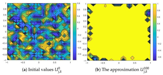
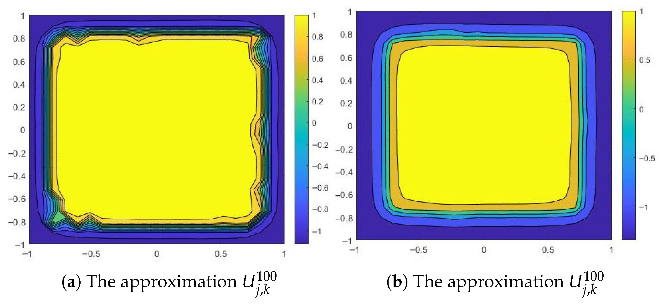
We consider $g(t,x)=-1$, $f(t,x)=1$, $(t,x)\in Q$, and $p_d=0.1,p=1,p_r=2,p_s=1$, and $p_t=0.5$. As we can observe in Figure 5, even with a small diffusion coefficient, the numerical solution is attracted to a steady state $(+1)$ ($T\approx 3.5$). The points near the boundary are an exception. Here, the solution tends to approach the value $-1$, and then, as we move away from the boundary, it tends to $+1$. This is the effect of the Robin boundary conditions embedded in the surface integral term.

Figure 5. Numerical results for a small diffusion coefficient: $p_d=0.1$ and $p_r=2,p=1,p_s=1$, and $p_t=0.5$.

We can draw the same conclusion for a larger diffusion coefficient, $p_d=0.75$ or $p_d=2$. We can observe that the numerical solution is attracted to $+1$, one of the steady states, as time increases (except the points near the boundary) (see Figure 6).

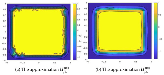
Figure 6. Numerical results for $p_d=0.75$ and $p_d=2$.

We can also observe that starting with $u_0$ bounded, $-1\le u_0\le 1$, the obtained numerical solution remains bounded as it evolves in time. This is consistent with the central result of Section 2. In conclusion, adjusting the size of the time-step at each iteration gives stability to the proposed numerical scheme.

Another interest related to our numerical experiments was to estimate the order of convergence of Newton’s method. This method is based on the fact that, as the sequence of iterations converges, the difference between two successive approximations becomes a good approximation for the approximation error. We used a formula for estimating the convergence order p based on four successive iterations $U^{1,n-2},U^{1,n-1},U^{1,n}$, and $U^{1,n+1}$:

$$p^n={\displaystyle \frac{log(\parallel U^{1,n+1}-U^{1,n}\parallel /\parallel U^{1,n}-U^{1,n-1}\parallel )}{log(\parallel U^{1,n}-U^{1,n-1}\parallel /\parallel U^{1,n-1}-U^{1,n-2}\parallel )}}.$$

For each input data set, we obtained the same thing, namely that the calculated values for $p^n$ quickly tend towards 1, which means that the convergence order of the numerical method is linear.

5. Conclusions

The aim of this paper was to introduce a numerical method in order to approximate the solution to the reaction–diffusion problem (1) with nonlocal diffusion and a nonlinear reaction term. The model can be seen to be similar to the reaction–diffusion Equation (5) with Robin boundary conditions. The boundary conditions of Robin type are somehow incorporated in the second integral term of (1). Using the finite difference method, we have derived a semi-implicit numerical scheme to approximate the solution of the studied model. We have used the Newton method to solve the corresponding implicit problem. The novelty brought by this paper is that we developed an adaptive time-step size numerical method, which ensures the stability of the corresponding numerical scheme. We believe that the numerical method we have proposed is superior in terms of stability and accuracy to the explicit counterpart. The fact that it is a semi-implicit method and that the nonlinear reaction term is treated appropriately, involving the solution at the current time level and not the one at the previous level, makes the provided numerical approximation more reliable. The numerical method uses an adaptive time grid, which means more than a non-equidistant one, because the new time-step size is determined according to several factors, as suggested by Formula (6) and Remark 2, including the initial condition, which changes for each time interval.

As for further directions we intend to use some numerical approaches based on fractional step schemes (as in [17,18,19,20,21,22,23]) and to make some eloquent and comparative numerical experiments. The motivation for such a study is that Newton’s method is an iterative method, while the fractional step method does not require iterations to advance from one time level to another. Therefore, we expect the fractional step method to be faster, which would definitely be a plus. We also want to extend the use of the adaptive time-step mesh obtained on theoretical bases for the nonlocal model to the local model and then compare the results. An important research direction that we are considering for future work is to apply the obtained numerical schemes to real-world problems, such as those in medicine and computer vision [24].

References

- Croitoru, A.; Moroşanu, C. On the existence and numerical approximation of a nonlocal and nonlinear second-order boundary value problem with in-homogeneous Cauchy-Newmann boundary condition. Case 2D. Discret. Contin. Dyn. Syst.-S 2005. [Google Scholar] [CrossRef]
- Bates, P.W.; Brown, S.; Han, J. Numerical analysis for a nonlocal Allen-Cahn equation. Int. J. Numer. Anal. Model. 2009, 6, 33–49. [Google Scholar]
- Bogoya, M.; Gómez, J. On a nonlocal diffusion model with Neumann boundary conditions. Nonlinear Anal. 2012, 75, 3198–3209. [Google Scholar] [CrossRef]
- Miranville, A. Some mathematical models in phase transition. Discret. Contin. Dyn. Syst.-S 2014, 7, 271–306. [Google Scholar] [CrossRef]
- Miranville, A.; Moroşanu, C. Qualitative and Quantitative Analysis for the Mathematical Models of Phase Separation and Transition. Aplications; American Institute of Mathematical Sciences, Differential Equations & Dynamical Systems: Springfield, IL, USA, 2020; Volume 7, Available online: https://www.aimsciences.org/fileAIMS/cms/news/info/28df2b3d-ffac-4598-a89b-9494392d1394.pdf (accessed on 1 October 2024).
- Moroşanu, C. Analysis and Optimal Control of Phase-Field Transition System: Fractional Steps Methods; Bentham Science Publishers: Oak Park, IL, USA, 2012. [Google Scholar] [CrossRef]
- Stoleriu, I. Non-local models for solid-solid phase transitions. ROMAI J. 2011, 7, 157–170. [Google Scholar]
- Croitoru, A.; Moroşanu, C.; Tănase, G. Well-posedness and numerical simulations of an anisotropic reaction-diffusion model in case 2D. J. Appl. Anal. Comput. 2021, 11, 2258–2278. [Google Scholar] [CrossRef] [PubMed]
- Moroşanu, C.; Pavăl, S. Rigorous Mathematical Investigation of a Nonlocal and Nonlinear Second-Order Anisotropic Reaction-Diffusion Model: Applications on Image Segmentation. Mathematics 2021, 9, 91. [Google Scholar] [CrossRef]
- Moroşanu, C.; Satco, B. Qualitative and quantitative analysis for a nonlocal and nonlinear reaction-diffusion problem with in-homogeneous Neumann boundary conditions. Discret. Contin. Dyn. Syst.-S 2013, 16, 1–15. [Google Scholar] [CrossRef]
- Moşneagu, A.-M. On some local and nonlocal reaction-diffusion models with Robin boundary conditions. Discret. Contin. Dyn. Syst.-S 2023, 16, 104–125. [Google Scholar] [CrossRef]
- Moşneagu, A.-M.; Stoleriu, I. An adaptive time-step method for a nonlocal version of the Allen-Cahn equation. Discret. Contin. Dyn. Syst.-S 2024. [Google Scholar] [CrossRef]
- Pérez-Llanos, M.; Rossi, J.D. Blow-up for a non-local diffusion problem with Neumann boundary conditions and a reaction term. Nonlinear Anal. 2009, 70, 1629–1636. [Google Scholar] [CrossRef]
- Banerjee, M.; Kuznetsov, M.; Udovenko, O.; Volpert, V. Nonlocal Reaction–Diffusion Equations in Biomedical Applications. Acta Biotheor. 2022, 70, 12. [Google Scholar] [CrossRef]
- Barbu, T.; Miranville, A.; Moroşanu, C. On a Local and Nonlocal Second-Order Boundary Value Problem with In-Homogeneous Cauchy–Neumann Boundary Conditions. Applications in Engineering and Industry. Mathematics 2024, 12, 2050. [Google Scholar] [CrossRef]
- Croitoru, A.; Tănase, G. On a nonlocal and nonlinear second-order anisotropic reaction-diffusion model with in-homogeneous Neumann boundary conditions. Discret. Contin. Dyn. Syst.-S 2023, 16, 75–88. [Google Scholar] [CrossRef]
- Miranville, A.; Moroşanu, C. Analysis of an iterative scheme of fractional steps type associated to the nonlinear phase-field equation with non-homogeneous dynamic boundary conditions. Discret. Contin. Dyn. Syst. Ser.-S 2016, 9, 537–556. [Google Scholar] [CrossRef]
- Croitoru, A.; Moroşanu, C. Analysis of an iterative scheme of fractional steps type associated to the phase-field equation endowed with a general nonlinearity and Cauchy-Neumann boundary conditions. J. Math. Anal. Appl. 2015, 425, 1225–1239. [Google Scholar] [CrossRef]
- Fetecău, C.; Moroşanu, C. Fractional Step Scheme to Approximate a Non-Linear Second-Order Reaction–Diffusion Problem with Inhomogeneous Dynamic Boundary Conditions. Axioms 2023, 12, 406. [Google Scholar] [CrossRef]
- Fetecău, C.; Moroşanu, C.; Stoicescu, D.C. Fractional Steps Scheme to Approximate the Phase Field Transittion System Endowed with Inhomogeneous/Homogeneous Cauchy-Neumann/Neumann Boundary Conditions. Axioms 2023, 12, 1098. [Google Scholar] [CrossRef]
- Fetecău, C.; Moroşanu, C.; Pavăl, S.D. On the Convergence of an Approximation Scheme of Fractional-Step Type, Associated to a Nonlinear Second-Order System with Coupled In-Homogeneous Dynamic Boundary Conditions. Axioms 2024, 13, 286. [Google Scholar] [CrossRef]
- Moşneagu, A.-M.; Tănase, G. A second-order fractional-steps method to approximate a nonlinear reaction-diffusion equation with non-homogeneous Robin boundary conditions. Discret. Contin. Dyn. Syst.-S 2025. [Google Scholar] [CrossRef]
- Tănase, G. A first-order fractional–steps–type method to approximate a nonlinear reaction–diffusion equation with homogeneous Cauchy–Neumann boundary conditions. Discret. Contin. Dyn. Syst.-S 2024, 18, 566–577. [Google Scholar] [CrossRef]
- Barbu, T. Deep learning-based multiple moving vehicle detection and tracking using a nonlinear fourth-order reaction-diffusion based multi-scale video object analysis. Discret. Contin. Dyn. Syst.-S AIMS J. 2023, 16, 16–32. [Google Scholar] [CrossRef]
Disclaimer/Publisher’s Note: The statements, opinions and data contained in all publications are solely those of the individual author(s) and contributor(s) and not of MDPI and/or the editor(s). MDPI and/or the editor(s) disclaim responsibility for any injury to people or property resulting from any ideas, methods, instructions or products referred to in the content. |
© 2025 by the authors. Licensee MDPI, Basel, Switzerland. This article is an open access article distributed under the terms and conditions of the Creative Commons Attribution (CC BY) license (https://creativecommons.org/licenses/by/4.0/).