Abstract
The crisis of pension systems based on pay-as-you-go (PAYG) financing has led to the introduction in some countries, including Italy, of so-called notional defined contribution (NDC) pension accounts. These systems mimic the functioning of defined contribution systems in benefit calculations while remaining based on PAYG financing. Despite many appealing features, NDC accounts cannot automatically guarantee a system’s financial sustainability in the presence of demographic or economic fluctuations. The literature proposes automatic balance mechanisms (ABMs) of the notional rate applied to notional accounts and an indexation rate applied to pensions. ABMs may be based on two indicators: the liquidity ratio or the solvency ratio. Such ABMs may strengthen a system’s financial sustainability but may produce significant fluctuations in the adjusted notional rate, thereby undermining the social adequacy of the system. In this work, we introduce a mixed ABM based on both the liquidity ratio and solvency ratio and identify the optimal combination that guarantees financial sustainability of the system and, at the same time, maximizes the return paid to the participants at fixed levels of confidence. The numerical results show the advantages of a mixed mechanism over those based on a single indicator. Indeed, although the results depend on the system’s initial conditions and the different ABM configurations tested (16 in total), some common patterns emerge across the solutions. A solvency ratio-based ABM maximizes social utility, while a liquidity ratio-based one ensures financial stability. Although not optimal for either criterion, the ABM that mixes the liquidity ratio and solvency ratio in proportions ranging from 60–40% to 50–50% emerges from our numerical simulations as the best compromise to achieve these two objectives jointly.
Keywords:
notional defined contribution pension systems; automatic balance mechanisms; financial sustainability MSC:
90B50; 90C29; 91B15; 91G05
1. Introduction
Public pension systems financed on a pay-as-you-go (PAYG) basis have historically adopted a defined benefit (DB) architecture to guarantee preset benefit levels and foster a form of intergenerational solidarity. However, population aging and low fertility have eroded the financial sustainability margins of these schemes over time, ushering in a period of reforms. In particular, in recent decades, notional defined contribution (NDC) systems financed on a PAYG basis have established themselves as a credible alternative to traditional DB-PAYG schemes, thanks to the explicit link between contributions paid and benefits received, while maintaining PAYG financing.
In an NDC scheme, individual contributions are credited to virtual accounts that accrue at a notional rate. At retirement, the balance is converted into a life annuity using a conversion factor that reflects the cohort’s expected longevity [1]. The formal structure is of the DC type, but financing remains PAYG; the accounts are not invested in market assets [2]. Thanks to the link between benefits paid and contributions paid, as well as the application of actuarial fairness principles in determining the annuity conversion factor, the DC architecture implicitly promises better financial sustainability of the system, as well as compliance with the principle of actuarial fairness at the individual level [3].
Analytically, the sustainability of a PAYG-NDC scheme is assessed along three interrelated dimensions: liquidity, solvency, and adequacy or fairness. Liquidity concerns the instantaneous balance between current contributions and pension outlays; solvency relates to the intertemporal coverage of liabilities through assets (including the “implicit” PAYG asset) and the dynamics of the buffer fund; and adequacy or fairness considers the actuarial link between contributions paid and benefits, as well as the system’s ability to guarantee minimum levels of well-being [4,5]. From an operational research perspective, Godínez-Olivares et al. [6] proposed a multi-constraint framework that jointly integrates the liquidity and solvency objectives. They formalized PAYG sustainability as a control problem with explicit constraints on intertemporal balances.
1.1. ABMs in the Contemporary Literature
In a stationary regime, an NDC that credits accounts with a “canonical rate” equal to the growth of the wage bill may be in equilibrium. However, in the presence of realistic demographic and economic dynamics, the DC structure alone is not sufficient to guarantee financial balance without adjustments to the rules [7,8].
To address this instability, the literature has developed automatic balancing mechanisms (ABMs) that, when deviations occur, predetermine changes in specific system parameters (notional rate, indexation of pensions, retirement age, and sometimes even the contribution rate) to bring the system back within the liquidity and solvency constraints, avoiding discretionary legislative intervention [9,10]. In international practice, the Swedish case serves as a historical reference; the ABM intervenes annually in the notional rate and pension indexation, based on indicators of the balance sheet position, to preserve the financial stability of the system as a whole [11]. At the theoretical level, ABMs can be classified according to their activation metric: “liquidity-based” mechanisms, which react to deviations between contributions and expenditures, and “solvency-based” mechanisms, grounded in balance sheet aggregates and the relationship between the system’s assets and liabilities [10,12].
On the methodological front, two main research strands have been explored in the literature. The first, the ex-post corrective strand, based on a stochastic approach, studies the effectiveness of ABMs that act on indexation or the notional rate in the face of demographic and macroeconomic uncertainty [10]. In this context, although in a general PAYG framework, the authors of [6] formulated ABMs via multi-objective optimization subject to smoothness (graduality of adjustments) and realism (limits on changes), showing how such constraints reduce the volatility and cyclicity of corrections. In the NDC-PAYG setting, the authors of [12] compared “liquidity ratio” and “solvency ratio” ABMs in a framework with four overlapping generations, measuring not only the stabilizing capacity but also the risk–return trade-off (using Sharpe-style indicators), and they found on average more favorable performance from the solvency-driven mechanisms, albeit with different volatility profiles for the buffer fund. A second strand, concerning ex-ante design, seeks in a deterministic context combinations of parameters that, by construction, generate desired profiles of liquidity and solvency. In this vein lies an overlapping-generations continuous-time model that, with parsimonious assumptions, identifies the conditions for account revaluation rates and annuity indexation needed to obtain liquidity and solvency jointly while also assessing the effects on adequacy and fairness. The mechanisms suggested operate de facto as endogenous, design-stage ABMs [13].
One key aspect is the adequacy of benefits, which must also be analyzed by taking into account the distribution of risks between generations. Most NDC applications keep the contribution rate constant, concentrating adjustments on the benefit side. This choice may preserve the DC “purity” but exposes the system to adequacy risks in aging societies [3]. A recent line of research has integrated adequacy constraints into the design of automatic rules. The authors of [14] proposed ABMs that expand the set of levers to include, in addition to indexation and the notional rate, contributions as well, with regularity constraints and upper and lower bounds in a nonlinear optimization framework that maximizes social adequacy, subject to liquidity and financial sustainability constraints measured over multi-year horizons, showing how multiple objectives can be pursued through combined levers.
Overall, the state of the art suggests the following: (1) NDCs provide an actuarial link between contribution effort and benefits, but they are not self-balancing in dynamic scenarios without appropriate adjustment rules [3,8]; (2) ABMs are the preferred response in variants that emphasize flows (liquidity) or stocks (solvency) [9,11]; (3) solvency-driven ABMs (focused on the PAYG asset and on stocks) may dominate purely liquidity-driven rules (focused on flows) in a risk–return sense at the cost of greater institutional complexity [12]; (4) the explicit adoption of smoothness and realism constraints on lever adjustments (indexation, contributions, and retirement age) improves stability and reduces the oscillation of benefits and balances, as shown in [6] and confirmed in recent NDC applications [14]; and (5) the inclusion of adequacy constraints calls for multi-objective design [14]. Two recurrent limitations remain: on the one hand, the use of deterministic models that abstract from uncertainty [13], and on the other, “toy” stochastic environments (few overlapping generations) that do not fully capture the heterogeneity and joint dynamics of demography, wages, and participation.
1.2. Aim and Scope of This Work
This work addresses the gap mentioned above by undertaking a broad, systematic comparative assessment of automatic balancing mechanism (ABM) families for NDC–PAYG systems within a realistic stochastic environment. We propose a hybrid rule that combines liquidity ratio and solvency ratio activation criteria, which were both introduced in the literature [12], to leverage their complementary stabilizing properties rather than treating them as competing designs. On the one hand, the liquidity-driven ABM [10,12] aims to maintain short-term cash flow equilibrium (i.e., contributions equal to pensions) by acting on pension indexation or on the notional rate. It has some advantages—simplicity, immediacy of imbalance detection, and suitability for short-term shocks—but also several drawbacks. It is a purely cross-sectional criterion that ignores future commitments and therefore does not guarantee intertemporal sustainability. Moreover, in dynamic demographic or economic settings, it tends to increase the volatility of the notional rate and deteriorate the system’s risk–return profile (i.e., lower Sharpe ratio [12]). It also fails to ensure actuarial fairness, since a liquidity correction may alter accrued entitlements. On the other hand, the solvency-driven ABM employs an actuarial balance sheet approach that equates assets (the buffer fund and the contribution asset) and liabilities. This approach’s strength lies in its longitudinal perspective, which assesses the overall soundness of the system and the consistency of accrued rights. It reduces the variance in the notional rate and maximizes the return-to-variability ratio [12]. However, the solvency ratio-based ABM also presents limitations; it can be insufficiently reactive to short-term liquidity imbalances and, when implemented asymmetrically—as in the Swedish case—tends to accumulate excessive reserves, lowering average returns and introducing political rigidity. Neither of the two criteria, in isolation, ensures simultaneous cash flow stability, intergenerational consistency, and robustness to demographic shocks. In [13], the authors showed (in a deterministic, ex ante framework) that combining the two rules yields a system that is “automatically liquid and solvent” in both the short and long run. This solution preserves actuarial fairness and limits reserve accumulation, resulting in a more transparent and stable mechanism. The mixed ABM we propose integrates both ratios into a unified dynamic rule, allowing the system to adjust automatically to demographic and macroeconomic shocks while remaining both liquid and solvent. Formally, it defines the notional rate as a weighted function of the liquidity and solvency ratios, complemented by a dampening mechanism to ensure smooth corrections. This framework, therefore, addresses a problem that has not been previously solved, namely how to reconcile flow and stock equilibrium in a stochastic NDC environment without relying on ad hoc or sequential adjustments. By optimizing the balance between liquidity and solvency targets, the mixed ABM achieves joint minimization of volatility and tail risk for both the notional rate and the reserve fund, thereby linking short-term financial feasibility with long-term sustainability, a feature that no previous single-ratio ABM could guarantee.
The performance of the resulting hybrid ABM is then examined through its application to a stochastic model featuring a realistic population structure, which is calibrated on Italian data. In our model, demographic and economic processes co-evolve, allowing trends to propagate jointly and determine inflows of contributions and outflows of pensions, thus providing a test bed for each rule’s ability to maintain discipline over time.
1.3. Comparison with Alternative Approaches in the Literature
In the broader literature on pension system projections, the approach developed in this study extends the actuarial accounting tradition in a stochastic and dynamic way. Unlike microsimulation models [15,16,17], which simulate individual life courses to evaluate distributional and adequacy outcomes, our framework operates at a more aggregated level. It treats the pension system as a stochastic actuarial balance centered on macro-financial sustainability rather than individual heterogeneity. The model is conceptually related to actuarial accounting frameworks used in NDC balance sheet analyses [11,12]. Nevertheless, it extends them by incorporating stochastic demographic and economic processes in a realistic macro demographic context, moving beyond the simplified overlapping generations (OLG)-type settings commonly adopted in the literature. Compared with OLG models [18,19,20], the proposed approach does not solve for an economy-wide general equilibrium between households and firms. Instead, it preserves an intertemporal and intergenerational perspective by explicitly modeling the actuarial balance sheet of the PAYG–NDC system. Its stochastic structure enables the analysis of uncertainty and distributional risk, which deterministic OLG frameworks and policy microsimulation models cannot capture. Relative to computable general equilibrium frameworks (e.g., [21]), our model is more compact and actuarially grounded, concentrating on the internal consistency of the pension system rather than on full-economy feedbacks. Similarly, while internal rate of return-based studies [5] estimate implicit returns and fairness, they do not model the joint stochastic evolution of the PAYG balance sheet. The present framework embeds that concept within a dynamic simulation, translating the implicit return into a continuous notional rate governed by liquidity and solvency conditions. In addition, our framework is consistent with the institutional approaches promoted by the World Bank [22] and the OECD [23], which emphasize automatic stabilizers, transparent accounting, and the balance between adequacy and sustainability.
A central aspect of the analysis is to highlight and measure the trade-offs that arise between short-term cash flow stability, the longer-term balance sheet position, and adequacy of benefits. To ensure that these comparisons are valid for policy implementation rather than abstract optimality, we adopt a multi-criteria assessment consistent with the smoothness and realism constraints highlighted in prior work [6,14]. Concretely, the assessment framework is built to compare liquidity-driven and solvency-driven ABMs under a range of regulatory configurations aligned with the NDC architecture and the Italian demographic-economic context, while enforcing gradual adjustments and plausible bounds on policy levers. Within this framework, we track how different design choices perform when targets (liquidity versus solvency) are prioritized, which levers are activated (indexation and the notional rate), whether the adjustment rule is symmetric or asymmetric, whether the statutory retirement age is allowed to adapt, and whether a survivor dividend is distributed. We also quantify the combined implications of these choices for adequacy and actuarial fairness. Together, these elements give rise to design and evaluation criteria that help identify ABM models that remain effective, efficient, and transparent, demonstrating robustness to macro-demographic fluctuations and consistency with the social and financial constraints.
1.4. Organization of the Paper
The work is organized as follows. Section 2 outlines the pension system specifications, defines the stochastic dynamics of the considered sources of uncertainty, and introduces the two ratios needed later to define the ABMs. Section 3 defines the classic liquidity- and solvency-based ABMs, generalizes them to the mixed ABM proposed in this work, and defines all the optimization problems that must be solved jointly to find the suboptimal ABM that guarantees improvements for both the social utility and financial sustainability of the considered pension system. Section 4 presents our numerical results, both discussing a specific optimization problem in detail and providing an overview of the cases when mixed ABMs must be preferred over the classic ones. Finally, Section 5 summarizes the results obtained in this work and discusses related open problems that are worth investigating in future research papers.
2. Time Evolution of the NDC Account
In this section, we describe the considered NDC pension system. Section 2.1 presents the financial structure of the model and the main assumptions. Section 2.2 introduces the assumptions needed to specify the dynamics of the underlying risk factors. Further specifications are provided in Section 4, where the model calibration and parameterization are reported.
2.1. Model Definitions and Structure
Let , , and be the number of individuals, contributors, and pensioners of age x at time t, respectively. The demographic structure at any time t is represented as follows:
We consider individuals as potential contributors since a given age , which is the first explicitly represented in the model. Furthermore, the system is assumed to be closed to migration, and hence depends only on the number of newborns in alive by t. This assumption is taken into account by introducing the rate , which is fully specified later in Section 4.1. Furthermore, assuming no migration, the population () evolves for the mortality contribution only. Hence, it holds that
where is the time-dependent 1-year survival probability (i.e., the probability that an individual of age by time will reach age x by time t).
The contributors’ dynamics are described by the employment-to-population ratio per age :
which is assumed to take the form . Furthermore, let us also consider the overall employment-to-population ratio:
where is the retirement age. The variables and are fully specified later in Section 4.1, while, by construction, can be expressed as follows:
The average individual salary per contributor of age x by time t is assumed to take the form
Hence, we have
which represents the total salary amount with t, and
are the average individual contribution and the overall contribution at time t, respectively, where is the fixed contribution rate of the NDC pension scheme.
The notional rate for the period is evaluated according to the canonical NDC approach [7]:
The notional pension wealth is calculated for each cohort based on the contribution pattern of the individuals belonging to that cohort. Two alternative definitions are proposed:
where is the cohort pension. The definition in Equation (9) accounts for the accumulation of contributions and their revaluation based solely on the notional rate . Meanwhile, Equation (10) also takes into account demographic effects, namely the redistribution among survivors of the notional amounts of deceased individuals, or the so-called survivor dividend [24]. Both Equations (9) and (10) are alternatively considered in our numerical results, although only the notation is used in the rest of this section for the sake of brevity.
At retirement age , the cohort pension is evaluated as follows:
where the life annuity is defined as
with and being the pension indexation and the probability at t of an individual of an age x to survive up to age , respectively. From an operational point of view, pension indexation is implemented via tying the benefit to an economic indicator, typically inflation or the salary growth rate. In the following numerical application, we assume that pensions are indexed to the inflation rate (), consistent with Italian legislation [14], which serves as our benchmark when defining the baseline set of assumptions.
It is worth noting that Equation (12) does not utilize , , or . Instead, is defined as a function of the ex ante estimates , , and . These quantities are conditioned to and thus are affected by an estimation uncertainty that may let them differ from their corresponding ex post measured values. For the sake of simplicity, we assume that is estimated as the 3-year moving geometric average of the corresponding past observations
for each . The same applies to . Furthermore, let
Specifically, the future 1-year survival probability of individuals of an age is estimated at t as the empirical survival rate observed for cohort in t.
The retirement age is unique for a given cohort, although it is also considered a dynamic version:
This may imply different retirement ages for different cohorts. The population of new pensioners
is assumed to be equal to the number of individuals alive at t, regardless of the former employment pattern of each contributor. It is worth noting that this specification is not relevant to our study, as it only affects the average individual pension. On the other hand, the initial cohort pension is independent of the number of new pensioners, as shown in Equation (11). Thus, Equation (16) does not affect the financial sustainability of the considered NDC system.
The number of pensioners and the cohort pension at ages are evaluated as follows:
The financial state of the pension system is summarized by the value of the reserve fund
where
The fund level represents the account balance of all the past cash flows which originated from both contributions and benefits. Two different financial indicators are introduced in the following to assess the fund’s financial adequacy.
The liquidity ratio [12], expressed as
compares the fund’s level against the short-term liabilities that the system is required to pay. While highlights the short-term financial inadequacy of the fund, suggests an inefficiency in the pension system that should be addressed. Thus, is a desirable equilibrium target value.
The medium-to-long-term financial adequacy of the fund is measured by the solvency ratio. This ratio assesses the pension scheme’s solvency by comparing outstanding liabilities to contributors and retirees against the buffer fund and the pay-as-you-go asset (or contribution asset) [13]. While liabilities are derived by actuarial valuation, assets must be estimated, consistent with the unfunded nature of PAYG schemes:
where
quantifies the outstanding liabilities of the pension system at t, while
is the contribution asset. Consistent with the Swedish method balance sheet approach [5], is calculated as the product between the contribution amount and a duration term
Loosely speaking, represents the average time of stay of a unit of value in the pension system. In the medium-to-long term, the interpretation of is the same as in the short term.
2.2. Dynamics of the System’s Risk Factors
As discussed in Section 2.1, the system evolves according to both demographic and economic risk factors. A stochastic multivariate process describes their dynamics. This section introduces all the assumptions needed to specify the time evolution of the considered system. Indeed, there are five risk factors to be modeled: (natality), (survival probability), (employment), (salaries), and (inflation). A realistic description of these factors’ dynamics enables us to simulate the probability distribution at future times and thus compare strategies aiming to preserve the financial stability of the system.
Natality, salaries, inflation, and employment are modeled jointly. Marginal dynamics are chosen according to the respective domains, while the joint distribution is obtained while assuming that the stochasticity generator is a multivariate Wiener process such that
where is the correlation matrix whose elements are equal to the Pearson coefficients (). In addition, , , and are assumed to be properly represented by lognormal marginal dynamics:
Due to its compact domain, the employment-to-partecipation ratio is assumed to obey logit-normal dynamics:
Regarding participants’ mortality, we denote with and the number of deaths and exposure in the population group i at age x in the year t, respectively. We assume that , where is the central death rate at age x and year t for the population group i. The time evolution of mortality is described by the Lee–Carter model, which is considered a benchmark in the literature on mortality modeling [25]. Therefore, the evolution of the central death rates is represented by the following equation:
where is the static age function representing the mortality level at age x, is the mortality time index, and is the non-parametric age-period term measuring the sensitivity of mortality at age x to the time trend. All the parameters refer to the specific population group i. The corresponding death probabilities are derived from
The future mortality evolution is obtained by predicting the time index , which is modeled using an auto-regressive integrated moving average (ARIMA) process. According to the standard literature, we adopt an ARIMA of (0,1,0) for :
where is the drift parameter and are the error terms, which are normally distributed with a null mean and variance , .
In our setting, the Lee–Carter model is calibrated separately by gender (). This choice follows from the features of the historical data considered. However, possible effects of the gender distribution on the other risk factors (e.g., impacts of gender inequality on and ) are beyond the scope of this study, which is devoted specifically to investigating improving the financial sustainability of NDC accounts by introducing a new class of ABMs. Furthermore, the granularity of the dataset chosen to calibrate , , and does not cope with an explicit gender representation (see Section 4 for further details on calibration). Indeed, Equations (1), (17) and (18) consider a gender-free survival probability
that is obtained as a weighted average of the corresponding gender-dependent probabilities, where the weights are evaluated recursively:
The joint dynamics of the demographic factors (i.e., natality and mortality) and economic factors (i.e., employment, salaries, and inflation) provide a full description of all the elements relevant to the proposed pension system, given the assumption of system closure introduced in Section 2.1 above.
3. The “Mixed” ABMs
This section introduces the core concept proposed in this work—the mixed ABM—which generalizes the ABMs based on solvency and liquidity ratios. These two classic ABM forms are summarized in Section 3.1. Section 3.2 defines the mixed ABM in its most general form. A dampening mechanism is then introduced in Section 3.3 to guarantee shock-free dynamics, as in a realistic case of ABM application. As discussed therein, this mechanism allows us to restrict our analysis to a simplified form of the mixed ABM. Finally, Section 3.4 introduces the optimization problems that arise from the purpose of maximizing both the social and financial benefits jointly. Those problems are then investigated numerically in Section 4.
3.1. ABMs Defined over LR and SR
The class of ABM investigated in this work represents a generalization of two specific ABMs already considered in the literature [12,13] that are designed to attain the target conditions and . As discussed in Section 2.1, this level is a desirable break-even point for both indexes to achieve a balance between efficiency and sustainability for the system. In both cases, the ABM drives the system by redefining the notional rate .
Solving Equation (34) for the notional rate leads to
The condition for Equation (22) implies a similar result for the solvency ratio ABM . Indeed, it holds that
The ABMs introduced in both Equations (35) and (36) are defined in “symmetric” form, which means that the correction applied to the rate ( or ) can be less than or greater than one. Alternatively, ABMs can be redefined as “asymmetric”, i.e., assuming that corrections are applied only to reduce the rate. The choice of asymmetric ABMs is made in cases where the system is regulated with the sole objective of protecting its sustainability, without taking into account its efficiency [12,26,27]:
where the ratio can stand for either or .
3.2. The Generalized “Mixed” ABM
Since and share the same functional form, it is possible to introduce the following generalized ABM:
where and under the normalization constraint .
The three-degrees-of-freedom ABM generalizes all the notional rates introduced above: (), (), and (). The parameter is introduced, as a non-normalized parameterization of the weights would not allow for a financial interpretation of the target. Nonetheless, the numerical investigation of the properties of is well posed, provided that at least two weights are not equal to zero or one. Adjusting the weight directly modifies the balance between the liquidity and solvency objectives embedded in the mixed ABM. In our formulation, continuously shifts the system’s sensitivity from solvency- to liquidity-based corrections. When , the mechanism behaves like a pure liquidity-based ABM, reacting strongly to short-term cash flow deviations. This ensures immediate budget balancing but increases volatility in the notional rate and weakens intertemporal consistency. The pension system remains liquid in each period, yet long-term solvency may deteriorate because accumulated liabilities are not fully internalized in the adjustment. When , the mechanism converges to a pure solvency-based ABM, prioritizing balance sheet stability and the preservation of accrued rights. This configuration reduces volatility and improves the Sharpe ratio of the notional rate [12] but responds more slowly to transitory imbalances, potentially generating temporary liquidity gaps. Intermediate values of produce a balance between these two regimes. In short, acts as a policy lever that tunes the degree of reactivity of the ABM where higher weights favor immediate liquidity discipline, lower weights favor long-term solvency preservation, and intermediate values achieve the best overall risk–return balance under demographic and macroeconomic uncertainty.
An overall simplified schematic of the interaction between the ABM and the pension system is displayed in Figure 1.
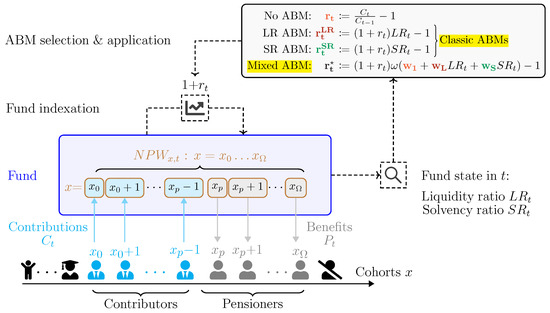
Figure 1.
Simplified schematics of the interaction between the pension system and the ABM at a given time instant t. Only the symmetric ABMs are displayed for the sake of readability.
The same generalization is possible in the asymmetric case as well:
given the same domain and constraints introduced for . Hence, an ABM in our framework is uniquely identified by the parameter set
where a is the Boolean variable that specifies whether the considered ABM is symmetric.
3.3. The Dampening Mechanism
It is worth noting that the annual application of ABM implies the need for a smooth variation in the resulting notional rate to prevent jumps in its path and guarantee its social sustainability [6]. To cope with this requirement, we choose to introduce a dampening mechanism in our numerical set-up by bounding and as follows when applying the ABM:
The same mechanism is applied to the generalized asymmetric case as well.
The choice of guaranteeing the smoothness of the ABM dynamics through the dampening mechanism introduced above allows for some simplifications concerning the parameter set that defines the mixed ABM itself. Indeed, the local effects of or are inhibited by a restrictive enough choice for the parameter . Furthermore, the weight plays a role similar to the dampening mechanism introduced above, as it reduces the ABM sensitivity to and . In fact, the case is equivalent to removing the ABM from the system by construction.
As all our numerical simulations implement stabilization of the pension system through the substitutions reported in Equation (41), we choose to reduce the mixed ABM by imposing . In the process, Equations (38) and (39) are simplified as follows:
given that the dampening mechanism introduced above implies that only one degree of freedom is worth being optimized. This simplification aligns with intuition, as we have eliminated two degrees of freedom by introducing two-parameter damping of the dynamics.
3.4. Optimality Criteria
Generally speaking, the introduction of an ABM forces legislators to choose between two conflicting objectives: improving the financial sustainability of the system on the one hand and, on the other, ensuring its social utility. The choice of one or both of these targets drove the choice for the optimality criterion in several recent works on this topic [6,12,14].
This work aims to verify whether nontrivial parameterization (i.e., ) of the mixed ABM may be an optimal choice concerning both the social and financial aspects of the pension system. The population of contributors and pensioners modeled in Section 2 is affected by demographic and economic uncertainty, which also has consequences in terms of solvency and efficiency of the fund underlying the pension system. Thus, unlike other former studies on ABMs and their effects, the problem we aim to address is not limited to optimizing a deterministic dynamic of the considered system. Conversely, we are considering the distribution of system states reached at each future observation time t and require that the mixed ABM can achieve “likely” stabilization of the pension system in most scenarios generated by the risk drivers’ stochastic dynamics over the years.
To this end, we consider two variables that quantify the financial sustainability and social utility of the system. Based on each of them, a set of cost functions is then introduced, taking into account their distributions for each simulated t and each considered ABM setting, with the latter being specified by the couple . The cost functions to be optimized are defined based on the one-parameter family of distributions that describe each variable as the system evolves stochastically.
To take into account the degree of social utility, we choose to consider the notional rate together with a selection of its statistics. Since is applied equally for each cohort, the social utility and efficiency of the system for a given ABM can be evaluated without explicitly considering the population distribution across ages. The statistics chosen for this purpose are
where is the expected value of a function of a random variable evaluated over the random variable’s sample space. In this case, is the expected functional value evaluated over the notional rate distribution in t. The Sharpe ratio “”, as a risk-adjusted measure of the notional rate , has already been utilized in the literature to evaluate the social utility of a pension system [12]. It is worth noting that the notional rate distribution in t is always conditioned by the chosen ABM configuration , which is kept fixed as the system evolves over time t and across all the risk factors of the simulated scenarios.
For social purposes, the trajectory should be as high and stable (i.e., not volatile) as possible. Thus, we consider the two following objective functions, based on the statistics defined in Equations (44) and (45):
where t is considered from the first simulated year up to a given projection horizon . Namely, as we aim to keep as stable as possible across all the scenarios and through all the life span of the individuals belonging to the considered population, we evaluate the maximum volatility and minimum Sharpe Ratio —evaluated across the scenarios—through all the simulated years, given a fixed value that specifies the mixed ABM.
Then, we can numerically minimize and maximize in the ABM parameter space by solving the following optimization problems:
having fixed (i.e., the optimization is performed separately for the symmetric and asymmetric ABMs). If both solutions and are remarkably far from the dominion boundaries zero and one—and hopefully —then the mixed ABM is shown to be a clear enhancement of the classic LR and SR ABMs in terms of social effectiveness of the considered pension system.
A similar approach is followed in optimizing the mixed ABM concerning the system’s financial sustainability. In this case, the fund value is directly considered an expression of the system’s solvency. Similar to the case regarding social utility, we also aim to maintain a high and stable to ensure financial sustainability. Nonetheless, too high of an level would be a clear symptom of inefficiency and thus not desirable. Instead, we choose to set a criterion inspired by the regulatory approach established for European banks and insurance companies by the regulatory frameworks “Basel” and “Solvency”, which evaluate the financial sustainability of a firm through a value-at-risk measure, specifically considering a given profit-and-loss-distribution quantile associated with a worst-case scenario of loss. This approach cannot be replicated literally in our ABM calibration, as a country can finance its welfare system through taxes (while a bank cannot), and the financial resources available are not to be interpreted as a capital at risk that makes sense to compare with an absolute loss level. Nonetheless, considering a quantile of the distribution instead of an absolute level is a good choice in this context as well. For example, the condition would prevent a country from borrowing financial resources to pursue the best interest of its population, which is in evident contrast with the real-world practices. Conversely, trying to maximize the level occurring in a worst-case scenario forces all the profit and loss distribution upward without any hard constraint, which may contrast with realism.
That said, the statistics chosen for this purpose are
where is the cumulative density function of . The standard deviation also remains a good indicator of the (absence of) stability from the financial perspective, and thus it is maintained. In analogy with Equations (46) and (47), we introduce the objective functions
The optimization of these two functions is achieved by solving the following two problems:
4. Numerical Specifications and Results
This section outlines the effects of mixed ABMs introduced in Section 3 on the dynamics of the pension system presented in Section 2.
The reference context and the historical datasets utilized in our numerical simulations are those of the Italian population and pension system. Indeed, Italy provides a particularly relevant case study for analyzing the performance of NDC–PAYG pension systems. It was one of the first countries—together with Sweden—to introduce a notional defined contribution architecture through the Dini reform (Law 335/1995), which replaced the previous earnings-related defined benefit scheme with a contribution-based formula while maintaining PAYG financing. The reform established notional individual accounts, automatic adjustments through annuity conversion factors linked to cohort life expectancy, and a gradual transition for pre-1996 cohorts [7,28]. Subsequent reforms further strengthened the system’s financial sustainability. The Fornero reform (Law 214/2011) unified the NDC approach across all workers, accelerated the phasing in of the contribution-based formula, and linked statutory retirement ages and seniority requirements to longevity updates [29]. These adjustments also raised the minimum retirement age, tightened access to early pensions, and harmonized contribution rules across sectors. From a demographic and macroeconomic perspective, Italy faces one of the fastest aging processes among OECD countries, with fertility persistently below replacement and a dependency ratio projected to exceed 80% by 2050 [23]. These trends make automatic stabilizers and ABM-type mechanisms particularly relevant. Moreover, the Italian NDC scheme has been the object of extensive academic and institutional study, covering its theoretical foundations, transition design, actuarial fairness, and sustainability assessment [7,23,30,31]. For these reasons, Italy represents a large and data-rich setting in which to test the properties of an ABM under realistic demographic and economic conditions.
The section is organized as follows. The numerical results discussed hereinafter were obtained while considering three distinct sets of initial conditions and assumptions, described in Section 4.1. Two realistic settings are introduced by calibrating the model described in Section 2 using Italian demographic and macroeconomic historical datasets. Indeed, by considering Italian historical data up to 2015 and up to 2024, two dynamics of slowly and rapidly decreasing populations are projected. A third set of a priori conditions is also considered in order to obtain an expected driftless behavior for the system.
In Section 4.2, the settings that imply a slowly decreasing population are projected up to a 150-year time horizon to assess the long-term effect of mixed ABMs and identify a suboptimal parameterization across all the possible configurations, with 100-year and 50-year time horizons considered as well. In Section 4.2.1, a specific configuration is selected among those introduced in Section 4.1 as a case study to show the numerical optimization and application of a mixed ABM to the Italian case, with information filtered up to 2015. Then, Section 4.2.2 provides an overview of the cases when a mixed ABM results in an improvement over the classic - and -based ABMs or otherwise across all the eligible configurations.
Finally, Section 4.3 studies the Italian setting when calibrated with data up to 2024. As this parameterization features a rapid decrease in population, simulations were limited to a 50-year projection horizon. Section 4.3.1 simulates the system under the same configuration previously considered in Section 4.2.1. Subsequently, Section 4.3.2 discusses a sensitivity analysis performed over the main sources of uncertainty in the system.
4.1. Calibration and Initial Conditions
This section introduces the three distinct settings considered in our numerical investigation and the model calibration. As anticipated above, we calibrated the model described in Section 2 using publicly available Italian time series. In the following, in Section 4.1.1, we discuss how specific characteristics of the Italian demography have led us to the introduction of three distinct settings to test the mixed ABM on in simulated pension system based on the Italian historical data. Further details on the model’s parameterization and data sources are available in Section 4.1.2.
4.1.1. Considered Settings
The Italian population is affected by a significant aging issue, and it is characterized by a low natality rate that has been decreasing over time. In fact, calibrating the model through Italian historical data up to 2015 led to a slightly negative estimate of in Equation (27). The pandemic period implies an additional negative impact, increasing the mortality rate across all age groups (compare Table A4, Table A5, Table A6 and Table A7 in Appendix A). In the years following the COVID-19 pandemic, a further decline in natality has been observed (see Table A1 in Appendix A). Thus, calibrated using data up to 2024 was remarkably more negative than the result obtained when calibrating the model with observations limited to 2015, and the expected mortality increased as well.
The model introduced in Section 2 serves as a functional workbench where the applicable ABMs are compared over a distribution of demographic and economic scenarios. Namely, the model aims to return a distribution ranging from highly positive to worst-case scenarios so that ABMs are tested and may reduce volatility and limit the tail of negative scenarios with a certain degree of effectiveness. Conversely, the model does not aim to provide a reliable forecast concerning Italian demography and economy. To this end, several specifics of the Italian system which are not relevant to this work should be included, such as migration phenomena and political actions. It is worth noting that the exclusion of migration is aligned with practices commonly adopted in similar studies in the contemporary literature (see, for example, [6,12,14]). Furthermore, long-term political actions cannot be explicitly modeled in this context.
The top panels in Figure 2 display the projected dynamics for the number of contributors and the number of pensioners , based on a model calibration that considers Italian data up to 31 December 2024. The simulated distribution of the population shrank to zero within a century, causing all the simulated scenarios to collapse into an empty system. It is clear that as the population decreases over time, the role played by immigration and the government’s choices concerning natality grows to assume capital relevance. Indeed, when considering the most recently available data in our simplified framework and projecting the contributor and pensioner distributions up to 150 years, the current situation is taken to an unrealistic extreme, instead of generating the wide range of possible scenarios needed for investigating the effectiveness of the mixed ABM, which is the purpose of this work.
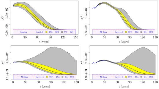
Figure 2.
Number of contributors and number of pensioners simulated over time (150-year-long projection horizon). The pensioner population obeys Equation (15). The distributions per year of observation are displayed through the 5–95 percentile interval (gray areas) and the 25–75 percentile interval (overlapping yellow areas). The central black line represents the median. The red dashed line highlights the zero level. (top panels) The information available to the model, filtered up to 31 December 2024. (bottom panels) The information available to the model, filtered up to 31 December 2015.
For this reason, we considered two distinct Italian set-ups. In the first one, we calibrated all the parameters involved in the dynamics of the risk factors as defined in Section 2.2, considering data truncated to 31 December 2015. The effect of this choice is shown in the bottom panels of Figure 2, where a mild decreasing trend in the expected population can be observed over a 150-year projection horizon, but at the same time, a wide population distribution was maintained across the simulated scenarios through the whole projection horizon considered, coping with the purpose of this work. Indeed, this set-up was used to simulate and compare the effects of various ABMs over a 150-year projection. The second set-up was calibrated using the entire Italian dataset up to 2024. This second choice embedded the current trends in natality and mortality. However, it generated the demographic catastrophe mentioned above over a 100-year-long period, as the model does not consider immigration, political actions, or a possible time evolution of the parameters. Thus, this second set-up was used to simulate and compare the effects of various ABMs over a 50-year projection.
In the following, the two settings described above are referred to as the 2015 and 2024 “Italian” settings. Additionally, a third setting is introduced, which was derived from the 2015 Italian setting through two modifications. First, all trend terms in the dynamics of the risk factors were set to zero while keeping the volatilities and correlations calibrated for the Italian setting unchanged. Second, the system started empty; simulations commenced with , and the population was gradually developed through the dynamics, as limited by the Lee–Carter mortality model. The system evolved stochastically over a century without any ABM applications. ABMs were then introduced and compared, starting from . In this third setting, referred to as “Driftless”, the single set of initial conditions used in the 2015 Italian setting is replaced with a distribution of initial conditions, originating from the trajectories simulated to initialize the system in each scenario. The primary reason for introducing this further configuration of the system was to ensure that the specific characteristics of the Italian settings did not bias any conclusions drawn about the mixed ABMs in our numerical simulations. Since in the Driftless setting, Monte Carlo scenarios were generated over a 150-year-long period, as in the 2015 Italian setting.
4.1.2. Model Calibration and Data Sources
To calibrate the model, we utilized two data sources. In particular, the calibration of the multivariate process jointly describing natality, salaries, inflation, and employment (see Equations (26)–(28)) was achieved through datasets provided by the Italian National Institute of Statistics (ISTAT) [32] (observations available between 1996 and 2024), while the Lee–Carter model, representing the dynamics of mortality (see Equations (29)–(31)), was calibrated based on data extracted from the Human Mortality Database (HMD) [33] concerning the Italian yearly mortality measured per gender between 1975 and 2022. Table A1, Table A2, Table A3, Table A4, Table A5, Table A6 and Table A7 in Appendix A display the calibrated parameters across the three considered settings. Specific references to the time series available from the two data sources mentioned above, used in calibration, are listed in Table A8 in the same appendix.
The same data sources also provided the initial conditions. Indeed, was obtained by applying Equations (32) and (33) to the most recent cross-section among those extracted from the HMD website. Furthermore, distributions per year of observation across all ages are available on the ISTAT website concerning, inter alia, , , and . Thus, follows from Equation (2), and follows from Equation (6) directly. The latter also enabled the computation of through Equation (7) after fixing , which was set to across all the configurations considered in the remainder of this section. Beyond , just a few other quantities were fixed a priori: and , utilized in Equation (15), and and , utilized in Equation (41). If the retirement age was fixed instead of being dynamic, then it was set to 64 years.
To set the initial value, which was not publicly available nor could it be fully inferred from historical data, we chose to approximate the system as stationary during the years . Let us pretend that the pension system is activated in for the cohort . For , the contributions keep accumulating in the notional pension wealth of each cohort before the pension system grants benefits for the first time. During that period, Equation (9) simplifies to
When assuming a stationary demographic structure over the same period
together with constant salary rate and survival probability , we can simplify Equation (56) further, yielding
where the canonical NDC approach introduced in Equation (8) implies under the stationary framework approximation described above. Given , Equation (58) can be applied iteratively until the initial condition is fully determined for all the active cohorts. The same approximation can be applied to compute . Furthermore, by pretending the stationary framework is also valid for the interval , the argument can be easily extended to estimate , completing the set of initial conditions needed.
4.2. Projections up to 150 Years: The “Driftless” Case and the “2015 Italian” Case
In this section, mixed ABMs are tested using the “2015 Italian” and “Driftless” settings. Unlike the “2024 Italian” setting, these parameterizations are not affected by any long-term natality catastrophe. Hence, we could safely simulate projection horizons up to 150 years (i.e., 50-, 100-, and 150-year horizons).
In Section 4.2.1, a specific pension system configuration is considered, and the numerical solutions to the optimization problems in Equations (48)–(55) are thoroughly discussed. In the subsequent section (Section 4.2.2), the optimal solutions to the four problems mentioned above are systematically reviewed across all eight possible pension system configurations, three projection horizons, and both settings.
All the simulated distribution dynamics reported in this section and the next one were generated through a Monte Carlo implementation featuring a number of scenarios ranging between 5000 and 10,000. We verified that our numerical results were already completely stable when simulating at least 2000 scenarios.
4.2.1. A First Example of the Mixed ABM Effect: The 2015 NDC Italian System
The following provides an example of mixed ABM optimization and application before summarizing the results obtained across all tested configurations. Two aspects of what follows are relevant in the context of this work.
First, the case study described below makes clear how the mixed ABM parameterization is far from being a convex optimization problem. In fact, due to the simultaneous optimization of four different objective functions—introduced in Section 3.4—an exact optimal solution does not exist at all. However, considering a fixed tolerance level, a neighborhood of suboptimal solutions can be defined around each of the four optimal values. The intersection among those neighborhoods allows for the identification of a set of suboptimal solutions that may satisfy, to some extent, both the social and financial requirements for optimizing the system.
Second, the results of the Monte Carlo numerical simulations are presented, illustrating how the ABM affected the distributions that define the system’s stochastic dynamics over time.
The simulated configuration adopted the “2015 Italian” setting introduced in Section 4.1. Furthermore, the notional pension wealth was evaluated according to Equation (10), and the retirement age dynamics were governed by Equation (15). The mixed ABM to be optimized was chosen to be symmetric. As the system implements the dampening mechanism introduced in Section 3.3, the ABM takes the form reported in Equation (42). It is important to note that this configuration was chosen arbitrarily, and it does not hold any greater relevance compared with other possible configurations.
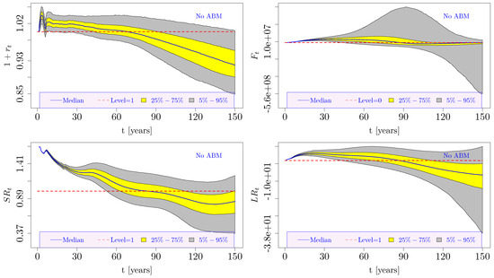
Figure 3 displays the stochastic evolution of , , , and over 150 years in the case of no ABM application. The polyline-like aspect of and in the first simulated years was due to the dynamics of . All four distributions gradually shifted downward in the long term, implying the progressive financial unsustainability of the system. This evolution can be easily explained as originating from demographic risk factors. Indeed, the and dynamics are plotted in Figure 2 (bottom panels), showing a progressive reduction in the median population, although a certain degree of variance was also maintained in the long term across the Monte Carlo simulated scenarios. Note that the increase in the retirement age up to proved insufficient to ensure the system’s financial sustainability (i.e., ). At the same time, the evolution of the demographic and economic factors that affect the contribution base led to .
The best mixed ABM was identified by solving the four optimization problems introduced in Section 3.4. As anticipated above, each of them was solved on three different time horizons: 50, 100, and 150 years.
Figure A1 in Appendix B illustrates the solutions to the two problems aimed at maximizing the system’s social utility (see Equations (46) and (47)). As displayed in the left panels, the strictly optimal solution to minimize was to apply an SR-based ABM to the system (). However, introducing a tolerance (pink areas) showed that the neighborhood of almost-optimal solutions extended deeply into the mixed ABM region. Conversely, the optimal choice to maximize was a mixed ABM with (right panels).
Furthermore, Figure A2 displays the solutions to the two problems aimed at maximizing the financial sustainability of the system (see Equations (54) (left panels) and (55) (right panels)). Considering the tolerance, all six optimizations together suggest that is a suboptimal solution that satisfies all the requirements to some extent. Since this solution is acceptable from both the financial sustainability and social utility perspectives, a mixed ABM was ultimately applied to the system.
The effects of the mixed ABM are displayed in Figure 4.
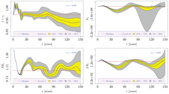
Figure 4.
Simulated dynamics of , , , and (150-year-long projection horizon). The pension system adopted the Italian setting (i.e., historical data were considered up to 2015) and obeyed Equations (10) and (15). A symmetric mixed ABM was applied as defined in Equation (42), where . Color conventions are the same as those utilized in Figure 2 and Figure 3 above.
The median of remained oscillating around zero throughout the considered time horizon, indicating the achieved financial sustainability of the system. The improved trends of and support this result. At the same time, also showed an improvement, implying a more efficient pension system and a social utility improvement as well.
4.2.2. Systematic Results
The NDC pension system discussed thus far comprises several different configurations, each of which possibly leads to a different optimal ABM choice. To better define the scope of the following analysis, we restricted our consideration to the dampening mechanism and the resulting simplified forms of the mixed ABMs introduced in Section 3.3. This choice, also applied in the case study presented above, reduced the dimensionality of the optimization problems related to identifying the best ABM.
As seen in Section 4.2.1, identifying the optimal ABM is a nontrivial task. Indeed, the four optimization problems introduced in Equations (48)–(55) have distinct solutions, implying that a single solution that is optimal for each considered problem does not exist. Thus, we introduced an arbitrary tolerance level to define a neighborhood of suboptimal ABMs around each optimal solution and to identify a “good” suboptimal ABM that approximately satisfied all the considered objective functions (see Figure A1 and Figure A2).
In certain cases, introducing tolerance may not be sufficient to select the proper ABM. Indeed, the four optimal solutions to Equations (48)–(55) may end up being divided between “pure” -based and -based ABMs. Even in this case, a mixed ABM with is likely to be the best compromise, as it preserves both social utility and financial sustainability to some extent, although not optimally in either perspective.
Given the restrictions described thus far, we had 16 distinct configurations generated by the possible combinations of four choices: setting (“2015 Italian” or “Driftless”); retirement age (dynamic or fixed); notional pension wealth (demographic effects neutralized or not); and mixed ABM symmetry (symmetric or not). The case study presented in Section 4.2.1 is one of them, with the “2015 Italian” setting, dynamic , no demographic effects on , which follows Equation (10), and symmetric ABM.
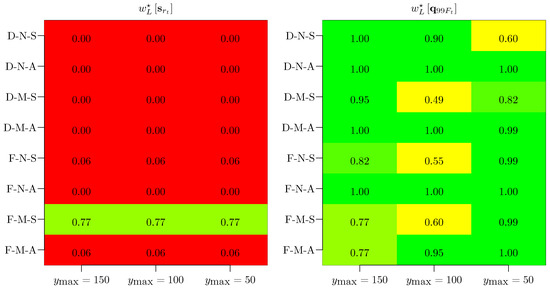
An overview concerning the best ABM choice for each of the remaining 15 configurations is reported in the remainder of this section. For the sake of simplicity, the optimization was limited to the criterion in Equation (49) for social utility and the one in Equation (55) for financial sustainability. The results are summarized in Figure 5 and Figure 6 separately for the “2015 Italian” and the “Driftless” settings.
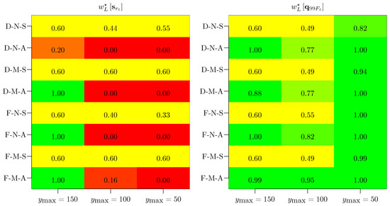
Figure 5.
Optimal solutions for the problems stated in Equation (49) (left panel) and Equation (55) (right panel). When limiting the simulations to the 2015 Italian setting only, eight configurations were considered, depending on the retirement age (dynamic “D” or fixed “F”), demographic effect on notional pension wealth (neutralized “N” or maintained “M”), and type of ABM (symmetric “S” or asymmetric “A”). Furthermore, three projection horizons were considered (i.e., ).
In general, the complexity of the problem and the need for a qualitative choice of the best ABM advise against the a priori parameterization of a mixed ABM based on the considered system and instead performing an analysis like the one discussed in Section 4.2.1 to decide which mixed ABM fits the specific situation better.
Nonetheless, the systematic analyses summarized in Figure 5 and Figure 6 highlight some patterns across the optimal solutions worth being observed.
First, the “2015 Italian” setting exhibited remarkable sensitivity to the ABM’s symmetry. Indeed, in the symmetric case, a mixed ABM () represented the solution to optimizing both the social utility and financial sustainability at the same time. On the other hand, in the asymmetric case, in most configurations, an -based ABM () was optimal from a social utility perspective. In contrast, an -based ABM () optimized the financial sustainability of the system in the same cases. Despite not being an optimal solution for either of the two considered criteria, even in asymmetric configurations, the mixed ABM could be considered the best suboptimal solution if the simultaneous partial satisfaction of all the requirements was required.
Conversely, unlike the “2015 Italian” setting, the “Driftless” setting appeared to be insensitive to all the configurations considered, suggesting an -based ABM to enhance the social utility of the pension system and an -based ABM to preserve its financial sustainability. This thumb rule held for the majority of the considered configurations, as shown in Figure 6, with sparse exceptions for which a clear pattern did not emerge. Similar to the “2015 Italian” asymmetric configurations, the mixed ABM remained a viable albeit suboptimal solution that could satisfy some of the contradictory requirements to a certain extent.
4.3. Projections up to 50 Years: The 2024 NDC Italian System and Related Sensitivities
In this section, mixed ABMs are tested using the “2024 Italian” setting. As discussed above in Section 4.1.1, this parameterization is affected by a long-term natality catastrophe due to an autonomous and remarkably negative trend parameter in the natality rate process. As is not mitigated by immigration or political actions in our framework, its time-independence is plausible only on a time scale far smaller than that of a simulated population collapse. Thus, we investigated the effect of mixed ABMs on this setting, limiting the projection horizon to 50 years.
In Section 4.3.1, we consider the pension system configuration analyzed in Section 4.2.1 to ease a comparison between the “2015 Italian” and “2024 Italian” settings. The subsequent section, Section 4.3.2, presents the results of a sensitivity analysis conducted by modifying the trend parameters of the principal risk factors considered in our model.
4.3.1. The “2024 Italian” System: A Case Study
A rapid population decline characterizes the “2024 Italian” setting. Indeed, the aging of the active cohorts into pensioners, coupled with their replacement by new, less populated active cohorts, threatens the financial sustainability of the system. This fact explains the negative trends in the and distributions in the top panels of Figure 7 without any ABM applied to the system. Furthermore, the negative trend for in the same figure (top panels, no ABM applied) was also related to the decreasing , given Equation (8). The same optimization problems addressed in Section 4.2.1 were solved for this configuration as well. The solutions are plotted in Figure A3 (Appendix C). As in the former “2015 Italian” case study, proved to be a suitable suboptimal solution that satisfied all the objective functions to some extent. The four bottom panels of Figure 7 show the effect of applying the mixed ABM. Indeed, was generally lower than in the simulation without ABM and even became negative twice over the 50 simulated years. On the other hand, and indicated a significant improvement in financial sustainability. Further, the long-term trend of each considered variable was stable or positive after applying the ABM.
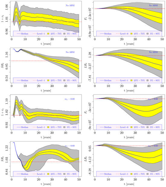
Figure 7.
Simulated dynamics of , , , and (50-year-long projection horizon). The pension system adopted the Italian setting (i.e., historical data were considered up to 2024) and obeyed Equations (10) and (15). For the top panels (first and second rows), no ABM was applied. For the bottom panels (third and fourth rows), a symmetric mixed ABM () was applied.
4.3.2. Sensitivities over a 50-Year Projection Horizon
As discussed above in Section 4.1.1, the estimated value in the “2024 Italian” setting can be regarded as a stressed value heavily driven by the very last years in the time series. Indeed, it cannot be interpreted as a long-term average, since unmodeled factors such as migration and political actions would force it to increase in the long run. In the following, we consider a stressed value for the other three trend parameters , , and , which drive the inflation rate, salary growth rate, and employment rate, respectively. The same mixed ABM discussed in Section 4.3.1 was applied to assess the robustness of the ABM behavior as the parameters of each risk factor were varied. Since we considered the “2024 Italian” a stressed value itself, the three stresses discussed below consider the “2015 Italian” while maintaining the rest of the parameters as estimated under the “2024 Italian” setting. The parameter values calibrated in the two settings are available in Appendix A. The three stressed parameterizations are as follows. For the first one, the inflation rate trend was doubled with respect to the “2024 Italian” calibrated value. For the second, the employment rate trend was fixed to a negative value (). Finally, for the third one, the salary growth rate trend was nullified. Hence, when also considering the simulation presented in Section 4.3.1 above, all four risk factors were involved in the sensitivity analysis. The outputs of the three stressed parameterizations are shown in Appendix D. The results obtained demonstrate the robustness of the model and the mixed ABM behavior as they are hardly distinguishable from each other, and the effects of the mixed ABM on the considered system variables were almost identical to those already displayed and commented on in Section 4.3.1.
5. Summary
This work proposed and assessed a novel “mixed” ABM that combines balance mechanisms based on the liquidity ratio (LR) and solvency ratio (SR) through a weight , coupled with a dampening mechanism that imposes smoothness constraints on adjustments to the notional rate and indexation. The analysis was conducted in a realistic stochastic environment (calibrated on Italian data) in which demographic and economic processes—driving contribution inflows and pension outflows—co-evolve. The performance of the ABMs was evaluated by considering a multi-objective criterion. Indeed, we assessed both the stability of the notional rate (minimizing the maximum volatility ) and its adequacy (maximizing the minimum Sharpe ratio ). Furthermore, financial sustainability was also considered by controlling the risk of the buffer fund through a value-at-risk-like criterion inspired by the Basel and Solvency regulatory frameworks.
Simulations showed that across a broad subset of configurations (symmetric or asymmetric; multiple horizons, dynamic, or fixed retirement age, with and without survivor dividend), solutions existed for the weight that jointly improved the stability of and the risk profile of the buffer fund relative to the “pure” rules (LR-only or SR-only). Therefore, compared with single-indicator ABMs, the mixed formulation exhibited stronger risk mitigation properties. In the Italian setting, under a symmetric ABM, a mixed ABM with emerged as the solution that simultaneously optimized social utility and financial sustainability. Under an asymmetric ABM, the mixed rule acts as a suboptimal yet robust compromise, reconciling objectives that are often in tension (short-term cash stability versus medium-to-long-term balance sheet position) without uniformly dominating the alternatives in every scenario. In terms of adequacy, a mixed ABM mitigated the volatility extremes induced by LR while preserving much of SR’s advantage in terms of reward to variability, as highlighted in the literature. With dampening, the mixed rule limited tail risk for , avoiding both persistent liquidity imbalances and excessive asset accumulation (inefficiency), in line with the proposed VaR-like criterion for .
It is also informative to compare these results with [12], which showed that within a four-cohort OLG model with the NDC Swedish approach, an SR-based ABM reduced the volatility of the buffer fund and delivered, in most cases, a Sharpe ratio higher than that of the alternative LR-based rule. However, SR may fail to restore liquidity in all circumstances. Relative to that evidence, the present work generalized the “SR or LR” dichotomy by introducing a continuous mix with smoothness constraints and a multi-criteria framework (Sharpe ratio or volatility of plus risk control for ) on an age-structured demographic model calibrated for Italy. The results indicate that a mixed combination can replicate much of SR’s advantage in terms of reward to variability while compensating for SR’s short-run limitations in liquidity, and it reduces operational swings through dampening.
5.1. Model Limitations and Future Extensions
The proposed stochastic actuarial framework is designed to be parsimonious and transparent, following conventions widely adopted in actuarial analyses of PAYG-NDC systems. Nevertheless, several simplifying assumptions restrict its interpretative scope and identify potential directions for further extensions. Firstly, the model assumes a closed demographic system, excluding migration flows. This assumption is consistent with the standard actuarial literature on PAYG-NDC balance sheet modeling, where population dynamics are typically represented through fertility and mortality only [6,12,14]. Such an approach enables an internally coherent analysis of financial sustainability and intergenerational consistency, independent of external demographic adjustments. However, in the Italian context, where net migration has significantly contributed to labor force growth since the 1990s [34], this assumption likely overstates the projected decline in the contributor base and the speed of population aging. Future developments could incorporate migration as a stochastic or policy-driven process to capture its potential mitigating role for demographic imbalances. Fertility and productivity growth are modeled as exogenous processes with constant drift and volatility parameters. This simplification enables tractable stochastic simulations but omits structural or policy-induced changes. Empirical evidence suggests that fertility rates in low-fertility European countries may respond, at least partially, to family and labor market policies [35], while productivity trends can shift with technological change and labor market dynamics [23]. Introducing mean-reverting or regime-switching dynamics could better represent such long-term transitions. The simulations assume policy continuity without exogenous reforms to the contribution rates, retirement ages, or indexation rules. In practice, real-world pension systems are subject to institutional adjustments that may interact with automatic balancing mechanisms. Future applications could integrate adaptive or scenario-based policy interventions. The model indirectly captured the short-term demographic and macroeconomic consequences of the COVID-19 pandemic through the calibration up to 2024, but no explicit shock process was included. Although excess mortality and temporary fertility reductions have been observed in Italy and other OECD countries during 2020–2021 [23,34], their long-term effects on pension system dynamics appear to be limited. Nonetheless, extending the stochastic structure to accommodate rare event shocks, such as pandemics or financial crises, would enhance the robustness of long-term risk assessments.
5.2. Further Developments of This Work
The proposed framework opens up further developments under different perspectives.
First, it is worth investigating whether and under which conditions the most generalized mixed ABM introduced in Section 3.2 may bring further benefits to an NDC pension system. This version of the problem would require a significant effort in terms of further numerical research, as the dimensionality of the parameter space would increase from one to three, while still considering multiple independent objective functions. Furthermore, the mixed ABM weights are assumed to be independent of time and macroeconomic context; however, part of the numerical results reported in Section 4.2.2 suggest that the optimal ABM parameterization may change over time. Thus, it would be possible to generalize the framework further by introducing weight dynamics. This extension implies the need to identify optimal weight trajectories instead of optimal values. The complexity of the resulting problem could be handled through machine learning techniques, such as neural networks.
Moreover, structural stress testing could be extended through the a priori introduction of complex scenarios (e.g., unanticipated longevity shocks or multiple baby booms or busts) to compare LR-based, SR-based, and mixed ABMs, aiming to measure the resilience of the different rules when demographic and economic shocks interact and propagate over time.
It may also be worthwhile to broaden adequacy metrics beyond the Sharpe ratio by including downside risk measures with , such as semi-variance and expected shortfall. From a social perspective, these indicators are also worth being investigated, as they asymmetrically penalize adverse outcomes and help calibrate dampening and triggers to limit the regressive effects of unfavorable episodes.
This research could also be extended by making individual-level heterogeneity explicit: distributions of pensions by cohort and gender, the sensitivity of contribution careers, and measures of intergenerational risk sharing. Within this framework, actuarial fairness should be assessed as a dynamic property, verifying the consistency of the intergenerational transfers induced by the ABM over multi-year horizons.
From a policy perspective, the practical implementation of a mixed ABM would require clear governance and communication tools. While the mechanism introduces analytical complexity, its operational form could remain transparent if based on observable quantities (liquidity and solvency ratios) published within the pension system’s annual actuarial balance sheet. The adjustment weights could be fixed or periodically reviewed by an independent body and disclosed through standardized reporting instruments, similar to the Swedish Orange Report. This would ensure both comprehensibility for stakeholders and legitimacy of automatic corrections, aligning the mixed rule with the communication standards already established for existing ABMs. Future developments could explicitly integrate this governance dimension. The definition of triggers (liquidity and solvency thresholds) should be aligned with actuarial accounting practices and with transparent reporting tools such as the Orange Report, thereby strengthening accountability and facilitating communication of the rules to decision makers and the public.
Author Contributions
Conceptualization, J.G.; methodology, J.G. and M.M.; software, J.G. and M.M.; validation, J.G. and M.M.; formal analysis, J.G. and M.M.; investigation, J.G. and M.M.; resources, J.G. and M.M.; data curation, J.G. and M.M.; writing—original draft, J.G. and M.M.; writing—review and editing, J.G. and M.M.; supervision, M.M. All authors have read and agreed to the published version of the manuscript.
Funding
This research received no external funding.
Data Availability Statement
The data that support the findings of this study are openly available from “IstatData—The Italian National Institute of Statistics data warehouse” [32] and the “Human Mortality Database” [33].
Conflicts of Interest
The authors declare that the research was conducted in the absence of any commercial or financial relationships that could be construed as a potential conflict of interest.
Appendix A. Details on Calibration and Data Sources
This section provides further information on the input datasets and calibration outputs. The parameterization of each considered configuration of the model is displayed in Table A1, Table A2, Table A3, Table A4, Table A5, Table A6 and Table A7. The time series utilized in calibrating the model are listed in Table A8.

Table A1.
Parameterization of the risk factors considered in each setting.
Table A1.
Parameterization of the risk factors considered in each setting.
| Risk Factor | 2015-ITA | 2024-ITA | Driftless | ||||
|---|---|---|---|---|---|---|---|
| Inflation | 0.0161 | 0.0099 | 0.0191 | 0.0167 | 0.0000 | 0.0099 | |
| Salaries | g | 0.0194 | 0.0103 | 0.0198 | 0.0193 | 0.0000 | 0.0103 |
| Natality | n | −0.0013 | 0.0070 | −0.0051 | 0.0109 | 0.0000 | 0.0070 |
| Employment | o | 0.0093 | 0.0262 | 0.0131 | 0.0369 | 0.0000 | 0.0262 |
Table A2.
Correlation matrix among the risk factors considered in each setting.
Table A2.
Correlation matrix among the risk factors considered in each setting.
| 2015-ITA; Driftless | ||||
| z | g | n | o | |
| 1.000 | 0.505 | 0.494 | 0.051 | |
| g | 0.505 | 1.000 | 0.650 | −0.121 |
| n | 0.494 | 0.650 | 1.000 | −0.605 |
| o | 0.051 | −0.121 | −0.605 | 1.000 |
| 2024-ITA | ||||
| z | g | n | o | |
| 1.000 | 0.349 | 0.057 | 0.420 | |
| g | 0.349 | 1.000 | 0.123 | 0.045 |
| n | 0.057 | 0.123 | 1.000 | −0.033 |
| o | 0.420 | 0.045 | −0.033 | 1.000 |
Table A3.
Lee–Carter model calibration: parameters of per gender and setting.
Table A3.
Lee–Carter model calibration: parameters of per gender and setting.
| Process | 2015-ITA; Driftless | 2024-ITA | ||||||
|---|---|---|---|---|---|---|---|---|
| Females (i = 1) | Males (i = 2) | Females (i =1) | Males (i = 2) | |||||
| −1.594 | 2.153 | −1.526 | 1.491 | −1.584 | 2.145 | −1.512 | 1.480 | |
Table A4.
Lee–Carter model calibration, with death probabilities (i.e., ; ) introduced in Equation (30) and calibrated through Italian historical data up to 2015. The parameter associated with the xth cohort is displayed in the cell , where .
Table A4.
Lee–Carter model calibration, with death probabilities (i.e., ; ) introduced in Equation (30) and calibrated through Italian historical data up to 2015. The parameter associated with the xth cohort is displayed in the cell , where .
| 0.0002 | 0.0002 | 0.0002 | 0.0002 | 0.0002 | 0.0002 | 0.0002 | 0.0002 |
| 0.0002 | 0.0003 | 0.0003 | 0.0003 | 0.0003 | 0.0003 | 0.0003 | 0.0004 |
| 0.0004 | 0.0004 | 0.0005 | 0.0005 | 0.0006 | 0.0006 | 0.0007 | 0.0008 |
| 0.0009 | 0.0010 | 0.0011 | 0.0011 | 0.0012 | 0.0014 | 0.0015 | 0.0017 |
| 0.0019 | 0.0020 | 0.0022 | 0.0023 | 0.0025 | 0.0028 | 0.0030 | 0.0033 |
| 0.0035 | 0.0039 | 0.0042 | 0.0046 | 0.0051 | 0.0057 | 0.0062 | 0.0068 |
| 0.0075 | 0.0082 | 0.0091 | 0.0102 | 0.0114 | 0.0128 | 0.0145 | 0.0164 |
| 0.0185 | 0.0212 | 0.0241 | 0.0276 | 0.0318 | 0.0367 | 0.0424 | 0.0489 |
| 0.0559 | 0.0645 | 0.0743 | 0.0853 | 0.0971 | 0.1103 | 0.1249 | 0.1417 |
| 0.1581 | 0.1753 | 0.1948 | 0.2143 | 0.2366 | 0.2580 | 0.2793 | 0.2983 |
Table A5.
Lee–Carter model calibration, with death probabilities (i.e., ; ) introduced in Equation (30) and calibrated through Italian historical data up to 2015. The parameter associated with the xth cohort is displayed in the cell , where .
Table A5.
Lee–Carter model calibration, with death probabilities (i.e., ; ) introduced in Equation (30) and calibrated through Italian historical data up to 2015. The parameter associated with the xth cohort is displayed in the cell , where .
| 0.0005 | 0.0006 | 0.0006 | 0.0006 | 0.0006 | 0.0007 | 0.0007 | 0.0007 |
| 0.0007 | 0.0007 | 0.0007 | 0.0007 | 0.0007 | 0.0008 | 0.0008 | 0.0008 |
| 0.0008 | 0.0008 | 0.0009 | 0.0009 | 0.0010 | 0.0011 | 0.0011 | 0.0012 |
| 0.0013 | 0.0014 | 0.0016 | 0.0017 | 0.0019 | 0.0021 | 0.0023 | 0.0025 |
| 0.0028 | 0.0031 | 0.0035 | 0.0039 | 0.0042 | 0.0047 | 0.0053 | 0.0058 |
| 0.0065 | 0.0072 | 0.0079 | 0.0088 | 0.0096 | 0.0107 | 0.0119 | 0.0131 |
| 0.0143 | 0.0159 | 0.0175 | 0.0194 | 0.0214 | 0.0239 | 0.0266 | 0.0297 |
| 0.0333 | 0.0370 | 0.0417 | 0.0472 | 0.0533 | 0.0596 | 0.0675 | 0.0763 |
| 0.0859 | 0.0962 | 0.1084 | 0.1205 | 0.1357 | 0.1506 | 0.1659 | 0.1838 |
| 0.2018 | 0.2205 | 0.2406 | 0.2615 | 0.2836 | 0.3088 | 0.3288 | 0.3461 |
Table A6.
Lee–Carter model calibration, with death probabilities (i.e., ; ) introduced in Equation (30) and calibrated through Italian historical data up to 2024. The parameter associated with the xth cohort is displayed in the cell , where .
Table A6.
Lee–Carter model calibration, with death probabilities (i.e., ; ) introduced in Equation (30) and calibrated through Italian historical data up to 2024. The parameter associated with the xth cohort is displayed in the cell , where .
| 0.0002 | 0.0002 | 0.0002 | 0.0002 | 0.0002 | 0.0002 | 0.0002 | 0.0002 |
| 0.0002 | 0.0003 | 0.0003 | 0.0003 | 0.0003 | 0.0003 | 0.0003 | 0.0004 |
| 0.0004 | 0.0004 | 0.0005 | 0.0005 | 0.0006 | 0.0006 | 0.0007 | 0.0008 |
| 0.0009 | 0.0010 | 0.0011 | 0.0011 | 0.0013 | 0.0014 | 0.0015 | 0.0017 |
| 0.0019 | 0.0020 | 0.0022 | 0.0023 | 0.0025 | 0.0028 | 0.0030 | 0.0033 |
| 0.0036 | 0.0040 | 0.0043 | 0.0047 | 0.0052 | 0.0057 | 0.0062 | 0.0069 |
| 0.0075 | 0.0083 | 0.0092 | 0.0102 | 0.0114 | 0.0128 | 0.0145 | 0.0165 |
| 0.0186 | 0.0213 | 0.0242 | 0.0277 | 0.0320 | 0.0369 | 0.0426 | 0.0492 |
| 0.0561 | 0.0647 | 0.0745 | 0.0857 | 0.0975 | 0.1108 | 0.1255 | 0.1424 |
| 0.1590 | 0.1764 | 0.1961 | 0.2156 | 0.2377 | 0.2589 | 0.2803 | 0.2987 |
Table A7.
Lee–Carter model calibration, with death probabilities (i.e., ; ) introduced in Equation (30) and calibrated through Italian historical data up to 2024. The parameter associated with the xth cohort is displayed in the cell , where .
Table A7.
Lee–Carter model calibration, with death probabilities (i.e., ; ) introduced in Equation (30) and calibrated through Italian historical data up to 2024. The parameter associated with the xth cohort is displayed in the cell , where .
| 0.0005 | 0.0006 | 0.0006 | 0.0006 | 0.0006 | 0.0007 | 0.0007 | 0.0007 |
| 0.0007 | 0.0007 | 0.0007 | 0.0007 | 0.0007 | 0.0008 | 0.0008 | 0.0008 |
| 0.0008 | 0.0008 | 0.0009 | 0.0009 | 0.0010 | 0.0011 | 0.0011 | 0.0013 |
| 0.0013 | 0.0015 | 0.0016 | 0.0017 | 0.0019 | 0.0021 | 0.0023 | 0.0025 |
| 0.0028 | 0.0031 | 0.0035 | 0.0039 | 0.0042 | 0.0047 | 0.0053 | 0.0058 |
| 0.0065 | 0.0072 | 0.0080 | 0.0088 | 0.0097 | 0.0107 | 0.0119 | 0.0131 |
| 0.0144 | 0.0159 | 0.0175 | 0.0195 | 0.0215 | 0.0240 | 0.0267 | 0.0298 |
| 0.0334 | 0.0371 | 0.0417 | 0.0473 | 0.0540 | 0.0605 | 0.0685 | 0.0770 |
| 0.0865 | 0.0967 | 0.1091 | 0.1214 | 0.1366 | 0.1516 | 0.1672 | 0.1853 |
| 0.2036 | 0.2224 | 0.2425 | 0.2639 | 0.2865 | 0.3125 | 0.3333 | 0.3508 |
Table A8.
Time series utilized in this work. The same datasets have been elaborated across all the settings by truncating the data at two different reference dates. The available observation ranges refer to access made on 31 March 2025.
Table A8.
Time series utilized in this work. The same datasets have been elaborated across all the settings by truncating the data at two different reference dates. The available observation ranges refer to access made on 31 March 2025.
| Risk Factor | Time Series Name | Range | Database |
|---|---|---|---|
| Inflation | Indices of consumer prices for blue and white collar worker households | 1861–2015 | https://seriestoriche.istat.it/ |
| Consumer price index for blue and white collar worker households (base 2015 = 100): annual average | 2016–2024 | https://esploradati.istat.it/databrowser/ | |
| Salaries | Annual contractual gross wages of some professional categories for some economy sectors | 1990–2015 | https://seriestoriche.istat.it/ |
| Compensation of employees and its components by industry | 2015–2024 | https://esploradati.istat.it/databrowser/ | |
| Natality | Resident population age 15 and over by professional status, age group, and geographical area | 1977–2015 | https://seriestoriche.istat.it/ |
| Demographic indicators | 2002–2024 | https://esploradati.istat.it/databrowser/ | |
| Employment | Employment rates, unemployment rates, and activity rates by age group, sex, region, and geographical area | 1977–2015 | https://seriestoriche.istat.it/ |
| Employed persons: statistical back recalculation since 2004 (age) | 2004–2024 | https://esploradati.istat.it/databrowser/ | |
| Mortality (females) | Life tables: females | 1872–2022 | https://www.mortality.org/ |
| Mortality (males) | Life tables: males | 1872–2022 | https://www.mortality.org/ |
Comparison with Official RGS Projections
Although producing projections of pension expenditure comparable with those by the Ragioneria Generale dello Stato (RGS) or the OECD is beyond the scope of this study, we report below some summary indicators of the demographic and economic evolution of the pension system (adopting the 2024 Italian setting) for illustrative comparison with the official RGS projections [36].
These values are not directly comparable, as our framework adopts simplifying assumptions consistent with the methodological objective of testing ABMs rather than replicating the Italian pension system. The main differences are as follows. Our model is unisex; wage and pension parameters refer to private sector employees only (over 50% of total expenditure), whereas RGS projections cover all schemes; demographic dynamics are simplified for fertility and employment and exclude migration; the notional rate is indexed to wage bill growth (consistent with the canonical NDC approach) instead of to nominal GDP growth, as in the RGS model (in accordance with current Italian legislation); and minimum and maximum benefit constraints are not applied.
Despite these differences, the reported results indicate that the simulated values remained within a plausible range and that observed discrepancies stemmed from modeling assumptions that did not affect the robustness of the ABM comparative analysis.
Table A9.
Comparison between RGS 2025 and our simulations.
Table A9.
Comparison between RGS 2025 and our simulations.
| Pensioner-to- Employed Ratio (%) | Gross Replacement Rate (%) | |||||
|---|---|---|---|---|---|---|
| Years | 2024 | 2048 | 2070 | 2030 | 2050 | 2070 |
| RGS 2025 | 60.4% | 76.8% | 72.7% | 72.1% | 60.3% | 58.4% |
| Median our model | 67.1% | 80.8% | 102.8% | 61.4% | 61.6% | 48.5% |
In particular, we observed that in our setting, the initial value of the pensioner-to-employed ratio was higher than in the RGS projection (67% vs. 60%), although both indicators increased markedly over the first 24 years and tended to converge (81% vs. 77%). The divergence over the longer horizon is explained by the specific assumptions of the “Italy 2024” setting, characterized by a strongly negative process drift not compensated by migration flows (see the discussion in Section 4).
The difference in the gross replacement rate in 2030 (61% vs. 72%) can be attributed to the fact that in our model—as explained in Section 4—pension expenditure is normalized to represent a system already operating under a fully implemented NDC scheme, whereas the RGS values reflect that newly awarded pensions are determined under a mixed DB-NDC scheme, with a highly generous DB component. The two values become closer by 2050 (62% vs. 60%), when both systems have reached full NDC maturity. The wider gap in 2070 (49% vs. 58%) is mainly due to the fact that in our framework, the notional capital was revalued according to wage bill growth—which in our setting was affected by the decline in the active population discussed above—and the absence of minimum benefit provisions in our model.
Appendix B. Additional Material on the “2015 Italian” Case Study
With specific reference to the configuration described in Section 4.2.1, the solutions to the problems from Equations (48)–(55) are displayed below for all three simulated time horizons.

Figure A1.
Numerical solutions to the problems stated in Equations (48) (left panels) and (49) (right panels) for the pensions system represented in Figure 3 above. From the top to the bottom rows, different values are considered: 150, 100, and 50, respectively. The optimal value is marked by the purple dashed line. The pink neighborhood around each optimal value displays the suboptimal solutions within a 15% tolerance.

Figure A2.
Numerical solutions to the problems stated in Equations (54) (left panels) and (55) (right panels) for the pension system represented in Figure 3 above. From the top to the bottom rows, different values are considered: 150, 100, and 50, respectively. Color conventions are the same as those utilized in Figure A1 above.
Appendix C. Additional Material on the “2024 Italian” Case Study
With specific reference to the configuration described in Section 4.3.1, the solutions to the problems from Equations (48)–(55) are displayed below for two simulated time horizons.

Figure A3.
Numerical solutions to the problems stated in Equations from (48) to (55) for the pension system analyzed in Section 4.3.1 above. From the top to the bottom rows, different values are considered: 50 (first and third rows) and 25 (second and fourth rows). Color conventions are the same as those utilized in Figure A1 above.
Appendix D. Sensitivities for the “2024 Italian” Case Study
This appendix reports the outputs of the simulations described in Section 4.3.2.

Figure A4.
Simulated dynamics of , , , and (50-year-long projection horizon). The specifics are the same as those considered in Figure 7, except for , as calibrated in the “2015 Italian” setting, and , which is twice the value calibrated in the “2024 Italian” setting.

Figure A5.
Simulated dynamics of , , , and (50-year-long projection horizon). The specifics are the same as those considered in Figure 7, except for , as calibrated in the “2015 Italian” setting, and , which is set to .

Figure A6.
Simulated dynamics of , , , and (50-year-long projection horizon). The specifics are the same as those considered in Figure 7, except for , as calibrated in the “2015 Italian” setting, and , which is set to zero.
References
- Palmer, E. What’s NDC? In Pension Reform; Holzmann, R., Palmer, E., Eds.; World Bank: Washington, DC, USA, 2006; Chapter 2; pp. 17–35. [Google Scholar]
- Chłón-Domińczak, A.; Franco, D.; Palmer, E. The first wave of NDC reforms. In NDC Pension Schemes in a Changing Pension World; Holzmann, R., Palmer, P., Robalino, D., Eds.; World Bank: Washington, DC, USA, 2012; Volume 1, pp. 31–85. [Google Scholar]
- Holzmann, R. The ABCs of nonfinancial defined contribution (NDC) schemes. Int. Soc. Secur. Rev. 2017, 70, 53–77. [Google Scholar] [CrossRef]
- Alonso-García, J.; Boado-Penas, M.; Devolder, P. Adequacy, fairness and sustainability of pay-as-you-go pension systems: Defined benefit versus defined contribution. Eur. J. Financ. 2018, 24, 1100–1122. [Google Scholar] [CrossRef]
- Settergren, O.; Mikula, B.D. The rate of return of pay-as-you-go pension systems: A more exact consumption-loan model of interest. J. Pension Econ. Financ. 2005, 4, 115–138. [Google Scholar] [CrossRef]
- Godínez-Olivares, H.; Boado-Penas, M.; Haberman, S. Optimal strategies for pay-as-you-go pension finance: A sustainability framework. Insur. Math. Econ. 2016, 69, 117–126. [Google Scholar] [CrossRef]
- Gronchi, S.; Nisticò, S. Implementing the NDC theoretical model: A comparison of Italy and Sweden. In Pension Reform: Issues and Prospect for Non-Financial Defined Contribution (NDC) Schemes; Holzmann, R., Palmer, G., Eds.; World Bank: Washington, DC, USA, 2006; Chapter 19; pp. 493–515. [Google Scholar]
- Valdés-Prieto, S. The financial stability of notional account pensions. Scand. J. Econ. 2000, 102, 395–417. [Google Scholar] [CrossRef]
- Vidal-Meliá, C.; Boado-Penas, M.; Settergren, O. Automatic balance mechanisms in PAYG pension systems. Geneva Pap. Risk Insur. Issues Pract. 2009, 34, 287–317. [Google Scholar] [CrossRef]
- Knell, M. How automatic adjustment factors affect the internal rate of return of PAYG pension systems. J. Pension Econ. Financ. 2010, 9, 1–23. [Google Scholar] [CrossRef]
- Settergren, O. The automatic balance mechanism of the Swedish pension system—A non-technical introduction. Wirtsch. Bl. 2001, 4, 339–349. [Google Scholar]
- Alonso-García, J.; Boado-Penas, M.; Devolder, P. Automatic balancing mechanisms for notional defined contribution accounts in the presence of uncertainty. Scand. Actuar. J. 2018, 2, 85–108. [Google Scholar] [CrossRef]
- Alonso-García, J.; Devolder, P. Continuous time model for notional defined contribution pension schemes: Liquidity and solvency. Insur. Math. Econ. 2019, 88, 57–76. [Google Scholar] [CrossRef]
- Devolder, P.; Levantesi, S.; Menzietti, M. Automatic balance mechanisms for notional defined contribution pension systems guaranteeing social adequacy and financial sustainability: An application to the Italian pension system. Ann. Oper. Res. 2021, 299, 765–795. [Google Scholar] [CrossRef]
- Zaidi, A.; Rake, K. Dynamic Microsimulation Models: A Review and Some Lessons for SAGE; Department of Work and Pensions Research Report, 153; London School of Economics: London, UK, 2001. [Google Scholar]
- Dekkers, G.; Buslei, H.; Cozzolino, M.; Desmet, R.; Geyer, J.; Hofmann, D.; Raitano, M.; Steiner, V.; Tanda, P.; Tedeschi, S.; et al. What Are the Consequences of the AWG-Projections for the Adequacy of Social Security Pensions? ENEPRI Research Report No. 65; Centre for European Policy Studies: Brussels, Belgium, 2009; ISBN 978-92-9079-846-0. Available online: https://www.ceps.eu/ceps-publications/what-are-consequences-awg-projections-adequacy-social-security-pensions/ (accessed on 20 September 2025).
- Li, J.; O’Donoghue, C. A survey of dynamic microsimulation models: Uses, model structure and methodology. Int. J. Microsimul. 2013, 6, 3–55. [Google Scholar] [CrossRef]
- Auerbach, A.J.; Kotlikoff, L. Dynamic Fiscal Policy; Cambridge University Press: Cambridge, UK, 1987; ISBN 9780521311127. [Google Scholar]
- Fehr, H.; Kallweit, M.; Kindermann, F. Pension reform with variable retirement age: A simulation analysis for Germany. J. Pension Econ. Financ. 2012, 11, 389–417. [Google Scholar] [CrossRef]
- Heer, B.; Irmen, A. Population, pensions, and endogenous economic growth. J. Econ. Dyn. Control 2014, 46, 50–72. [Google Scholar] [CrossRef]
- Börsch-Supan, A.; Ludwig, A.; Winter, J. Ageing, Pension Reform, and Capital Flows: A Multi-Country Simulation Model. Economica 2006, 73, 625–658. [Google Scholar] [CrossRef]
- Holzmann, R.; Palmer, E. Pension Reform: Issues and Prospects for Non-Financial Defined Contribution (NDC) Schemes; World Bank: Washington, DC, USA, 2006; ISBN 9780821365777. [Google Scholar]
- OECD. Pensions at a Glance 2023: OECD and G20 Indicators; OECD Publishing: Paris, France, 2023. [Google Scholar] [CrossRef]
- Boado-Penas, M.; Vidal-Melìa, C. Nonfinancial defined contribution pension schemes: Is a survivor dividend necessary to make the system balanced? Appl. Econ. Lett. 2014, 21, 242–247. [Google Scholar] [CrossRef]
- Lee, R.D.; Carter, L.R. Modeling and Forecasting U. S. Mortality. J. Am. Stat. Assoc. 1992, 87, 659–671. [Google Scholar] [CrossRef] [PubMed]
- Alho, J.; Bravo, J.; Palmer, E. Annuities and life expectancy in ndc. In Nonfinancial Defined Contribution Pension Schemes in a Changing PensionWorld—Volume 2: Gender, Politics, and Financial Stability; Holzmann, R., Palmer, E., Robalino, D., Eds.; The World Bank: Washington, DC, USA, 2013; Chapter 22; pp. 395–443. ISBN 978-0-8213-8852-5. [Google Scholar]
- Palmer, E. Generic ndc: Equilibrium, valuation, and risk sharing with and without ndc bonds. In Nonfinancial Defined Contribution Pension Schemes in a Changing Pension World—Volume 2: Gender, Politics, and Financial Stability; Holzmann, R., Palmer, E., Robalino, D., Eds.; The World Bank: Washington, DC, USA, 2013; Chapter 10; pp. 309–343. ISBN 978-0-8213-8852-5. [Google Scholar]
- Franco, D. Italy: A never-ending pension reform. In Social Security Pension Reform in Europe; Feldstein, M., Siebert, H., Eds.; University of Chicago Press: Chicago, IL, USA, 2002; pp. 202–245. [Google Scholar]
- Borella, M.; Coda Moscarola, F. The 2011 Pension Reform in Italy and Its Effects on Current and Future Retirees; CeRP Working Papers 151; Center for Research on Pensions and Welfare Policies: Turin, Italy, 2015. [Google Scholar]
- Bevilacqua, G.; Nisticò, S.; Gronchi, S. The Italian NDC Scheme: Evolution and Remaining Potholes. In Progress and Challenges of Nonfinancial Defined Contribution Pension Schemes—Volume 1: Addressing Marginalization, Polarization, and the Labor Market; Holzmann, R., Palmer, E., Palacios, R., Sacchi, S., Eds.; The World Bank: Washington, DC, USA, 2020; Chapter 4; pp. 73–90. ISBN 978-1-4648-1453-2. [Google Scholar]
- Mazzaferro, C. The transition to NDC in Italy: Assessing distributive and financial effects. J. Pension Econ. Financ. 2023, 22, 116–131. [Google Scholar] [CrossRef]
- IstatData—The Italian National Institute of Statistics Data Warehouse. Available online: https://esploradati.istat.it/databrowser/#/it/dw/categories (accessed on 20 July 2025).
- Human Mortality Database. Available online: https://www.mortality.org/ (accessed on 25 July 2025).
- ISTAT. Demographic Indicators and Migration Statistics. 2023. Available online: https://www.istat.it/en/population-and-households (accessed on 1 October 2025).
- Matysiak, A.; Sobotka, T.; Vignoli, D. The Great Recession and Fertility in Europe: A Sub-national Analysis. Eur. J. Popul. 2021, 37, 29–64. [Google Scholar] [CrossRef] [PubMed]
- Ragioneria Generale dello Stato. Le Tendenze di Medio-Lungo Periodo del Sistema Pensionistico e Socio-Sanitario; Rapporto n. 26; Giugno 2025. Available online: https://www.rgs.mef.gov.it/VERSIONE-I/attivita_istituzionali/monitoraggio/spesa_pensionistica/ (accessed on 20 September 2025).
Disclaimer/Publisher’s Note: The statements, opinions and data contained in all publications are solely those of the individual author(s) and contributor(s) and not of MDPI and/or the editor(s). MDPI and/or the editor(s) disclaim responsibility for any injury to people or property resulting from any ideas, methods, instructions or products referred to in the content. |
© 2025 by the authors. Licensee MDPI, Basel, Switzerland. This article is an open access article distributed under the terms and conditions of the Creative Commons Attribution (CC BY) license (https://creativecommons.org/licenses/by/4.0/).