Abstract
This paper develops and analyzes new high-order iterative schemes for the effective evaluation of the matrix square root (MSR). By leveraging connections between the matrix sign function and the MSR, we design stable algorithms that exhibit fourth-order convergence under mild spectral conditions. Detailed error bounds and convergence analyses are provided, ensuring both theoretical rigor and numerical reliability. A comprehensive set of numerical experiments, conducted across structured and large-scale test matrices, demonstrates the superior performance of the proposed methods compared to classical approaches, both in terms of computational efficiency and accuracy. The results confirm that the proposed iterative strategies provide robust and scalable tools for practical applications requiring repeated computation of matrix square roots.
Keywords:
matrix square root; iterative methods; convergence analysis; computational efficiency; Jordan canonical form MSC:
65F60; 41A25
1. Introductory Notes
The study of matrix functions occupies a central role in modern computational mathematics and its applications across diverse scientific domains. A matrix function is defined as a rule that assigns to a square matrix another matrix of the same dimension, based on some functional relation that extends scalar functions to the matrix setting. Classical definitions rely on the Jordan canonical form, the integral of Cauchy representation, or Hermite matrix polynomial expansions, each of which provides an equivalent but distinct perspective on how functions act on matrices [1]. These formulations are not merely of theoretical interest; rather, they constitute the essential building blocks for developing computational algorithms that can handle large-scale problems in engineering and data science.
Traditional techniques such as diagonalization or contour integration have long been used to evaluate matrix functions. However, their practical implementation is often limited by the need for spectral decompositions or by sensitivity to conditioning when dealing with non-normal or nearly defective matrices. In contrast, iterative schemes have gained increasing prominence [2], especially in large-scale or real-time applications where data evolves dynamically or when good-quality initial approximations are available [3,4]. Iterative methods improve computational tractability while offering flexible trade-offs between accuracy and efficiency.
The matrix square root (MSR) X of a provided matrix A is defined such that
In practical numerical applications, one may encounter the need to compute both X and its inverse simultaneously [5]. This coupled problem can be reformulated as finding a solution X that minimizes the residual
with the corresponding cost function given by
The MSR of A, shown by , is any matrix X such that . Unless otherwise specified, refers to the principal square root. Note that denotes the inverse of the principal square root, i.e., ; see also [6]. In this formulation, the goal is to drive the residual to zero. Similarly to the nonlinear least-squares problem discussed earlier, a natural approach is to adopt a Newton-type iteration. However, matrices that are ill-conditioned or which exhibit clustered eigenvalues may impair the performance of the classical Newton or even Gauss–Newton iterations, thus necessitating higher-order corrections.
The present work focuses on the iterative computation of the MSR and its inverse. This problem is of considerable importance both theoretically and practically. For example, in the resolution of nonlinear and linear matrix differential equations, MSRs naturally arise in closed-form solutions. Consider the first-order system
where A is a matrix with a well-defined square root and is a prescribed source term. The solution can be expressed explicitly as
Here, the exponential of the MSR governs the dynamical evolution. Similarly, in second-order matrix differential Equations [1] of oscillatory type,
the exact solution is given by
whereas both the principal square root and its inverse play crucial roles. The MSR is tightly linked to a family of related matrix functions, such as the matrix exponential, logarithm, cosine, and sine. These interconnections provide both theoretical insight and computational pathways [7].
1.1. Exponential and Logarithm
For a nonsingular matrix A with no eigenvalues on the closed negative real axis, one can define [8]
wherein is the principal matrix logarithm. This relation emphasizes that efficient algorithms for the matrix logarithm can indirectly yield algorithms for the square root.
1.2. Trigonometric Functions
In oscillatory systems, one often encounters
Here, the inverse square root plays an indispensable role in the evaluation of the sine function, as in the resolution of second-order differential equations.
1.3. The Sign of a Matrix
The connection between the MSR and the sign function is fundamental. For a nonsingular A,
which shows that an efficient algorithm for the sign function can be adapted to calculate the square root, and vice versa.
1.4. Control Theory
In linear quadratic regulator (LQR) problems, the Riccati (algebraic) equation
is central. Numerical solvers frequently exploit the Hamiltonian matrix
whose stable invariant subspace is determined via the matrix sign function. Since computation depends on MSR algorithms, iterative schemes for the square root are vital in control applications [9].
1.5. Quantum Mechanics
The time evolution of a quantum system is controlled by the Schrödinger equation
with Hamiltonian H. When considering reduced models, one often computes
for propagator approximations. Hence, square root operators are crucial for both exact and approximate quantum dynamics.
1.6. Data Science and Machine Learning
In covariance estimation, whitening transformations, and kernel methods, the MSR is indispensable. Given a positive semidefinite covariance matrix ,
produces whitened data with identity covariance. Efficient computation of is therefore a fundamental preprocessing step in statistical learning. See also Table 1.

Table 1.
Applications of the MSR and its inverse across disciplines.
Direct methods for computing MSRs—such as Schur decomposition followed by block square rooting—are numerically reliable but often computationally prohibitive for large matrices. Iterative methods provide several advantages:
- (a)
- Scalability: iterative schemes can handle very large matrices by exploiting sparsity and structure.
- (b)
- Simultaneity: coupled iterations like Denman-Beavers [10] yield both and simultaneously, saving computation.
- (c)
- High-Order Convergence: fourth-order or higher iterations significantly reduce the number of matrix inversions required, improving efficiency.
- (d)
- Connections to Root-Finding: iterations can be systematically designed by analogy with scalar nonlinear solvers, allowing one to import convergence theory from classical numerical analysis.
Recall that the sign of a matrix A with no eigenvalues on the imaginary axis is defined by the Cauchy integral formulation [1]
The matrix sign function satisfies but, unlike the identity, it encodes the spectral distribution of A relative to the imaginary axis. It thus acts as a bridge between nonlinear scalar equations, such as , and matrix iterations for the square root.
The central idea pursued here is that many seemingly distinct iterative matrix algorithms can be derived by adapting classical nonlinear root-finding methods—Newton-type, fixed-point, or Padé-based approaches—to the matrix context [11,12,13]. This perspective highlights the deep interplay between scalar root solvers and matrix function evaluations.
In this article, we introduce a novel higher-order iterative solver for simultaneously obtaining the MSR and its inverse. The proposed solver achieves a fourth-order rate of convergence, which improves computational efficiency while retaining robustness. Moreover, it establishes a direct connection with the matrix sign function, an object of central importance in numerical linear algebra. The proposed iteration is constructed by enhancing a scalar root-finding model [14] with an additional correction phase that raises the convergence order from two to four, while preserving numerical stability. Its matrix formulation, developed later in Section 3, retains the commutativity between the matrix A and the iterates , which ensures structural stability and facilitates convergence analysis. A rigorous proof of fourth-order convergence is provided for both the scalar and matrix cases, and the method exhibits wide empirical basins of attraction, indicating strong global behavior. In terms of computational complexity, the new solver achieves the same per-iteration cost as established Padé-type schemes but requires fewer iterations to reach the desired accuracy.
The rest of this manuscript is organized as follows. In Section 2, we review established iterative solvers to calculate the MSR and the sign function, emphasizing their convergence properties and limitations. Section 3 presents our proposed fourth-order algorithm with global convergence type for the simultaneous computation of the square root and its inverse. Section 4 provides a series of numerical experiments, demonstrating the efficiency and stability of the new solver in comparison with classical schemes. Finally, Section 5 summarizes the main findings and outlines directions for further works.
2. Existing Methods
The numerical computation of MSRs and sign functions has been addressed by a wide variety of iterative methods. These algorithms can be broadly categorized into Newton-type schemes, coupled iterative solvers, cyclic reduction methods, and Padé-based rational approximants. Each class of methods has advantages in terms of convergence order, numerical stability, and computational cost.
2.1. Newton-Type Methods
Employing Newton’s scheme to the nonlinear scalar Equation yields, in the matrix case, the famous iteration for the function of sign [15]:
where the sequence tends quadratically to provided is suitably chosen. Similarly, Newton’s scheme for the MSR of A leads to
While elegant and conceptually straightforward, iteration (13) can exhibit instability when the starting point is poorly selected or when the underlying matrix A has challenging spectral properties.
2.2. Denman–Beavers Iteration
To overcome numerical instabilities, Denman and Beavers proposed a coupled two-sequence iteration [10], given by
Here, tends to the principal square root , while tends to its inverse . The simultaneous computation of both quantities makes the method particularly attractive for problems where both appear naturally, such as in oscillatory differential equations.
2.3. Cyclic Reduction
An alternative approach relies on cyclic reduction techniques, which originate from iterative methods for solving matrix Equations [16]. For the MSR, the scheme takes the form
The sequence is constructed to converge toward , from which the desired root is recovered after normalization. Although less commonly used than Newton-type methods, cyclic reduction can offer stability advantages in certain structured problems.
2.4. Padé-Based Methods
A major advance in the design of iterative algorithms for the matrix sign function was introduced by Kenney and Laub [17], who constructed optimal iterations from Padé approximants to the scalar function
This leads to the family of rational iterations
where P and Q are the Padé numerator and denominator polynomials of order . The convergence order is , allowing systematic construction of high-order globally convergent iterations.
Of particular interest are the fourth-order globally convergent schemes:
corresponding to the Padé approximant and its reciprocal. These methods balance rapid convergence with numerical robustness, making them leading competitors among modern schemes [18]. See also Table 2.
Table 2.
Convergence orders of representative iterative methods for the MSR and sign function.
Although several iterative algorithms have been developed for computing matrix square roots–most notably Newton-type schemes, the Denman–Beavers coupled iteration, and Padé-based rational approximants–each of these approaches exhibits limitations that restrict their efficiency in practice. Newton’s method, while conceptually simple, is only quadratically convergent and highly sensitive to the choice of initial guess, often leading to instability for ill-conditioned matrices or those with clustered eigenvalues. The Denman–Beavers iteration achieves simultaneous computation of and , but its quadratic rate and requirement of two matrix inversions per iteration make it computationally expensive for large-scale problems. These limitations motivate the development of a new algorithm that combines higher-order convergence with simultaneous evaluation of and , while reducing the total computational burden. The present work fills this gap by constructing a rational, fourth-order iteration that maintains the advantages of Padé schemes but achieves lower iteration counts in both theoretical and numerical contexts.
3. Construction of a Novel Solver
One of the primary challenges in computing matrix square roots arises when the matrix A is poorly conditioned. In practice, a poorly conditioned matrix will have a high condition number, which implies that small perturbations in A or numerical errors during computation can lead to large inaccuracies in the calculated square root X. Furthermore, when the eigenvalues of A are clustered closely together, the sensitivity of the MSR function increases. Under these circumstances, standard iterative techniques such as the basic Newton method may converge very slowly or might not converge at all due to the inability of a first- or second-order model to capture the local behavior of the function accurately.
Higher-order methods tend to require fewer iterations, even though each iteration may be computationally more involved. The reduction in the number of costly evaluations can more than compensate for the increased per-iteration cost. Hence, in situations where the cost of an individual evaluation is high, using a higher-order approach—such as the tensor–Newton method—can lead to a net gain in computational efficiency. Empirical results from tests on nonlinear least-squares problems indicate that although the tensor–Newton method involves a higher per-iteration cost, it succeeds in reducing the total number of function evaluations and yields a more robust performance profile.
Although fourth-order Padé-based schemes for the matrix sign and square root functions are well established, the new solver proposed in this work is motivated by a distinct theoretical and practical consideration. The present method is not obtained from Padé rational approximation but rather from a carefully constructed nonlinear scalar root-finding model whose correction terms yield a specific set of numerical coefficients. These coefficients preserve the same asymptotic convergence order and computational cost as the Padé schemes, yet they produce noticeably larger attraction basins in practice. As a consequence, the proposed iteration typically enters the final convergence phase one cycle earlier than its Padé counterparts, leading to higher practical efficiency without sacrificing numerical stability or simplicity. Therefore, the novelty lies not merely in reproducing a fourth-order behavior but in optimizing the iteration coefficients through analytical design, resulting in improved global convergence characteristics and faster empirical performance under identical computational effort.
3.1. Formulation of an Enhanced Iterative Scheme
To improve both the accuracy and the rate of convergence of Newton’s method [19], an additional correction phase is introduced that incorporates a divided-difference approximation [20]. This refinement leads to the design of a more advanced algorithm tailored for solving the nonlinear equation :
where the notation is adopted.
The iterative process described in (19) has been carefully designed to accomplish two key objectives. First, it represents an extension of Newton’s classical iteration, providing a higher order of convergence. Second, and perhaps more importantly, the scheme is constructed in such a way as to guarantee global convergence properties, thereby ensuring its applicability to a much wider family of nonlinear matrix equations without compromising numerical robustness. The proposed procedure thus achieves a balanced compromise between efficiency and stability, rendering it an attractive tool for tackling nonlinear problems in matrix computations with both reliability and computational economy.
Theorem 1.
Let be a function of class (that is, four times continuously differentiable on D) or, equivalently, analytic in a neighborhood of a simple zero such that and . If the initial point is chosen sufficiently close to η, then the sequence generated by iteration (19) converges to η with order four, that is,
for some constant and all k large enough.
Proof.
Suppose is a simple root for g and and , . Assuming that g is adequately smooth, we expand both and its derivative in a Taylor series about the point , which leads to the following representations:
as well as
Employing the relations given in (20) and (21), the following formulation can be obtained:
By inserting Equation (22) into the definition of from (19), the resulting expression becomes
Utilizing Equations (20)–(23), we obtain
Inserting (24) into (19) and applying a Taylor expansion followed by appropriate simplifications, we arrive at
Proceeding with a Taylor series expansion of around and substituting Equation (19), one obtains
This completes the proof, establishing fourth-order convergence of the proposed scheme. □
The scalar iteration presented in Equation (19) was derived from a modified Newton-type method that incorporates an additional correction phase. In particular, it follows the general principle of constructing high-order iterative processes through carefully chosen divided-difference approximations. The specific numerical coefficients in (19)—notably the constants 5000, 5001, and 10001—were obtained by enforcing algebraic cancelation of lower-order error terms in the Taylor expansion of the iterative map. This coefficient selection ensures that the third-order error components vanish, thereby achieving a fourth-order error term with minimal computational complexity. Unlike schemes derived by direct Padé approximation or ad hoc parameter tuning, the coefficients here arise analytically from satisfying the fourth-order convergence condition of the scalar prototype .
3.2. Extension to the Matrix Sign
By adapting the scalar scheme (19) to the matrix context, one arrives at a high-order solver for the matrix sign associated with . The corresponding scheme is expressed as
where the initial guess is taken as
with A denoting a nonsingular complex square matrix.
By exploiting the same reasoning, one can alternatively derive a reciprocal formulation, given by
When assessing the quality of an iterative solver, it is insufficient to consider only the order of convergence; the per-iteration computational effort must also be taken into account, since this determines the method’s practical efficiency. A careful comparison of (27) and (29) with the Padé-type methods (17) and (18) reveals that each iteration requires exactly four matrix-matrix multiplications together with a single matrix inversion. This observation highlights that the newly proposed schemes (27)–(29) are not only competitive with Padé-based approaches of identical order, but also exhibit the additional benefit of global convergence, thereby broadening their practical relevance.
3.3. Type of Convergence
The global convergence of iterative schemes plays a pivotal role in determining their practical effectiveness. In the absence of global convergence guarantees, even highly accurate local behavior may prove of limited value in applications such as computing matrix sign or square root functions. For a broader discussion on this issue, the reader is referred to [21].
To investigate global convergence, the concept of attraction basins is employed. This framework provides both geometric and analytical perspectives on the convergence domains of iterative algorithms [22]. Specifically, we consider the square region , discretized into a fine computational mesh. Each node in this mesh serves as an initial guess, and iterations are performed until either convergence or divergence is observed. The final color of each point is determined by the root to which the sequence converges, while divergent nodes are assigned black. The stopping criterion is defined as .
The graphical outcomes of this analysis are displayed in Figure 1 and Figure 2. The shading intensity represents the number of iterations required for convergence, thereby providing a visual measure of efficiency. For completeness, several Padé-based alternatives are also included for comparison. Although the proposed solver, (27), is locally convergent for higher-degree polynomial roots, it possess a global convergence for the main targeted quadratic polynomial equation for .
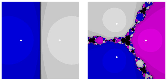
Figure 1.
Attraction basins of (27) for in left and for in right.

Figure 2.
Attraction basins of (27) for in left and for in right.
Global convergence refers to the empirical observation that the proposed iteration converges from a wide set of initial guesses, rather than to a formal global theorem valid for all starting points (except the points located on the imaginary axis). Definitively, this observation can be mathematically proven, which is why we will not pursue this in this work and in the future. To support this statement, the attraction basins of the scalar prototype have been computed over a dense grid in the complex plane for polynomial test problems of the form , as illustrated in Figure 1 and Figure 2. These visualizations show that the basins associated with the proposed method are substantially larger and more regular than those of the Padé-type competitors of the same order. However, it is clearly stated that the type of convergence for is local. The enlarged convergence regions demonstrate that the specific coefficient structure of the new iteration stabilizes its dynamics beyond the neighborhood of the root, allowing for convergence from more distant or perturbed initial values.
3.4. Computation of the MSR
The applicability of the iterative scheme introduced in (27) can be extended to the computation of MSRs by exploiting a fundamental structural identity; see [1]. Specifically, for any nonsingular matrix , the following relation holds:
We defined the block matrix . This identity provides a powerful conceptual and computational bridge between the matrix sign function and the MSR problem. It demonstrates that by embedding A into a larger block matrix of dimension , the square root of A (together with its inverse) emerges naturally as a sub-block of the matrix sign function of the extended system. Consequently, efficient iterative algorithms for the sign function can be adapted to yield both and simultaneously.
A key structural property of the proposed method becomes evident when applied to an invertible matrix A whose spectrum avoids the closed negative real axis, i.e., A has no eigenvalues in [23]. Suppose that the initial iterate is chosen such that it commutes with A, i.e.,
By induction, this commutativity is preserved for all subsequent iterates, so that
This invariance property guarantees that the spectral structure of A is respected throughout the iteration, thereby enhancing both numerical stability and theoretical tractability. Preserving commutativity also ensures that convergence analysis can be effectively reduced to the study of scalar or block structures corresponding to the spectrum of A.
Throughout this section, let be invertible with . Under this spectral condition, the principal square root and its inverse exist and are unique, and the principal logarithm is well defined. All matrix norms are subordinate and denoted by . For the sign iteration, we write , so that and is a primary matrix function of A. When analyzing the square-root computation via the block embedding (30), we use and We assume the initial iterate commutes with A; equivalently, is a primary function of A. This commutativity is preserved by rational iterations that are polynomials in and ; hence, it holds for (27)–(29) for all k.
3.5. Error Estimates and Convergence Analysis
The efficiency of the proposed iteration is underscored by its rapid convergence. The following theorem establishes its fourth-order rate of convergence toward the principal square root.
Theorem 2.
Let be invertible with , and let . Consider the iteration (27) (equivalently, (29)) with an initial matrix that commutes with A and is sufficiently close to Ω. Then, the sequence is well defined and converges to Ω with order four:
where the constant depends continuously on and on upper bounds for defined below. Moreover, applying the same iteration to the block matrix in (30) yields quartic convergence of the off-diagonal blocks to and ; hence, the MSR iteration is fourth-order under the same spectral assumption.
Proof.
Write the iteration (27) in the compact form
Let . Because satisfies and, by the commutativity hypothesis, , all polynomials in commute with . Using these relations, expand by algebraic manipulation (no series in A is required). A direct calculation yields the exact factorization
Taking norms and using submultiplicativity gives
It remains to bound the two prefactors for sufficiently close to . First, continuity of the map at ensures that there exists and such that whenever , because is invertible. Second, continuity yields for , with at the limit and a small perturbation margin. Combining these two bounds with (31), for we obtain
This proves fourth-order convergence to .
For the MSR, apply the same argument to the block matrix and the iteration with commuting with . Since and , the same calculation yields
for sufficiently close to . Quartic convergence of the full block matrix implies quartic convergence of its off-diagonal blocks to and in any subordinate norm. □
The bound in (31) provides the constructive constant with
for any radius within which remains nonsingular. Since and the spectrum depends continuously on X, such an r exists. Consequently, there is a neighborhood of in which the iteration map is well defined and contractive in the fourth power, yielding order four in the sense of .
The convergence of the proposed scheme is guaranteed under the following conditions:
- The matrix is invertible and has no eigenvalues on the closed negative real axis.
- The initial iterate commutes with A and is sufficiently close to the principal square root .
- Under these assumptions, Theorem 2 ensures global fourth-order convergence for this task.
Numerical evidence in Section 4 indicates that the basins of attraction are often large in practice, suggesting that the method enjoys a degree of global stability.
3.6. Computational Cost
Each iteration of the proposed scheme requires four matrix–matrix multiplications and one matrix inversion, leading to an overall cost of
assuming a dense arithmetic.
Table 3 compares the per-iteration complexities of representative algorithms:
Table 3.
Per-iteration cost of iterative schemes for the MSR.
Thus, the cost per iteration is comparable to Padé , but the observed iteration count is smaller, yielding overall efficiency gains.
3.7. Stability Issues
The stability of an iterative matrix algorithm is best assessed through the evolution of its residual and perturbation propagation. Let the exact fixed point of the iteration be denoted by , and let the computed iterate at step k be , where represents the accumulated roundoff or perturbation error. We analyze the error propagation by linearizing the iteration map around .
The iteration can be expressed as , where the Fréchet derivative of at governs the amplification of perturbations:
From the explicit form of ,
the derivative can be computed using standard matrix calculus and the identities , , and . After simplification, one obtains
Since for any subordinate norm, the linearized amplification factor satisfies
Hence, perturbations decay by at least a factor of per iteration in the linear regime, demonstrating that the iteration is numerically stable in the sense of backward error analysis.
Now define the residual for the matrix sign computation. From the iteration formula, we can express one full step as a rational transformation of ,
where the matrix coefficient satisfies , with C bounded as in Theorem 2. Therefore,
confirming that the residual norm decays quartically and that the method exhibits fourth-order local error reduction without explosive growth of roundoff errors.
Now let the perturbed matrix be , with . For the principal square root, the Fréchet derivative satisfies
Because the proposed method computes both and simultaneously, the ratio remains bounded for well-conditioned A. Thus, the overall numerical conditioning of the algorithm is directly inherited from that of the matrix square root itself and does not introduce additional amplification factors.
4. Numerical Results
This section presents a comprehensive numerical study designed to evaluate the performance, stability, and robustness of the iterative schemes introduced in the previous sections for computing both the MSR and its inverse. All numerical experiments were carried out using the Wolfram Mathematica 14.0 computational platform [24], executed on a uniform hardware configuration Intel Core i7-1355U (Intel Corporation, Santa Clara, CA, USA) to ensure consistency and fair comparison across the different solvers.
The evaluation encompasses several well-established iterative algorithms, namely: (13) Newt, (14) DenB, (15) CyclR, (17) PadF, (18) PadS, and (27) NewS. These algorithms are systematically compared in terms of convergence speed, numerical stability, and computational cost. Special emphasis is placed on assessing the balance between accuracy and efficiency, as these criteria are decisive in practical large-scale applications where repeated computation of matrix functions is required.
It is important to note that the existence and uniqueness of the MSR are guaranteed only for matrices whose spectra do not intersect the closed negative real axis. For non-normal, or ill-conditioned matrices that violate this condition, the MSR may not exist or may fail to be unique, making direct numerical comparison between iterative solvers inconsistent. Therefore, our experimental design focuses on classes of matrices—such as structured and symmetric positive definite (SPD) matrices—where the principal square root is well defined and unique, ensuring a fair and meaningful comparison across all tested algorithms.
To measure convergence and control termination of the iterative process, we adopt the following relative error criterion based on residuals in the -norm:
where is the prescribed tolerance. This criterion ensures that iterations halt as soon as two successive approximations become sufficiently close relative to the magnitude of the current iterate, thereby ensuring both numerical reliability and computational efficiency. Unless stated otherwise, is used throughout the experiments.
The numerical assessment does not rely on a single illustrative case; rather, it is based on a structured set of test matrices designed to capture diverse computational scenarios. Specifically, four test problems of varying dimensions are considered, thereby highlighting solver performance as the problem size grows. Each example is carefully selected to expose different spectral and structural features of the test matrices, which influence convergence behavior and numerical stability.
Example 1.

We first examine the solvers on a structured SPD matrix, inspired by tridiagonal discretizations that frequently arise in numerical analysis and engineering models. The test matrix of size is defined as
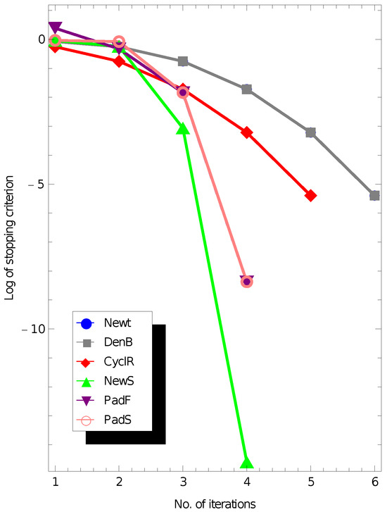
This choice ensures that A is sparse, banded, and symmetric positive definite, making it representative of discretized differential operators commonly encountered in applications. For each solver, both the square root and the inverse square root are computed simultaneously. Performance is reported with respect to iteration counts, computational time, and accuracy of the obtained approximations. The results are provided in Figure 3, Figure 4, Figure 5 and Figure 6.
Figure 3.
Results to find the MSR in Example 1, when .
Figure 4.
Results to find the MSR in Example 1, when .
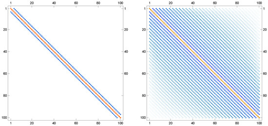
Figure 5.
Sparsity patterns of the input matrix A and its MSR in left and right, respectively, when .
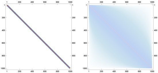
Figure 6.
Sparsity patterns of the input matrix A and its MSR in left and right, respectively, when .
Performance results confirm that the proposed solver maintains stability and accuracy in these challenging scenarios, outperforming Newton and Denman–Beavers iterations in iteration count and residual norms.
Some implementation notes are in order, including the following:
- (i)
- The iteration terminates when or when (typically ).
- (ii)
- The safeguard criterion on the residual prevents divergence for ill-scaled starting points.
- (iii)
- Each iteration requires four matrix–matrix multiplications and one matrix inversion; in large-scale implementations, the inversion may be replaced by the solution of linear systems with multiple right-hand sides.
- (iv)
- For the MSR computation, the same code can be used by embedding A into the block matrix and extracting the off-diagonal blocks after convergence.
5. Concluding Remarks
In this study, we have developed and analyzed a novel iterative framework for the simultaneous calculation of the MSR and its inverse. By exploiting the intrinsic connection between the matrix sign function and the MSR, we have proposed a fourth-order method that guarantees global convergence under suitable spectral assumptions. Theoretical analysis has confirmed the convergence order, while numerical experiments have demonstrated that the proposed algorithms have achieved superior accuracy, robustness, and computational efficiency in comparison with classical schemes such as Newton’s iteration, Denman–Beavers splitting, cyclic reduction, and Padé-based methods.
Furthermore, the proposed method has preserved important structural invariants, including commutativity with the underlying matrix, which has contributed to its numerical stability. Applications in differential equations, control theory, and risk management have highlighted the practical relevance of efficient MSR computations. The results have indicated that the introduced framework has successfully bridged theoretical insights with algorithmic effectiveness.
Future research may focus on extending the present framework to matrix pth root [25] structured matrix classes, large-scale sparse systems, and parallel computational architectures.
Author Contributions
Conceptualization, J.Z. and T.L.; methodology, J.Z., Y.L. (Yutong Li) and Q.M.; software, J.Z. and Y.L. (Yutong Li); validation, Y.L. (Yilin Li); formal analysis, J.Z. and Q.M.; investigation, J.Z. and Y.L. (Yutong Li); resources, T.L.; data curation, Y.L. (Yilin Li); writing—original draft preparation, J.Z. and Y.L. (Yutong Li); writing—review and editing, J.Z. and T.L.; visualization, Y.L. (Yutong Li); supervision, T.L. and Q.M.; project administration, T.L. and Q.M.; funding acquisition, T.L. All authors have read and agreed to the published version of the manuscript.
Funding
This research was funded by the Research Project on Graduate Education and Teaching Reform of Hebei Province of China (YJG2024133), the Open Fund Project of Marine Ecological Restoration and Smart Ocean Engineering Research Center of Hebei Province (HBMESO2321), and the Technical Service Project of Eighth Geological Brigade of Hebei Bureau of Geology and Mineral Resources Exploration (KJ2025-029, KJ2025-037).
Data Availability Statement
The data presented in this study are available on request from the corresponding author. The data are not publicly available because the research data are confidential.
Conflicts of Interest
The authors declare no conflicts of interest.
References
- Higham, N.J. Functions of Matrices: Theory and Computation; Society for Industrial and Applied Mathematics: Philadelphia, PA, USA, 2008. [Google Scholar]
- Song, Y.; Soleymani, F.; Kumar, A. Finding the geometric mean for two Hermitian matrices by an efficient iteration method, Math. Methods Appl. Sci. 2025, 48, 7188–7196. [Google Scholar] [CrossRef]
- Dehghani-Madiseh, M. On the solution of parameterized Sylvester matrix equations. J. Math. Model. 2022, 10, 535–553. [Google Scholar]
- Kenney, C.S.; Laub, A.J. The matrix sign function and computation of matrix square roots. SIAM J. Matrix Anal. Appl. 1995, 16, 980–1003. [Google Scholar]
- Deadman, E.; Higham, N.J.; Ralha, R. Blocked Schur algorithms for computing the matrix square root. Numer. Algorithms 2013, 63, 655–673. [Google Scholar]
- Zhang, K.; Soleymani, F.; Shateyi, S. On the construction of a two-step sixth-order scheme to find the Drazin generalized inverse. Axioms 2025, 14, 22. [Google Scholar] [CrossRef]
- Bini, D.A.; Higham, N.J.; Meini, B. Algorithms for the matrix pth root. Numer. Algorithms 2005, 39, 349–378. [Google Scholar] [CrossRef]
- Cheng, S.H.; Higham, N.J.; Kenney, C.S.; Laub, A.J. Approximating the logarithm of a matrix to specified accuracy. SIAM J. Matrix Anal. Appl. 2001, 22, 1112–1125. [Google Scholar] [CrossRef]
- Smith, M.I. A Schur algorithm for computing matrix pth roots. SIAM J. Matrix Anal. Appl. 2003, 24, 971–989. [Google Scholar] [CrossRef]
- Denman, E.D.; Beavers, A.N. The matrix sign function and computations in systems. Appl. Math. Comput. 1976, 2, 63–94. [Google Scholar] [CrossRef]
- Torkashvand, V. A two-step method adaptive with memory with eighth-order for solving nonlinear equations and its dynamic. Comput. Meth. Diff. Equ. 2022, 10, 1007–1026. [Google Scholar]
- Soleymani, F. An efficient twelfth-order iterative method for finding all the solutions of nonlinear equations. J. Comput. Methods Sci. Eng. 2013, 13, 309–320. [Google Scholar] [CrossRef]
- Soleymani, F. Two novel classes of two-step optimal methods for all the zeros in an interval. Afr. Mat. 2014, 25, 307–321. [Google Scholar] [CrossRef]
- Cordero, A.; Leonardo Sepúlveda, M.A.; Torregrosa, J.R. Dynamics and stability on a family of optimal fourth-order iterative methods. Algorithms 2022, 15, 387. [Google Scholar] [CrossRef]
- Higham, N.J. Newton’s method for the matrix square root. Math. Comput. 1986, 46, 537–549. [Google Scholar] [CrossRef]
- Meini, B. The Matrix Square Root from a New Functional Perspective: Theoretical Results and Computational Issues; Technical Report 1455; Dipartimento di Matematica, Università di Pisa: Pisa, Italy, 2003. [Google Scholar]
- Kenney, C.S.; Laub, A.J. Rational iterative methods for the matrix sign function. SIAM J. Matrix Anal. Appl. 1991, 12, 273–291. [Google Scholar] [CrossRef]
- Jung, D.; Chun, C. A general approach for improving the Padé iterations for the matrix sign function. J. Comput. Appl. Math. 2024, 436, 115348. [Google Scholar] [CrossRef]
- Sharma, P.; Kansal, M. An iterative formulation to compute the matrix sign function and its application in evaluating the geometric mean of Hermitian positive definite matrices. Mediterr. J. Math. 2025, 22, 39. [Google Scholar] [CrossRef]
- Cordero, A.; Rojas-Hiciano, R.V.; Torregrosa, J.R.; Vassileva, M.P. High-level convergence order accelerators of iterative methods for nonlinear problems. Appl. Numer. Math. 2025, 217, 390–411. [Google Scholar] [CrossRef]
- Rani, L.; Kansal, M. Numerically stable iterative methods for computing matrix sign function. Math. Meth. Appl. Sci. 2023, 46, 8596–8617. [Google Scholar] [CrossRef]
- Getz, C.; Helmstedt, J. Graphics with Mathematica Fractals, Julia Sets, Patterns and Natural Forms; Elsevier: Amsterdam, The Netherlands, 2004. [Google Scholar]
- Sharma, P.; Kansal, M. Extraction of deflating subspaces using disk function of a matrix pencil via matrix sign function with application in generalized eigenvalue problem. J. Comput. Appl. Math. 2024, 442, 115730. [Google Scholar] [CrossRef]
- Abell, M.L.; Braselton, J.P. Mathematica by Example, 5th ed.; Academic Press: Cambridge, MA, USA, 2017. [Google Scholar]
- Amat, S.; Busquier, S.; Hernández-Verón, M.Á.; Magreñán, Á.A. On high-order iterative schemes for the matrix pth root avoiding the use of inverses. Mathematics 2021, 9, 144. [Google Scholar] [CrossRef]


Disclaimer/Publisher’s Note: The statements, opinions and data contained in all publications are solely those of the individual author(s) and contributor(s) and not of MDPI and/or the editor(s). MDPI and/or the editor(s) disclaim responsibility for any injury to people or property resulting from any ideas, methods, instructions or products referred to in the content. |
© 2025 by the authors. Licensee MDPI, Basel, Switzerland. This article is an open access article distributed under the terms and conditions of the Creative Commons Attribution (CC BY) license (https://creativecommons.org/licenses/by/4.0/).