Fast Deep Belief Propagation: An Efficient Learning-Based Algorithm for Solving Constraint Optimization Problems

Abstract

Belief Propagation (BP) is a fundamental heuristic for solving Constraint Optimization Problems (COPs), yet its practical applicability is constrained by slow convergence and instability in loopy factor graphs. While Damped BP (DBP) improves convergence by using manually tuned damping factors, its reliance on labor-intensive hyperparameter optimization limits scalability. Deep Attentive BP (DABP) addresses this by automating damping through recurrent neural networks (RNNs), but introduces significant memory overhead and sequential computation bottlenecks. To reduce memory usage and accelerate deep belief propagation, this paper introduces Fast Deep Belief Propagation (FDBP), a deep learning framework that improves COP solving through online self-supervised learning and graphics processing unit (GPU) acceleration. FDBP decouples the learning of damping factors from BP message passing, inferring all parameters for an entire BP iteration in a single step, and leverages mixed precision to further optimize GPU memory usage. This approach substantially improves both the efficiency and scalability of BP optimization. Extensive evaluations on synthetic and real-world benchmarks highlight the superiority of FDBP, especially for large-scale instances where DABP fails due to memory constraints. Moreover, FDBP achieves an average speedup of 2.87× over DABP with the same restart counts. Because BP for COPs is a mathematically grounded GPU-parallel message-passing framework that bridges applied mathematics, computing, and machine learning, and is widely applicable across science and engineering, our work offers a promising step toward more efficient solutions to these problems.

1. Introduction

Belief Propagation (BP) [1,2] plays a pivotal role as a message-passing algorithm in graphical models. Its applications range from computing the partition function of a Markov random field [3] to estimating marginal distributions [4] and decoding low-density parity-check (LDPC) codes [5]. Constraint optimization problems (COPs) [6,7] provide a versatile mathematical framework for modeling real-world challenges in transportation, supply chain management, energy, finance, and scheduling [7,8,9,10]. In the realm of COPs, BP, also recognized as Min-sum message passing [11], seeks cost-optimal solutions by propagating cost information throughout the factor graph. Beyond standard BP, variational, bounding, and elimination-based perspectives provide additional context for inference in loopy or high-treewidth settings, including Tree-Reweighted BP (TRW) and Max-Product Linear Programming (MPLP) for bounds [12,13], as well as bucket elimination and mini-bucket approximations for structure-exploiting tradeoffs [14,15].

However, vanilla BP lacks convergence guarantees on factor graphs with loops and can converge to suboptimal fixed points in COPs with cyclic structure. Recognizing this challenge, significant research has focused on stabilizing loopy BP [16,17,18,19,20,21]. Notably, Damped Belief Propagation (DBP) [21] has gained attention for improving convergence behavior on loopy graphs. These stabilization techniques are complementary to variational and LP-based reparameterizations that control oscillation and provide certificates when available [12,13].

Despite the advantages of damping, fine-tuning damping factors per instance remains laborious. Recent work integrates deep learning to automate these choices. In particular, Deep Adaptive Belief Propagation (DABP) leverages self-supervised learning with gradient-based optimization to determine damping factors, and further introduces dynamic damping based on real-time optimization status to improve per-iteration decisions. This trend is part of a broader line on neuralized message passing that parameterizes or augments BP updates while preserving their semantics, including the Belief Propagation Neural Network (BPNN) [22], Neural-Enhanced Belief Propagation (NEBP) [23], and the Factor Graph Neural Network (FGNN) for higher-order factors [24], surveyed in learning for combinatorial reasoning and solver guidance [25].

However, DABP faces scalability and efficiency challenges, primarily due to high GPU memory consumption and its reliance on autoregressive damping-factor predictions, which limit applicability to larger instances. To address these limitations, we introduce a paradigm that decouples damping-factor learning from the BP process. By eliminating the need for a recurrent neural network (RNN) over sequential BP messages, our approach enables joint prediction of damping factors, akin to conventional deep models. This reduces the number of deep neural network (DNN) calls, yields substantial memory savings, and improves efficiency over DABP. Additionally, our method leverages mixed precision to further reduce GPU memory. We refine learning by introducing priors, constraining the damping space, and learning adaptive variations rather than directly optimizing raw values, which enhances stability and convergence. Overall, our approach substantially improves both the efficiency and scalability of DABP. Our design aligns with recent efficiency-first trends in machine learning for discrete optimization that aim to limit sequential neural computation, for example, diffusion-based solvers such as DIFUSCO and Fast tokens-to-tokens (Fast T2T) and industrial-scale pipelines like DISCO [26,27,28], as well as restart policies and learning-guided control for robust anytime behavior [29,30]. From a theoretical perspective, message-passing graph neural networks (GNNs) can capture optimal approximation algorithms for broad classes of Max-CSPs, with OptGNN providing a practical instantiation [31].

The efficacy of our algorithm is substantiated through extensive experiments across diverse benchmarks, with an emphasis on larger problem instances. Our approach not only handles significantly larger problem sizes but also achieves an average speedup of 2.87× over DABP at equivalent restart counts. In terms of solution quality, our model remains competitive for smaller instances (variable size less than 150) and surpasses baselines on larger instances, where DABP falters due to memory limitations.

Our contributions are threefold: (1) we propose FDBP, a scalable BP framework that rethinks how damping factors are learned; by leveraging online self-supervised learning and parallelizable message processing, FDBP accelerates COP solving; (2) FDBP eliminates RNN hidden-state storage and per-iteration neural passes, which reduces GPU memory usage and enables scalability to large COP instances where prior DABP fails due to memory constraints; and (3) we conduct extensive experiments across diverse benchmarks, demonstrating that FDBP achieves a favorable accuracy–efficiency tradeoff and consistent gains over existing methods.

2. Related Work

• Classical approaches to COPs. Constraint optimization problems (COPs) are NP-hard, motivating a spectrum of exact and approximate methods. Exact search includes branch-and-bound and its modern variants [32]; graphical-model based elimination (BE) and its bounded approximations via mini-buckets (MBE) provide structure-exploiting schemes with tunable accuracy–efficiency tradeoffs [14,15]. For loopy graphs, variational message passing families such as Tree-Reweighted BP (TRW) and Max-Product Linear Programming (MPLP) improve stability and provide bounds [12,13].
• Stabilizing BP on loopy factor graphs. While plain BP may oscillate or diverge on loopy graphs, damping and reparameterization can stabilize convergence. Damped BP variants for COPs demonstrate reliable convergence via adaptive damping and splitting heuristics [21]. These methods, however, still require hand-tuned hyperparameters and do not leverage learned instance structure.
• Neuralized BP and factor graph learning. Recent work integrates neural networks with factor graph inference. Belief Propagation Neural Network (BPNN) parameterizes BP updates [22]; Neural-Enhanced Belief Propagation (NEBP) augments messages with neural features while preserving BP semantics [23]. Factor Graph Neural Network (FGNN) formalizes higher-order PGMs with neuralized message passing and unrolled inference [24]. Complementing these, a survey of Cappart et al. systematizes GNNs for combinatorial reasoning and solver guidance [25]. DABP advances self-supervised damping/neighbor weighting via GRUs+GAT, improving solution quality but incurring high per-iteration compute and memory due to sequential RNN rolls [33]. Our FDBP follows this neural BP line but decouples damping inference from BP iterations, avoiding per-iteration neural passes and thus reducing memory/runtime while retaining self-supervised training.
• Neural diffusion solvers for COPs. Parallel to neuralized BP, diffusion-based graph solvers emerged as strong ML alternatives: DIFUSCO for routing [26], scalable discrete diffusion samplers for large instances, and techniques that reduce sampling cost (e.g., Fast T2T) [27]. Large-scale diffusion pipelines (e.g., DISCO) target industrial-size combinatorial problems [28]. These works likewise prioritize minimizing sequential neural computation, aligning with FDBP’s design choice to eliminate per-iteration neural overhead.
• Modern restarts and learning-guided search. Beyond classical restart theory, the recent SAT literature studies cold restarts that periodically forget parts of the solver state [29], and RL-bandit policies that adapt reset frequency online [30]. These results reinforce two of our choices: (i) using multiple restarts for robust anytime behavior and (ii) learning when/how to adjust solver dynamics without expensive inner loops.
• Theory on message passing and GNN capacity. Recent theory shows message-passing GNNs can capture optimal approximation algorithms for broad classes of Max-CSPs under standard assumptions, with practical architectures (OptGNN) realizing these guarantees [31]. This complements empirical evidence that structured, low-overhead message passing (as in FDBP) is a principled and scalable path for discrete optimization.
• Positioning. FDBP sits at the intersection of (i) stabilized BP with learned parameters and (ii) modern efficiency trends that reduce sequential neural work. Compared to DABP [33], FDBP removes per-iteration GRU/GAT passes and infers damping intermittently per restart, yielding markedly lower memory while preserving the self-supervised, label-free training setup.

3. Preliminaries

A table summarizing all acronyms and abbreviations used in the paper is provided in Appendix C.

3.1. Constraint Optimization Problems

A COP [6] can be specified by the triple $⟨X,D,F⟩$, where X is the set of variables, D collects their domains, and F is a family of cost functions. Each variable $x_i\in X$ has a finite domain $D_i\in D$. For every $f_{\mathsf{\ell }}\in F$ with scope $scp\left(f_{\mathsf{\ell }}\right)\subseteq X$, the function assigns a cost to each assignment of the variables in its scope.

The task is to compute a solution ${\tau }^{=}({\tau }^1,\dots ,{\tau }^{*}\left|X\right|)\in {\Pi }_{x_i\in X}{D}_i$ that minimizes the total cost:

$${\tau }^{*}=\underset{\tau \in {\Pi }_{x_i\in X}{D}_i}{argmin}\sum _{f_{\mathsf{\ell }}\in F}{f}_{\mathsf{\ell }}\left(\tau \right|scp\left(f\mathsf{\ell }\right)),$$

(1)

where $\tau |scp\left(f\mathsf{\ell }\right)$ denotes the restriction of $\tau$ to $scp\left(f_{\mathsf{\ell }}\right)$. A COP may be represented as a factor graph, a bipartite graph with variable nodes for elements of X and function nodes for members of F. An edge connects a variable node to a function node iff the variable belongs to the function’s scope.

3.2. Min-Sum Belief Propagation

Min-sum Belief Propagation (Min-sum BP) [11] is a standard method for COPs that runs on the factor graph representation by exchanging messages between variable and factor nodes. At iteration t, the message sent from a variable node $x_i$ to a neighboring factor $f_{\mathsf{\ell }}$ is a function $m_{x_i\to f_{\mathsf{\ell }}}^t:D_i\to \mathbb{R}$ defined as

$$m_{x_i\to f_{\mathsf{\ell }}}^t=\sum _{f_{\xi }\in \mathcal{N}i\setminus f\mathsf{\ell }}{m}_{f_{\xi }\to x_i}^{t-1},$$

(2)

where $\mathcal{N}i$ denotes the neighbors of $x_i$ in the factor graph, and $m{f_{\xi }\to x_i}^{t-1}:D_i\to \mathbb{R}$ is the message previously received by $x_i$ from $f_{\xi }$. In the opposite direction, $f_{\mathsf{\ell }}$ computes the message for $x_i$ as

$$m_{f_{\mathsf{\ell }}\to x_i}^t=\underset{\mathcal{N}\mathsf{\ell }\setminus x_i}{min}\left(f\mathsf{\ell }+\sum _{x_j\in \mathcal{N}\mathsf{\ell }\setminus x_i}{m}^{t-1}{x}_j\to f_{\mathsf{\ell }}\right).$$

(3)

After aggregating incoming messages, variable $x_i$ selects a value that minimizes its belief:

$${\tau }_i^t=\underset{{\tau }_i\in D_i}{argmin}\sum _{f_{\mathsf{\ell }}\in {\mathcal{N}}_i}{m}_{f_{\mathsf{\ell }}\to x_i}^t\left({\tau }_i\right),$$

(4)

where $m_{f_{\mathsf{\ell }}\to x_i}^t\left({\tau }_i\right)$ is the belief cost assigned to ${\tau }_i$ by the message from $f_{\mathsf{\ell }}$.

On graphs with cycles, plain Min-sum BP can exhibit non-convergence and may settle on poor solutions due to repeated influence along loops. DBP [21] mitigates these issues by damping the variable-to-factor messages. Concretely, the message from $x_i$ to $f_{\mathsf{\ell }}$ is updated as

$$m_{x_i\to f_{\mathsf{\ell }}}^t=\lambda m_{x_i\to f_{\mathsf{\ell }}}^{t-1}+(1-\lambda )\sum _{f_{\xi }\in \mathcal{N}i\setminus f\mathsf{\ell }}{m}_{f_{\xi }\to x_i}^{t-1}.$$

(5)

With an appropriate choice of $\lambda \in (0,1]$, DBP often improves both convergence behavior and the quality achieved by the undamped Min-sum BP.

4. Methodologies

In each step, the DBP algorithm uses a fixed, manually chosen damping factor to balance the contribution of new and old messages when updating the message from a variable node to a function node in a factor graph. However, the new message is composed of messages received from the neighboring function nodes of the current variable node, and the importance of these messages can vary. To address this limitation, a more flexible approach should allow for the assignment of variable-specific damping factors and neighbor-specific weights for each variable node during the BP process. Specifically, dynamic damping factors and neighbor-specific weights can be integrated into the BP process. In step t, a variable node $x_i$ computes the message to function node $f_{\mathsf{\ell }}$ using the following expression:

$$\begin{array}{cc}\hfill m_{x_i\to f_{\mathsf{\ell }}}^t& ={\lambda }_{i\to \mathsf{\ell }}^t{m}_{x_i\to f_{\mathsf{\ell }}}^{t-1}+(1-{\lambda }_{i\to \mathsf{\ell }}^t)\left(\right|{\mathcal{N}}_i|-1)\hfill \\ \hfill & \times \sum _{f_{\xi }\in {\mathcal{N}}_i\setminus \left\{f_{\mathsf{\ell }}\right\}}{w}_{\xi \to i}^t\left(\mathsf{\ell }\right)m_{f_{\xi }\to x_i}^{t-1}.\hfill \end{array}$$

(6)

Here, ${\lambda }_{i\to \mathsf{\ell }}^t\in [0,1]$ and $w_{\xi \to i}^t\left(\mathsf{\ell }\right)\in [0,1]$ represent learnable damping factors and neighbor weights, respectively, for the message from $x_i$ to $f_{\mathsf{\ell }}$ at iteration t.

Suppose a problem instance has N variables, and its corresponding factor graph has an average node degree of M. If the BP process runs for T steps until termination, the complexity of updating the factors in adaptive BP is $O\left(NMT\right)$. This represents a computationally demanding task, making manual handcrafting impractical.

In response, DABP [33] was proposed, leveraging DNNs parameterized by ${\mathcal{M}}_{\theta }$ to automatically infer these factors in an autoregressive manner:

$$w^t,{\lambda }^t={\mathcal{M}}_{\theta }\left(G,m_{x\to f}^{1:t-1},m_{f\to x}^{1:t-1}\right).$$

(7)

Here, G represents the factor graph, and $m_{x\to f}^{1:t-1}$ and $m_{f\to x}^{1:t-1}$ denote the BP messages from variable nodes to function nodes and from function nodes to variable nodes in the previous steps, respectively.

However, the entire DABP procedure operates autoregressively, requiring the invocation of DNNs at each step to infer damping factors and neighbor weights. This recurrent dependency on DNNs can significantly increase computational overhead.

4.1. Fast Deep Belief Propagation

We propose an efficient learning-based algorithm for solving constraint optimization problems, referred to as Fast Deep Belief Propagation (FDBP). An illustration of the proposed approach is provided in Figure 1. The algorithm will execute R iterations, effectively restarting R times. The restart policy has demonstrated significant potential in addressing COPs [34]. Researchers have observed that combinatorial search algorithms often exhibit highly unpredictable runtime and solution quality across problem instances. By incorporating a restart policy, the algorithm minimizes the risk of getting trapped in local minima, thereby improving its overall efficiency and effectiveness.

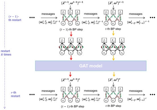
Figure 1. The workflow of our algorithm FDBP.

In each iteration r, the algorithm runs for T steps. At each step t, it updates messages ${(m_{x\to f}^t,m_{f\to x}^t)}^r$ by using the messages from the previous step ${(m_{x\to f}^{t-1},m_{f\to x}^{t-1})}^r$ and inferred parameters ${({\lambda }^t,w^t)}^r$. These parameters ${({\lambda }^t,w^t)}^r$ are computed by a Graph Attention Neural Network (GAT), which takes as input the factor graph and the messages from the previous iteration, specifically ${(m_{x\to f}^{t-1},m_{f\to x}^{t-1})}^{r-1}$.

This design introduces a key improvement: instead of inferring parameters ${({\lambda }^t,w^t)}^r$ at each step t during the current iteration (as in the DABP algorithm), our approach infers all parameters for the entire iteration r in a single step, using a single invocation of the GAT. By doing so, the algorithm avoids the need to repeatedly invoke DNNs $T-1$ times per iteration, as required in DABP. This significantly reduces computational overhead and leverages GPU parallelism, making our approach far more efficient while retaining the effectiveness of parameter inference.

The time complexity of our algorithm per iteration matches that of DBP in the worst-case scenario. However, in practice, our approach often achieves faster performance due to its enhanced convergence behavior (as demonstrated in Table 1 and Table 2 of Section 5), which reduces the required number of steps to reach convergence. Compared to DABP, our algorithm’s efficiency advantage becomes particularly evident when employing the same restart strategy, as all parameters for an entire iteration are computed simultaneously, significantly streamlining the process.

It is worth noting that our algorithm adopts a different approach to parameter inference compared to DABP. In DABP, the parameters for step t are inferred autoregressively by utilizing messages from all preceding steps (0 to $t-1$) within the same iteration, where a RNN is used to encode these messages. By contrast, our algorithm infers parameters for step using only the corresponding messages from the previous iteration, ${(m_{x\to f}^{t-1},m_{f\to x}^{t-1})}^{r-1}$. This design assumes that the messages from step t of the previous iteration already encapsulate the relevant information from earlier steps. While not directly intervening in the BP process, this approach simplifies the inference process and complements our algorithm’s overall focus on efficiency and scalability.

In summary, our FDBP introduces a significantly more efficient and scalable framework for parameter inference in learning-based belief propagation. By addressing the computational bottlenecks inherent in DABP, our approach enhances both the speed and scalability of solving COPs. Specifically, FDBP overcomes the limitations of DABP by reducing the need for repeated, computationally expensive deep learning network invocations at each iteration, thereby lowering memory overhead and avoiding sequential computation bottlenecks. This leads to improved overall performance, making it well-suited for real-world, large-scale applications where both memory efficiency and computational speed are critical.

4.2. The FDBP Algorithm

The GAT model in our FDBP algorithm is trained using an online self-supervised learning approach, removing the dependency on labor-intensive, human-labeled datasets. This design allows our method to be directly applied to solving COPs without requiring prior model pretraining. Specifically, at each iteration t, given the BP messages m, we optimize the following self-supervised objective $L\left(m\right)$:

$$\underset{\theta }{min}\mathcal{L}\left(m\right)=\sum _{f_{\mathsf{\ell }}\in F}\left(\sum _{\begin{array}{c}⟨{\tau }_{i_1},\dots ,{\tau }_{i_n}⟩\\ \in {\Pi }_{x_i\in scp\left(f_{\mathsf{\ell }}\right)}{D}_i\end{array}}{f}_{\mathsf{\ell }}({\tau }_{i_1},\dots ,{\tau }_{i_n})\prod _{j=1:n}{p}_{i_j}^t\left({\tau }_{i_j}\right)\right),$$

(8)

where $p_i\left({\tau }_{i_j}\right)$ denotes the belief-induced probability of the event $x_i={\tau }_{i_j}$, defined by the following:

$$\begin{array}{cc}\hfill p_i\left({\tau }_{i_j}\right)& ={\displaystyle \frac{exp(-b_i\left({\tau }_{i_j}\right))}{{\sum }_{{\tau }_{i_j}^{\prime }\in D_i}exp(-b_i\left({\tau }_{i_j}^{\prime }\right))}},\hfill \\ \hfill b_i\left({\tau }_{i_j}\right)& =\sum _{f_{\mathsf{\ell }}\in F_i}{m}_{f_{\mathsf{\ell }}\to x_i}\left({\tau }_{i_j}\right).\hfill \end{array}$$

Intuitively, an assignment ${\tau }_{i_j}$ is assigned a higher probability $p_i\left({\tau }_{i_j}\right)$ when it has a lower belief cost $b_i\left({\tau }_{i_j}\right)$. It preserves the minimization semantics of the argmin in Equation (4) and is consistent with the global objective in Equation (1). By leveraging this self-supervised loss, our algorithm adaptively refines its predictions in a principled manner, facilitating efficient and effective training.

Our FDBP algorithm is presented in Algorithm 1. The algorithm runs for R iterations (lines 3–19), with each iteration comprising the following steps:

• Initialization: initialize messages and parameters for the factor graph (line 4).
• Message Updates: perform sequential message updates using Equations (6) and (3) with the inferred parameters ${\lambda }^t,w^t$ (lines 6–7).
• Solution Evaluation: periodically evaluate the current solution ${\tau }^t$ and compare its cost to the best solution ${\tau }^{*}$ found so far (lines 8–10).
• Buffer Storage: store selected message pairs in a buffer for loss computation and gradient updates (lines 11–12).
• Adaptive Optimization: optimize parameters adaptively through backpropagation using the stored messages and the defined loss function (lines 15–19).

Note that we use mixed precision to further economize GPU memory and refine the learning process by constraining damping factors within the range of 0.8 to 1.0. In a departure from conventional methodologies, we learn varying factors instead of directly optimizing damping factors, aligning with empirical observations suggesting optimal values around 0.9, as noted by [21].

Algorithm 1: The fast deep belief propagation algorithm

4.3. Time Complexity

We denote by b the maximum scope size of a factor, d the maximum variable domain size, and e the average degree of a variable node in the factor graph. Let $\mathcal{M}$ be the cost of one call to the GAT-based controller (a single forward pass). We follow the implementation setting where factors and variables are processed in parallel on a single GPU; the expressions below therefore reflect wall-time under this parallelism (work complexity would multiply by $\left|F\right|$ or $\left|X\right|$ accordingly).

• Factor-to-variable update Equation (3). Evaluating a factor message over a scope of size b requires iterating over assignments of the other $b-1$ variables, giving $O\left(d^{b-1}\right)$.
• Loss/objective evaluation Equation (8). Dominated by factor evaluations; with factors processed in parallel on GPU, the wall-time is $O\left(d^{b-1}\right)$.
• Variable-to-factor (weighted BP) update Equation (6). Aggregation over the e incoming messages yields $O\left(e\right)$ (variables processed in parallel).
• Decoding Equation (4). Selecting the best label for one variable is $O\left(d\right)$ (variables processed in parallel).

Per BP iteration, the dominant cost is, therefore,

$$C_{\mathrm{iter}}=O\left(d^{b-1}+e+d\right).$$

Our controller (GAT) is invoked once every K iterations, so each restart performs $\frac{T}{K}$ controller calls, contributing $O\left(\frac{T}{K}\mathcal{M}\right)$. We evaluate the objective once per restart, adding $O\left(d^{b-1}\right)$.

• Total time complexity. With R restarts and at most T BP iterations per restart, the total wall-time is

  $$T_{\mathrm{total}}=O\left(R\left[T(d^{b-1}+e+d)+\frac{T}{K}\mathcal{M}+d^{b-1}\right]\right).$$

For methods that infer weights/damping every iteration (e.g., DABP), replace $\frac{T}{K}\mathcal{M}$ with $T\mathcal{M}$, which explains the higher per-iteration compute/memory footprint relative to our interval/restart-level controller.

5. Empirical Evaluations

In this section, we present a comprehensive empirical study on the effectiveness of our proposed FDBP. We commence by providing insights into the experimental setup and implementation details. Subsequently, we showcase the superiority of FDBP over existing state-of-the-art methods.

Benchmarks and Baselines. We evaluate on four canonical benchmarks: random COPs, scale-free networks, small-world networks, and Weighted Graph Coloring Problems (WGCPs) [7]. For random COPs and WGCPs, constraint edges are sampled i.i.d. with graph density $p_1\in (0,1]$. Scale-free instances are generated using the Barabási–Albert (BA) model with parameters $m_0,m_1\in {\mathbb{Z}}_{+}$. Small-world instances follow the Newman–Watts–Strogatz construction with $k\in {\mathbb{Z}}_{+}$ and $p\in [0,1]$. See Cohen et al. [21] for further details on problem instance generation.

We benchmark FDBP against state-of-the-art solvers for COPs: (1) Toulbar2 with a timeout of 1200 s (7200s for large-scale problems); (2) Mini-bucket Elimination (MBE) with an i-bound of 8 (i-bound of 7 for specific random COPs); (3) GAT-PCM-LNS with a destroy probability of 0.2; (4) DBP with a damping factor of 0.9 and a splitting ratio of 0.95; and (5) DABP with different restarts.

All experiments are conducted on a server equipped with an Intel(R) Xeon(R) Gold 6148 CPU (Intel Corporation, Santa Clara, CA, USA), NVIDIA GeForce RTX 3090 GPUs (NVIDIA Corporation, Santa Clara, CA, USA), and 125 GB memory. The reported results represent the best solution cost for each run, and for each experiment, the results are averaged over 100 random problem instances. For larger-scale problems, a 2-hour runtime limit is imposed on all methods.

Implementation. Our FDBP model first applies a learned linear projection to a batch of BP messages to obtain 8-dimensional embeddings. These embeddings are then processed by a stack of four Graph Attention Network (GAT) layers. Each GAT layer produces eight feature channels using four attention heads. In line with DBP and DABP, we operate on a Splitting Constraint Factor Graph (SCFG) with a splitting ratio of 0.95. The implementation is built in PyTorch Geometric and trained with the Adam optimizer, using a learning rate of ${10}^{-3}$ and weight decay $5\times {10}^{-5}$. For each problem instance, we allocate $R=20$ independent restarts and cap message passing at $T=1000$ iterations per restart (the restart budget and iteration cap were selected via a small grid search on random COPs with $\left|X\right|=100$, sweeping $R\in \{5,10,20,30\}$ and $T\in \{500,1000,1500\}$. The best trade-off between accuracy and efficiency was achieved at $R=20$ and $T=1000$, with only minor gains beyond $R=20$). Dynamic weights and damping factors are re-estimated from the current BP messages every $K=20$ iterations for most settings; for random COPs with $\left|X\right|=300$, the update schedule is tightened to every $K=10$ iterations. We provide a list of parameters used in Appendix B.

Performance Comparison. Table 1 and Table 2 compare the performance of various methods across four standard benchmarks. Table 1 focuses on smaller problem instances, while Table 2 addresses larger problem instances.

Table 1. Comparison of methods using normalised cost and relative gap. Cost is per constraint $\left|F\right|$. Gap is $(\mathrm{Cost}-{\mathrm{Cost}}_{min})/{\mathrm{Cost}}_{min}$ with lower values preferred. Best results are highlighted in both bold and blue. OOM means out of memory.

Random COPs $({\mathit{p}}_1=0.25)$
	$\left|\mathit{X}\right|=\mathbf{60}$			$\left|\mathit{X}\right|=\mathbf{80}$			$\left|\mathit{X}\right|=\mathbf{100}$
Methods	Cost	Gap	Time	Cost	Gap	Time	Cost	Gap	Time
Toulbar2	29.17	7.53%	20m	32.32	7.75%	20m	34.31	7.19%	20m
MBE	32.42	19.51%	21s	34.94	16.50%	41s	36.86	15.14%	59s
GAT-PCM-LNS	28.03	3.31%	4m35s	30.81	2.72%	10m9s	32.78	2.41%	19m23s
DBP	27.62	1.80%	38s	30.41	1.39%	1m30s	32.45	1.37%	2m45s
DABP ($R=5$)	27.21	0.28%	57s	30.10	0.35%	1m8s	32.09	0.25%	1m25s
DABP ($R=10$)	27.17	0.14%	1m53s	30.05	0.19%	2m15s	32.04	0.09%	2m56s
DABP ($R=20$)	27.13	0.00%	3m36s	29.99	0.00%	4m23s	32.01	0.00%	5m44s
FDBP ($R=5$)	27.24	0.42%	17s	30.13	0.45%	29s	32.08	0.23%	53s
FDBP ($R=10$)	27.22	0.32%	32s	30.08	0.29%	55s	32.05	0.14%	1m48s
FDBP ($R=20$)	27.17	0.14%	1m1s	30.06	0.21%	1m43s	32.02	0.03%	3m42s
WGCPs $(p_1=0.25)$
Toulbar2	0.19	0.00%	20m	1.19	36.70%	20m	2.09	41.14%	20m
MBE	2.04	1001.03%	0s	2.86	227.35%	0s	3.50	136.26%	0s
GAT-PCM-LNS	0.52	182.02%	44s	1.17	34.10%	2m5s	1.78	19.84%	3m28s
DBP	0.42	126.52%	0m17s	1.06	21.08%	1m12s	1.68	13.72%	2m55s
DABP ($R=5$)	0.32	70.94%	1m43s	0.90	2.49%	2m53s	1.59	7.55%	5m38s
DABP ($R=10$)	0.30	63.29%	3m25s	0.88	0.95%	5m35s	1.49	0.80%	11m10s
DABP ($R=20$)	0.29	55.07%	6m35s	0.87	0.00%	11m8s	1.48	0.00%	22m17s
FDBP ($R=5$)	0.33	79.84%	31s	0.90	3.23%	1m	1.51	1.65%	2m56s
FDBP ($R=10$)	0.32	73.69%	1m3s	0.89	1.47%	1m59s	1.50	0.96%	5m35s
FDBP ($R=20$)	0.31	69.37%	2m1s	0.88	0.47%	3m57s	1.49	0.32%	11m9s
Scale-free networks $(m_0=m_1=10)$
Toulbar2	30.90	7.21%	20m	31.64	8.01%	20m	32.34	9.24%	20m
MBE	33.97	17.87%	22s	34.55	17.95%	31s	34.84	17.69%	40s
GAT-PCM-LNS	29.72	3.11%	5m28s	30.41	3.82%	8m48s	31.10	5.06%	13m25s
DBP	29.28	1.60%	41s	29.79	1.70%	1m	30.03	1.43%	1m29s
DABP ($R=5$)	28.90	0.29%	1m1s	29.39	0.33%	1m3s	29.69	0.30%	1m5s
DABP ($R=10$)	28.86	0.12%	1m58s	29.34	0.16%	2m4s	29.63	0.11%	2m6s
DABP ($R=20$)	28.82	0.00%	3m50s	29.29	0.00%	4m17s	29.60	0.00%	4m12s
FDBP ($R=5$)	28.97	0.52%	14s	29.45	0.53%	19s	29.78	0.61%	23s
FDBP ($R=10$)	28.92	0.36%	28s	29.42	0.46%	36s	29.74	0.47%	48s
FDBP ($R=20$)	28.90	0.29%	54s	29.39	0.34%	1m14s	29.70	0.35%	1m34s
Small-world networks $(k=10,p=0.3)$
Toulbar2	28.51	11.01%	20m	28.80	12.37%	20m	28.37	10.67%	20m
MBE	29.46	14.69%	16s	29.40	14.73%	22s	29.31	14.32%	28s
GAT-PCM-LNS	26.49	3.13%	3m24s	26.43	3.14%	5m6s	26.26	2.45%	7m19s
DBP	25.87	0.70%	35s	25.88	0.99%	56s	25.68	0.16%	1m17s
DABP ($R=5$)	25.77	0.33%	1m52s	25.71	0.34%	1m39s	25.73	0.35%	2m
DABP ($R=10$)	25.72	0.13%	3m42s	25.67	0.16%	3m18s	25.67	0.12%	3m57s
DABP ($R=20$)	25.69	0.00%	7m18s	25.63	0.00%	6m33s	25.64	0.00%	7m57s
FDBP ($R=5$)	25.81	0.49%	20s	25.75	0.47%	31s	25.75	0.46%	41s
FDBP ($R=10$)	25.76	0.27%	40s	25.68	0.22%	1m4s	25.71	0.28%	1m19s
FDBP ($R=20$)	25.72	0.11%	1m18s	25.63	0.02%	2m5s	25.67	0.14%	2m34s

Table 1. Comparison of methods using normalised cost and relative gap. Cost is per constraint $\left|F\right|$. Gap is $(\mathrm{Cost}-{\mathrm{Cost}}_{min})/{\mathrm{Cost}}_{min}$ with lower values preferred. Best results are highlighted in both bold and blue. OOM means out of memory.

Random COPs $({\mathit{p}}_1=0.25)$
	$\left|\mathit{X}\right|=\mathbf{60}$			$\left|\mathit{X}\right|=\mathbf{80}$			$\left|\mathit{X}\right|=\mathbf{100}$
Methods	Cost	Gap	Time	Cost	Gap	Time	Cost	Gap	Time
Toulbar2	29.17	7.53%	20m	32.32	7.75%	20m	34.31	7.19%	20m
MBE	32.42	19.51%	21s	34.94	16.50%	41s	36.86	15.14%	59s
GAT-PCM-LNS	28.03	3.31%	4m35s	30.81	2.72%	10m9s	32.78	2.41%	19m23s
DBP	27.62	1.80%	38s	30.41	1.39%	1m30s	32.45	1.37%	2m45s
DABP ($R=5$)	27.21	0.28%	57s	30.10	0.35%	1m8s	32.09	0.25%	1m25s
DABP ($R=10$)	27.17	0.14%	1m53s	30.05	0.19%	2m15s	32.04	0.09%	2m56s
DABP ($R=20$)	27.13	0.00%	3m36s	29.99	0.00%	4m23s	32.01	0.00%	5m44s
FDBP ($R=5$)	27.24	0.42%	17s	30.13	0.45%	29s	32.08	0.23%	53s
FDBP ($R=10$)	27.22	0.32%	32s	30.08	0.29%	55s	32.05	0.14%	1m48s
FDBP ($R=20$)	27.17	0.14%	1m1s	30.06	0.21%	1m43s	32.02	0.03%	3m42s
WGCPs $(p_1=0.25)$
Toulbar2	0.19	0.00%	20m	1.19	36.70%	20m	2.09	41.14%	20m
MBE	2.04	1001.03%	0s	2.86	227.35%	0s	3.50	136.26%	0s
GAT-PCM-LNS	0.52	182.02%	44s	1.17	34.10%	2m5s	1.78	19.84%	3m28s
DBP	0.42	126.52%	0m17s	1.06	21.08%	1m12s	1.68	13.72%	2m55s
DABP ($R=5$)	0.32	70.94%	1m43s	0.90	2.49%	2m53s	1.59	7.55%	5m38s
DABP ($R=10$)	0.30	63.29%	3m25s	0.88	0.95%	5m35s	1.49	0.80%	11m10s
DABP ($R=20$)	0.29	55.07%	6m35s	0.87	0.00%	11m8s	1.48	0.00%	22m17s
FDBP ($R=5$)	0.33	79.84%	31s	0.90	3.23%	1m	1.51	1.65%	2m56s
FDBP ($R=10$)	0.32	73.69%	1m3s	0.89	1.47%	1m59s	1.50	0.96%	5m35s
FDBP ($R=20$)	0.31	69.37%	2m1s	0.88	0.47%	3m57s	1.49	0.32%	11m9s
Scale-free networks $(m_0=m_1=10)$
Toulbar2	30.90	7.21%	20m	31.64	8.01%	20m	32.34	9.24%	20m
MBE	33.97	17.87%	22s	34.55	17.95%	31s	34.84	17.69%	40s
GAT-PCM-LNS	29.72	3.11%	5m28s	30.41	3.82%	8m48s	31.10	5.06%	13m25s
DBP	29.28	1.60%	41s	29.79	1.70%	1m	30.03	1.43%	1m29s
DABP ($R=5$)	28.90	0.29%	1m1s	29.39	0.33%	1m3s	29.69	0.30%	1m5s
DABP ($R=10$)	28.86	0.12%	1m58s	29.34	0.16%	2m4s	29.63	0.11%	2m6s
DABP ($R=20$)	28.82	0.00%	3m50s	29.29	0.00%	4m17s	29.60	0.00%	4m12s
FDBP ($R=5$)	28.97	0.52%	14s	29.45	0.53%	19s	29.78	0.61%	23s
FDBP ($R=10$)	28.92	0.36%	28s	29.42	0.46%	36s	29.74	0.47%	48s
FDBP ($R=20$)	28.90	0.29%	54s	29.39	0.34%	1m14s	29.70	0.35%	1m34s
Small-world networks $(k=10,p=0.3)$
Toulbar2	28.51	11.01%	20m	28.80	12.37%	20m	28.37	10.67%	20m
MBE	29.46	14.69%	16s	29.40	14.73%	22s	29.31	14.32%	28s
GAT-PCM-LNS	26.49	3.13%	3m24s	26.43	3.14%	5m6s	26.26	2.45%	7m19s
DBP	25.87	0.70%	35s	25.88	0.99%	56s	25.68	0.16%	1m17s
DABP ($R=5$)	25.77	0.33%	1m52s	25.71	0.34%	1m39s	25.73	0.35%	2m
DABP ($R=10$)	25.72	0.13%	3m42s	25.67	0.16%	3m18s	25.67	0.12%	3m57s
DABP ($R=20$)	25.69	0.00%	7m18s	25.63	0.00%	6m33s	25.64	0.00%	7m57s
FDBP ($R=5$)	25.81	0.49%	20s	25.75	0.47%	31s	25.75	0.46%	41s
FDBP ($R=10$)	25.76	0.27%	40s	25.68	0.22%	1m4s	25.71	0.28%	1m19s
FDBP ($R=20$)	25.72	0.11%	1m18s	25.63	0.02%	2m5s	25.67	0.14%	2m34s

Table 2. Comparison of methods using normalised cost and relative gap. Cost is per constraint $\left|F\right|$. Gap is $(\mathrm{Cost}-{\mathrm{Cost}}_{min})/{\mathrm{Cost}}_{min}$ with lower values preferred. Best results are highlighted in both bold and blue. OOM means out of memory.

Random COPs $({\mathit{p}}_1=0.25)$
	$\left|\mathit{X}\right|=\mathbf{150}$			$\left|\mathit{X}\right|=\mathbf{200}$			$\left|\mathit{X}\right|=\mathbf{250}$			$\left|\mathit{X}\right|=\mathbf{300}$
Methods	Cost	Gap	Time	Cost	Gap	Time	Cost	Gap	Time	Cost	Gap	Time
Toulbar2	37.16	5.49%	2h	38.92	4.69%	2h	40.14	4.27%	2h	41.05	3.90%	2h
MBE	39.48	12.057%	2m32s	41.00	10.29%	4m40s	41.98	9.03%	27s	42.71	8.09%	40s
GAT-PCM-LNS	35.86	1.81%	1h5m	37.86	1.84%	2h	39.32	2.13%	2h	40.39	2.22%	2h
DBP	35.56	0.96%	9m50s	37.50	0.87%	22m38s	38.76	0.67%	45m43s	39.73	0.57%	1h90m
DABP ($R=5$)
DABP ($R=10$)	OOM			OOM			OOM			OOM
DABP ($R=20$)
FDBP ($R=5$)	35.30	0.21%	2m7s	37.23	0.14%	3m53s	38.54	0.12%	4m25s	39.55	0.10%	5m10s
FDBP ($R=10$)	35.26	0.10%	4m19s	37.20	0.07%	7m42s	38.52	0.06%	8m44s	39.53	0.06%	10m24s
FDBP ($R=20$)	35.23	0.00%	8m47s	37.18	0.00%	15m11s	38.50	0.00%	17m17s	39.51	0.00%	20m54s
WGCPs $(p_1=0.25)$
Toulbar2	3.43	25.83%	20m	4.25	17.89%	2h	4.88	14.73%	2h	5.36	11.61%	2h
MBE	4.55	66.84%	1s	5.20	44.15%	1s	5.70	34.07%	2s	6.06	26.22%	3s
GAT-PCM-LNS	2.97	9.04%	10m39s	3.78	4.70%	22m1s	4.37	2.84%	41m49s	4.81	0.31%	1h8m
DBP	3.00	10.08%	11m42s	4.01	11.05%	27m54s	4.71	10.79%	53m48s	5.24	9.14%	1h42m
DABP($R=5$)
DABP ($R=10$)	OOM			OOM			OOM			OOM
DABP ($R=20$)
FDBP ($R=5$)	2.79	2.53%	5m48s	3.70	2.42%	11m43s	4.38	3.00%	18m54s	4.99	3.89%	24m57s
FDBP ($R=10$)	2.75	0.78%	11m32s	3.64	1.01%	23m17s	4.31	1.22%	38m9s	4.89	1.94%	50m
FDBP ($R=20$)	2.73	0.00%	23m18s	3.61	0.00%	46m15s	4.25	0.00%	1h16m	4.80	0.00%	1h40m
Scale-free networks $(m_0=m_1=10)$
Toulbar2	33.09	10.27%	20m	33.07	9.12%	2h	33.18	8.81%	2h	33.45	9.50%	2h
MBE	35.26	17.48%	1m3s	35.40	16.79%	1m25s	35.51	16.46%	1m51s	35.65	16.71%	2m18s
GAT-PCM-LNS	32.32	7.68%	30m46s	33.27	9.76%	53m15s	33.79	10.82%	1h20m	34.26	12.14%	1h54m
DBP	30.36	1.17%	2m34s	30.59	0.93%	4m9s	30.69	0.65%	5m15s	30.78	0.74%	6m29s
DABP($R=5$)	30.08	0.23%	1m14s
DABP ($R=10$)	30.04	0.11%	2m23s	OOM			OOM			OOM
DABP ($R=20$)	30.01	0.00%	4m41s
FDBP ($R=5$)	30.14	0.43%	36s	30.38	0.23%	36s	30.53	0.13%	47s	30.59	0.12%	47s
FDBP ($R=10$)	30.11	0.32%	1m8s	30.33	0.08%	1m10s	30.52	0.08%	1m33s	30.57	0.06%	1m34s
FDBP ($R=20$)	30.08	0.22%	2m10s	30.31	0.00%	2m21s	30.49	0.00%	3m4s	30.55	0.00%	3m10s
Small-world networks $(k=10,p=0.3)$
Toulbar2	28.16	12.66%	20m	28.77	12.13%	20m	27.95	8.80%	2h	27.74	8.06%	2h
MBE	28.47	13.90%	42s	29.29	14.17%	55s	29.87	16.26%	1m9s	29.63	15.43%	1m23s
GAT-PCM-LNS	25.66	2.65%	14m41s	26.32	2.60%	22m50s	26.91	4.74%	32m56s	26.65	3.84%	45m3s
DBP	25.00	0.00%	2m49s	25.66	0.00%	4m24s	26.18	1.89%	6m31	25.95	1.10%	8m20s
DABP ($R=5$)	25.73	2.92%	3m5s	25.74	0.31%	3m50s	25.76	0.28%	4m52s	25.73	0.24%	5m40s
DABP ($R=10$)	25.69	2.77%	6m6s	25.69	0.14%	7m36s	25.73	0.15%	9m59s	25.69	0.09%	11m27s
DABP ($R=20$)	25.65	2.60%	12m28s	25.66	0.01%	14m54s	25.69	0.00%	19m57s	25.67	0.00%	22m56s
FDBP ($R=5$)	25.75	3.01%	1m4s	25.77	0.42%	1m44s	25.79	0.39%	3m5s	25.77	0.41%	2m55s
FDBP ($R=10$)	25.70	2.83%	2m7s	25.72	0.22%	3m35s	25.75	0.22%	6m1s	25.74	0.29%	5m49s
FDBP ($R=20$)	25.67	2.69%	4m18s	25.68	0.08%	7m6s	25.72	0.12%	11m49s	25.71	0.15%	11m22s

Table 2. Comparison of methods using normalised cost and relative gap. Cost is per constraint $\left|F\right|$. Gap is $(\mathrm{Cost}-{\mathrm{Cost}}_{min})/{\mathrm{Cost}}_{min}$ with lower values preferred. Best results are highlighted in both bold and blue. OOM means out of memory.

Random COPs $({\mathit{p}}_1=0.25)$
	$\left|\mathit{X}\right|=\mathbf{150}$			$\left|\mathit{X}\right|=\mathbf{200}$			$\left|\mathit{X}\right|=\mathbf{250}$			$\left|\mathit{X}\right|=\mathbf{300}$
Methods	Cost	Gap	Time	Cost	Gap	Time	Cost	Gap	Time	Cost	Gap	Time
Toulbar2	37.16	5.49%	2h	38.92	4.69%	2h	40.14	4.27%	2h	41.05	3.90%	2h
MBE	39.48	12.057%	2m32s	41.00	10.29%	4m40s	41.98	9.03%	27s	42.71	8.09%	40s
GAT-PCM-LNS	35.86	1.81%	1h5m	37.86	1.84%	2h	39.32	2.13%	2h	40.39	2.22%	2h
DBP	35.56	0.96%	9m50s	37.50	0.87%	22m38s	38.76	0.67%	45m43s	39.73	0.57%	1h90m
DABP ($R=5$)
DABP ($R=10$)	OOM			OOM			OOM			OOM
DABP ($R=20$)
FDBP ($R=5$)	35.30	0.21%	2m7s	37.23	0.14%	3m53s	38.54	0.12%	4m25s	39.55	0.10%	5m10s
FDBP ($R=10$)	35.26	0.10%	4m19s	37.20	0.07%	7m42s	38.52	0.06%	8m44s	39.53	0.06%	10m24s
FDBP ($R=20$)	35.23	0.00%	8m47s	37.18	0.00%	15m11s	38.50	0.00%	17m17s	39.51	0.00%	20m54s
WGCPs $(p_1=0.25)$
Toulbar2	3.43	25.83%	20m	4.25	17.89%	2h	4.88	14.73%	2h	5.36	11.61%	2h
MBE	4.55	66.84%	1s	5.20	44.15%	1s	5.70	34.07%	2s	6.06	26.22%	3s
GAT-PCM-LNS	2.97	9.04%	10m39s	3.78	4.70%	22m1s	4.37	2.84%	41m49s	4.81	0.31%	1h8m
DBP	3.00	10.08%	11m42s	4.01	11.05%	27m54s	4.71	10.79%	53m48s	5.24	9.14%	1h42m
DABP($R=5$)
DABP ($R=10$)	OOM			OOM			OOM			OOM
DABP ($R=20$)
FDBP ($R=5$)	2.79	2.53%	5m48s	3.70	2.42%	11m43s	4.38	3.00%	18m54s	4.99	3.89%	24m57s
FDBP ($R=10$)	2.75	0.78%	11m32s	3.64	1.01%	23m17s	4.31	1.22%	38m9s	4.89	1.94%	50m
FDBP ($R=20$)	2.73	0.00%	23m18s	3.61	0.00%	46m15s	4.25	0.00%	1h16m	4.80	0.00%	1h40m
Scale-free networks $(m_0=m_1=10)$
Toulbar2	33.09	10.27%	20m	33.07	9.12%	2h	33.18	8.81%	2h	33.45	9.50%	2h
MBE	35.26	17.48%	1m3s	35.40	16.79%	1m25s	35.51	16.46%	1m51s	35.65	16.71%	2m18s
GAT-PCM-LNS	32.32	7.68%	30m46s	33.27	9.76%	53m15s	33.79	10.82%	1h20m	34.26	12.14%	1h54m
DBP	30.36	1.17%	2m34s	30.59	0.93%	4m9s	30.69	0.65%	5m15s	30.78	0.74%	6m29s
DABP($R=5$)	30.08	0.23%	1m14s
DABP ($R=10$)	30.04	0.11%	2m23s	OOM			OOM			OOM
DABP ($R=20$)	30.01	0.00%	4m41s
FDBP ($R=5$)	30.14	0.43%	36s	30.38	0.23%	36s	30.53	0.13%	47s	30.59	0.12%	47s
FDBP ($R=10$)	30.11	0.32%	1m8s	30.33	0.08%	1m10s	30.52	0.08%	1m33s	30.57	0.06%	1m34s
FDBP ($R=20$)	30.08	0.22%	2m10s	30.31	0.00%	2m21s	30.49	0.00%	3m4s	30.55	0.00%	3m10s
Small-world networks $(k=10,p=0.3)$
Toulbar2	28.16	12.66%	20m	28.77	12.13%	20m	27.95	8.80%	2h	27.74	8.06%	2h
MBE	28.47	13.90%	42s	29.29	14.17%	55s	29.87	16.26%	1m9s	29.63	15.43%	1m23s
GAT-PCM-LNS	25.66	2.65%	14m41s	26.32	2.60%	22m50s	26.91	4.74%	32m56s	26.65	3.84%	45m3s
DBP	25.00	0.00%	2m49s	25.66	0.00%	4m24s	26.18	1.89%	6m31	25.95	1.10%	8m20s
DABP ($R=5$)	25.73	2.92%	3m5s	25.74	0.31%	3m50s	25.76	0.28%	4m52s	25.73	0.24%	5m40s
DABP ($R=10$)	25.69	2.77%	6m6s	25.69	0.14%	7m36s	25.73	0.15%	9m59s	25.69	0.09%	11m27s
DABP ($R=20$)	25.65	2.60%	12m28s	25.66	0.01%	14m54s	25.69	0.00%	19m57s	25.67	0.00%	22m56s
FDBP ($R=5$)	25.75	3.01%	1m4s	25.77	0.42%	1m44s	25.79	0.39%	3m5s	25.77	0.41%	2m55s
FDBP ($R=10$)	25.70	2.83%	2m7s	25.72	0.22%	3m35s	25.75	0.22%	6m1s	25.74	0.29%	5m49s
FDBP ($R=20$)	25.67	2.69%	4m18s	25.68	0.08%	7m6s	25.72	0.12%	11m49s	25.71	0.15%	11m22s

Even with generous time budgets (20 min and 2 h), Toulbar2 lags behind on most benchmarks. This outcome is consistent with its largely systematic search strategy: as instance size grows, the effective branching factor renders global exploration impractical, even with pruning and heuristics. By contrast, MBE often achieves shorter runtimes; however, memory limits force small bucket sizes and weaker relaxations, so its solution quality is substantially lower than the stronger competitors.

The results further highlight the difficulty of obtaining certifiably optimal labels for DNN-based BP variants using an exact solver. GAT-PCM-LNS, which combines iterative large neighborhood search with a machine-learned repair policy, often delivers higher-quality solutions than Toulbar2 and MBE. This advantage comes at a cost: wall-clock time is markedly longer because each LNS iteration destroys a subset of variables and requires multiple rounds of model inference to repair and reassign them.

Due to constraint function splitting, DBP frequently outperforms Toulbar2, MBE, and GAT-PCM-LNS. Additionally, DBP exhibits shorter runtime compared to most other methods. By seamlessly integrating BP and deep learning models to infer dynamic weights and damping factors, DABP achieves better solutions than DBP within an acceptable increase in time. However, it faces limitations in solving larger-scale problems due to GPU memory constraints.

Our proposed FDBP demonstrates significant superiority across various benchmarks:

• Computational Efficiency: FDBP achieves an average speedup of 2.87x over DABP at equivalent restart counts (R). For 100-variable random COPs, FDBP ($R=20$) completes in 3m42s vs. DABP’s 5m44s (35% faster) with only a 0.03% cost gap.
• Scalability Advantage: DABP encounters out-of-memory failures beyond 150 variables, while FDBP successfully handles 300-variable instances (Table 2). On 300-variable WGCPs, FDBP ($R=20$) achieves optimal normalized cost (4.80) in 1h40m versus DBP’s suboptimal 5.24 (9.17% gap) in 1h42m.
• Performance-Efficiency Tradeoff: While DABP ($R=20$) maintains 0.00% gap on smaller instances, FDBP ($R=20$) shows marginally higher gaps (0.03–0.35%) but with 35–82% runtime reductions. This tradeoff becomes favorable for FDBP at scale—it solves 300-variable scale-free networks in 3m10s (0.00% gap) where DABP fails.

DABP integrates GRUs and multi-head GAT to infer dynamic weights and damping at each BP iteration, adding per-iteration compute and memory; FDBP avoids such per-iteration neural passes (one lightweight controller call per update interval/restart), trading a small, small-instance gap for substantial speed and lower peak memory. This design choice explains why FDBP is 35–82% faster and stays within 15.2 GB at $\left|X\right|=300$, while DABP hits OOM at $\left|X\right|\ge 150$ (see Table A1). Note that we report peak GPU memory usage in Appendix A.

Anytime Performance Analysis. We conduct further comparison of solution quality among different methods over time for problem instances with $\left|x\right|=80$ in Figure 2. We have the following key insights:

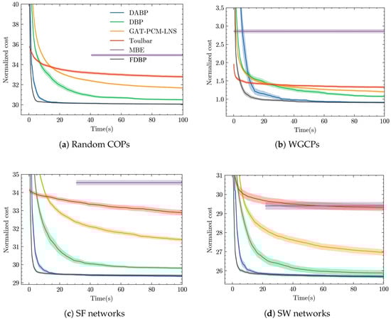
Figure 2. Solution quality versus time. Shaded regions depict 95% confidence intervals. Note that MBE is an elimination-based approximator: it first selects an elimination ordering and performs mini-bucket partitioning, then executes a backward elimination pass to compute bounds/messages, and finally runs a forward decoding pass to reconstruct a concrete assignment. A valid objective is available only after this decode step, so the cost–time curve for MBE starts once the first assignment is produced.

• FDBP consistently outperforms all other methods across all problem types, demonstrating the fastest convergence to the optimal or near-optimal solution with the lowest normalized cost. This suggests that FDBP is the most efficient algorithm overall.
• DABP and DBP generally show slower but steady improvement, with DABP typically outperforming DBP.
• GAT-PCM-LNS and Toulbar show slower progress and are less effective in terms of both speed and quality of the solution compared to FDBP, DABP, and DBP.
• MBE consistently reaches a plateau early but at a much higher cost than the other methods, indicating that while it converges faster, it is less effective at finding low-cost solutions.

Overall, the figures highlight the superiority of FDBP in terms of both speed and the quality of the solution across all problem instances. The other algorithms, while effective to some extent, generally converge slower and achieve higher costs, with MBE being the least competitive in terms of performance.

Albation Study. In loopy BP, messages at step t summarize the influence of steps $0,\dots ,t-1$. Conditioning the inference network for restart r on ${\left(m_{x\to f}^{t-1},m_{f\to x}^{t-1}\right)}^{r-1}$, therefore, provides near-sufficient context for predicting ${\lambda }^t$ and $w^t$ without constructing an intra-iteration autoregressive encoder. This preserves standard BP updates while avoiding sequential neural calls, reducing latency and memory. To confirm this, we also implemented an intra-iteration variant (FDBP-AR). On $\left|X\right|\in \{80,100\}$, FDBP-AR attains similar cost/gap but requires $\approx 2\times$ runtime and 15–$25\%$ higher peak GPU memory (see Table 3).

Table 3. Comparison of FDBP and FDBP-AR on random COPs ($\left|X\right|=100$, $R=10$, $K=20$). FDBP: cost $32.05$, gap $0.14\%$, time 108 s, peak $6.3$ GB. FDBP-AR: cost $32.03$, gap $0.08\%$, time 235 s, peak $7.6$ GB. Similar trends are observed at $\left|X\right|=80$.

Method	Cost	Gap (%)	Time (s)	Peak GPU (GB)
FDBP	32.05	0.14	108	6.3
FDBP-AR	32.03	0.08	235	7.6

Sensitivity Analysis. We add a sensitivity study (Table 4). For the update interval K on $\left|X\right|=100$ with $R=10$, we observe a clear accuracy–efficiency trade-off—$K=5$ yields cost $32.02$, gap $0.06\%$, and 160 s; $K=10$ yields $32.04$, $0.10\%$, and 121 s; $K=20$ yields $32.05$, $0.14\%$, and 108 s; $K=40$ yields $32.13$, $0.37\%$, and 83 s—suggesting $K=20$ as a good balance. For damping, the range $[0.8,1.0]$ is stable and fast, whereas $[0.7,1.0]$ occasionally oscillates on WGCPs. For restarts, returns diminish beyond $R=20$; for $\left|X\right|=100$, increasing from $R=10$ to $R=20$ increases time from 108 s to 222 s for only a $0.11\%$ gap improvement. Finally, for GAT capacity, a smaller configuration $2\times 4\times 8$ is $14\%$ faster but slightly less accurate, a larger configuration $6\times 8\times 16$ is $38\%$ slower but slightly more accurate, and the default $4\times 4\times 8$ provides the best accuracy–efficiency balance.

Table 4. Sensitivity summary on random COPs ($\left|X\right|=100$, $R=10$).

Setting	Cost	Gap (%)	Time (s)	Peak GPU (GB)
$K=10$	32.04	0.10	121	6.2
$K=20$	32.05	0.14	108	6.1
Damping $[0.8,1.0]$	32.05	0.14	108	6.1
Damping $[0.7,1.0]$	32.09	0.28	109	6.2
GAT $2\times 4\times 8$	32.12	0.25	93	5.9
GAT $6\times 8\times 16$	32.01	0.09	149	6.6

6. Conclusions

This work addresses critical limitations in modern BP methods for COPs. While DBP improved convergence through manual damping heuristics, and DABP automated these via deep learning, both suffered from fundamental bottlenecks: DABP’s reliance on sequential RNNs for damping prediction introduced prohibitive memory overheads and limited scalability, while DBP’s manual tuning proved impractical for large-scale applications. We propose FDBP, a scalable BP framework that fundamentally rethinks how damping factors are learned. By decoupling damping inference from BP iterations and replacing RNNs with periodic message aggregation (every K steps), FDBP achieves the following:

• Memory Efficiency: Eliminates RNN hidden state storage, significantly reducing GPU memory usage compared to DABP, allowing scalability to 300-variable COPs, where DABP fails due to OOM issues.
• Computational Efficiency: Parallelizable message processing reduces runtime by an average of 65% at equivalent restart counts $\left(R\right)$, solving 100-variable COPs in 3m42s compared to DABP’s 5m44s, with only a 0.03% loss in solution quality.
• Practical Optimality: Maintains near-DABP performance (0.00–0.35% gaps) on small instances while outperforming all baselines on large-scale problems (e.g., 300-variable WGCPs: 4.80 normalized cost vs DBP’s 5.24).

Empirical results across synthetic and topology-driven benchmarks confirm that FDBP’s design choices successfully balance the accuracy–efficiency tradeoff.

Limitations and future work. This work focuses on static, single-agent COPs; time-varying structures and decentralized coordination are out of scope. In future work, we will extend the framework to dynamic COPs and multi-agent systems by adding online message updates, warm starts, and communication-efficient, decentralized controllers, enabling more adaptive and distributed problem solving.

Broader implications. This work advances applied mathematics, computing, and machine learning by coupling model-based belief propagation with a lightweight learned controller, which preserves interpretability while improving efficiency. The framework is GPU-friendly and memory-efficient, aligning with high-performance computing for AI. It supports uncertainty-aware decisions via belief estimates and applies broadly to discrete-optimization tasks in science and engineering, including scheduling, routing, network design, and error-correcting codes. This strengthens applied machine learning and AI for scientific discovery under fixed hardware budgets.

References

- Pearl, J. Probabilistic Reasoning in Intelligent Systems: Networks of Plausible Inference; Morgan Kaufmann: Burlington, MA, USA, 1988. [Google Scholar]
- Kschischang, F.R.; Frey, B.J.; Loeliger, H.A. Factor graphs and the sum-product algorithm. IEEE Trans. Inf. Theory 2001, 47, 498–519. [Google Scholar] [CrossRef]
- Yedidia, J.S.; Freeman, W.T.; Weiss, Y. Constructing free-energy approximations and generalized belief propagation algorithms. IEEE Trans. Inf. Theory 2005, 51, 2282–2312. [Google Scholar] [CrossRef]
- Aji, S.M.; McEliece, R.J. The generalized distributive law. IEEE Trans. Inf. Theory 2000, 46, 325–343. [Google Scholar] [CrossRef]
- MacKay, D.J. Information theory, Inference and Learning Algorithms; Cambridge University Press: Cambridge, UK, 2003. [Google Scholar]
- Modi, P.J.; Shen, W.M.; Tambe, M.; Yokoo, M. ADOPT: Asynchronous distributed constraint optimization with quality guarantees. Artif. Intell. 2005, 161, 149–180. [Google Scholar] [CrossRef]
- Rossi, F.; van Beek, P.; Walsh, T. Handbook of Constraint Programming; Elsevier Science Inc.: Amsterdam, The Netherlands, 2006. [Google Scholar]
- Kong, S.; Lee, J.H.; Li, S. A deterministic distributed algorithm for reasoning with connected row-convex constraints. In Proceedings of the 16th Conference on Autonomous Agents and MultiAgent Systems, São Paulo, Brazil, 8–12 May 2017; pp. 203–211. [Google Scholar]
- Kong, S.; Lee, J.H.; Li, S. Multiagent simple temporal problem: The Arc-consistency approach. In Proceedings of the AAAI Conference on Artificial Intelligence, New Orleans, LA, USA, 2–7 February 2018. [Google Scholar]
- Bertsekas, D.P. Constrained Optimization and Lagrange Multiplier Methods; Academic Press: New York, NY, USA, 2014. [Google Scholar]
- Farinelli, A.; Rogers, A.; Petcu, A.; Jennings, N.R. Decentralised coordination of low-power embedded devices using the Max-sum algorithm. In Proceedings of the AAMAS, Estoril, Portugal, 3–7 May 2008; pp. 639–646. [Google Scholar]
- Wainwright, M.J.; Jaakkola, T.S.; Willsky, A.S. Tree-reweighted belief propagation algorithms and approximate ML estimation by pseudo-moment matching. In Proceedings of the AISTATS, Key West, FL, USA, 3–6 January 2003. [Google Scholar]
- Globerson, A.; Jaakkola, T. Fixing max-product: Convergent message passing algorithms for MAP LP-relaxations. In Proceedings of the NeurIPS, Vancouver, BC, Canada, 3–6 December 2007. [Google Scholar]
- Dechter, R. Bucket elimination: A unifying framework for reasoning. Artif. Intell. 1999, 113, 41–85. [Google Scholar] [CrossRef]
- Dechter, R.; Rish, I. Mini-buckets: A general scheme for bounded inference. J. ACM 2003, 50, 107–153. [Google Scholar] [CrossRef]
- Rogers, A.; Farinelli, A.; Stranders, R.; Jennings, N.R. Bounded approximate decentralised coordination via the max-sum algorithm. Artif. Intell. 2011, 175, 730–759. [Google Scholar] [CrossRef]
- Rollon, E.; Larrosa, J. Improved bounded max-sum for distributed constraint optimization. In Proceedings of the International Conference on Principles and Practice of Constraint Programming, Québec City, QC, Canada, 8–12 October 2012; pp. 624–632. [Google Scholar]
- Rollon, E.; Larrosa, J. Decomposing utility functions in bounded max-sum for distributed constraint optimization. In Proceedings of the International Conference on Principles and Practice of Constraint Programming, Lyon, France, 8–12 September 2014; Springer International Publishing: Cham, Switzerland, 2014; pp. 646–654. [Google Scholar]
- Chen, Z.; Deng, Y.; Wu, T.; He, Z. A class of iterative refined Max-sum algorithms via non-consecutive value propagation strategies. Auton. Agents Multi-Agent Syst. 2018, 32, 822–860. [Google Scholar] [CrossRef]
- Zivan, R.; Parash, T.; Cohen, L.; Peled, H.; Okamoto, S. Balancing exploration and exploitation in incomplete min/max-sum inference for distributed constraint optimization. Auton. Agents Multi-Agent Syst. 2017, 31, 1165–1207. [Google Scholar] [CrossRef]
- Cohen, A.; Galiki, R.; Meisels, A.; Grunitzki, R.; Zivan, R. Governing convergence of Max-sum on DCOPs through damping and splitting. Artif. Intell. 2020, 279, 103212. [Google Scholar] [CrossRef]
- Kuck, J.; Chakraborty, S.; Tang, H.; Luo, R.; Song, J.; Sabharwal, A.; Ermon, S. Belief Propagation Neural Networks. Adv. Neural Inf. Process. Syst. 2020, 33, 667–678. [Google Scholar]
- García Satorras, V.; Hoogeboom, E.; Welling, M. Neural Enhanced Belief Propagation on Factor Graphs. In Proceedings of the International Conference on Artificial Intelligence and Statistics, Valencia, Spain, 13–15 April 2021. [Google Scholar]
- Zhang, Z.; Dupty, M.H.; Wu, F.; Shi, J.Q.; Lee, W.S. Factor Graph Neural Networks. J. Mach. Learn. Res. 2023, 24, 1–54. [Google Scholar]
- Cappart, Q.; Chételat, D.; Khalil, E.B.; Lodi, A.; Morris, C.; Veličković, P. Combinatorial Optimization and Reasoning with Graph Neural Networks. J. Mach. Learn. Res. 2023, 24, 1–61. [Google Scholar]
- Sun, Y.; Yang, Q. DIFUSCO: Graph-Based Diffusion Solvers for Combinatorial Optimization. Adv. Neural Inf. Process. Syst. 2023, 36, 3706–3731. [Google Scholar]
- Li, Y.; Guo, J.; Wang, R.; Zha, H.; Yan, J. Fast T2T: Consistency Models for Faster Discrete Combinatorial Optimization. Adv. Neural Inf. Process. Syst. 2024, 37, 30179–30206. [Google Scholar]
- Yu, J.; Han, Y.; Xu, M.; Chen, S.; Gu, S. DISCO: Diffusion for Large-Scale Combinatorial Optimization. arXiv 2024, arXiv:2406.19705. [Google Scholar]
- Zhang, X.; Chen, Z.; Cai, S. Revisiting Restarts of CDCL: Should the Search Information be Preserved? arXiv 2024, arXiv:2404.16387. [Google Scholar] [CrossRef]
- Li, C.; Liu, C.; Chung, J.; Lu, Z.; Jha, P.; Ganesh, V. A Reinforcement Learning Based Reset Policy for CDCL SAT Solvers. arXiv 2024, arXiv:2404.03753. [Google Scholar] [CrossRef]
- Yau, M.; Karalias, N.; Lu, E.; Xu, J.; Jegelka, S. Are Graph Neural Networks Optimal Approximation Algorithms? Adv. Neural Inf. Process. Syst. 2024, 37, 73124–73181. [Google Scholar]
- Lawler, E.L.; Wood, D.E. Branch-and-bound methods: A survey. Oper. Res. 1966, 14, 699–719. [Google Scholar] [CrossRef]
- Deng, Y.; Kong, S.; Liu, C.; An, B. Deep Attentive Belief Propagation: Integrating Reasoning and Learning for Solving Constraint Optimization Problems. In Proceedings of the NeurIPS, New Orleans, LA, USA, 28 November–9 December 2022. [Google Scholar]
- Gomes, C.P.; Selman, B.; Kautz, H. Boosting combinatorial search through randomization. In Proceedings of the Fifteenth National/Tenth Conference on Artificial Intelligence/Innovative Applications of Artificial Intelligence, Madison, WI, USA, 27 July 1998; pp. 431–437. [Google Scholar]
Disclaimer/Publisher’s Note: The statements, opinions and data contained in all publications are solely those of the individual author(s) and contributor(s) and not of MDPI and/or the editor(s). MDPI and/or the editor(s) disclaim responsibility for any injury to people or property resulting from any ideas, methods, instructions or products referred to in the content. |
© 2025 by the authors. Licensee MDPI, Basel, Switzerland. This article is an open access article distributed under the terms and conditions of the Creative Commons Attribution (CC BY) license (https://creativecommons.org/licenses/by/4.0/).