EmbTCN-Transformer: An Embedding Temporal Convolutional Network–Transformer Model for Multi-Trajectory Prediction

Abstract

This paper addresses the multi-trajectory prediction problem and a so-called Embedded-TCN-Transformer (EmbTCN-Transformer) model is designed by using the real-time historical trajectories in a formation. A temporal convolutional network (TCN) is utilized as the input embedding to introduce temporal awareness capabilities into the model. Then, the self-attention mechanism is incorporated as the backbone to extract correlations among different positions of the trajectory. An encoder–decoder structure is adopted to generate future trajectories. Ablation experiments validate the effectiveness of the EmbTCN-Transformer, showing that the TCN-based input embedding and the self-attention mechanism contribute to 30% and 80% reductions in prediction error, respectively. Comparative experiments further demonstrate the superiority of the proposed model, achieving at least 60% and 10% performance improvements over Recurrent Neural Network (RNN)-based networks and the conventional Transformer, respectively.

1. Introduction

Nowadays, trajectory prediction is a hot topic due to its applications in various scenarios, e.g., autonomous driving [1,2], maritime transportation [3], traffic management [4] and target tracking [5,6]. Various methods have been proposed in this field including Kalman filters [7], particle filters [8] and neural networks [9,10,11,12,13,14,15,16,17]. An Extended Kalman Filter (EKF) is used in [7] for a drone to achieve a spatial position estimation of moving targets. A particle filtering algorithm is designed in [8] to solve the filtering equation in multi-aircraft trajectory prediction. However, the above trajectory prediction algorithms rely on prior models and expert experience. Therefore, it is a trend to extract deep-seated features from historical trajectories and hence the constrained accuracy in traditional trajectory prediction can be solved.

Due to its strong learning capability, generalization ability and portability, deep learning has been widely applied in trajectory prediction. In [9], RNNs are used to predict the moving information based on sequential and time-series data. In [10], convolutional layers are embedded into Long Short-Term Memory (LSTM) to predict flight trajectories based on convective weather conditions and flight plans before aircraft takeoff. A similar trajectory prediction model is given in [11] by introducing a sliding window in LSTM, which maintains the continuity of trajectory prediction and at the same time avoids the dynamic dependencies between neighboring states in long-term sequences. An innovative online learning model is integrated into k-means clustering and a Gated Recurrent Unit (GRU) in [12] to adaptively cluster aircraft trajectory points and then employ an online learning prediction.

However, RNN-based networks have weaker capabilities in handling long sequences. As the sequence length increases, the temporal features of RNN-based networks will be diluted and hence lead to a decreased ability to extract features. To this end, attention-based networks and Transformers are introduced to operate trajectory predictions. An Attention-based Convolutional Long Short-Term Memory (AttConvLSTM) network is designed in [13] to calculate the arrival probabilities of various spatial locations within the reachable area of a target aircraft. By segmenting the reachable area and transforming the trajectory prediction challenge into a classification problem, this network can reach the optimal solution. The Transformer network is introduced into the trajectory prediction task in [14] and demonstrates the superiority of self-attention-based networks. The Transformer network can effectively capture the interdependencies among different positions within a trajectory sequence. Building on this, a BERT network is further developed in [15] for trajectory prediction. In [16], a Transformer model is designed for accurate vessel trajectory prediction within maritime traffic, where its decoder consists of fully connected layers based on the abundant vessel trajectory data from the Automatic Identification System (AIS) and the encoder–decoder architecture of the Transformer model. To tackle the inherent complexity and multimodality of motion data in AIS, the TrAISformer model is proposed in [17], an improved Transformer network that can extract long-term correlations of AIS trajectories in a proposed enriched space to predict the future positions of vessels within the next few hours. It is noted that the above approaches indicate the superiority of the model through attention mechanisms. However, incorporating attention mechanisms into traditional RNN-based networks alone does not enable parallel computation, which may increase the training time. Note that the Transformer network is solely based on self-attention mechanisms to extract positional relationship features from sequences. There is still some loss of temporal information regarding the relationship between different positions in a time sequence despite the addition of positional encoding.

Owing to the strong capability of convolutional networks in temporal awareness [18] and the superior ability of self-attention mechanisms in capturing long-term dependencies and positional information, the two are often combined and applied in various domains, such as agriculture [19], medicine [20] and time-series classification [21]. Integrating convolutional networks into self-attention-based models can effectively enhance their sensitivity to temporal features, thereby compensating for the tendency of self-attention networks to emphasize positional information while overlooking temporal information.

Based on the above discussion, this paper designs a novel model, that is, the EmbTCN-Transformer, to capture long-term dependencies in sequential trajectory data. To incorporate additional information about the relationship between different positions in the time series, the fully connected input embedding module in the Transformer network is replaced by the TCN [18], transforming a simple linear mapping into the capability of perceiving information within trajectory segments. As a result, the efficiency of trajectory prediction is enhanced effectively as compared to LSTM, GRU and Transformer architectures.

The paper is organized as follows. Section 2 is the problem statement of trajectory prediction. The proposed EmbTCN-Transformer model is illustrated in Section 3. Section 4 provides the simulation results. Conclusions and future work are provided in Section 5.

2. Problem Statement

In this work, the trajectory prediction problem is formulated as a neural network fitting an output sequence based on a given input sequence. Let ${\mathit{x}}_t^i$ be the positional information of the target i at time t, that is,

$${\mathit{x}}_t^i=\left(x_t^i,y_t^i,z_t^i\right),$$

(1)

where $x_t^i$ and $y_t^i$ are horizontal and vertical coordinates of UAV i in regional tactical map. $z_t^i$ is the height of UAV i. The true historical trajectory data of the target i is

$${\mathit{X}}^i=\left\{{\mathit{x}}_1^i,{\mathit{x}}_2^i,\dots ,{\mathit{x}}_m^i\right\},$$

(2)

where ${\mathit{X}}_t^i$ is the historical trajectory data; m is the length of the historical trajectory. The trajectory prediction process can be given by

$${\widehat{\mathit{Y}}}^i=F\left({\mathit{X}}_t^i\right),$$

(3)

where $F\left({\mathit{X}}_t^i\right)$ is the neural network model for trajectory prediction; ${\widehat{\mathit{Y}}}_t^i$ is the predicted trajectory whose ground truth is

$${\mathit{Y}}^i=\left\{{\mathit{y}}_1^i,{\mathit{y}}_2^i,\dots ,{\mathit{y}}_n^i\right\},$$

(4)

where n is the length of the predicted trajectory. Then, the destination of this work can be transformed into minimizing the error of ${\widehat{\mathit{Y}}}_t^i$ and ${\mathit{Y}}_t^i$. The error e can be calculated by

$$e={\displaystyle \frac{1}{l}}{\displaystyle \sum _i^l{‖{\widehat{\mathit{Y}}}^i-{\mathit{Y}}^i‖}_2}$$

(5)

where l is the number of the target; ${‖\cdot ‖}_2$ indicates the 2-norm.

3. Methodology

In this paper, a so-called EmbTCN-Transformer model is proposed to predict the multi-trajectory path. Its structure is shown in Figure 1, which consists of a TCN input embedding module (Section 3.1), encoder (Section 3.2), decoder (Section 3.3) and others of the network (Section 3.4).

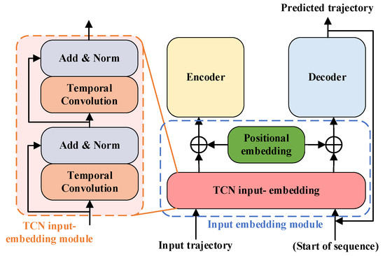
Figure 1. The structure of EmbTCN-Transformer model.

3.1. TCN Input Embedding Module

The embedding module is positioned before the encoder and decoder and is utilized to transform input sequences into vectors that are more manageable for the encoder and decoder. The embedding layer in the Transformer standardizes the input temporal series of varying lengths into fixed-length embedding vectors. Additionally, positional information is embedded through a positional encoding layer. In contrast to the linear layers used in a traditional Transformer [22], the input embedding layer in EmbTCN-Transformer employs a TCN network.

TCN is a neural network that utilizes a 1D fully convolutional network to address sequence-to-sequence problems. TCN can handle tasks involving sequences of arbitrary length while enabling parallel processing and flexible adjustment of receptive field size. The structure of TCN is illustrated in Figure 1. A temporal convolution block in TCN consists of causal convolution and dilated convolution. To put it simply, TCN can be defined as

$$\mathrm{TCN}=1\mathrm{D} \mathrm{FCN}+\mathrm{Causal} \mathrm{Conv}+\mathrm{Dilated} \mathrm{Conv}$$

(6)

where the $1\mathrm{D} \mathrm{FCN}$ refers to one-dimension fully convolution network; Causal Conv refers to causal convolution, that is, the value of the current time step in the convolutional layer depends only on the values at the current time step and earlier in the previous layer. It ensures no leakage of future information in the sequence. Dilated Conv refers to dilated convolution, where holes are introduced in the convolutional kernel to address the issue of increased computation in causal convolution when dealing with variable-length sequences, and it also increases the receptive field. The process of causal convolution and dilated convolution is represented in Figure 2 and Figure 3.

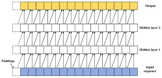
Figure 2. Causal convolutions.

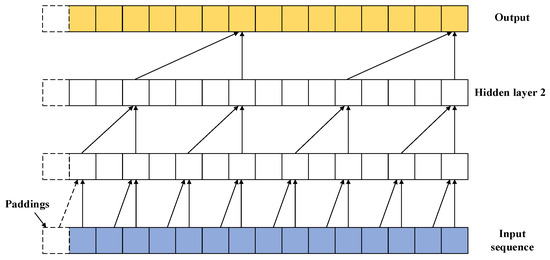
Figure 3. Causal convolutions with dilated convolutions.

In the EmbTCN-Transformer, TCN introduces temporal awareness into the embedded tensor, a perceptual ability absent in the original Transformer’s linear embedding layer. The input of the EmbTCN-Transformer contains both temporal and sequential correlations among the trajectory, rather than the linear mapping of positional features only in conventional Transformer networks. The temporal features extracted by TCN compensate for the deficiency in the original Transformer by solely using positional embedding. The process can be given by

$$\left\{\begin{array}{l}{e}_t^i=TCN\left(I_t^i\right)+p_t^i\\ d_t^i=TCN\left({\widehat{I}}_t^i\right)+p_t^i\end{array}\right.$$

(7)

where $e_t^i$ is the encoder embedding tensors, $d_t^i$ is the decoder embedding tensors and $p_t^i$ is the positional encoding added to tensors. The encoder and decoder share the same weight matrix in the embedding process.

3.2. Encoder

The encoder is EmbTCN-Transformer consists of 4 identical layers, which contains a multi-head self-attention sub-layer and a fully connected feed-forward sub-layer [14]. The multi-head self-attention mechanism converts the positional relationships between input sequences into mathematical expectations through scoring, that is,

$$\begin{array}{l} \\ Attention(Q,K,V) =SoftMax\left({\displaystyle \frac{Q{K}^T}{\sqrt{d_k}}}\right)V\end{array}$$

(8)

where Q, K and V are Query, Key and Value vectors, respectively, and they are obtained by

$$\begin{array}{l} \\ \left\{\begin{array}{l}Q=W^Q{e}_t^i\\ K=W^K{e}_t^i\\ V=W^V{e}_t^i\end{array}\right.\end{array}$$

(9)

where WQ, WK and WV are weight matrices for Query, Key and Value. The multi-head attention mechanism consists of multiple heads, where multiple sets of attention are concatenated and weighted, each focusing on different positions in the sequence. The process is shown in Figure 4. In EmbTCN-Transformer, there are 8 heads.

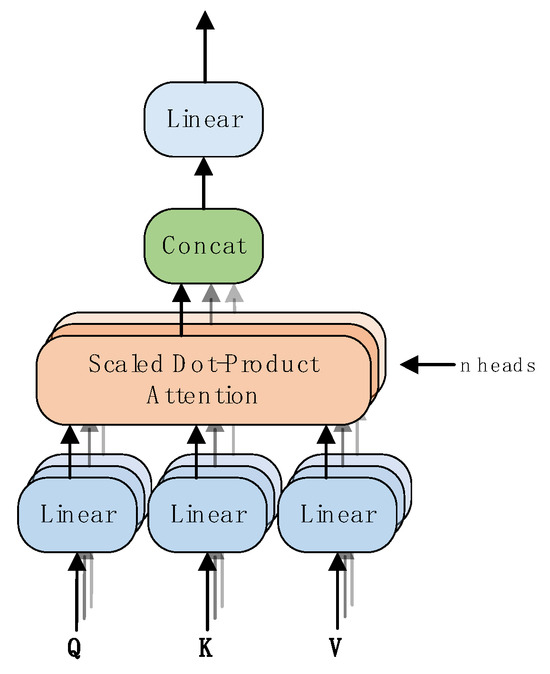
Figure 4. Multi-head self-attention mechanism.

The output of the encoder is a “memory” and is used in decoder layers as Key and Value vectors, which is represented as:

$$m^i=Encoder\left(e_t^i,n_{sub},n_{head}\right)$$

(10)

where mi is the “memory”, n_sub is the number of sub-layers and n_head is the number of heads.

3.3. Decoder

In the EmbTCN-Transformer, the layers of the decoder and encoder are consistent. Compared with encoder layers, an encoder–decoder attention sub-layer is inserted between the self-attention module and the feed-forward module, which utilizes “memory”, the encoder output, as Key and Value and Query vectors from the preceding multi-head self-attention sub-layer. The decoder takes the previous step prediction result and “memory” as input, producing the prediction for the next step in the output sequence. This process repeats until a sequence of the desired length is generated. For the training process, the input sequence of decoder is ground truth with masks to avoid leaking future values. The process of the decoder are

$${\widehat{I}}_t^i=Decoder\left(d_t^i,m^i,n_{sub},n_{head}\right)$$

(11)

where $n_{sub}$ is the number of sub-layers and $n_{head}$ is the number of heads.

3.4. Complexity Analysis

The TCN is a one-dimensional convolutional neural network with a time complexity of $O\left(C_{in}{C}_{out}Kn\right)$, where $C_{in}$ denotes the input dimension, $C_{out}$ the output dimension, $K$ the convolution kernel size and $n$ the aforementioned input trajectory length. Correspondingly, its space complexity is $O\left(C_{in}{C}_{out}K\right)$. For a linear layer network, its time complexity is $O\left(C_{in}{C}_{out}\right)$, indicating that $C_{in}$ and $C_{out}$ are primary determining factor for time consumption. Similarly, the space complexity is also $O\left(C_{in}{C}_{out}\right)$.

Since $K$ is typically small and constant, and $n$ is also constant, while $C_{in}$ is usually 2 or 3 as the input embedding dimension for trajectory prediction, the dominant term in the complexity of both networks is $C_{out}$. Therefore, the complexity of the TCN does not increase significantly compared to the linear layer. Moreover, unlike the linear layer, computations across different channels in the TCN can be parallelized, leading to reduced time consumption in practical training and inference.

3.5. Others

Pairwise distance is selected as the loss function to evaluate the error between the predicted trajectory and ground truth. The network is trained via backpropagation using the Adam optimizer with a linear warm-up phase for the first 10 epochs. The loss function is given by

$$Loss={\displaystyle \frac{1}{NT}}{\displaystyle \sum _{i=0}^n{\displaystyle \sum _{t=0}^T\sqrt{{\left({\widehat{x}}_t^i-x_t^i\right)}^2+{\left({\widehat{y}}_t^i-y_t^i\right)}^2+{\left({\widehat{z}}_t^i-z_t^i\right)}^2}}}$$

(12)

where N is the batch size and T is the length of a sequence.

4. Experiment Results

In this section, parameter selection experiments are conducted to identify the model parameters that yield the optimal results on the test set. Comparative analyses with LSTM, GRU and traditional Transformer networks demonstrate the superiority of our EmbTCN-Transformer network. Additionally, ablation experiments were performed to illustrate the effectiveness of the model improvements. All models in this chapter were trained for 200 epochs with a batch size of 100.

4.1. Experiment Settings

The deep learning framework is PyTorch 1.12.1 and programming language Python 3.10 in on an x86-64 Ubuntu-20.04 PC based on Intel^® Xeon(R) Silver 4110 CPU @ 2.10 GHz, 128 GB RAM and NVIDIA^® GeForce RTX 3080Ti GPU with CUDA 12.2 (Supermicro, Shanghai, China) to accelerate computation.

4.2. Dataset

The dataset is generated by a rotary-wing UAV formation simulation engine. During operation, the engine can configure one or more UAV formations to fly within a designated area according to predefined rules. The engine provides a simplified simulation of UAV aerodynamics and outputs the position state of each UAV at a frequency of one sample per second. Through multiple simulations, All UAVs’ trajectories are obtained, curated and filtered across 65,000 flight trajectory samples. Each sample involves continuous information collected over 20 frames, with each frame comprising three dimensions, including UAVs’ coordinates on the tactical map, and the altitude. The coordinates and altitude data are used to train and predict the trajectory. The first 10 frames contain historical trajectory data, and the subsequent 10 frames are the ground truth. The proportions of the training set, validation set and test set are 88%, 5% and 7%, respectively, amounting to 76,700 training data samples, 3750 validation data samples and 4550 test data samples.

To enhance prediction performance, the input position sequences are converted into velocity sequences by subtracting the previous position from the current one in the sequences. Subsequently, the training data are normalized to the [0, 1] range by subtracting the mean and dividing by the standard deviation of the training data [14].

4.3. Metrics

The evaluation metrics employed are commonly used in the literature on human trajectory prediction. The network performance is assessed using two metrics: Average Displacement Error (ADE), which is the L2 average distance between the true and predicted trajectories, and Final Displacement Error (FDE), which is the L2 distance between the predicted final position and the true final position [23]. The average values of ADE and FDE are used to evaluate the performance of each network, where lower values for ADE and FDE indicate better performance. The equations for ADE and FDE processing a single trajectory prediction of a certain UAV i are given by

$$AD{E}_i={\displaystyle \frac{1}{t}}{\displaystyle \sum _{t=0}^T\sqrt{{\left({\widehat{x}}_t^i-x_t^i\right)}^2+{\left({\widehat{y}}_t^i-y_t^i\right)}^2+{\left({\widehat{z}}_t^i-z_t^i\right)}^2}}$$

(13)

$$\begin{array}{l} \\ FD{E}_i={\displaystyle \frac{1}{t}}\sqrt{{\left({\widehat{x}}_T^i-x_T^i\right)}^2+{\left({\widehat{y}}_T^i-y_T^i\right)}^2+{\left({\widehat{z}}_T^i-z_T^i\right)}^2}\end{array}$$

(14)

4.4. Parameter Selection Experiments

In the experiment, hyperparameters are adjusted to optimize the performance of the EmbTCN-Transformer network. The parameters of the original Transformer model are adopted as the initial parameters for the Transformer part, i.e., $d_{model}=512$, six layers of encoder and decoder and eight attention heads. The initial parameters for the TCN network in the input embedding layer are three layers of TCN network with 60 hidden units per layer with kernel size of five. The dropout rate of the network is 0.1.

Based on this, the parameters that need to be adjusted contains the number of layers in the TCN network, the hidden units in the TCN network and the convolutional kernel size of the TCN. (1) The number of hidden units in the TCN network is set to n_dim = 50, 60, 70, 80, 90, 100, and the optimal number is determined, as shown in Figure 5a; (2) based on the results of (1), set tcn_layers = 2, 3, 4, 5, as shown in Figure 5b; (3) building on the results of (2), set the TCN network’s convolutional kernel to k_size = 4, 5, 6, 7, as shown in Figure 5c; (4) building on the results of (3), set numbers of layers in the encoder and decoder to n_layers = 3, 4, 5, 6, 7, as shown in Figure 5d.

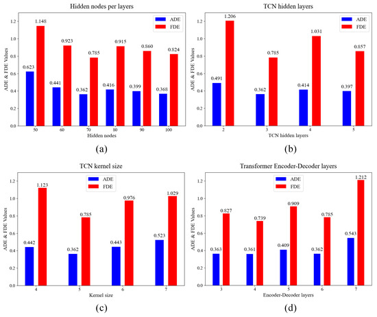
Figure 5. Parameter selection experiments. (a) Influence of the number of hidden nodes per TCN layers on model performance; (b) influence of the number of hidden layers of TCN on model performance; (c) influence of number of TCN kernel size on model performance; (d) influence of number of Transformer encoder–decoder layers on model performance.

From Figure 5a, it is evident that as the number of nodes per hidden layer in the TCN increases, both ADE and FDE decrease and reach their minimum when the number of hidden nodes per layer arrives 70. However, further increases in hidden nodes result in overfitting, particularly in the FDE metric. Set the number of hidden nodes to 100. Although the difference in ADE compared to when there are 70 hidden nodes is minimal (less than 1%), there is still a significant gap in the FDE metric. Figure 5b demonstrates that a moderate increase in the number of hidden layers in the TCN contributes to improved prediction accuracy, with the optimal performance achieved when the number of hidden layers is six. However, an excessive number of hidden layers leads to model overfitting, diminishing model stability. According to Figure 5c, the impact of the TCN’s convolutional kernel size on model performance is more pronounced. Both excessively large and small kernel sizes noticeably affect network performance, with the best results achieved when the kernel size is five. As depicted in Figure 5d, a single-layer encoder–decoder structure has a large parameter count, and variations in the number of layers in the encoder and decoder have the most significant impact on model performance among the four parameters. The optimal performance is achieved when the number of encoder and decoder layers is four. This is because, compared to the Transformer, whose number of encoder and decoder layers is six, the EmbTCN-Transformer replaces the linear layer in the input embedding with TCN, resulting in an increased parameter count. Reducing the number of encoder and decoder layers is necessary to avoid severe overfitting.

Based on the above experimental results, the EmbTCN-Transformer is configured with 70 hidden units in the TCN, three TCN hidden layers, a convolution kernel size of five and six layers in the encoder–decoder structure. The detailed parameter settings and other configurations are presented in Table 1. The number of heads and the embedding size follow the settings in [22].

Table 1. Parameters of EmbTCN-Transformer.

Parameter	Value
Input sequence length	10
Predicted sequence length	10
Number of heads	8
Embedding size	512
Number of encoder–decoder layers	6
Number of TCN layers	3
Number of hidden units per TCN layers	70
Batch size	100
Max epoch	200
Warm-up epoch	10
Dropout	0.1
Optimizer	Adam
Loss function	Pairwise distance

4.5. Result Analysis of EmbTCN-Transformer

The training of the EmbTCN-Transformer involves synchronous testing on the test set, with the training set loss values and test set ADE and FDE values shown in Figure 6a,b. Figure 7 presents the test results for two individual fighters, while Figure 8 shows the test results for a trapezoidal fighter formation.

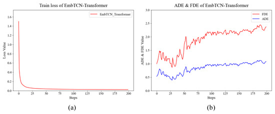
Figure 6. Results of EmbTCN-Transformer. (a) Training set loss values; (b) test set ADE and FDE values.

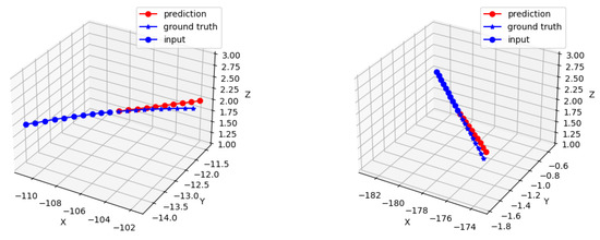
Figure 7. Test results for two individual UAVs.

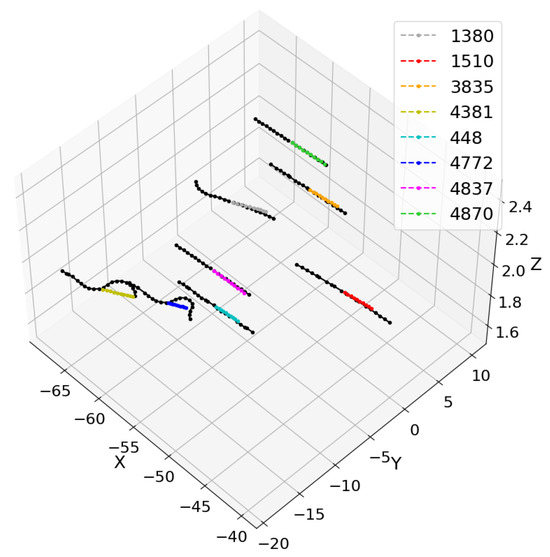
Figure 8. Test results for a trapezoidal UAV formation.

From Figure 6a, it is evident that after 200 training epochs, the model converges to a final loss of 0.02255. Overfitting begins around the 25th epoch, and the model achieves its best results on the test set around the 27th epoch, with an ADE of 0.3606 and an FDE of 0.7386. The training and test results for the EmbTCN-Transformer are summarized in Table 2.

Table 2. Results of EmbTCN-Transformer.

Training Loss	0.02255
Best result epoch	27
Best ADE	0.3606
Best FDE	0.7386

Figure 7 reveals that trajectory prediction aligns well with the overall direction and velocity forecasts of fighter UAV trajectories. Figure 8 depicts a forming trapezoidal fighter formation, with two UAVs in the front and five in the rear. The trajectory prediction is generally accurate for UAVs flying straight or engaged in minor maneuvering within the fighter formation. Notably, for the UAV number 1380, the trajectory prediction accurately maintains the direction and velocity after maneuvering. However, for UAV numbers 4381 and 4772, both are engaged in substantial maneuvers to adjust their positions and attitudes within the formation. The model can only predict a portion of their maneuvers or small-scale maneuvers, indicating a limitation in the overall predictive capability for extensive and comprehensive maneuvers.

4.6. Comparative Analysis of Trajectory Prediction Methods

This paper compares the EmbTCN-Transformer trajectory prediction model with baselines including LSTM [24], GRU and the original Transformer [22]. Comparative results are presented in Figure 9 and Table 3. GRU and LSTM both have four layers with 512 hidden units.

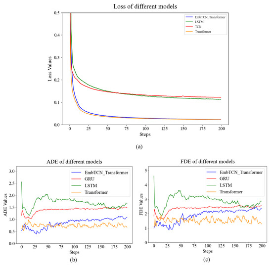
Figure 9. Experimental results of EmbTCN-Transformer and baselines. (a) Training loss of different models; (b) ADE of different models; (c) FDE of different models.

Table 3. Results of different models and relative improvement of EmbTCN-Transformer.

Model	ADE/Improvement	FDE/Improvement
LSTM	1.103/67%	1.725/57%
GRU	0.9877/63%	1.563/52%
Transformer	0.4096/12%	0.7815/5.5%
EmbTCN-Transformer	0.3606/-	0.7386/-

By comparing ADE and FDE metrics, it is evident that EmbTCN-Transformer outperforms all baseline models, exhibiting a 12%, 63% and 67% reduction in ADE and a 5.5%, 52% and 57% reduction in FDE compared to original Transformer, GRU and LSTM. Figure 10 illustrated that EmbTCN-Transformer outperforms all baselines to have the best performance in predicting the trajectory both in directions and velocities of UAVs.

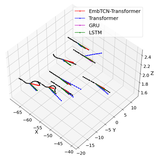
Figure 10. Experimental results of EmbTCN-Transformer and baselines predicting a trapezoidal UAV formation.

The results of LSTM and GRU are similar to each other, and Transformer exhibits instability in both direction and speed when predicting trajectories, indicating the non-negligible improvement from the involvement of long-range dependency perception ability. Meanwhile, EmbTCN-Transformer is the only model that accurately predicts directions of maneuvers from UAV number 4381 and 4772, demonstrating significantly better prediction performance than the conventional Transformer, both in quantitative evaluation metrics and in qualitative trajectory fitting. These results indicate that incorporating temporal awareness through the TCN embedding effectively enhances the model’s prediction capability, confirming the effectiveness and superiority of the proposed EmbTCN-Transformer network.

It is noteworthy that EmbTCN-Transformer is more susceptible to overfitting compared to other baseline models, leading to a gradual increase in ADE and FDE as the number of training epochs progresses. Moreover, compared with the Transformer, which converges around the 70th epoch, the EmbTCN-Transformer exhibits a faster convergence rate.

Overall, the EmbTCN-Transformer outperforms RNN-based networks such as LSTM and GRU in trajectory prediction, as well as the standard Transformer, demonstrating that integrating convolutional networks with self-attention mechanisms can effectively enhance prediction performance. This highlights the importance of incorporating temporal feature awareness into Transformer networks. Furthermore, owing to the parallel computation capability of convolutional networks and their faster convergence, the EmbTCN-Transformer achieves a balance between performance and computational cost among Transformer and RNN-based networks, delivering higher prediction accuracy without substantially increasing training and inference overhead.

4.7. Ablation Experiment

While the superiority of EmbTCN-Transformer has been demonstrated through comparisons with models such as LSTM, GRU and Transformer, it is important to note that they do not belong to the same network type. Moreover, the input embedding part of the proposed model has been modified compared with the conventional Transformer. Therefore, it is necessary to conduct ablation experiments to validate the effectiveness of our modifications.

The parameters of the EmbTCN-Transformer are the same as the models in the aforementioned sections and listed in Table 1. The baseline models consist of a TCN network, a Transformer network and a TCN-Transformer network. The TCN-Transformer network is a simple concatenation of both networks, while the input embedding of the latter part remains a conventional linear layer. The parameters of all baseline models are set to correspond closely to those of the proposed model. The experimental results are presented in Figure 11 and Table 4.

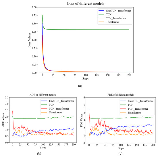
Figure 11. Results of ablation experiment. (a) Training loss of ablation experiment models; (b) ADE of ablation experiment models; (c) FDE of ablation experiment models.

Table 4. Results of ablation experiments.

Model Composition Structure		TCN Input Embedding	ADE	FDE
Transformer	TCN
√	√	√	0.3606	0.7386
	√		1.858	3.241
√			0.4727	0.8719
√	√		0.5173	1.015

From Table 4, it is evident that both metrics for EmbTCN-Transformer are lower than the other three models. Compared to TCN and Transformer, the EmbTCN-Transformer exhibits an 80%, 30% and 24% reduction in ADE, and a 77%, 27% and 15% reduction in FDE, respectively. Meanwhile, the EmbTCN-Transformer demonstrates a slightly improved performance compared with the TCN-Transformer, achieving a 24% reduction in ADE and a 15% reduction in FDE, indicating that the improvement achieved through our modifications cannot be realized by a simple concatenation of the two networks. This underscores the significant performance enhancement achieved by incorporating convolutional operations in the input embedding module, introducing information about different positions in the time series to the Transformer network.

It is worth noting that the performance of the four-layer encoder–decoder Transformer is inferior to the six-layer Transformer discussed in Section 4.6. This once again validates that replacing the fully connected network in the input embedding layer with TCN significantly increases the parameter count of the network. However, in TCN-Transformer, the parameter count becomes even higher than that of EmbTCN-Transformer due to the stacking of network structures, yet it does not yield better results. This demonstrates that blindly increasing the parameter count and network depth does not effectively enhance network performance.

5. Conclusions

This paper proposes the EmbTCN-Transformer model to solve UAV trajectory prediction in UAV formations. Replacing a fully connected input embedding module with TCN, the model gains temporal awareness capabilities and has been confirmed to outperform traditional trajectory prediction model in experiments.

However, the model exhibits limited predictive capability for extensive maneuvers of UAVs, and the variety of input sequence information is relatively limited. Investigating how to incorporate additional information and achieving trajectory predictions based on the intention recognition of the UAVs will be a focal point of our future research.

References

- Huang, Y.; Du, J.; Yang, Z.; Zhou, Z.; Zhang, L.; Chen, H. A survey on trajectory-prediction methods for autonomous driving. IEEE Trans. Intell. Veh. 2022, 7, 652–674. [Google Scholar] [CrossRef]
- Leon, F.; Gavrilescu, M. A review of tracking and trajectory prediction methods for autonomous driving. Mathematics 2021, 9, 660. [Google Scholar] [CrossRef]
- Zhang, X.; Fu, X.; Xiao, Z.; Xu, H.; Qin, Z. Vessel trajectory prediction in maritime transportation: Current approaches and beyond. IEEE Trans. Intell. Transp. Syst. 2022, 23, 19980–19998. [Google Scholar] [CrossRef]
- Schuster, W. Trajectory prediction for future air traffic management–complex manoeuvres and taxiing. Aeronaut. J. 2015, 119, 121–143. [Google Scholar] [CrossRef]
- Chong, C.-Y. An overview of machine learning methods for multiple target tracking. In Proceedings of the 2021 IEEE 24th International Conference On Information Fusion (FUSION), Sun City, South Africa, 1–4 November 2021; IEEE: Piscataway, NJ, USA, 2021. [Google Scholar] [CrossRef]
- Cao, X.; Ren, L.; Sun, C. Dynamic target tracking control of autonomous underwater vehicle based on trajectory prediction. IEEE Trans. Cybern. 2022, 53, 1968–1981. [Google Scholar] [CrossRef] [PubMed]
- Prevost, C.G.; Desbiens, A.; Gagnon, E. Extended Kalman filter for state estimation and trajectory prediction of a moving object detected by an unmanned aerial vehicle. In Proceedings of the 2007 American Control Conference, New York, NY, USA, 11–13 July 2007; IEEE: Piscataway, NJ, USA, 2007. [Google Scholar] [CrossRef]
- Lymperopoulos, I.; Lygeros, J. Sequential Monte Carlo methods for multi-aircraft trajectory prediction in air traffic management. Int. J. Adapt. Control Signal Process. 2010, 24, 830–849. [Google Scholar] [CrossRef]
- Salehinejad, H.; Sankar, S.; Barfett, J.; Colak, E.; Valaee, E. Recent advances in recurrent neural networks. arXiv 2017, arXiv:1801.01078. [Google Scholar] [CrossRef]
- Pang, Y.; Xu, N.; Liu, Y. Aircraft trajectory prediction using LSTM neural network with embedded convolutional layer. In Proceedings of the Annual Conference of the PHM Society, Scottsdale, AZ, USA, 23–26 September 2019; PHM Society: Bellevue, WA, USA, 2019; Volume 11. [Google Scholar] [CrossRef]
- Shi, Z.; Xu, M.; Pan, Q.; Yan, B.; Zhang, H. LSTM-based flight trajectory prediction. In Proceedings of the 2018 International Joint Conference on Neural Networks (IJCNN), Rio de Janeiro, Brazil, 8–13 July 2018; IEEE: Piscataway, NJ, USA, 2018. [Google Scholar] [CrossRef]
- Han, P.; Wang, W.; Shi, Q.; Yue, J. A combined online-learning model with K-means clustering and GRU neural networks for trajectory prediction. Ad Hoc Netw. 2021, 117, 102476. [Google Scholar] [CrossRef]
- Zhang, A.; Zhang, B.; Bi, W.; Mao, Z. Attention based trajectory prediction method under the air combat environment. Appl. Intell. 2022, 52, 17341–17355. [Google Scholar] [CrossRef]
- Giuliari, F.; Hasan, I.; Cristani, M.; Galasso, F. Transformer networks for trajectory forecasting. In Proceedings of the 2020 25th International Conference On Pattern Recognition (ICPR), Milan, Italy, 10–15 January 2021; IEEE: Piscataway, NJ, USA, 2021. [Google Scholar] [CrossRef]
- Franco, L.; Placidi, L.; Giuliari, F.; Hasan, I.; Cristani, M.; Galasso, F. Under the hood of transformer networks for trajectory forecasting. Pattern Recognit. 2023, 138, 109372. [Google Scholar] [CrossRef]
- Kang, K.; Zhang, C.; Guo, C. Ship trajectory prediction based on transformer model. In Proceedings of the 2022 4th International Conference on Data-Driven Optimization of Complex Systems (DOCS), Chengdu, China, 28–30 October 2022; IEEE: Piscataway, NJ, USA, 2022. [Google Scholar] [CrossRef]
- Nguyen, D.; Fablet, R. TrAISformer-A generative transformer for AIS trajectory prediction. arXiv 2021, arXiv:2109.03958. [Google Scholar] [CrossRef]
- Bai, S.; Kolter, J.Z.; Koltun, V. An empirical evaluation of generic convolutional and recurrent networks for sequence modeling. arXiv 2018, arXiv:1803.01271. [Google Scholar] [CrossRef]
- Osibo, B.K.; Ma, T.; Bediako-Kyeremeh, B.; Mamelona, L.; Darbinian, K. TCNT: A temporal convolutional network-transformer framework for advanced crop yield prediction. J. Appl. Remote Sens. 2024, 18, 044513. [Google Scholar] [CrossRef]
- Zheng, W.; Yan, L.; Wang, F.-Y. Two birds with one stone: Knowledge-embedded temporal convolutional transformer for depression detection and emotion recognition. IEEE Trans. Affect. Comput. 2023, 14, 2595–2613. [Google Scholar] [CrossRef]
- Chen, H.; Tian, A.; Zhang, Y.; Liu, Y. Early time series classification using TCN-transformer. In Proceedings of the 2022 IEEE 4th International Conference on Civil Aviation Safety and Information Technology (ICCASIT), Dali, China, 12–14 October 2022; IEEE: Piscataway, NJ, USA, 2022. [Google Scholar] [CrossRef]
- Vaswani, A.; Shazeer, N.; Parmar, N.; Uszkoreit, J.; Jones, L.; Gomez, A.N.; Kaiser, Ł.; Polosukhin, I. Attention is all you need. In Advances in Neural Information Processing Systems (NeurIPS) 30 (2017); NeurIPS: San Diego, CA, USA, 2017. [Google Scholar] [CrossRef]
- Zhu, Y.; Liu, J.; Guo, C.; Song, P.; Zhang, J.; Zhu, J. Prediction of battlefield target trajectory based on LSTM. In Proceedings of the 2020 IEEE 16th International Conference on Control & Automation (ICCA), Singapore, 9–11 October 2020; IEEE: Piscataway, NJ, USA, 2020. [Google Scholar] [CrossRef]
- Ivanovic, B.; Pavone, M. The trajectron: Probabilistic multi-agent trajectory modeling with dynamic spatiotemporal graphs. In Proceedings of the IEEE/CVF International Conference on Computer Vision, Seoul, Republic of Korea, 27 October–2 November 2019. [Google Scholar] [CrossRef]
Disclaimer/Publisher’s Note: The statements, opinions and data contained in all publications are solely those of the individual author(s) and contributor(s) and not of MDPI and/or the editor(s). MDPI and/or the editor(s) disclaim responsibility for any injury to people or property resulting from any ideas, methods, instructions or products referred to in the content. |
© 2025 by the authors. Licensee MDPI, Basel, Switzerland. This article is an open access article distributed under the terms and conditions of the Creative Commons Attribution (CC BY) license (https://creativecommons.org/licenses/by/4.0/).