Empirical Analysis of the Impact of Two Key Parameters of the Harmony Search Algorithm on Performance

Abstract

Metaheuristic algorithms are widely utilized as effective tools for solving complex optimization problems. Among them, the Harmony Search (HS) algorithm has garnered significant attention for its simple structure and excellent performance. The efficacy of the HS algorithm is heavily dependent on the configuration of its internal parameters, with the Harmony Memory Considering Rate (HMCR) and Pitch Adjusting Rate (PAR) playing pivotal roles. These parameters determine the probabilities of using the Random Generation (RG), Harmony Memory Consideration (HMC), and Pitch Adjustment (PA) operators, thereby controlling the balance between exploration and exploitation. However, a systematic empirical analysis of the interaction between these parameters and the characteristics of the problem at hand remains insufficient. Thus, this study conducts a comprehensive empirical analysis of the performance sensitivity of the HS algorithm to variations in HMCR and PAR values. The analysis is performed on a suite of 23 benchmark functions, encompassing diverse characteristics such as unimodality/multimodality and separability/non-separability, along with 5 real-world optimization problems. Through extensive experimentation, the performance for each parameter combination was evaluated on a rank-based system and visualized using heatmaps. The results experimentally demonstrate that the algorithm’s performance is most sensitive to the HMCR value across all function types, establishing that setting a high HMCR value (≥0.9) is a prerequisite for securing stable performance. Conversely, the optimal PAR value showed a direct correlation with the topographical features of the problem landscape. For unimodal problems, a low PAR value between 0.1 and 0.3 was more effective, whereas for complex multimodal problems with numerous local optima, a relatively higher PAR value between 0.3 and 0.5 proved more efficient in searching for the global optimum. This research provides a guideline into the parameter settings of the HS algorithm and contributes to enhancing its practical applicability by proposing a systematic parameter tuning strategy based on problem characteristics.

1. Introduction

The challenges encountered in numerous contemporary fields such as engineering, science, and management often manifest as complex and precise optimization problems that cannot be linearized. These problems may feature vast solution spaces, non-linearity, and numerous constraints, making it exceedingly difficult or impossible to find the optimal solution using traditional mathematical methodologies [1,2,3]. Consequently, metaheuristic algorithms, which draw inspiration from natural phenomena or mimic the behavioral patterns and strategies of animal or human, have emerged as a potent alternative [4]. Various metaheuristic techniques have been proposed, including the Genetic Algorithm, Particle Swarm Optimization, and Simulated Annealing. Among them, the Harmony Search (HS) algorithm, introduced by Z. W. Geem et al. in 2001, has been extensively studied due to its concise concept, ease of implementation, and robust global search capabilities [5,6]. (Based on major research databases accessed on 25 September 2025, Web of Science has 4093 papers with the query term of Topic = “harmony search”, and Scopus has 5020 papers within the query term of TITLE-ABS-KEY (“harmony search”)).

Recent studies on the Harmony Search algorithm demonstrate its wide-ranging applications. These include optimizing distillation processes [7], proposing a hybrid algorithm combining HS with War Strategy Optimization and verifying its performance on various benchmark functions [8], solving the Electric Vehicle (EV) routing problem with battery constraints using an improved HS algorithm [9], proposing a hybrid algorithm combining HS with CDDO and validating it on 33 benchmark functions [10], developing HS operators for the NP-complete combinatorial optimization problem of Nonogram puzzles [11], proposing a hybrid technique combining Q-learning reinforcement learning with the HS metaheuristic to solve the unmanned surface vehicle scheduling problem [12], proposing a hybrid algorithm combining the Global-best Harmony Search algorithm with Baldwinian learning to solve the multi-dimensional 0–1 Knapsack problem and verifying its performance on various benchmark functions [13], proposing a hybrid HS algorithm that uses Particle Swarm Optimization to reinitialize the harmony memory and validating it on 15 continuous functions [14], combining the HS algorithm with dynamic Gaussian fine-tuning and verifying it with CEC2017 benchmark functions [15], and enhancing performance by integrating an Equilibrium Optimizer-based leadership strategy with the HS algorithm and validating it on CEC and real-world problems [16], A hybrid HS was developed for optimizing distributed permutation flowshop scheduling [17], A hybrid BAS–HS–GA metaheuristic was developed for optimal tuning of a fuzzy PID controller, achieving robust and delay-resilient heading control of USVs under marine disturbances [18].

While numerous studies have successfully applied the Harmony Search algorithm, the majority of them have adopted specific values for key parameters like Harmony Memory Considering Rate (HMCR) and Pitch Adjusting Rate (PAR) based on convention from preceding research. This approach, which lacks a basic understanding of why those parameters are proper for the given problem, may fail to unlock the full potential of the algorithm.

For instance, while many HS studies have employed high HMCR values in the range of 0.8–0.99, some works, such as [19,20], have adopted relatively low HMCR values. This lack of a clear guideline regarding appropriate HMCR settings may hinder accurate performance comparisons among different algorithms. As in [21,22], there have been studies that attempted to determine appropriate parameter values by directly examining their influence through experiments. However, these works focused on identifying the most optimized parameters for the specific problems under consideration, rather than providing a general guideline. In contrast, the present study aims to analyze the influence of parameters across a wide variety of function types that were not addressed in the aforementioned studies.

The HS algorithm was inspired by the process of jazz improvisation, where musicians adjust their instrument’s pitch to find a better harmony. The algorithm’s search process consists of three main operations: (1) finding a completely new random solution (Random Generation; RG), (2) replicating a good solution stored in memory (Harmony Memory Consideration; HMC), and (3) slightly modifying the replicated solution (Pitch Adjustment; PA). The core parameters, HMCR and PAR, regulate the proportion and intensity of these three operations. The algorithm’s performance is highly dependent on the balance between exploration and exploitation determined by these two parameters. An overemphasis on exploitation (high HMCR) increases the risk of premature convergence to a local optimum, while an overemphasis on exploration (low HMCR) leads to excessively slow convergence and reduced efficiency. A high PAR signifies a more extensive search in the vicinity of a good solution, whereas a low PAR implies a more conservative local search with minor modifications. Despite the critical role of these parameters, many application-oriented studies have either fixed them to certain preferred values based on the researcher’s past experience or adjusted them only within a limited range. A systematic and comprehensive empirical analysis of the relationship between the fundamental characteristics of a problem (e.g., complexity of the solution space) and the optimal parameter values is still lacking.

Therefore, this study aims to: First, quantitatively measure the performance of the HS algorithm for all combinations of HMCR and PAR values across standard benchmark functions with diverse topographical characteristics. Second, based on the experimental results, analyze the performance sensitivity to parameter changes and identify the correlation between problem characteristics (unimodal/multimodal, separable/non-separable) and optimal parameter combinations. Third, synthesize the empirical analysis results to propose a practical and systematic parameter setting guideline for applying the HS algorithm to real-world problems.

2. Harmony Search Algorithm

To better understand the role of each parameter in the HS algorithm, this section describes the definitions of key terms, the operating mechanism of HS, and also provides its pseudocode representation. In the HS algorithm, a candidate solution is referred to as a harmony, and a set of good harmonies discovered during the search process is stored in the Harmony Memory (HM). The number of harmonies stored in the HM is determined by the parameter Harmony Memory Size (HMS).

The basic procedure of the algorithm begins with initializing the HM with randomly generated solutions. Then, at each iteration, a new harmony is generated by probabilistically applying three algorithmic operators described later in this section. The newly generated harmony is evaluated using the objective function and compared with the existing harmonies stored in the HM. If the new harmony exhibits a better evaluation than one of the harmonies in the HM, the inferior harmony is replaced with the new one. This process is referred to as the HM update.

The iteration continues until the user-defined maximum number of iterations is reached. As the search progresses, the HM becomes increasingly populated with higher-quality harmonies. Consequently, in subsequent iterations, new solutions are generated by referring to these improved harmonies, which enhances the overall performance of the algorithm.

The HS algorithm generates new solutions by utilizing three algorithmic operators. The first is the Random Generation (RG) operator, which, as its name implies, assigns variable values randomly within their predefined domains (variable range). Equation (1) expresses the RG operator in equation form.

$$x^{\prime }=x_{LB}+\mathrm{r}\times \left(x_{UB}-x_{LB}\right)$$

(1)

Here, $r$ denotes a random number between 0 and 1.

The second is the HMC operator. This operator selects one harmony at random from those stored in the HM and directly copies its variable values into the new solution. The probability of applying this operator is controlled by the parameter HMCR. For example, if HMCR is set to 0.7, the algorithm employs the HMC operator with a 70% probability when generating a new solution, while the remaining 30% of the time it uses the RG operator. Equation (2) expresses the HMC operator in equation form.

$$x^{\prime }=x^{\prime }\in \{x^1,x^2,\dots ,x^{\mathrm{H}\mathrm{M}\mathrm{S}}\}$$

(2)

The final operator is the PA operator. This operator can be applied only when the HMC operator has been executed. It slightly perturbs the variable values copied from the HM in order to enhance local exploration. The probability of applying this operator is determined by the parameter PAR. For instance, if PAR is set to 0.1, the PA operator is applied with a 10% probability after the execution of the HMC operator, while in the remaining 90% of cases, only the HMC operator is applied without PA. Equation (3) expresses the PA operator in equation form.

$$x^{\prime }=x^{\prime }\pm r\times bw$$

(3)

Here, $r$ denotes a random number between 0 and 1.

The working procedure of the HS algorithm can be found in the pseudocode of Algorithm 1.

Algorithm 1. Harmony Search Algorithm

begin HS     for each harmony in HM (size = HMS)         initializing the HM     end for     for each iteration until the maximum number of iterations is reached         for each variable             if HMC operator is selected according to probability HMCR then                 Copy the value of a randomly selected harmony from HM                 if PA operator is selected according to probability PAR then                     Perturb the copied value by adding or subtracting a small amount                 end if             else                 Generate a random value within the variable range             end if         end for         if the evaluation of the new harmony is better than the worst harmony in HM then             Replace the worst harmony in HM with the new harmony         end if     end for end HS

3. Methodology

3.1. Benchmark Functions

To conduct a multifaceted evaluation of the HS algorithm’s parameter sensitivity, this study utilized 23 benchmark functions widely used for assessing optimization algorithm performance, including functions from the CEC benchmark suite, Goldstein-Price, Schwefel, Shekel, and Rastrigin functions [23,24,25]. These functions, detailed in

Table 1. Benchmark function list.

Function	Description	Dimensions	Range	${\mathit{f}}_{\mathit{m}\mathit{i}\mathit{n}}$
F1	$f\left(x\right)={\sum }_{i=1}^n{x}_i^2$	$n$ = 30	[−100, 100]	0
F2	$f\left(x\right)={\sum }_{i=1}^n\left|x_i\right|+{\prod }_{i=1}^n\left|x_i\right|$	$n$ = 30	[−10, 10]	0
F3	$f\left(x\right)={\sum }_{i=1}^n{({\sum }_{j=1}^i{x}_j)}^2$	$n$ = 30	[−100, 100]	0
F4	$f\left(x\right)={\mathrm{m}\mathrm{a}\mathrm{x}}_i\{\left|x_i\right|,1\le i\le n\}$	$n$ = 30	[−100, 100]	0
F5	$f\left(x\right)={\sum }_{i=1}^{n-1}[100{\left(x_i^2-x_{i+1}\right)}^2+{\left(1-x_i\right)}^2]$	$n$ = 30	[−30, 30]	0
F6	$f\left(x\right)={\sum }_{i=1}^n{\left(⌊x_i+0.5⌋\right)}^2$	$n$ = 30	[−100, 100]	0
F7	$f\left(x\right)={\sum }_{i=1}^{n}i{x}_i^4+random[0,1)$	$n$ = 30	[−128, 128]	0
F8	$f\left(x\right)={\sum }_{i=1}^n[-x_i\sin \left(\sqrt{\left|x_i\right|}\right)]$	$n$ = 30	[−500, 500]	−418.9829$n$
F9	$f\left(x\right)={\sum }_{i=1}^n[x_i^2-10\cos \left(2\pi x_i\right)+10]$	$n$ = 30	[−5.12, 5.12]	0
F10	$f\left(x\right)=-20e^{-0.2\sqrt{{\displaystyle \frac{1}{n}}{\sum }_{i=1}^n{x}_i^2}}-e^{{\displaystyle \frac{1}{n}}{\sum }_{i=1}^n\cos \left(2\pi x_i\right)}+20+e$	$n$ = 30	[−32, 32]	0
F11	$f\left(x\right)=1+{\displaystyle \frac{1}{4000}}{\sum }_{i=1}^n{x}_i^2-{\prod }_{i=1}^n\cos {\displaystyle \frac{x_i}{\sqrt{i}}}$	$n$ = 30	[−600, 600]	0
F12	$f\left(x\right)={\displaystyle \frac{\pi }{n}}\left\{10\sin {\left(\pi y_1\right)}^2+{\sum }_{i=1}^{n-1}{\left(y_i-1\right)}^2\left[1+10{\cos }^2\left(\pi y_{i+1}\right)\right]\right\}+{\sum }_{i=1}^{n}u\left(x_i,10,100,4\right)$, where $y_i=1+{\displaystyle \frac{x_i+1}{4}},$ $u\left(x_i,a,k,m\right)\left\{\begin{array}{cc}K{\left(x_i-a\right)}^m& if{x}_i>a\\ 0& if-a\le x_i\le a\\ K{\left({-x}_i-a\right)}^m& if{x}_i<-a\end{array}\right.$	$n$ = 30	[−50, 50]	0
F13	$f\left(x\right)=0.1\left({\sin }^2\left(3\pi x_1\right)\right)+{\sum }_{i=1}^{n-1}{\left(x_i-1\right)}^2\left[1+{\sin }^2\left(3\pi x_i+1\right)\right]+{(x_n-1)}^2\left[1+\sin \left(2\pi x_n\right)\right]+{\sum }_{i=1}^{n}u\left(x_i,\mathrm{5,100,4}\right)$	$n$ = 30	[−50, 50]	0
F14	$f\left(x\right)={({\displaystyle \frac{1}{500}}+{\sum }_{j=1}^{25}{\displaystyle \frac{1}{j+{\sum }_{i=1}^n{(x_i-a_{ij})}^2}})}^{-1}$	$n$ = 2	[−65, 65]	1
F15	$f\left(x\right)={\sum }_{i=1}^{11}{[a_i-{\displaystyle \frac{x_1(b_i^2+b_i{x}_2)}{b_i^2+b_i{x}_3+x_4}}]}^2$	$n$ = 4	[−5, 5]	0.00030
F16	$f\left(x\right)=4x_1^2-2.1x_1^4+{\displaystyle \frac{1}{3}}{x}_1^6+x_1{x}_2-4x_2^2+4x_2^4$	$n$ = 2	[−5, 5]	−1.0316
F17	$f\left(x\right)={(x_2-{\displaystyle \frac{5.1}{4{\pi }^2}}{x}_1^2+{\displaystyle \frac{5}{\pi }}{x}_1-6)}^2+10\left(1-{\displaystyle \frac{1}{8\pi }}\right)\cos x_1+10$	$n$ = 2	[−5, 5]	0.398
F18	$f\left(x\right)=\left[\begin{array}{c}1+{\left(x_1+x_2+1\right)}^2\times \\ \left(19-14x_1+3x_1^2-14x_2+6x_1{x}_2+3x_2^2\right)\end{array}\right]\times [30+{\left(2x_1-3x_2\right)}^2\left(\begin{array}{c}18-32x_1+12x_1^2+\\ 48x_2-36x_1{x}_2+27x_2^2\end{array}\right)]$	$n$ = 2	[−2, 2]	3
F19	$f\left(x\right)=-{\sum }_{i=1}^4{c}_i\mathrm{e}\mathrm{x}\mathrm{p}(-{\sum }_{j=1}^3{a}_{ij}{\left(x_j-p_{ij}\right)}^2)$	$n$ = 3	[0, 1]	−3.86
F20	$f\left(x\right)=-{\sum }_{i=1}^4{c}_i\mathrm{e}\mathrm{x}\mathrm{p}(-{\sum }_{j=1}^6{a}_{ij}{\left(x_j-p_{ij}\right)}^2)$	$n$ = 6	[0, 1]	−3.32
F21	$f\left(x\right)=-{\sum }_{i=1}^5{[\left(\mathit{x}-{\mathit{a}}_i\right){\left(\mathit{x}-{\mathit{a}}_i\right)}^T+c_i]}^{-1}$	$n$ = 4	[0, 1]	−10.1532
F22	$f\left(x\right)=-{\sum }_{i=1}^7{[\left(\mathit{x}-{\mathit{a}}_i\right){\left(\mathit{x}-{\mathit{a}}_i\right)}^T+c_i]}^{-1}$	$n$ = 4	[0, 1]	−10.4028
F23	$f\left(x\right)=-{\sum }_{i=1}^{10}{[\left(\mathit{x}-{\mathit{a}}_i\right){\left(\mathit{x}-{\mathit{a}}_i\right)}^T+c_i]}^{-1}$	$n$ = 4	[0, 1]	−10.5363

below, are broadly classified into two categories based on the characteristics of their solution space:

Unimodal: Functions with a single global optimum, suitable for evaluating the algorithm’s convergence speed and accuracy, i.e., its ‘exploitation’ capability (F1–F7).

Multimodal: Functions containing multiple local optima, crucial for assessing the algorithm’s ability to escape local optima and find the global optimum, i.e., its ‘exploration’ capability (F8–F23).

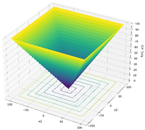
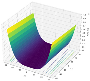
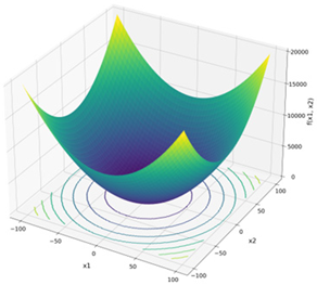
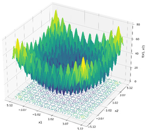
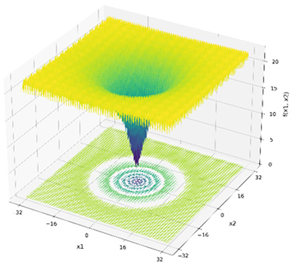
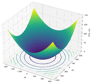
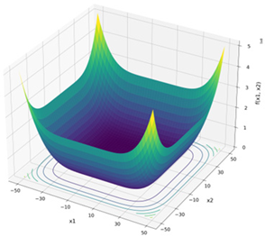
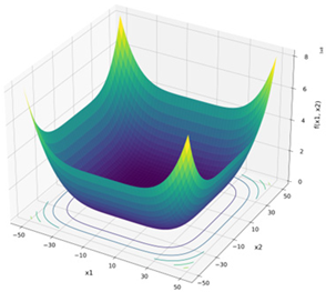
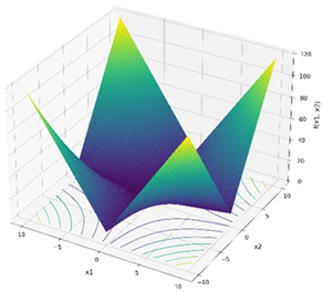
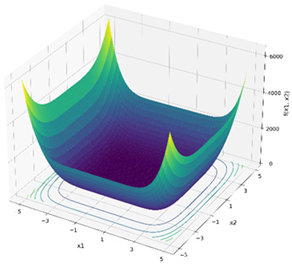
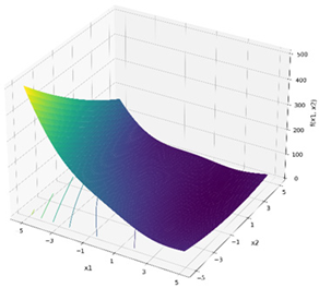
In Table 1, the Description column includes the functional expression and, as an example, the corresponding graph for the case of $n=2$. In addition, the Dimension column specifies the number of variables actually used in the experiments. The Range column indicates the domain of the variables applied in the experiments, and finally, the $f_{min}$ column presents the exact global optimum value.

Additionally, five real-world engineering design optimization problems, which feature constraints and complex interdependencies between variables, were used for testing [26,27]. These problems were classified separately, as the presence of multiple constraints makes them considerably more challenging optimization tasks compared to the general unimodal or multimodal problems listed above.

• F24—Welded beam design optimization problem

Figure 1 illustrates the overall structure of the welded beam design optimization problem and shows the meaning of each variable.

Minimize:

$$f\left(x\right)=1.10471x_1^2{x}_2+0.04811x_3{x}_4\left(14.0+x_2\right)$$

(4)

Subject to:

$$g_1\left(x\right)=\tau \left(x\right)-\mathrm{13,600}\le 0$$

(5)

$$g_2\left(x\right)=\sigma \left(x\right)-\mathrm{30,000}\le 0$$

(6)

$$g_3\left(x\right)=x_1-x_4\le 0$$

(7)

$$g_4\left(x\right)=0.10471x_1^2+0.04811x_3{x}_4\left(14+x_2\right)-5.0\le 0$$

(8)

$$g_5\left(x\right)=0.125-x_1\le 0$$

(9)

$$g_6\left(x\right)=\delta \left(x\right)-0.25\le 0$$

(10)

$$g_7\left(x\right)=6000-P_c\left(x\right)\le 0$$

(11)

With:

$$\tau \left(x\right)=\sqrt{{\left({\tau }^{\prime }\right)}^2+\left(2{\tau }^{\prime }{\tau }^{″}\right){\displaystyle \frac{x_2}{2R}}+{\left({\tau }^{″}\right)}^2}$$

(12)

$${\tau }^{\prime }={\displaystyle \frac{6000}{\sqrt{2}{x}_1{x}_2}},{\tau }^{″}={\displaystyle \frac{MR}{J}}$$

(13)

$$M=6000\left(14+{\displaystyle \frac{x_2}{2}}\right)$$

(14)

$$M=6000\left(14+{\displaystyle \frac{x_2}{2}}\right)$$

(15)

$$J=2\left\{x_1{x}_2\sqrt{2}\left[{\displaystyle \frac{x_2^2}{12}}+{\left({\displaystyle \frac{x_1+x_3}{2}}\right)}^2\right]\right\}$$

(16)

$$\sigma \left(x\right)={\displaystyle \frac{\mathrm{504,000}}{x_4{x}_3^2}}$$

(17)

$$\delta \left(x\right)={\displaystyle \frac{\mathrm{65,856,000}}{\left(30\times {10}^6\right)x_4{x}_3^3}}$$

(18)

$$P_c\left(x\right)={\displaystyle \frac{4.013\left(30\times {10}^6\right)\sqrt{\frac{x_3^2{x}_4^6}{36}}}{196}}\left(1-{\displaystyle \frac{x_3\sqrt{\frac{30\times {10}^6}{4\left(12\times {10}^6\right)}}}{28}}\right)$$

(19)

where $0.1\le x_1,x_4\le 2.0,0.1\le x_2,x_3\le 10.0$

• F25—Tension/compression spring design optimization problem

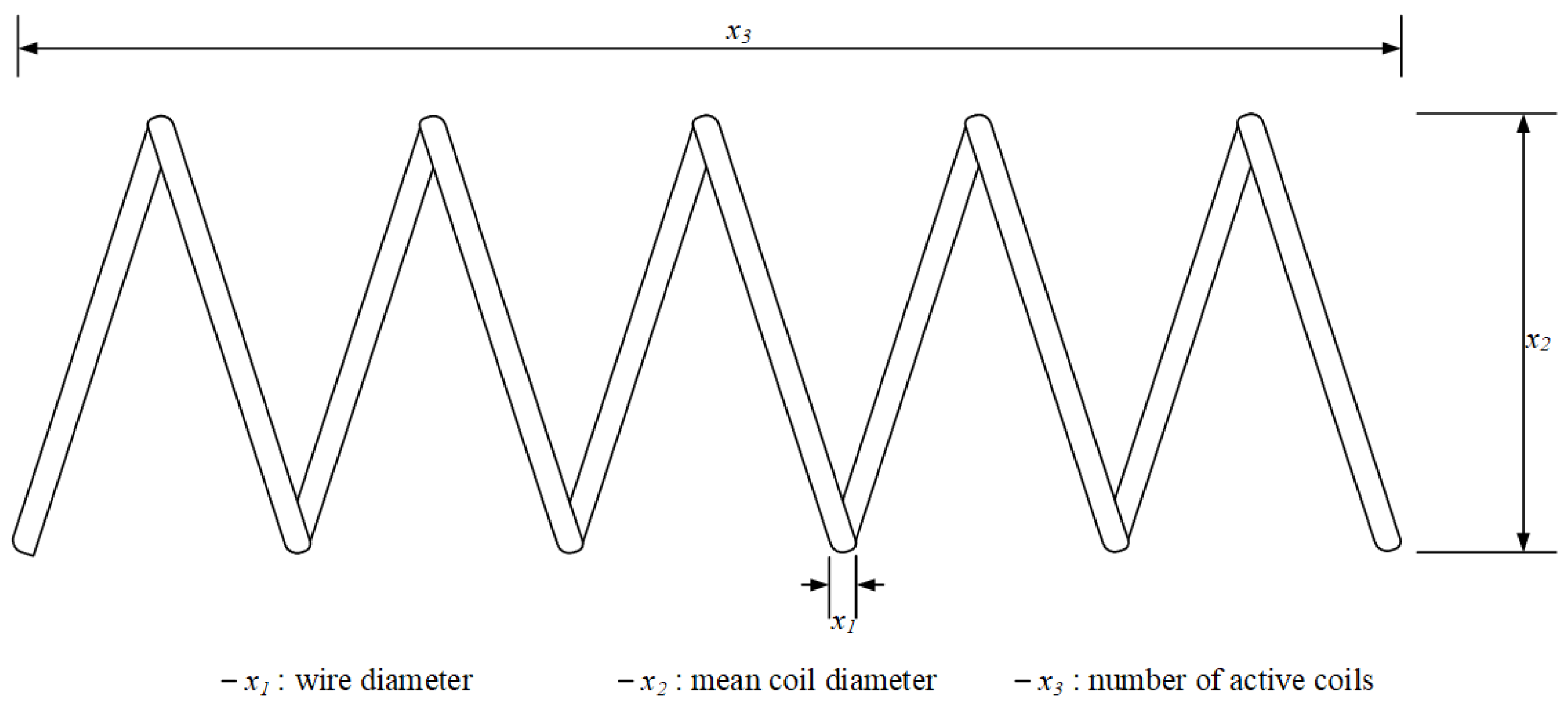
Figure 2 illustrates the overall structure of the tension/compression spring design optimization problem and shows the meaning of each variable.

Minimize:

$$f\left(x\right)=\left(x_3+2\right)x_2{x}_1^2$$

(20)

Subject to:

$$g_1\left(x\right)=1-{\displaystyle \frac{x_2^3{x}_3}{\mathrm{71,785}{x}_1^4}}\le 0$$

(21)

$$g_2\left(x\right)={\displaystyle \frac{4x_2^2-x_1{x}_2}{\mathrm{12,566}\left(x_2{x}_1^3-x_1^4\right)}}+{\displaystyle \frac{1}{5108x_1^2}}-1\le 0$$

(22)

$$g_3\left(x\right)=1-{\displaystyle \frac{140.45x_1}{x_2^2{x}_3}}\le 0$$

(23)

$$g_4\left(x\right)={\displaystyle \frac{x_1+x_2}{1.5}}-1\le 0$$

(24)

where $0.05\le x_1\le 2.0,0.25\le x_2\le 1.3,2.0\le x_3\le 15.0$.

• F26—Pressure vessel design optimization problem

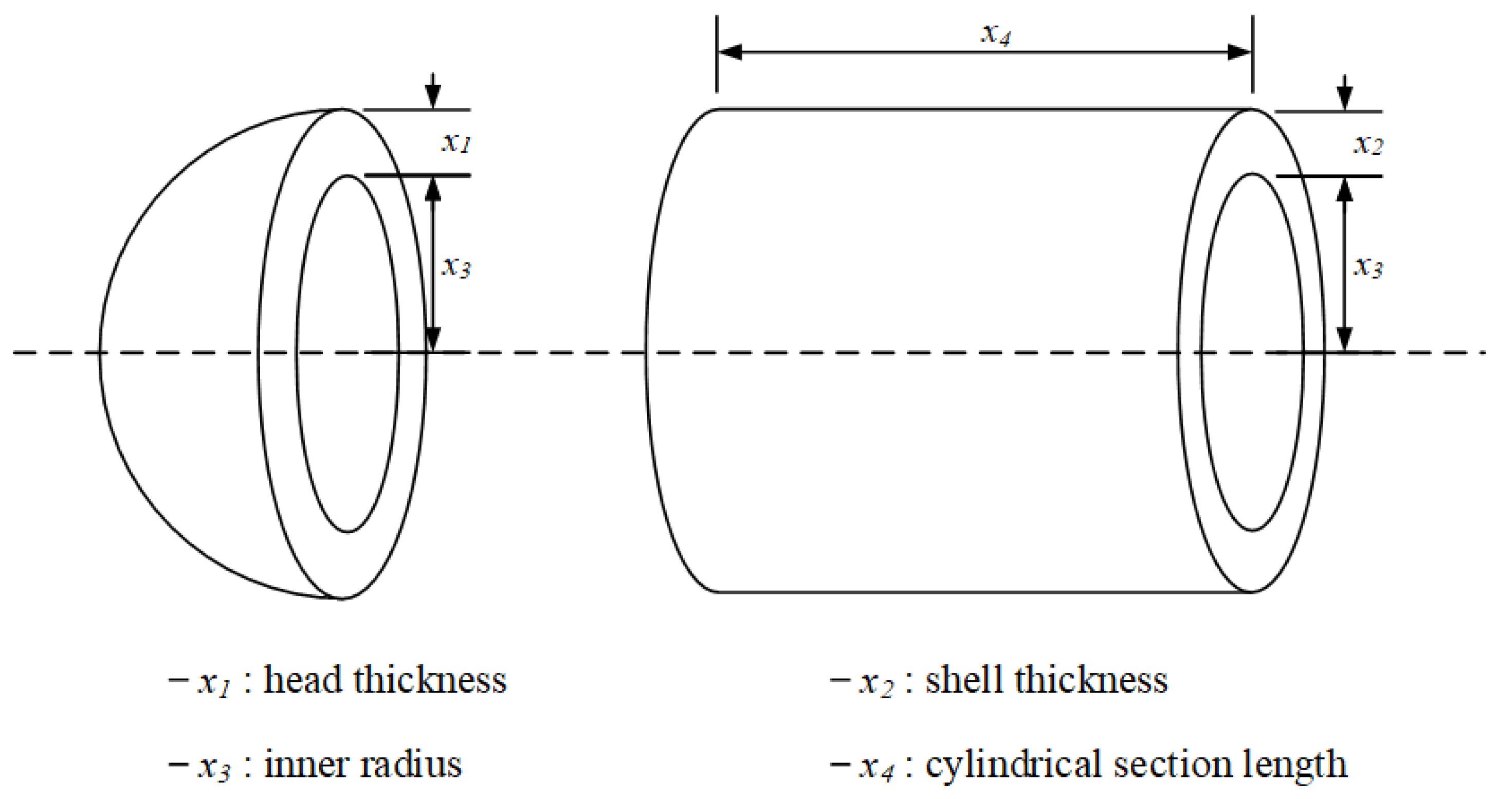
Figure 3 illustrates the overall structure of the pressure vessel design optimization problem and shows the meaning of each variable.

Minimize:

$$f\left(x\right)=0.6224x_1{x}_3{x}_4+1.7781x_2{x}_3^2+3.1661x_1^2{x}_4+19.84x_1^2{x}_3$$

(25)

Subject to:

$$g_1\left(x\right)=-x_1+0.0193x_3\le 0$$

(26)

$$g_2\left(x\right)=-x_2+0.00954x_3\le 0$$

(27)

$$g_3\left(x\right)=-\pi x_3^2{x}_4^2-{\displaystyle \frac{4}{3}}\pi x_3^3+\mathrm{1,296,000}\le 0$$

(28)

$$g_4\left(x\right)=x_4-240\le 0$$

(29)

where $0.0625\times 1\le x_1,x_2\le 0.0625\times 99,10.0\le x_3,x_4\le 200.0$

• F27—3bar truss design optimization problem

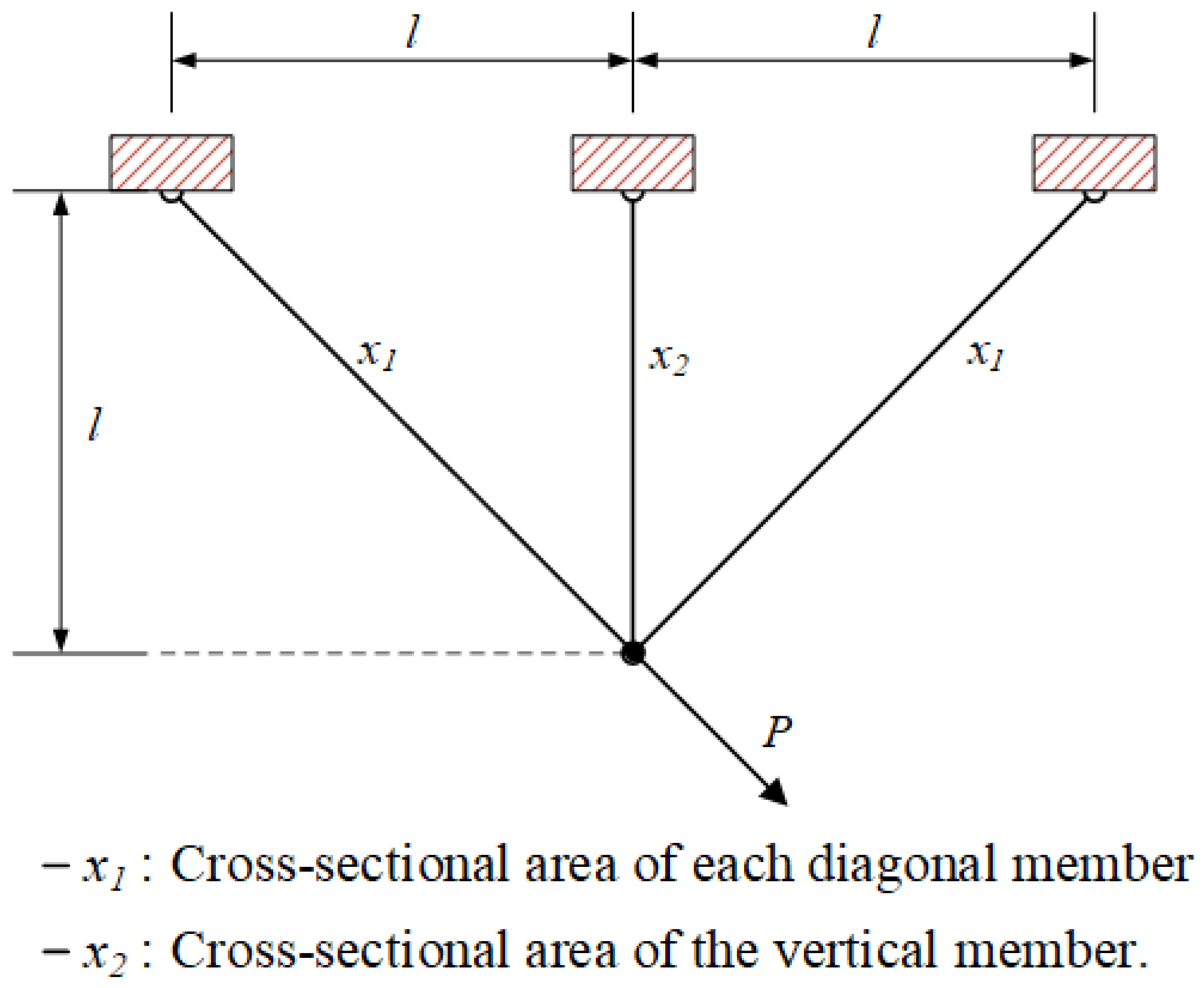
Figure 4 illustrates the overall structure of the 3bar truss design optimization problem. and shows the meaning of each variable.

Minimize:

$$f\left(x\right)=\left(2\sqrt{2}{x}_1+x_2\right)\times l$$

(30)

Subject to:

$$g_1\left(x\right)={\displaystyle \frac{\sqrt{2}{x}_1+x_2}{\sqrt{2}{x}_1^2+2x_1{x}_2}}P-\sigma \le 0$$

(31)

$$g_2\left(x\right)={\displaystyle \frac{x_2}{\sqrt{2}{x}_1^2+2x_1{x}_2}}P-\sigma \le 0$$

(32)

$$g_3\left(x\right)={\displaystyle \frac{1}{\sqrt{2}{x}_2+x_1}}P-\sigma \le 0$$

(33)

With:

$$l=100\mathrm{c}\mathrm{m},P=2\mathrm{k}\mathrm{N}/{\mathrm{c}\mathrm{m}}^2,\sigma =2\mathrm{k}\mathrm{N}/{\mathrm{c}\mathrm{m}}^2$$

where $0.0\le {\mathrm{x}}_1,{\mathrm{x}}_2\le 1.0$

• F28—Speed reducer design optimization problem

Figure 5 illustrates the overall structure of speed reducer design optimization problem and shows the meaning of each variable.

Minimize:

$$f\left(x\right)=0.7854x_1{x}_2^2\left(3.3333x_3^2+14.9334x_3-43.0934\right)-1.508x_1\left(x_6^2+x_7^2\right)+7.4777\left(x_6^3+x_7^3\right)+0.7854\left(x_4{x}_6^2+{x_{5}x}_7^2\right)$$

(34)

Subject to:

$$g_1\left(x\right)={\displaystyle \frac{27}{x_1{x}_2^2{x}_3}}-1\le 0$$

(35)

$$g_2\left(x\right)={\displaystyle \frac{397.5}{x_1{x}_2^2{x}_3^2}}-1\le 0$$

(36)

$$g_3\left(x\right)={\displaystyle \frac{1.93x_4^3}{x_2{x}_3{x}_6^4}}-1\le 0$$

(37)

$$g_4\left(x\right)={\displaystyle \frac{1.93x_5^3}{x_2{x}_3{x}_7^4}}-1\le 0$$

(38)

$$g_5\left(x\right)={\displaystyle \frac{1.0}{110x_6^3}}\sqrt{{\left({\displaystyle \frac{745.0x_4}{x_2{x}_3}}\right)}^2+16.9\times {10}^6}-1\le 0$$

(39)

$$g_6\left(x\right)={\displaystyle \frac{1.0}{85x_7^3}}\sqrt{{\left({\displaystyle \frac{745.0x_5}{x_2{x}_3}}\right)}^2+157.5\times {10}^6}-1\le 0$$

(40)

$$g_7\left(x\right)={\displaystyle \frac{x_2{x}_3}{40}}-1\le 0$$

(41)

$$g_8\left(x\right)={\displaystyle \frac{{5x}_2}{x_1}}-1\le 0$$

(42)

$$g_9\left(x\right)={\displaystyle \frac{x_1}{12x_2}}-1\le 0$$

(43)

$$g_{10}\left(x\right)={\displaystyle \frac{1.5x_6+1.9}{x_4}}-1\le 0$$

(44)

$$g_{11}\left(x\right)={\displaystyle \frac{{1.1x}_7+1.9}{x_5}}-1\le 0$$

(45)

where $2.6\le x_1\le 3.6,0.7\le x_2\le 0.8,17\le x_3\le 28,7.3\le x_4\le 8.3,7.8\le x_5\le 8.3,2.9\le x_6\le 3.9,5.0\le x_7\le 5.5$.

3.2. Experimental Design and Performance Evaluation

In this study, to primarily investigate the influence of the HMCR and PAR parameters, which govern the core operators of the algorithm, the remaining parameters such as HMS and NI were fixed to values commonly adopted in previous studies.

All experiments were performed in Microsoft Excel using VBA, and comprehensive details of the experimental environment, including hardware specifications, are available in the Supplementary Materials.

For F24–28, which involve constraints, these were handled by adding a penalty term to the objective function, as expressed in the formulation used in Equation (46).

$$\mathrm{F}\left(\mathrm{x}\right)=\mathrm{f}\left(\mathrm{x}\right)+\sum _{i=1}^n{R}_i·max{\left(0,g_i\left(x\right)\right)}^2+\mathrm{C}$$

(46)

Here, $f\left(x\right)$ denotes the original objective function, $R_i$ the penalty coefficient, $g_i\left(x\right)$ the constraint, and $C$ the constant term. In this study, for F24, the penalty coefficient $R_i$ was set to 100 and the constant term $C$ was set to 1000. These values were chosen so that the magnitude of the penalty term would be considerably larger than that of the original objective function $f\left(x\right)$, thereby making it more likely that solutions satisfying all constraints would remain in the HM.

The experiment was designed as follows to precisely measure the algorithm’s parameter sensitivity.

• Variable Parameters:

HMCR: 0.0, 0.1, 0.2, …, 1.0 (11 levels)

PAR: 0.0, 0.1, 0.2, …, 1.0 (11 levels)

were conducted for a total of 11 × 11 = 121 parameter combinations.

• Fixed Parameters:

HMS: 30

Number of Improvisations (NI): 30,000

Maximum PA Step($bw$): $(x_{UB}-x_{LB})/\mathrm{30,000}$

• Performance Evaluation:

For each benchmark function and each of the 121 parameter combinations, the HS algorithm was executed independently 30 times. To ensure statistical reliability, the average of the objective function values from the 30 runs was considered the final performance for that combination. Subsequently, the performance values of the 121 combinations were ranked. A rank closer to 1 indicates a better-performing parameter combination.

• Visualization:

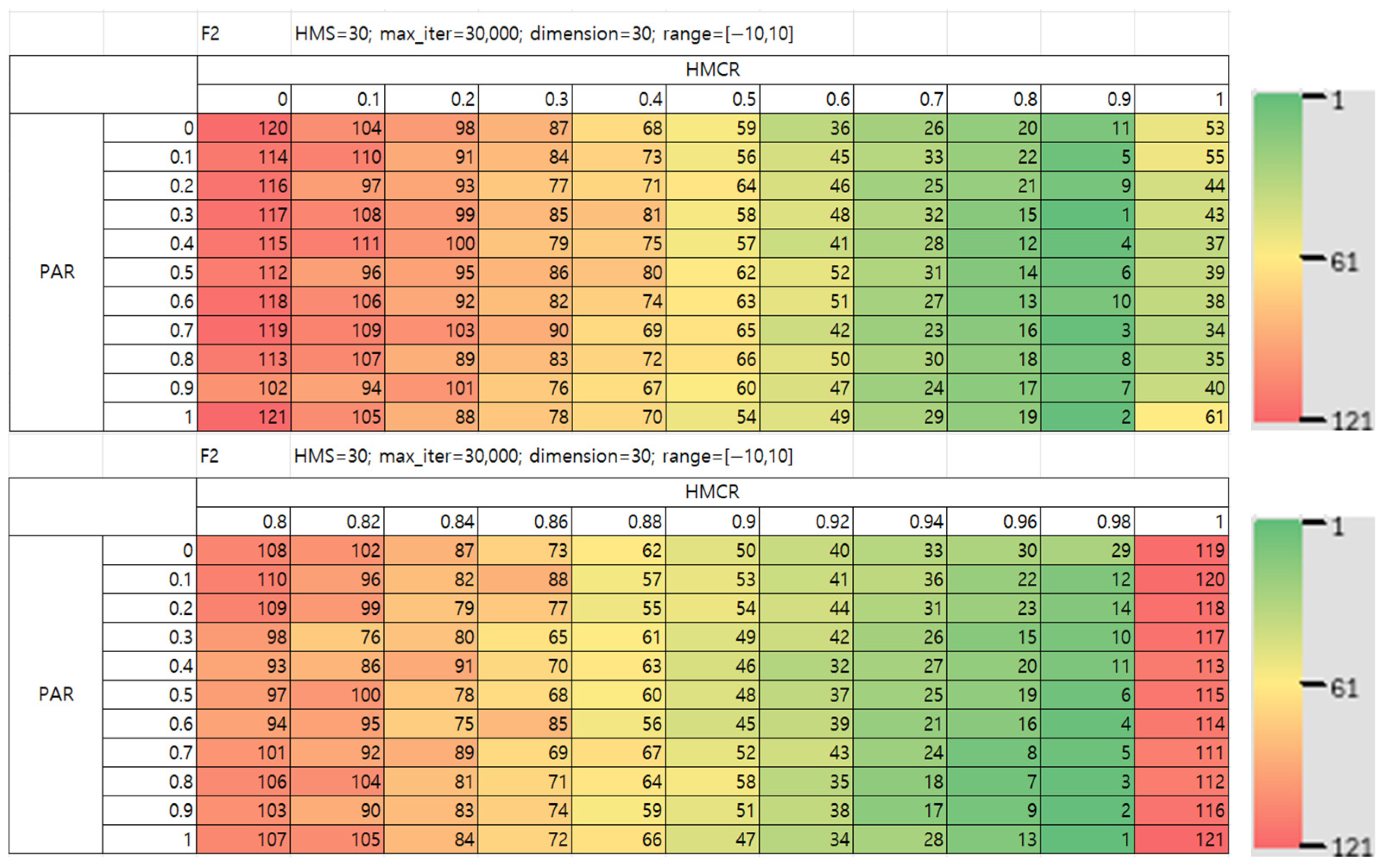
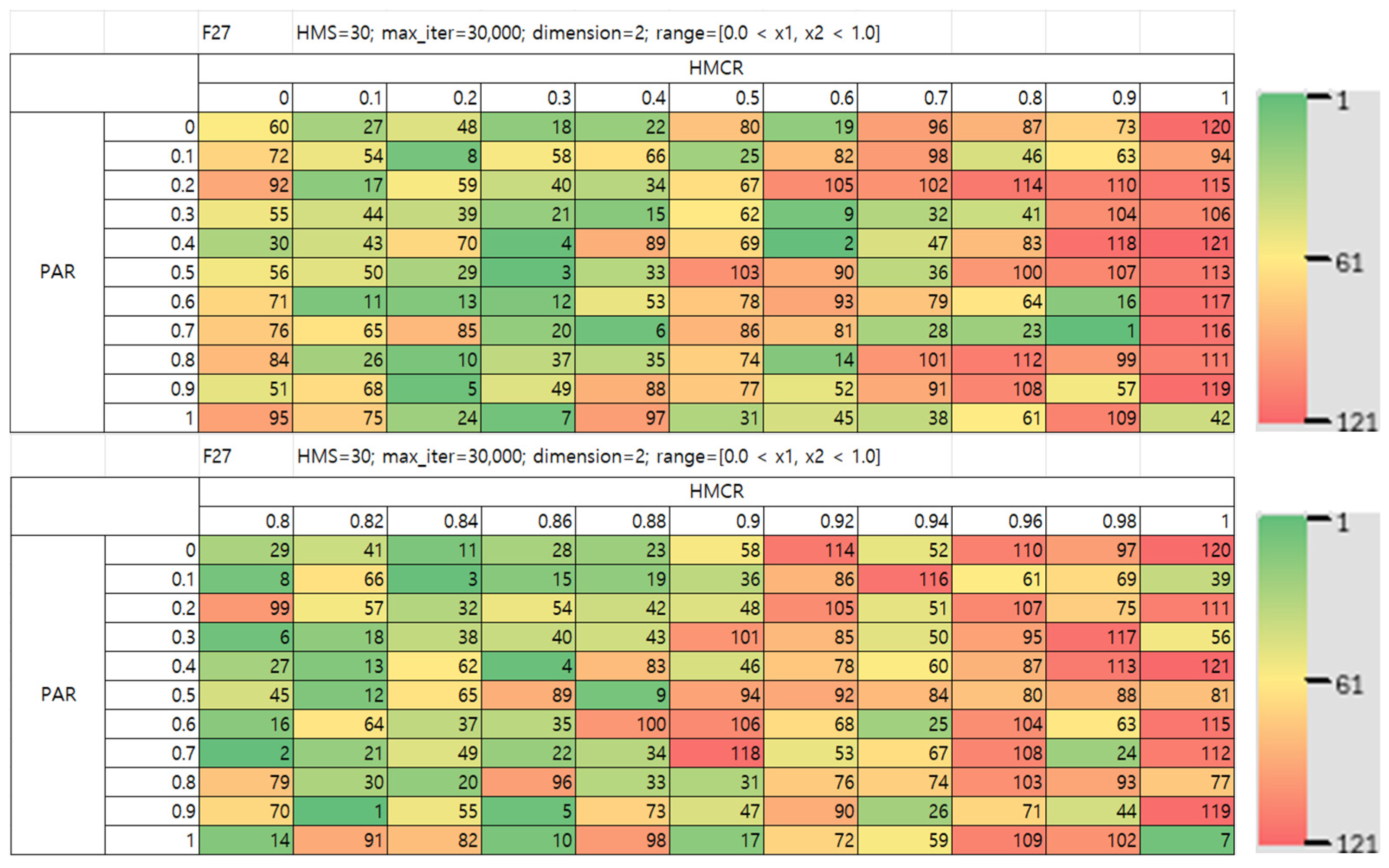
To facilitate an intuitive assessment of parameter sensitivity, the performance ranks of the 121 parameter combinations for each function were visualized as an 11 × 11 heatmap. In these heatmaps, the axes correspond to the PAR and HMCR values, while the color of each cell represents the performance rank. A green color scale signifies a high rank (superior performance), whereas a red scale indicates a low rank (inferior performance). This visualization scheme allows for the direct visual identification of parameter sensitivity, as illustrated in the example in Figure 6.

A preliminary empirical analysis of the results for several benchmark functions revealed that the algorithm’s performance is highly sensitive to the HMCR parameter. Specifically, a strong trend was observed wherein optimal performance was generally achieved with an HMCR value of 0.9. Therefore, to conduct a more granular investigation of the performance characteristics in the vicinity of HMCR = 0.9, a subsequent experiment was conducted as follows.

• Variable Parameters:
  HMCR: 0.82, 0.84, 0.86, …, 0.98 (9 levels)
  PAR: 0.0, 0.1, 0.2, …, 1.0 (11 levels)
  Other conditions are the same as before, and additional experiments are performed for a total of 9 × 11 = 99 parameter combinations.

4. Results and Analysis

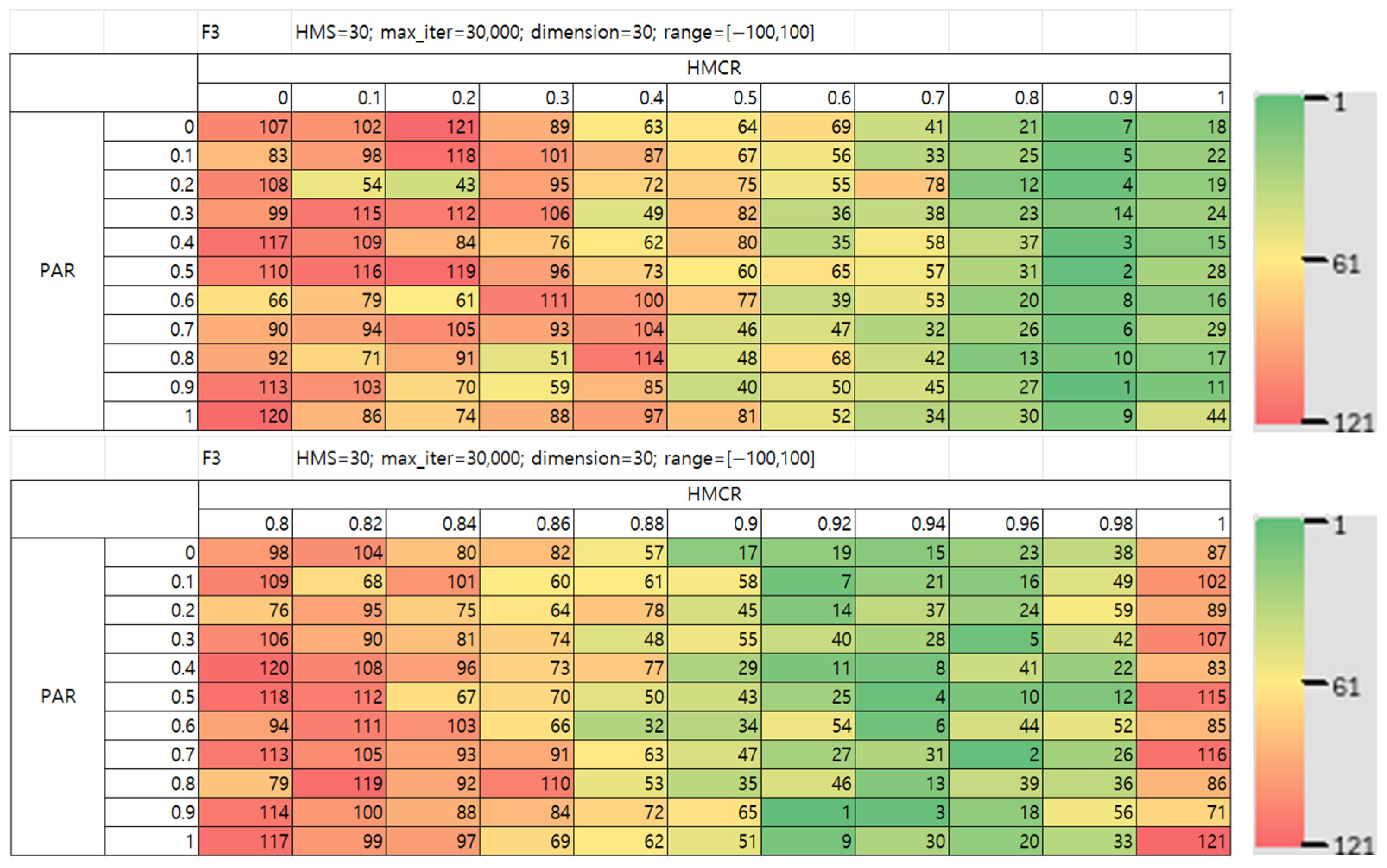
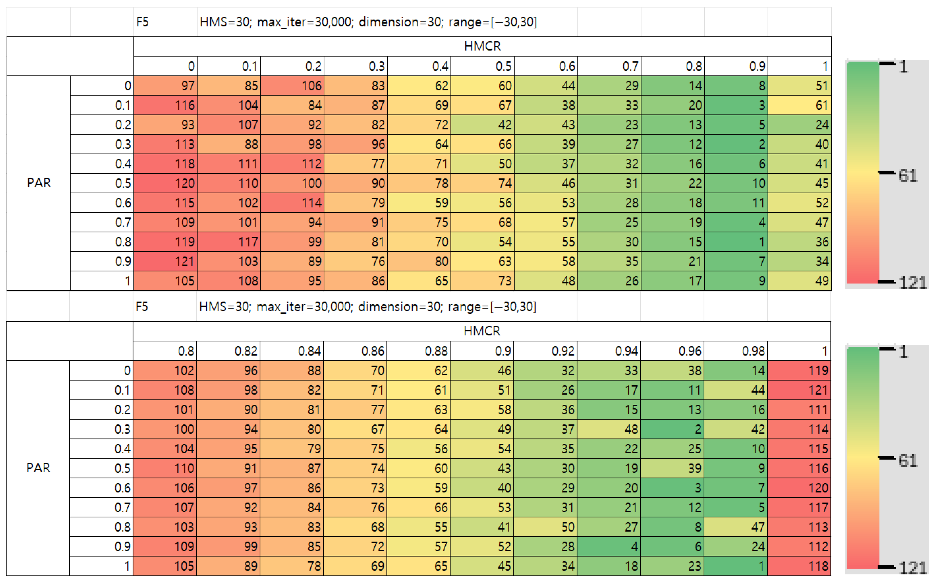
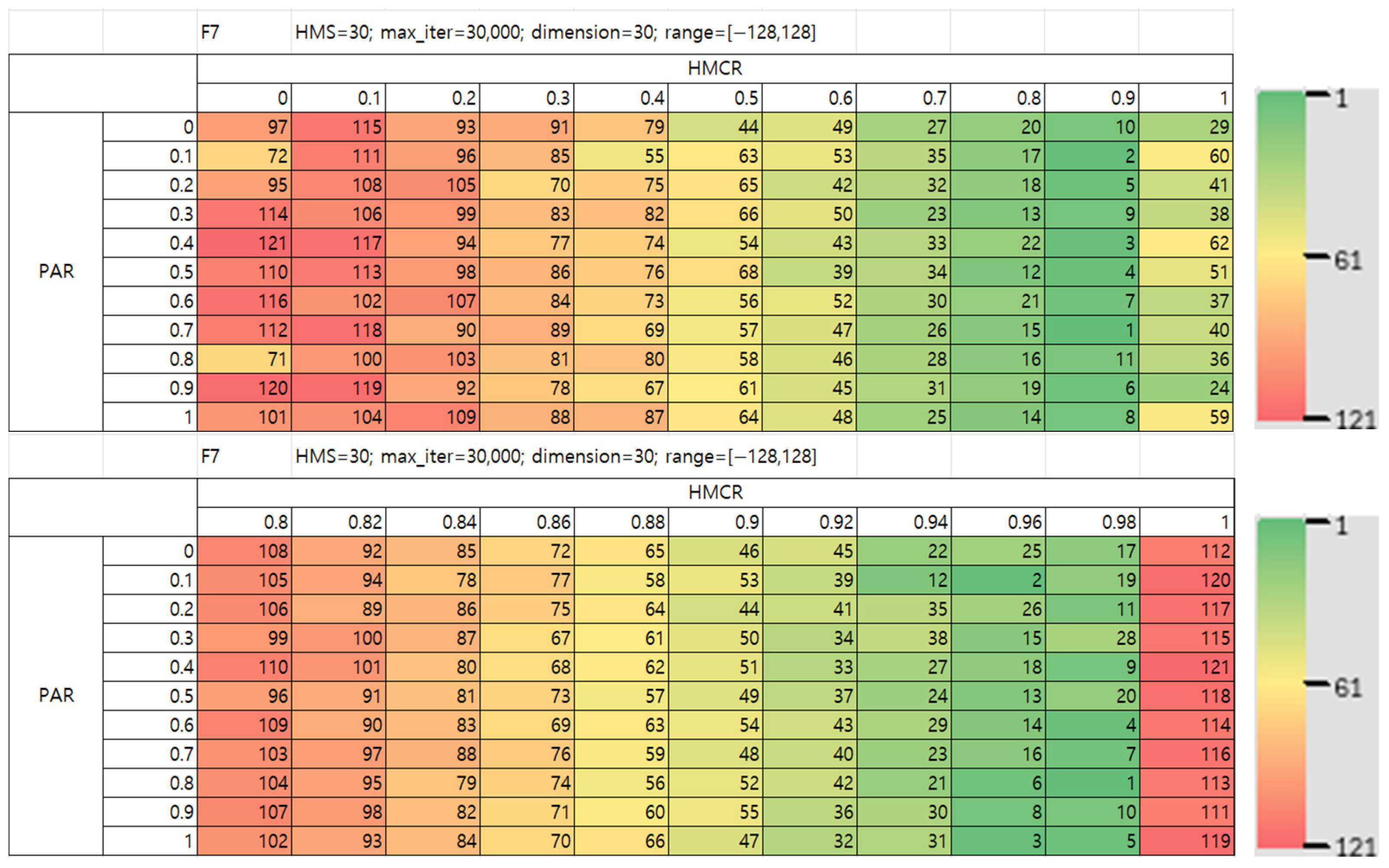
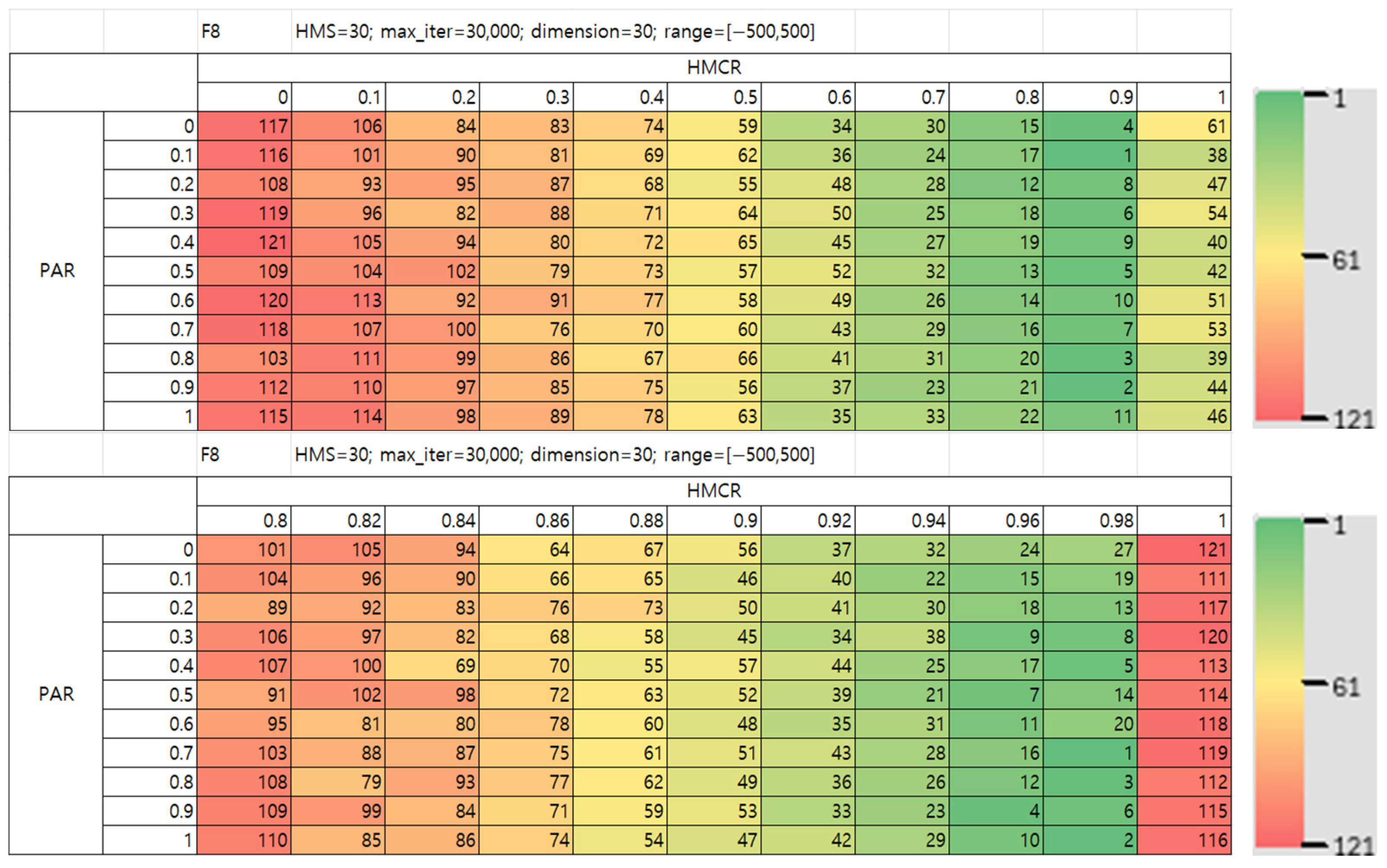
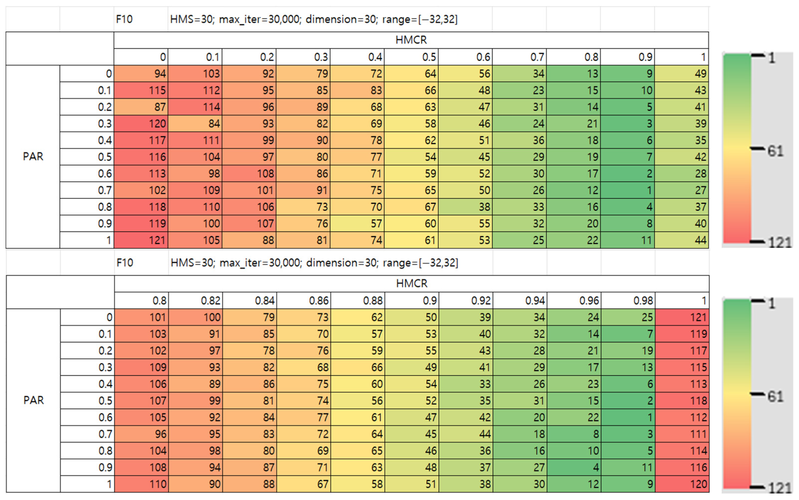
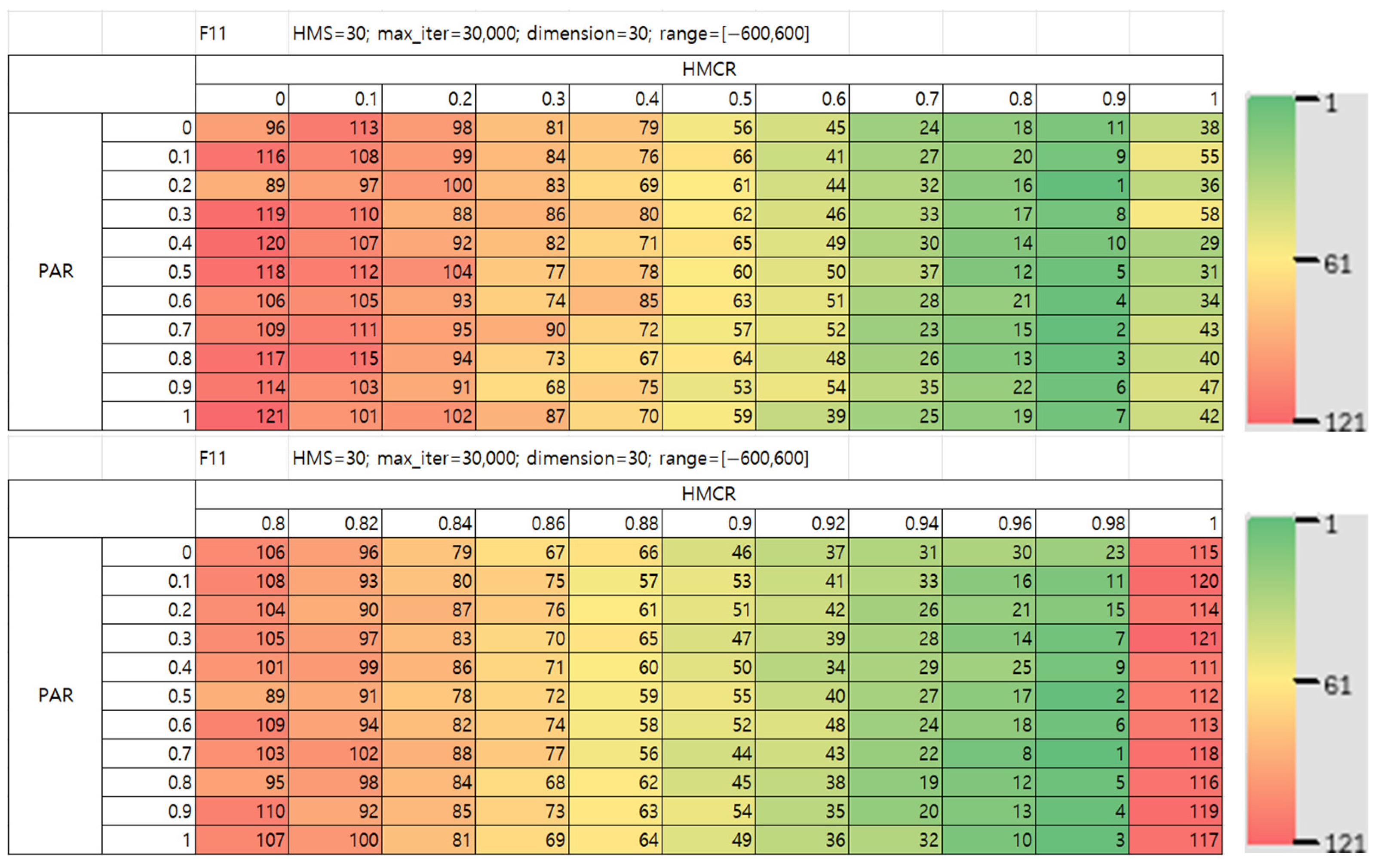
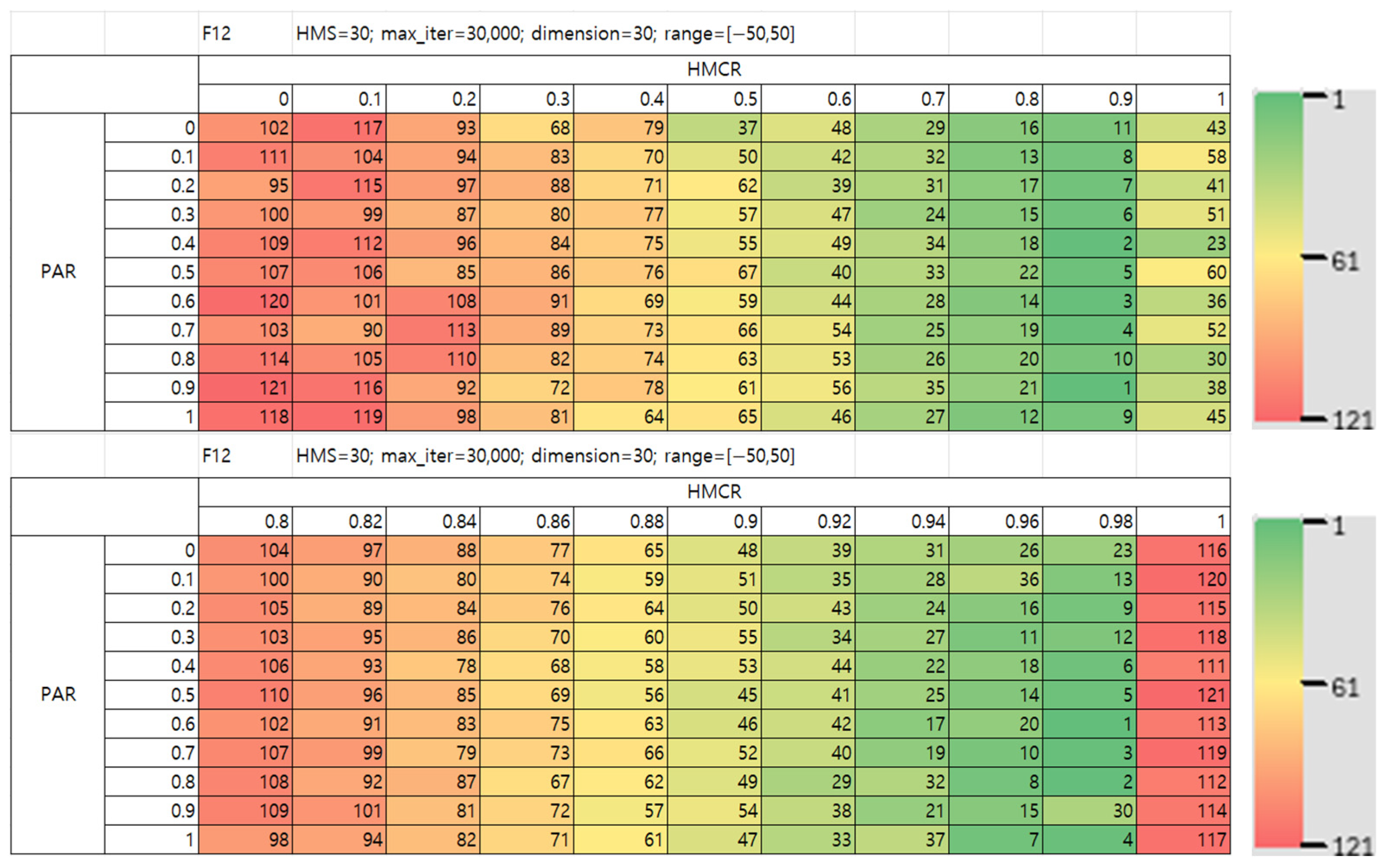
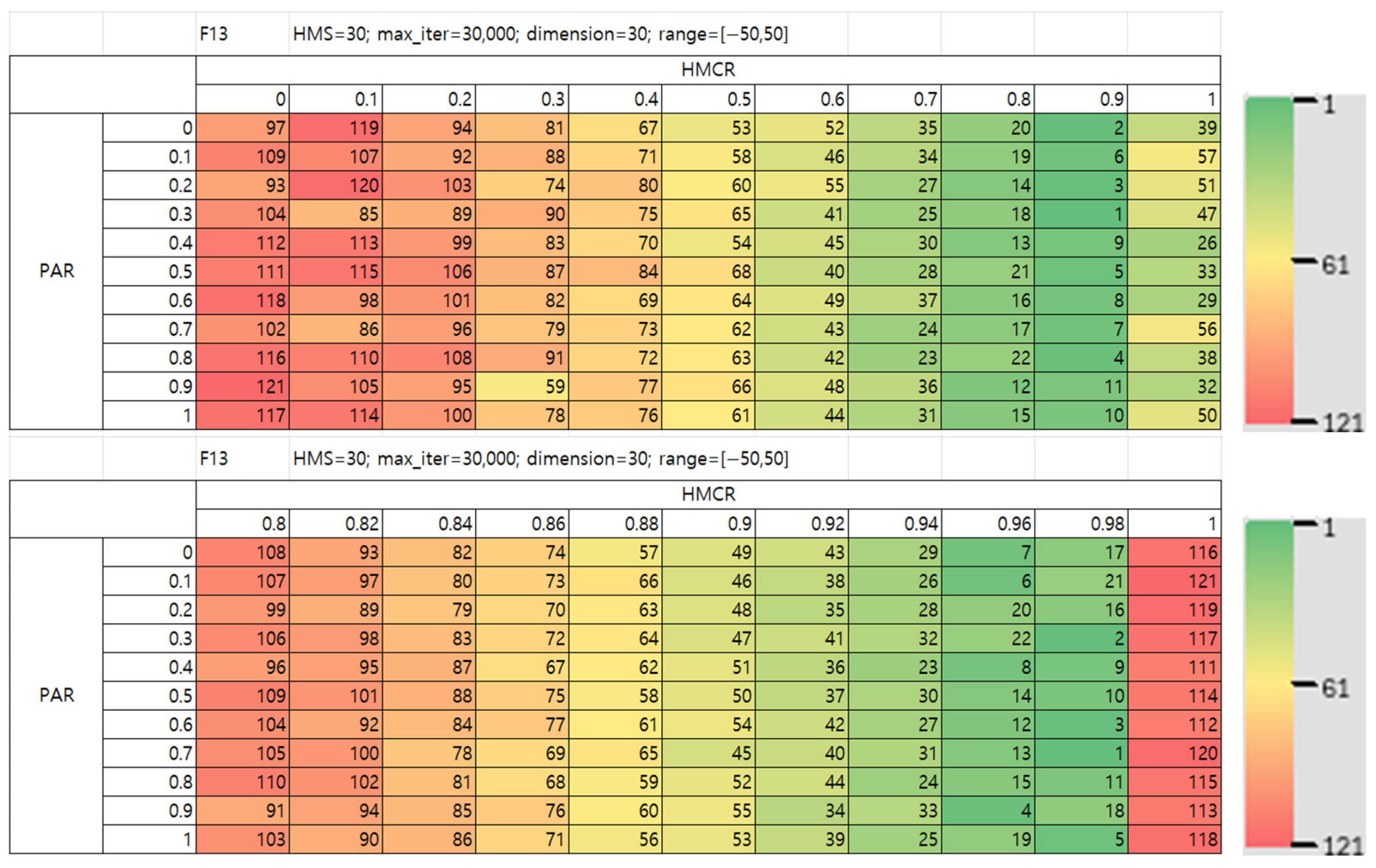
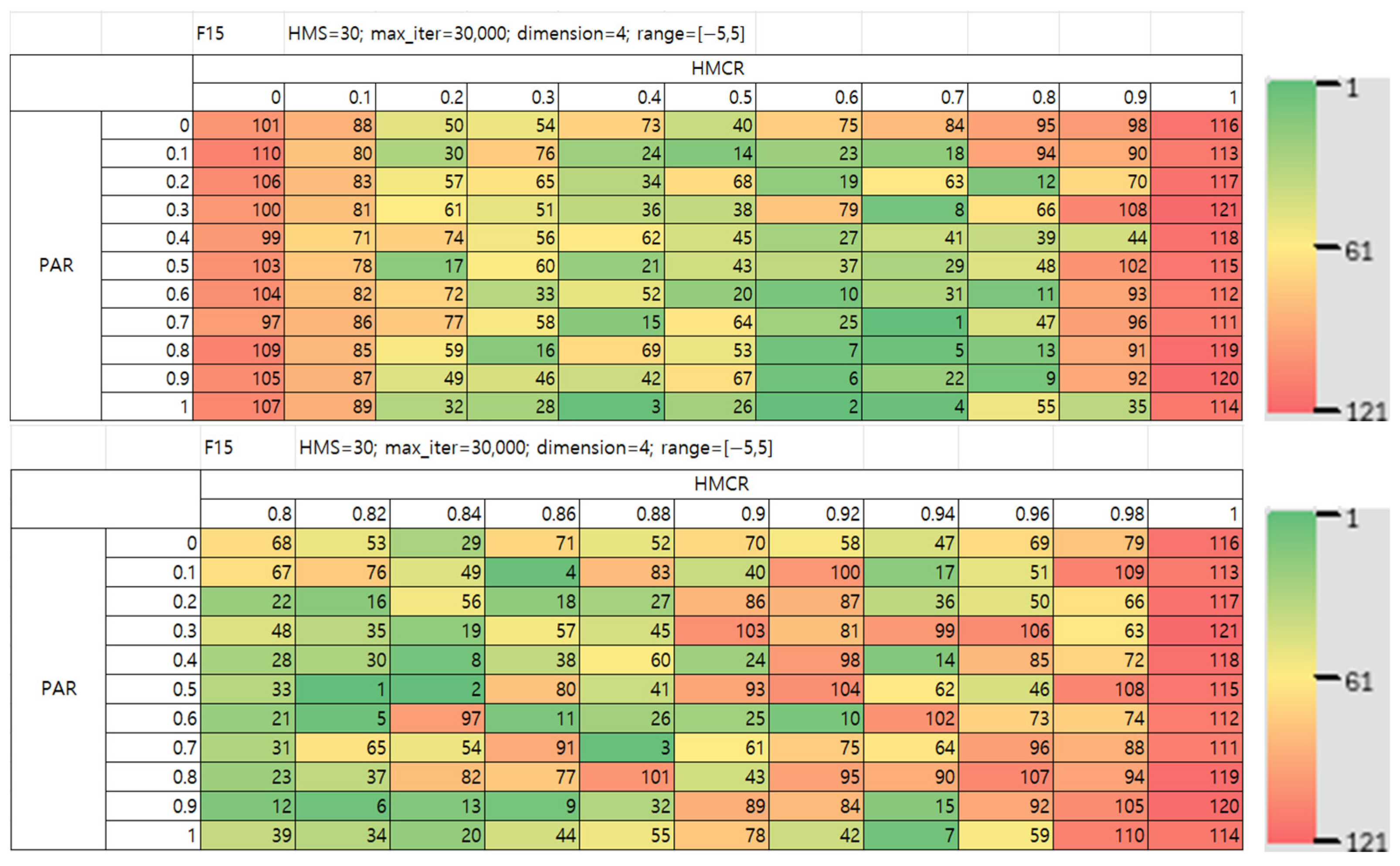
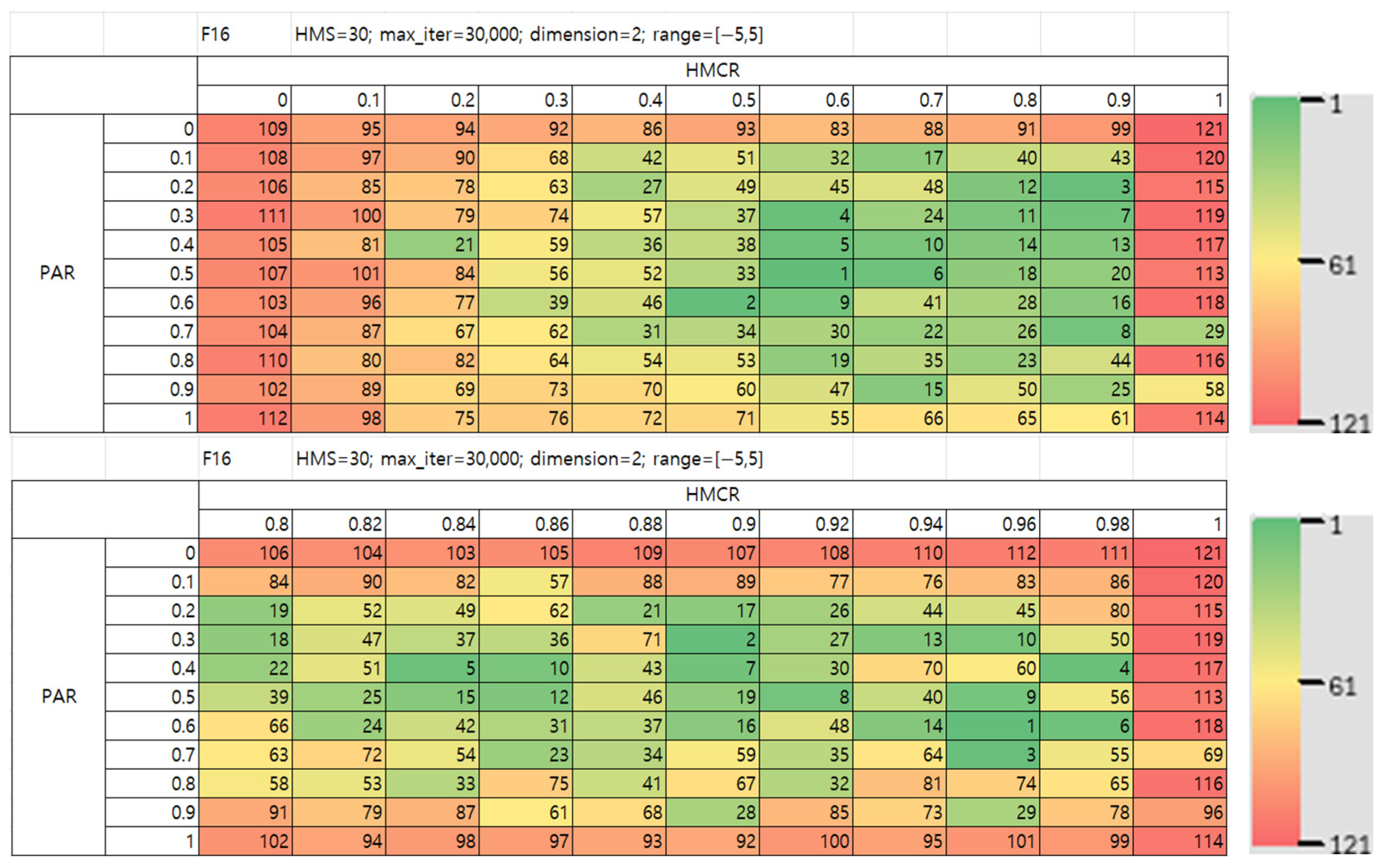
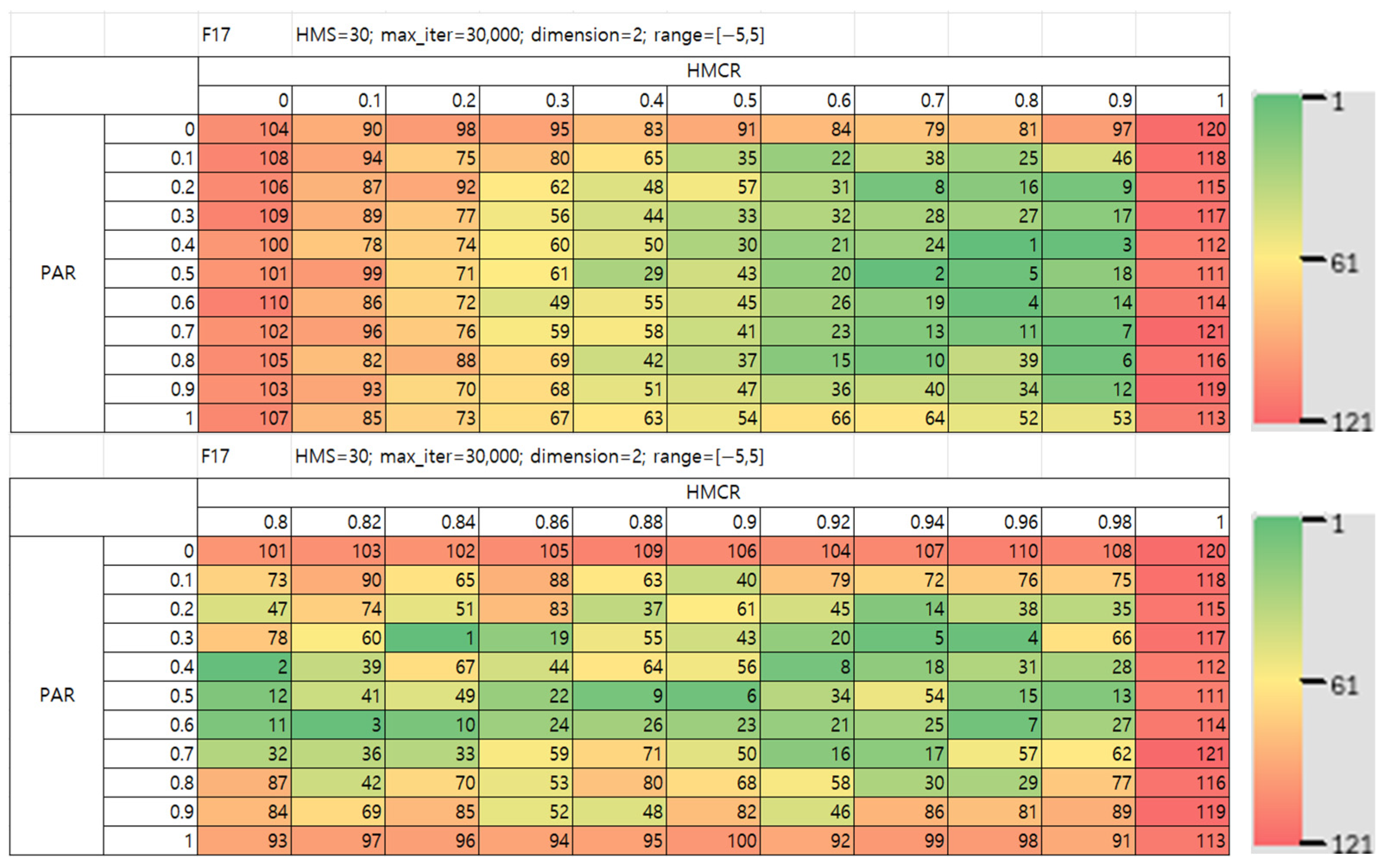
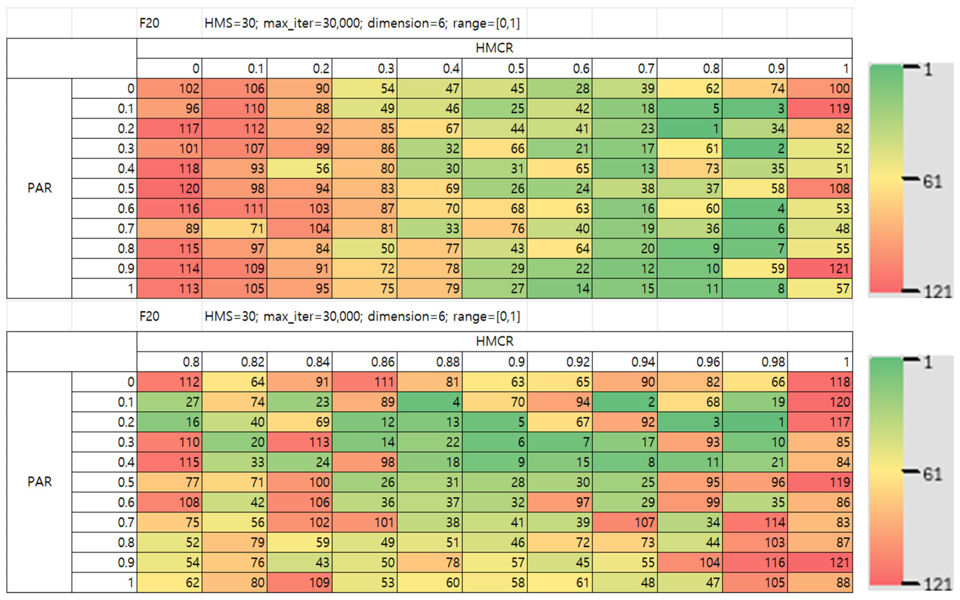
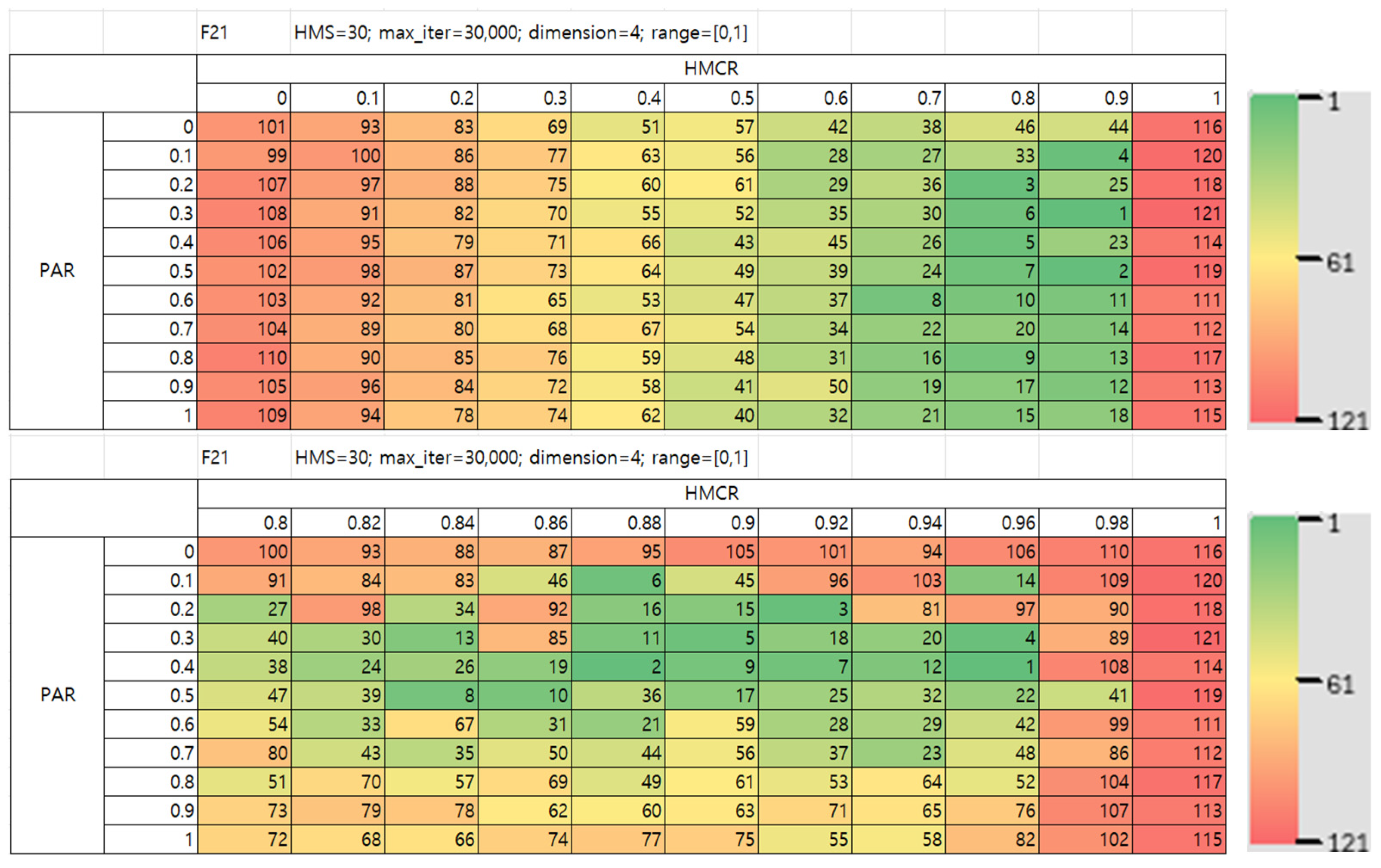
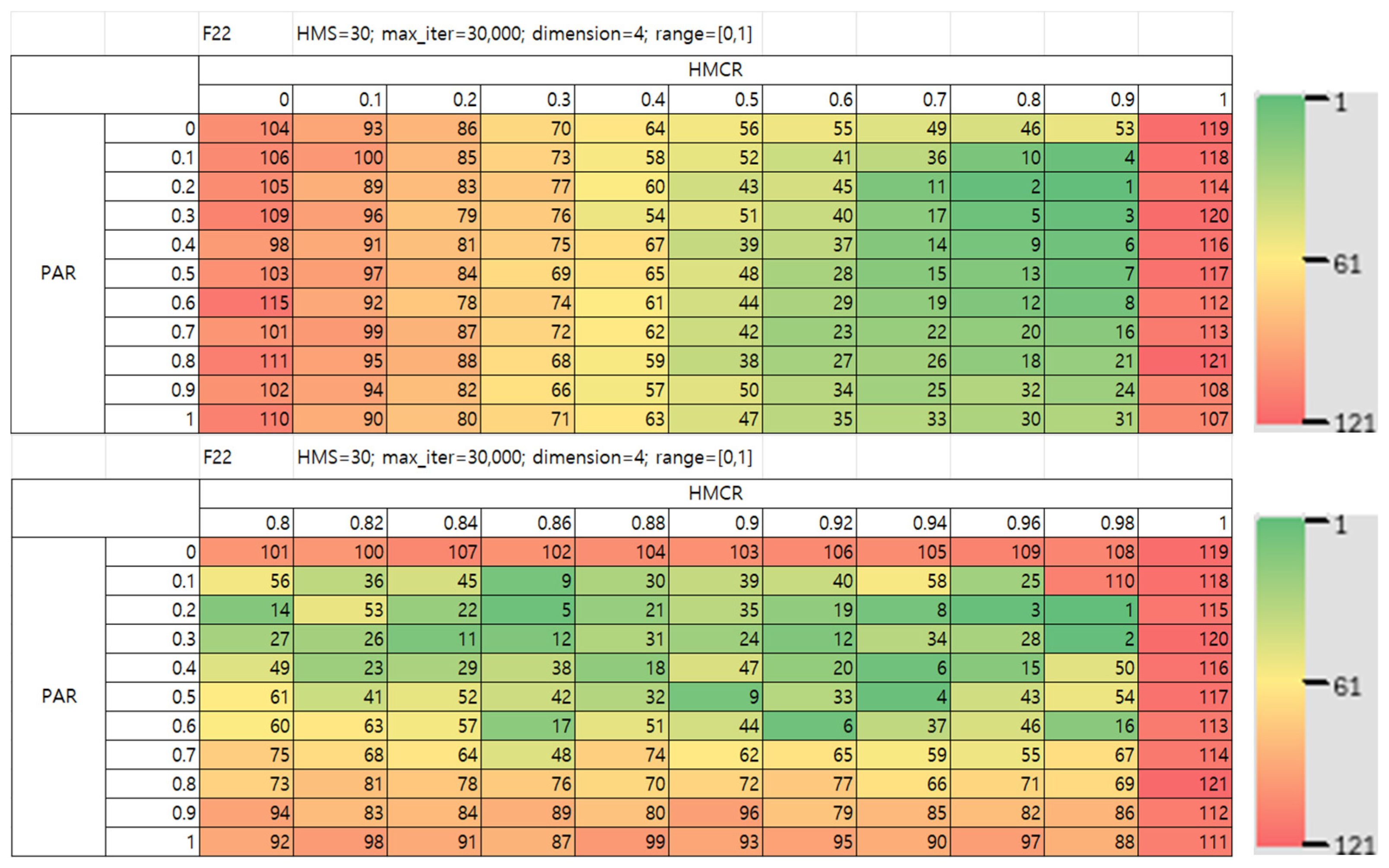
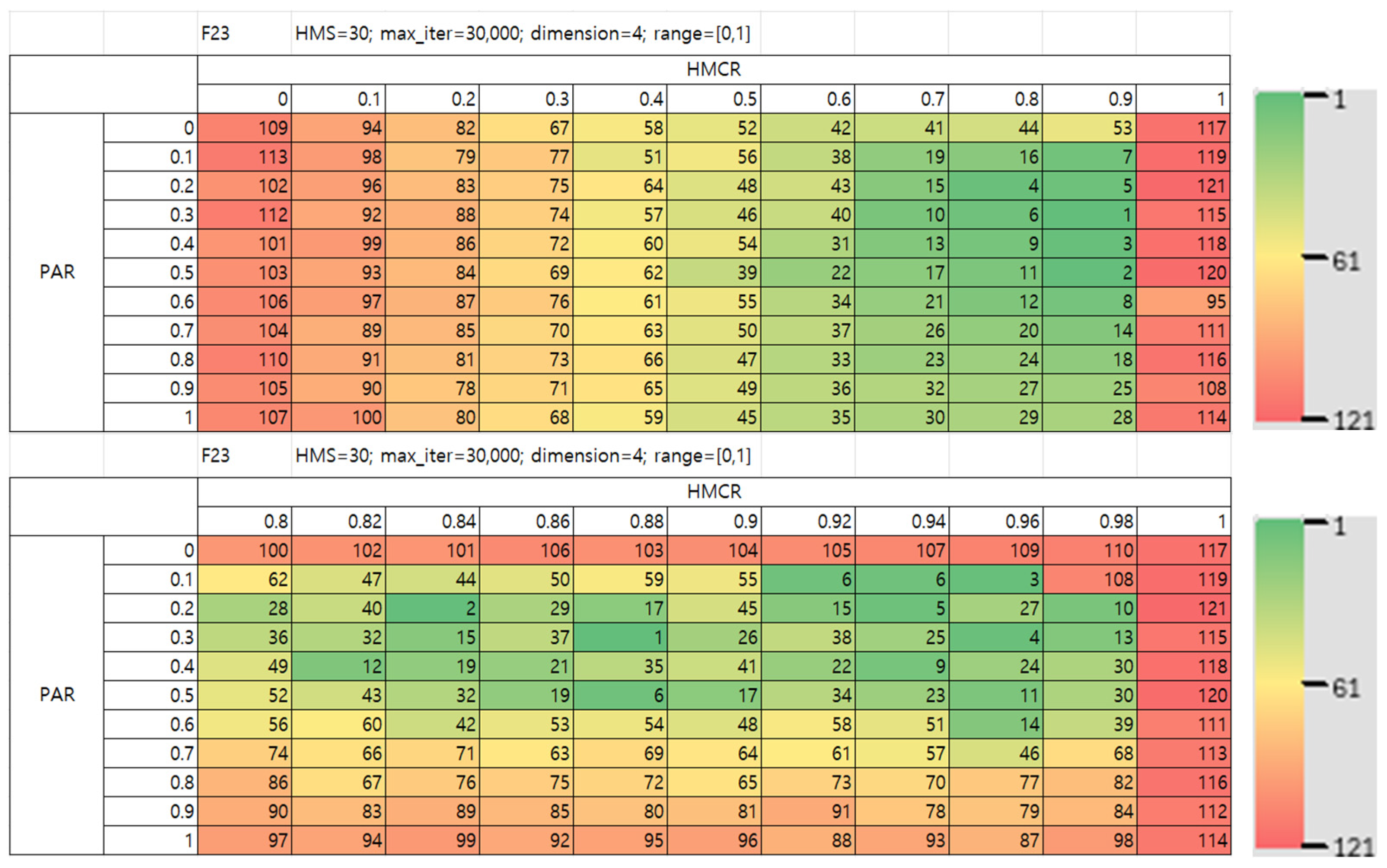
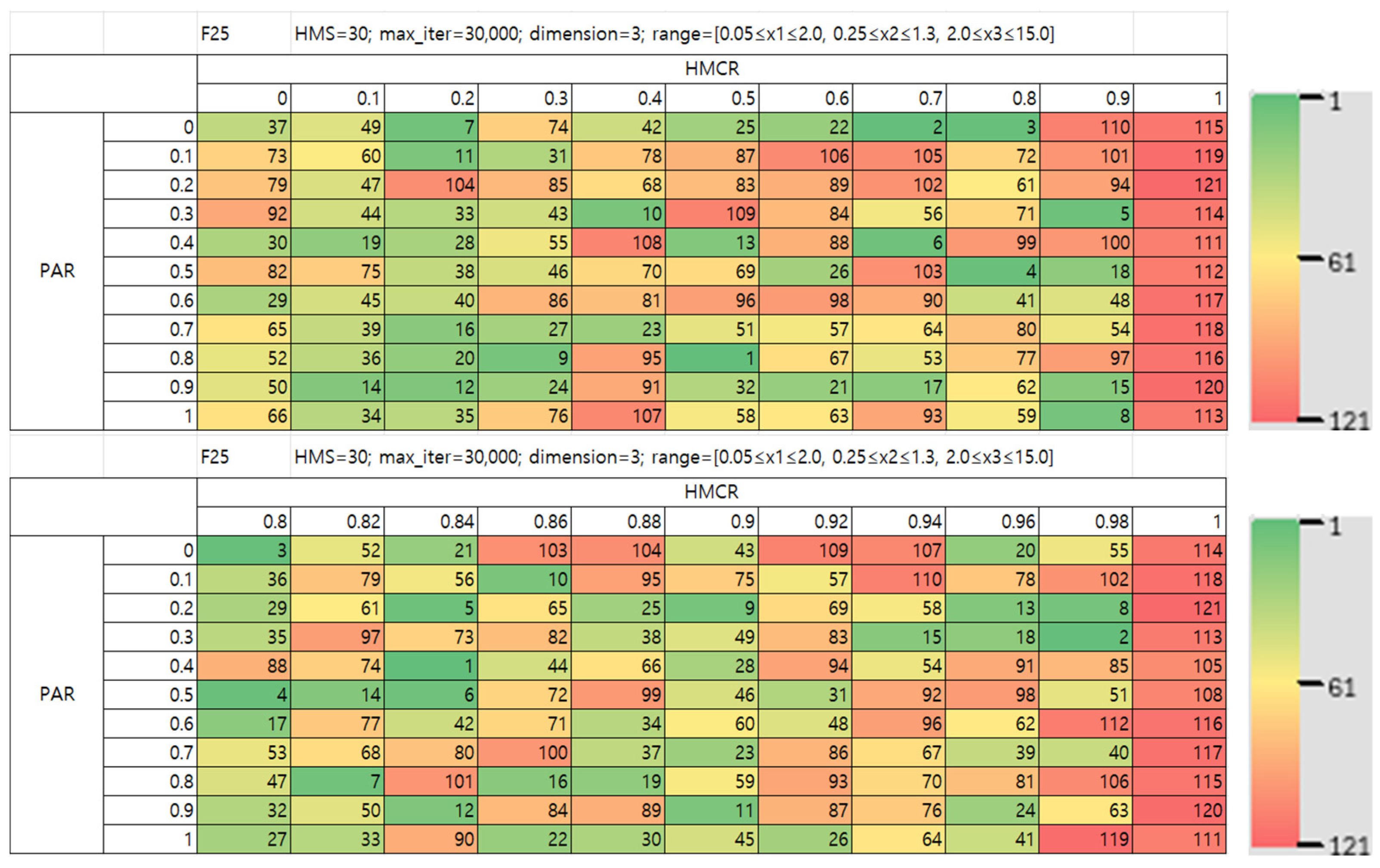
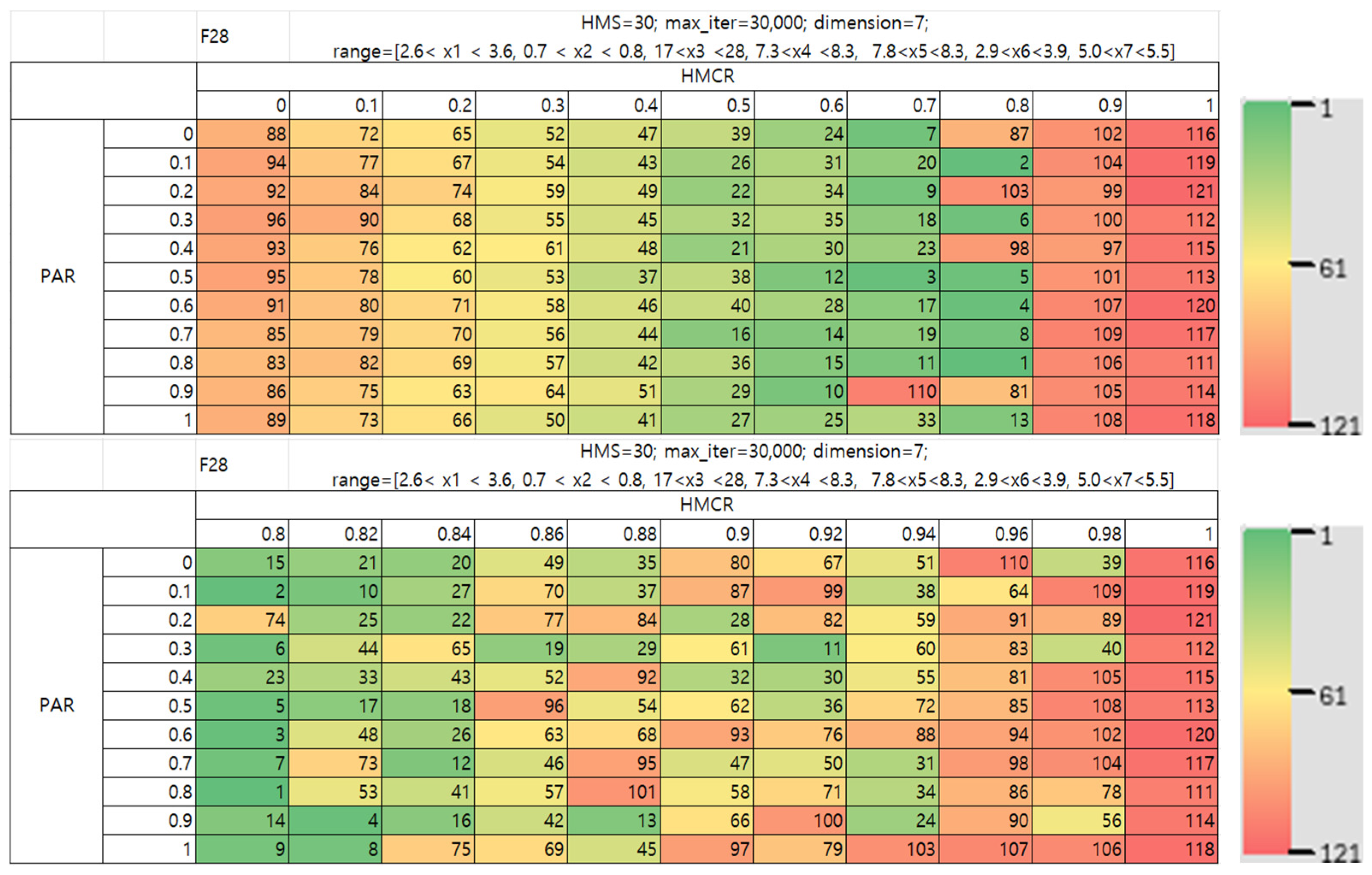
The sensitivity analysis results of two hyper-parameters (HMCR and PAR) for unconstrained unimodal functions (F1–F7), multimodal functions (F8–F23) and real-world design problems (F24–F28) are displayed in Figure 7, Figure 8, Figure 9, Figure 10, Figure 11, Figure 12, Figure 13, Figure 14, Figure 15, Figure 16, Figure 17, Figure 18, Figure 19, Figure 20, Figure 21, Figure 22, Figure 23, Figure 24, Figure 25, Figure 26, Figure 27, Figure 28, Figure 29, Figure 30, Figure 31, Figure 32, Figure 33 and Figure 34 in the form of heatmaps.

4.1. Overall Trends in Parameter Sensitivity

In Figure 7, Figure 8, Figure 9, Figure 10, Figure 11, Figure 12, Figure 13, Figure 14, Figure 15, Figure 16, Figure 17, Figure 18, Figure 19, Figure 20, Figure 21, Figure 22, Figure 23, Figure 24, Figure 25, Figure 26, Figure 27, Figure 28, Figure 29, Figure 30, Figure 31, Figure 32, Figure 33 and Figure 34, it can be seen that observed the performance heatmaps for representative unconstrained unimodal (F1–F7) and multimodal (F8–F23) functions, as well as for the real-world design problems (F24–F28). Across all benchmark functions, several consistent and compelling trends emerge:

• Dominant Influence of HMCR: A common observation is that the color gradient across the heatmaps changes far more drastically along the horizontal axis (HMCR) than along the vertical axis (PAR). This indicates that the performance of the HS algorithm is substantially more sensitive to the HMCR value than to the PAR value. In the region where HMCR is less than 0.5 (the left area of the figures), performance was recorded in the lowest tier (indicated by red) for nearly all functions, regardless of the PAR setting. This strongly suggests that if the algorithm fails to sufficiently exploit existing good solutions, achieving efficient convergence is nearly impossible.
• The Optimal Performance Region (The “Golden Zone”): Conversely, the green areas, representing the most superior performance, were without exception concentrated in the region where HMCR ≥ 0.9. The best results were frequently observed specifically at HMCR = 0.9. This demonstrates that the HS algorithm is inherently based on a strong exploitation mechanism.
• The Pitfall of HMCR = 1.0: An intriguing phenomenon was the observation of performance degradation when HMCR was set to the extreme value of 1.0. This is attributed to the complete elimination of the possibility of random generation. By doing so, the algorithm loses the exploratory impetus required to escape from local optima discovered in the early stages of the search.

4.2. In-Depth Analysis of Parameter Preference Based on Function Characteristics

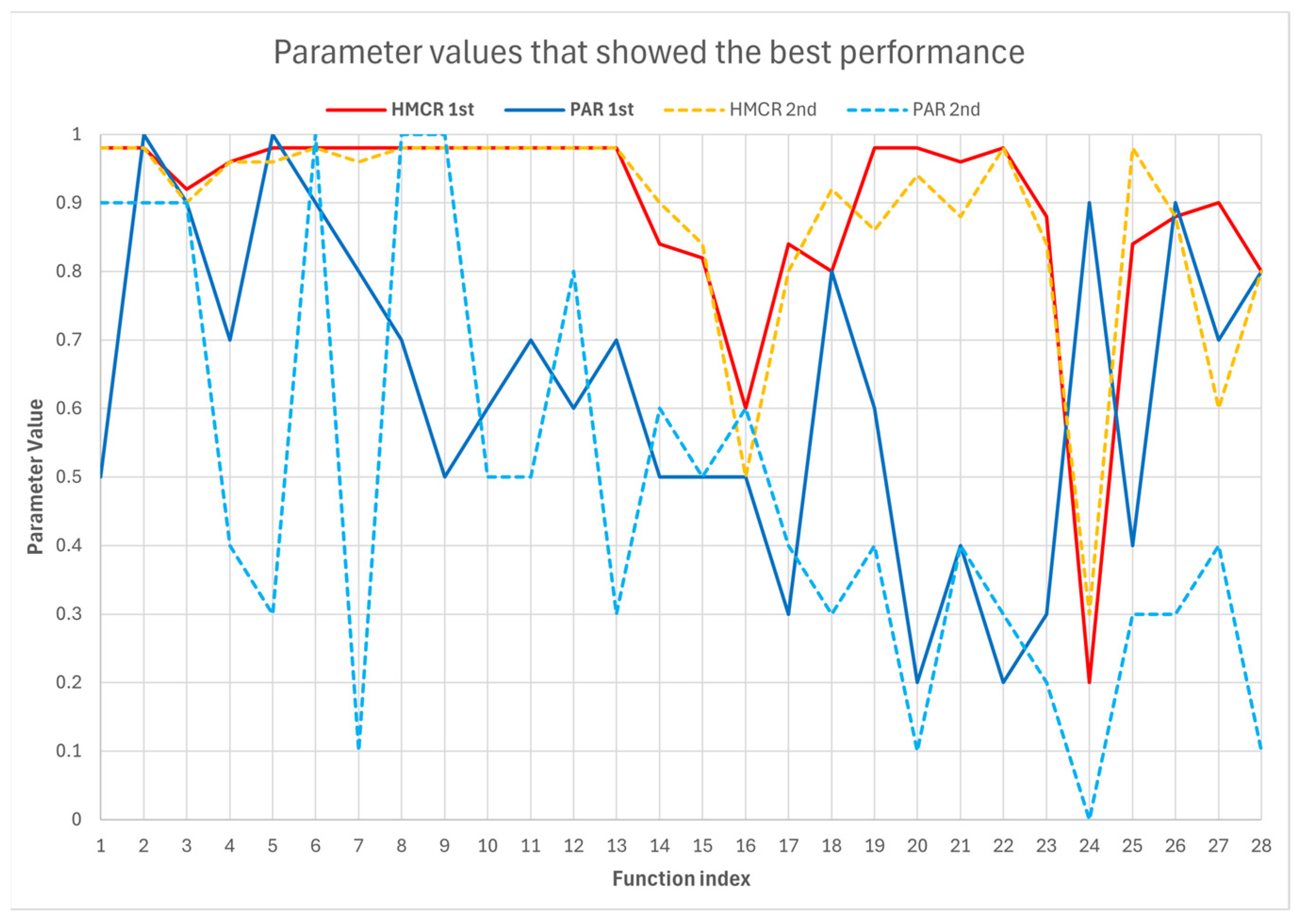
Figure 35 presents the HMCR and PAR values yielding the best and second-best performance across 28 benchmark functions. The horizontal axis denotes the benchmark function indices, while the vertical axis represents the corresponding HMCR and PAR parameter values. The solid line connects the values that achieved the best performance for each benchmark function, whereas the dashed line connects those associated with the second-best performance.

While the general trends provide a broad overview, the topographical characteristics of a specific problem play a crucial role in determining the hyper-parameter values (especially for PAR value).

• Group 1: Unimodal Functions (F1–F7)

For this group of functions, which possess only a single global optimum, the core challenge for the algorithm is the speed and precision of convergence to that optimum. As illustrated by the heatmap for F1 in Figure 7, all functions in this group exhibited the best performance (dark green) at high HMCR values (0.9–0.99). Also, although PAR did not show a clear trend in the heatmap, Figure 35 shows that the top-performing PAR values for F1–F7 are consistently above 0.5, and in most cases exceed 0.7, indicating that for unimodal functions, a PAR setting of no less than 0.5 is generally preferable. This can be interpreted as follows: since the solution space contains no ‘traps’ (local optima), exploration would only lead to unnecessary wandering. Instead, a strong exploitation-dominant strategy, which continuously references good solutions via a high HMCR, proves to be the most efficient approach.

• Group 2: Multimodal Functions (F8–F23)

Group 2 can be further subdivided. First, F8–F13 have a vast, 30-dimensional search space, whereas F14–F23 have fewer dimensions, ranging from 2 to 6. However, the functions in F8–F13 are symmetrical and have a relatively simple structure, while those in F14–F23 are highly complex and feature deceptive landscapes with intentionally placed, difficult traps (local optima).

The results for F8–F13 were largely similar to those for the unimodal functions (F1–F7). The influence of PAR appeared minimal, and consistently superior performance was demonstrated with high HMCR values (≥0.9).

In contrast, for F14–F23, the trends were less consistent, and the green areas in the heatmaps were distributed over a broader range of HMCR values. For instance, the results for F16 in Figure 22 show the best performance at HMCR = 0.6. Similarly, for F17 in Figure 23, while not as pronounced as in F16, numerous cases of good performance were observed at HMCR values of 0.6 or 0.7. This implies that for challenging functions like those in F14–F23, it is often necessary to make significant leaps to escape local optima through random generation, highlighting the greater importance of the exploration-exploitation balance compared to the functions in F1–F13.

Furthermore, whereas the influence of PAR was previously almost invisible, the second set of heatmaps in Figure 22, Figure 23 and Figure 24 revealed that a PAR of 0.3–0.6 yielded good performance, and Figure 25, Figure 26, Figure 27, Figure 28 and Figure 29 showed good performance with a PAR of 0.1–0.3. This can be understood as follows: when viewing HMCR over a wide range (0–1), its dominant influence masks the effect of PAR. However, when the focus is narrowed to a small range like HMCR = 0.8–1.0, the differences in HMCR become less significant, thereby revealing the previously hidden influence of PAR. This demonstrates that while the dominant impact of HMCR in the first heatmaps may obscure the effect of PAR, the second heatmaps reveal that PAR was indeed exerting a subtle influence.

According to Figure 35, which only examines the peak performance points, most F18–F23 models also performed best at HMCRs above 0.9, although some, such as F15–18, performed best at 0.6 or 0.8.

Additionally, F14, 17, and F20–24 also performed best at PAR values lower than 0.5

• Group 3: Real-World Design Optimization Problems (F24–F28)

In Group 3, the variations observed in the challenging problem set of F14–F23 became even more pronounced. For problems 1, 3, and 4, better performance was achieved at lower HMCR values, such as 0.3. Problem 2 showed results that appeared to lack a clear trend, while for problem 5, good results were mostly obtained when HMCR was 0.8.

Looking at the best performance points in Figure 35, the results indicate that high HMCRs between 0.8 and 0.9 perform well, but only F24 shows the best performance at a low HMCR of 0.2.

The group-wise analysis is summarized in

Table 2. Summary of Parameter Influence across Function Groups.

Group	Problem Feature	HMCR Trend	PAR Trend
Unimodal (F1–F7)	Single global optimum	performs best at 0.9–0.99	mostly ≥0.7, with a minimum of 0.5
Symmetric Multimodal (F8–F13)	Large (30) dimensions, Simple symmetric	Similar to unimodal, best at 0.9–0.99	performs best at 0.5–0.7
Complex Multimodal (F14–F23)	Small (2–6) dimensions, tricky local optimum	Best performance spread wider 0.6–0.9	Except for a few cases, the values are generally low (≤0.5)
Real-world Design problems (F24–F28)	Constrained, Highly complex	High values (0.8–0.9) were mostly superior; however, in some cases, very low values (0.2–0.3) turned out to be better.	Mixed trends

.

5. Conclusions and Future Works

This study empirically analyzed the influence of the HS algorithm’s core parameters, HMCR and PAR, on its performance. Extensive experiments were conducted on 23 benchmark functions with diverse characteristics and 5 real-world optimization problems, with the results presented visually through rank-based heatmaps.

The sensitivity analysis revealed that the performance of the HS algorithm is substantially more sensitive to the HMCR value than to PAR. Specifically, it was experimentally established that setting a high HMCR value (≥0.9) is advantageous for securing overall algorithmic stability and performance. It is crucial to note, however, that the extreme case of setting HMCR to 1.0 could lead to severe performance degradation. This is attributed to the complete elimination of random generation, which significantly increases the likelihood of the algorithm becoming trapped in local optima.

The role of PAR manifested differently depending on the topographical complexity of the problem. For problems with a single optimum or relatively simple multiple optima (F1–F13), a high HMCR value 0.9–0.99 had a dominant influence, while a low to medium PAR 0.1–0.3 showed efficient performance. This signifies the importance of an exploitation strategy that leverages existing superior solutions when the solution space complexity is low. Conversely, for complex functions containing numerous local optima (F14–F23) and some real-world problems (F24–F28), a relatively higher PAR value 0.3–0.5 proved more effective for global optimum search. This result indicates that for high-difficulty problems, an adequate exploration capability—that is, securing solution diversity through pitch adjusting—is effective for escaping local optima.

Through these experimental results, this study reinforces the empirical foundation for setting the HMCR and PAR parameters in the HS algorithm. By providing practical guidelines for parameter tuning based on problem characteristics, this research contributes to enhancing the algorithm’s efficiency and applicability.

Future research is expected to devise methods to further enhance the robustness and convergence speed of the HS algorithm based on the insights from this preliminary but fundamental study. Additionally, future work will investigate dynamic parameter setting methodologies that have been studied in various other metaheuristic algorithms and adapt them for the HS algorithm. for example, in the early iterations where global exploration is expected to be more important, the HMCR could be maintained at a relatively low level, and as the iterations proceed, its value may be gradually increased up to around 0.9—while ensuring that it does not reach 1.0—to enhance exploitation in the later stages.